Path Planning of Intelligent Mobile Robots with an Improved RRT Algorithm

Abstract

The Rapidly Exploring Random Tree algorithm, renowned for its randomness, asymptotic properties, and local planning capabilities, is extensively employed in autonomous driving for path planning. Addressing issues such as pronounced randomness, low search efficiency, inefficient utilization of effective points, suboptimal path smoothness, and potential deviations from the optimal path in the RRT algorithm based on random sampling, we proposed an optimization algorithm that integrates Kalman filtering to eliminate redundant points along the path. Initially, this algorithm addresses the issue of inverse growth in the RRT algorithm’s search tree by implementing a variable steering angle strategy, thereby minimizing oscillations and unnecessary pose adjustments. Secondly, by merging collision detection with Kalman filtering, and by comparing the step sizes between newly generated child nodes and random tree nodes towards the root node, we filtered redundant points from the path, thereby reducing the count of effective points and optimizing the path. Lastly, we utilized a second-order Bezier curve to smoothen the path, eliminating sharp corners and discontinuities, ultimately yielding the optimal path. Across diverse map environments and two distinct dimensional scenarios, we conducted multiple sets of simulation experiments to validate the algorithm’s feasibility. The experimental outcomes demonstrate notable improvements in parameters like average path length, average planning time, average count of effective points, and average sampling points, highlighting the enhanced accuracy and efficiency of the improved algorithm in path planning.

1. Introduction

In recent years, the development of mobile intelligent robots has been flourishing and has been widely applied in various fields to complete different types of tasks [1]. Among them, the rapid development of robots cannot be separated from the support of autonomous driving, which is achieved on the basis of path (trajectory) planning. How to make path planning more accurate, reasonable, and optimal core technology has always been a prominent research topic on autonomous and controllable mobile intelligent robots [2]. At present, path planning is one of the autonomous driving decision-making modules, which can be generally divided into five categories: graph search-based, sampling-based, curve interpolation, numerical optimization, and deep learning algorithms. The trajectory planning algorithms based on graph search mainly include Dijkstra’s algorithm [3] and A * algorithm [4,5,6]. Among them, A * algorithm, as a heuristic algorithm, combines priority search and Dijkstra’s algorithm to better balance the relationship between search and utilization. It has fast search speed and ideal search results, but both algorithms will encounter local optimal solutions in the process of path planning, resulting in low search efficiency and greatly affecting planning efficiency. The path planning algorithm based on curve interpolation [7] includes two methods: curve element combination method and interpolation fitting method. Its implementation is simple and the calculation speed is fast, making it suitable for smooth path generation. However, it cannot handle obstacles in complex environments, resulting in poor planning accuracy. The planning algorithm based on numerical optimization [8] uses numerical optimization methods to be solved online, which can find the optimal path and consider complex constraints, but it has high computational complexity and requires a lot of computation time and resources. With the development of data science and big data technology, deep learning algorithms [9,10,11] are gradually being applied to autonomous driving and mainly divided into two categories: simulation learning and reinforcement learning. Simulation learning trains a dataset after collecting driving data to form a neural network, realizing the mapping between environmental states and driving. Reinforcement learning drives the reinforcement learning agent to explore the strategy space and obtain the optimal or suboptimal trajectory that can complete the driving task in the process of interacting with the environment by setting a reward function [12,13,14]. However, due to the certain gap between the virtual environment simulated by computers and the real environment, namely uncertain variable factors such as light, friction, and slippage, interacting with the environment faces huge challenges. If real robots are directly used for data exchange, the collection price is high. Therefore, it cannot be widely applied.

The Rapidly Exploring Random Tree algorithm, as a sampling-based path planning algorithm, operates by expanding and growing new branches within an unknown environment, akin to a tree. It continuously searches and determines whether collisions occur in the surrounding environment while planning the route, ultimately reaching the target range to complete the path planning. Owing to its high search efficiency and strong probabilistic completeness, the RRT algorithm is also applicable to multi-dimensional environments and not just two-dimensional ones, frequently serving as one of the preferred algorithms for path planning in fields like robotic arms and autonomous driving [15,16].

In response to the aforementioned issues, numerous scholars have proposed improvement measures for traditional RRT algorithms. Liu Chong et al. [17] introduced a sampling strategy based on dynamic probability and a random tree expansion strategy with variable step sizes. This approach reduces the number of sampling points, preventing the robot from getting stuck in local minima during path planning. Luo Yi et al. [18] proposed a dynamic path planning algorithm for unmanned aerial vehicles that integrates improved Bi-RRT and DWA. By setting heuristic functions, dynamic step sizes, and safety distances, the Bi-RRT algorithm is enhanced, enabling precise tracking of the global optimal path planning and efficient local obstacle avoidance. Lixin Zhang et al. [19] introduced an improved RRT algorithm with a restricted sampling area (RSA-RRT). For narrow areas, it proposes a fixed angle sampling strategy, achieving shorter paths in less time and effectively balancing path quality and planning speed.

Based on the improvements to the RRT algorithm and existing research results, this article first proposes a variable steering angle strategy on the traditional RRT algorithm to prevent the random search tree from experiencing reverse growth, thereby improving search efficiency. Secondly, Kalman filtering is incorporated into the strategy for redundant point removal, which deletes redundant points along the path while reducing the number of effective points on the path to some extent, thereby forming a new path, improving search efficiency, and reducing path length. Finally, second-order Bezier curves are used to smooth the waypoints along the path.

2. Improved RRT Path Planning Algorithm

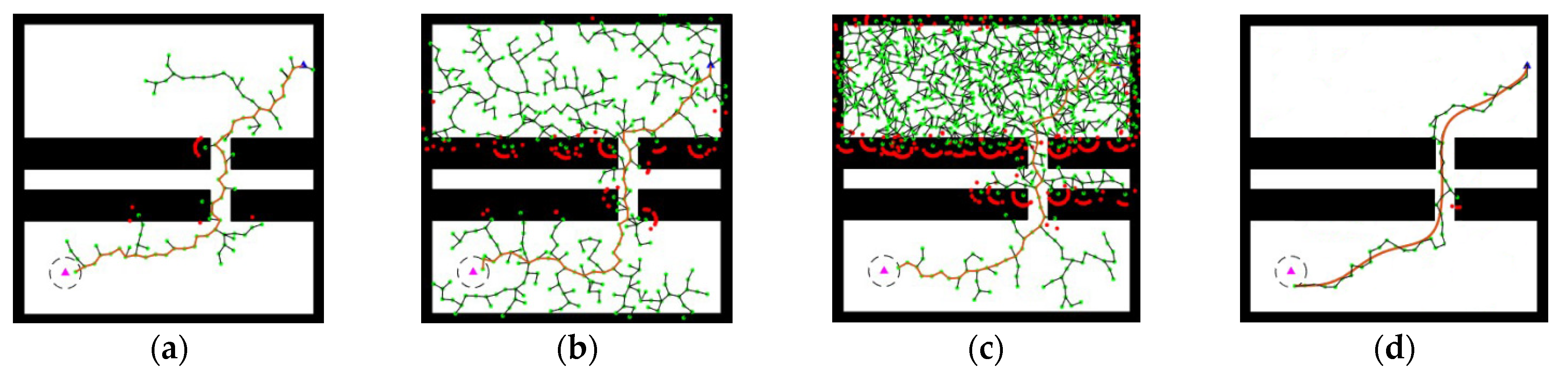
2.1. The Fundamentals of RRT Algorithm

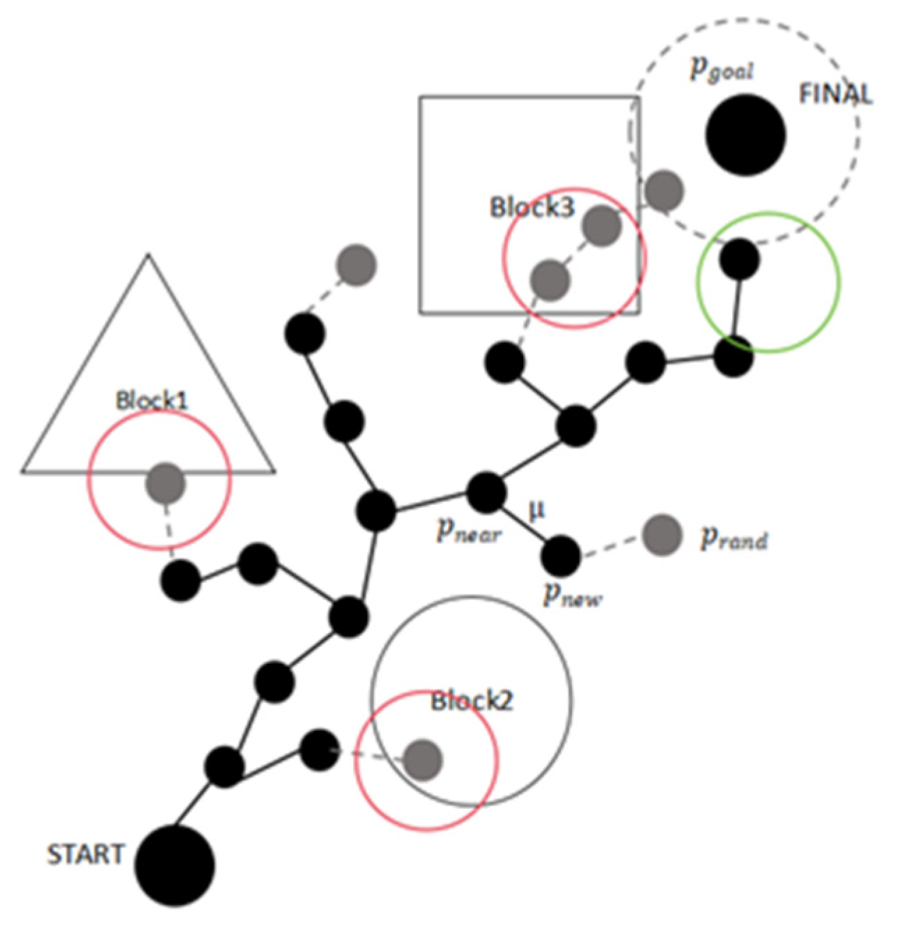
In the field of autonomous driving, the Rapidly Exploring Random Tree (RRT) algorithm based on sampling planning is widely used for path planning. The idea is to treat the initial node as the root node and, through a finite number of random samples, increase the leaf nodes to generate a randomly expanding tree. When the leaf nodes of the random tree reach the target point or target area, an optimal or suboptimal collision-free path can be found from the initial node to the target point within the tree. As shown in Figure 1, the green area represents the final path points, the red area indicates obstacle collision detection, the gray dashed area is the reachable region, and $\mu$ represents the step size.

The RRT algorithm has strong search capabilities, and as long as there is a feasible path in the environment, the RRT algorithm can find a feasible path. However, the traditional RRT algorithm, while exhibiting strong randomness, also introduces several drawbacks. For example, the direction of growth of the random tree during expansion is quite random, leading to low search efficiency, slow convergence speed, and issues such as lack of stability and deviation from the optimal solution in dynamic environments.

To optimize the traditional RRT algorithm, this paper proposed a variable steering angle strategy that integrates Kalman filtering with the RRT algorithm and incorporates collision detection. This approach filters redundant particles through Kalman filtering, thereby enhancing search efficiency and accuracy.

2.2. Variable Steering Angle Strategy

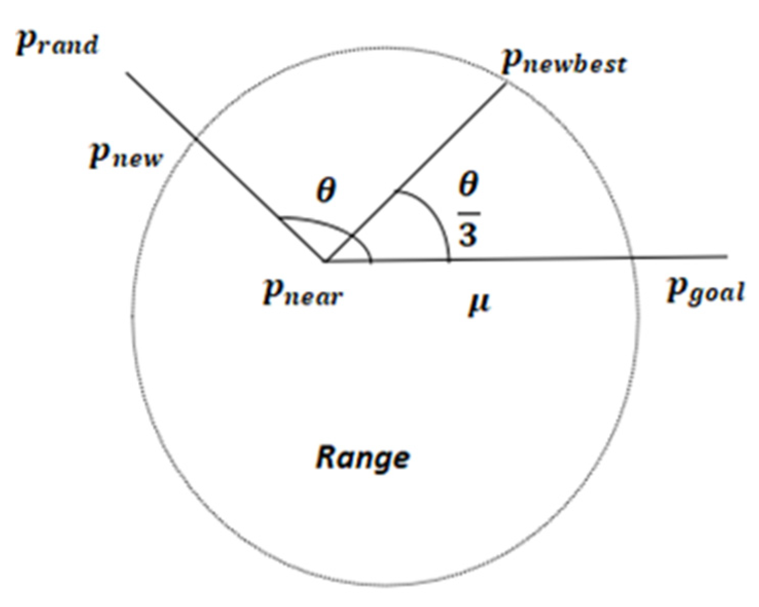
The principle behind the variable steering angle strategy is to prevent the search tree from growing in a reverse direction. This strategy is based on the concept of RRT node extension. When the sampling area narrows down to a specific range, the growth of new branches, without constraints on the steering angle, may deviate from the target point, creating unnecessary branches and generating a large number of redundant search nodes. As a result, search efficiency and accuracy are reduced. However, blindly pursuing high directionality can also lead to local oscillations, which in turn reduces search efficiency. This article introduces a variable steering angle strategy, the principles of which are illustrated in Figure 2.

In the Range region, after the random tree child node $p_{rand}$ finds the closest point $p_{near}$ in the tree, a new child node $p_{new}$ is generated according to the preset step size $\mathsf{\mu }$. If the distance between two points is less than $\mathsf{\mu }$, then $p_{rand}$ is taken as the new search node; if the distance between two points is greater than $\mathsf{\mu }$, then $p_{new}$ passes the collision detection, and at this point, the angle $\mathsf{\theta }$ is greater than 90° between the connecting line of $p_{new}$, $p_{near}$ and the connecting line between $p_{near}$, $p_{goal}$, then it means that the tree branching sub-node There is a reverse growth situation where, in order to solve this problem, the steering angle $\mathsf{\theta }$ is changed to one-third of the original to generate a new child node, $p_{newbest}$, as a child node of this search tree. The formula for updating the steering angle is shown in Equation (1).

$$\mathsf{\theta }=\left\{\begin{array}{c}\theta , \theta ϵ\left[0,{\displaystyle \frac{\pi }{2}}\right]\\ {\displaystyle \frac{\theta }{3}}, \theta ϵ\left({\displaystyle \frac{\pi }{2}}\right., \left.\pi \right]\end{array}\right.$$

(1)

In the above equation, when $\theta ϵ\left[0, {\displaystyle \frac{\pi }{2}}\right]$, no steering angle processing is required; otherwise, the steering angle is updated to one-third of the original. Defining $\mathsf{\tau }$ as the updated step size, q as the sum of the normalized vectors of the new child node’s outward extension, and $p_{newbest}$ as the child node after the variable steering angle strategy, the new node generation equations are as follows:

$$\mathsf{\tau }=\min \left(\left|{\mathrm{p}}_{\mathrm{rand}}-{\mathrm{p}}_{\mathrm{near}}\right|, \mathsf{\mu }\right)$$

(2)

$$q={\displaystyle \frac{{\mathrm{p}}_{\mathrm{goal}}-{\mathrm{p}}_{\mathrm{near}}}{{\parallel {\mathrm{p}}_{\mathrm{goal}}-{\mathrm{p}}_{\mathrm{near}}\parallel }_2}}+{\displaystyle \frac{{\mathrm{p}}_{\mathrm{rand}}-{\mathrm{p}}_{\mathrm{near}}}{{\Vert {\mathrm{p}}_{\mathrm{rand}}-{\mathrm{p}}_{\mathrm{near}}\Vert }_2}}$$

(3)

$$p_{newbest}=\left\{\begin{array}{c}{p}_{near}+\tau \times {\displaystyle \frac{x_{rand}-x_{near}}{{\Vert x_{rand}-x_{near}\Vert }_2}} , 0\le \theta \le {\displaystyle \frac{\pi }{2}}\\ p_{near}+\tau \times {\displaystyle \frac{q}{{\Vert q\Vert }_2}} , {\displaystyle \frac{\pi }{2}}\le \theta \le \pi \end{array}\right.$$

(4)

2.3. Collision Detection and Kalman Filter Redundancy Point Elimination

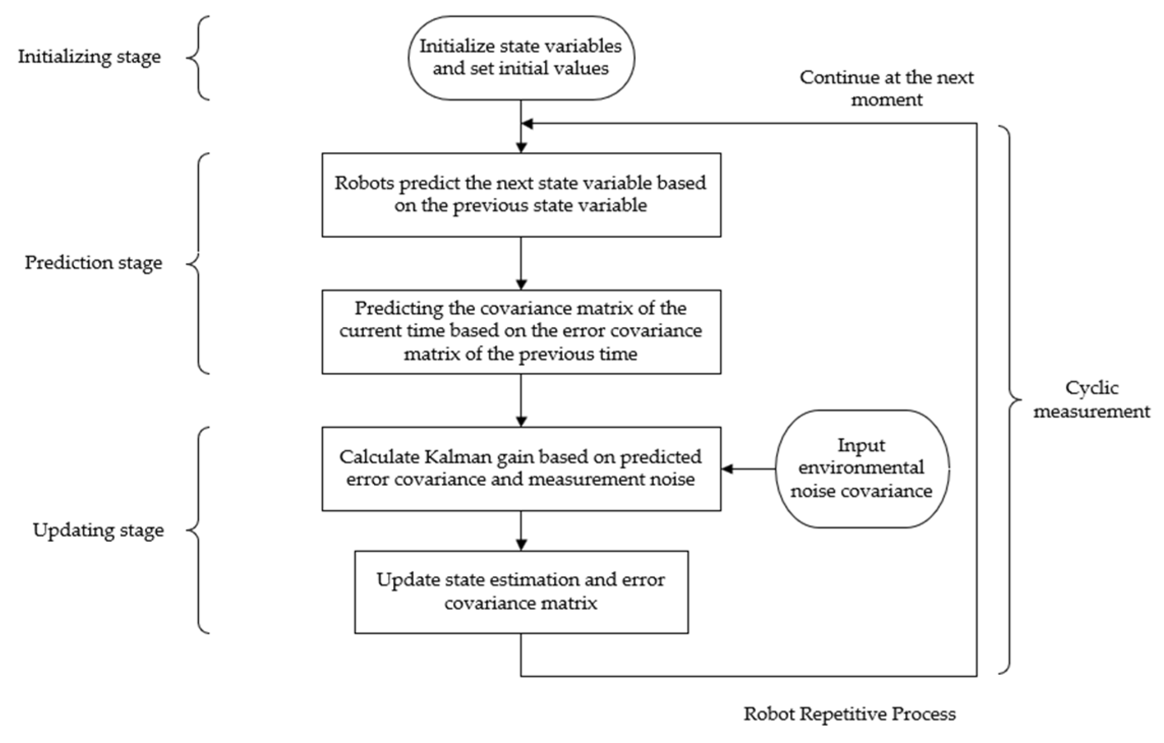
Although the algorithm has been improved by the variable steering angle strategy proposed in this paper, the path searched for the first time may still contain more redundant points, which produces oscillations and unnecessary bit position adjustments during path planning. In this paper, based on the Kalman filtering algorithm, the current node passes through the collision detection, and then the step lengths between the node $p_{rand}$ and the node $p_{new}$ are compared, in which nodes with larger step lengths are filtered out through the Kalman gain until nodes with larger step lengths are no longer passed through this point for searching. There is no more searching through this point at this stage, and instead the prediction state of the next steering is adjusted.

Kalman Filtering is an autoregressive filtering method based on the minimum variance criterion, and its core principle originates from Bayesian filtering theory. The mathematical expressions are shown in Equations (5) and (6).

$$x_t=A{x}_{t-1}+B{i}_t$$

(5)

$$y_t=H{x}_t+o_t$$

(6)

In the above equation, $x_t$ is the state of the environment in which the robot is located at time t, A is the state transition matrix, B is the input control matrix, y_t is the observation value of the environment by the robot at time t, $i_t$ is the input noise, and $o_t$ is the observation noise. H is the observation matrix, as shown in Equation (7).

$$H=\left[\begin{array}{cccc}{h}_{11}& h_{12}& \dots & h_{1n}\\ h_{21}& h_{22}& \cdots & h_{2n}\\ ⋮& ⋮& \ddots & ⋮\\ h_{p1}& h_{p2}& \cdots & h_{pn}\end{array}\right]$$

(7)

The observation matrix maps the system state $x_t$ to the observation space and describes how the system state affects the measurements. The dimension of H is $p\times n$, where p is the number of observation variables and n is the number of state variables. The observation matrix H describes which state variables in the state vector $x_t$ contribute to the measurements.

The robot predicts the next state and error covariance based on a known dynamic model and then calculates the Kalman gain based on the predicted error covariance and measurement noise. The Kalman gain formula is shown in Equation (8).

$$K_n={\displaystyle \frac{P_n{H}^T}{H{P}_n{H}^T+R}}$$

(8)

In the above equation, R represents the covariance matrix of the node measurement noise, ${\mathrm{P}}_{\mathrm{n}}$ is the covariance matrix of the nth node a priori estimation, ${\mathrm{H}}^{\mathrm{T}}$ is the transpose of the measurement matrix H, and ${\mathrm{K}}_{\mathrm{n}}$ is the Kalman gain of the nth time. Under the assumption of constant time, the robot’s state is updated based on the measurements, and the target movement point is determined, significantly reducing the computational time complexity of the random tree during the search.

The flowchart of the Kalman filter algorithm is shown in Figure 3.

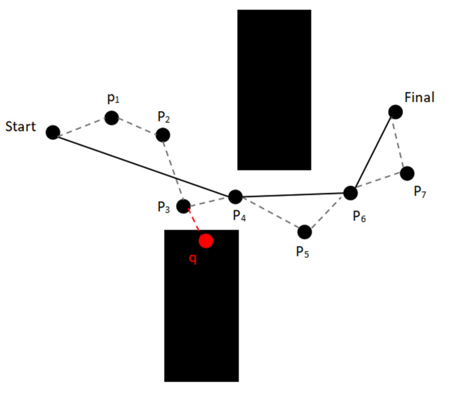
Redundant points in path planning refer to unnecessary nodes between the starting point and the target point. Removing these points can make the path simpler while reducing the number of node observation pose, thereby improving search efficiency. Based on the fundamental principles of the Kalman filter algorithm, this paper estimates the node states through the mapping of the observation matrix H, predicting the future position of the nodes and evaluating the necessity of the nodes. The principle of redundant node elimination based on the Kalman filter is shown in Figure 4.

As shown below, the black node Start is the starting point, Final is the target point, and points $p_1~p_7$ are the path planning points, with a total of seven points. The black solid line is the Kalman filtered path: $\mathrm{Start}\to {\mathrm{p}}_4\to {\mathrm{p}}_6\to \mathrm{Final}$, and the gray dashed line is the initial path, where it can be seen that the number of nodes between the start point and the target point is reduced significantly, which shortens the frequency of nodes adjusting their own position in path planning. q is the collision detection node of node $p_3$, which adjusts its position through collision detection, and combines with the variable steering angle strategy to get the next child node $p_4$.

In the process of path planning, in addition to ensuring the path is optimal, it is also essential to guarantee the smoothness of the path. The higher the smoothness, the higher the controllability. This paper uses Bezier curves for path smoothness optimization. Bezier curves can generate smooth, continuous curves, reducing sharp corners and discontinuities in the path, while also avoiding unnatural movements or acceleration changes. In robot path planning, smooth paths can reduce sudden changes in the robot’s motion, thereby improving the stability and accuracy of movement.

In this paper, a second-order Bezier curve is used to give three control points, $P_1$, $P_2,$ and $P_3$, where $P_1$ and $P_2$ form a first-order Bézier curve while $P_2$ and $P_3$ form a first-order Bézier curve, i.e:

$$\left\{\begin{array}{c}{P}_{1,2}=\left(1-t\right)P_1+t{P}_2\\ P_{2,3}=\left(1-t\right)P_2+t{P}_3\end{array}\right.$$

(9)

On the basis of generating two first-order points through Equation (9), a second-order Bessel point $p_3^2$ is generated through Equation (10).

$$p_3^2=\left(1-t\right)P_{1,2}+t{P}_{2,3}$$

(10)

to obtain a second-order Bezier curve:

$$p_3^2={\left(1-t\right)}^2{P}_1+2t\left(1-t\right)P_2+t^2{P}_3$$

(11)

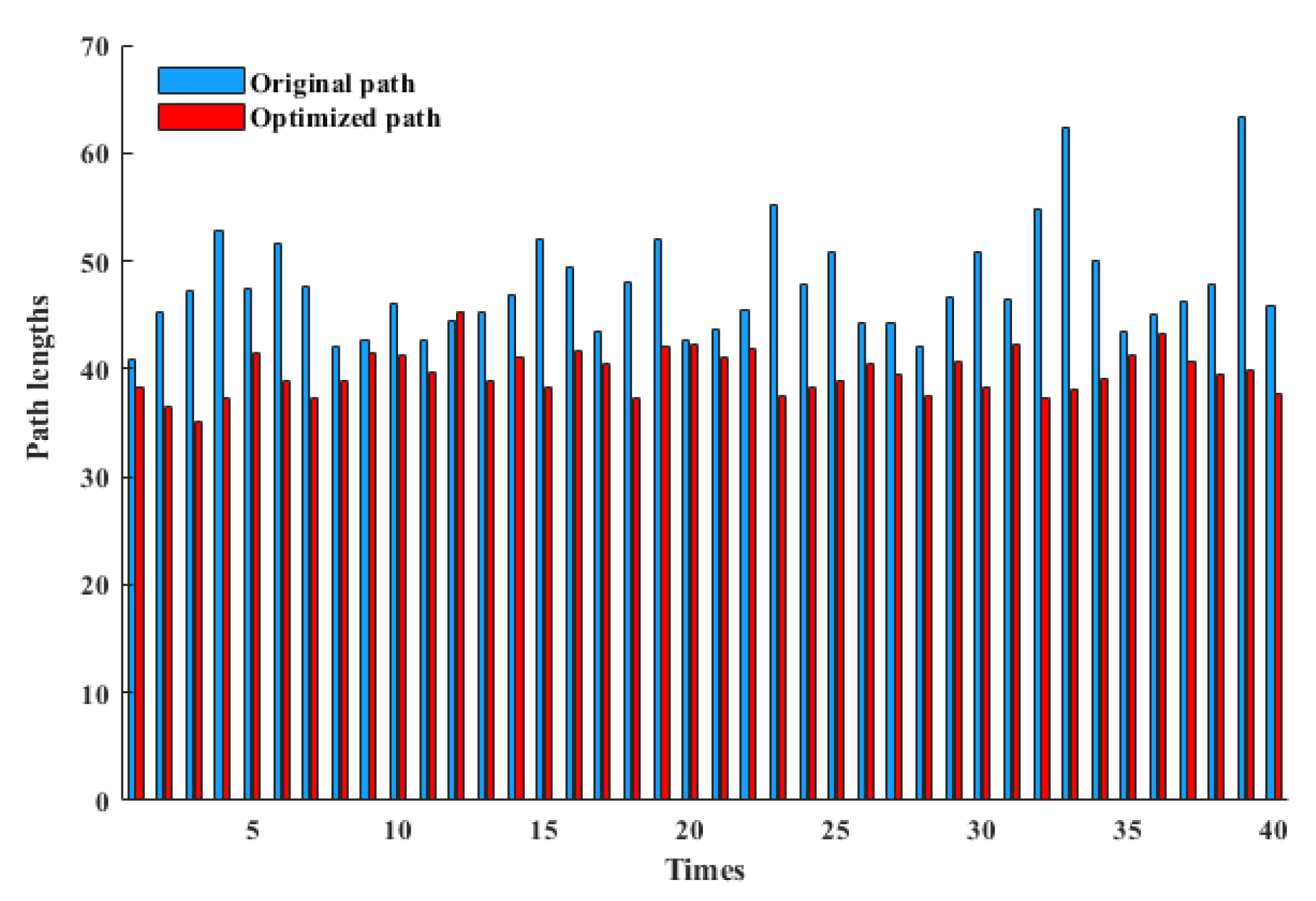
With t taken at equal intervals from 0 to 1, the path of the final curve after second-order Bezier smoothing is shown in Figure 5. In this figure, the time values from (a) to (d) are 0.182 s, 0.479 s, 0.708 s, and 1 s.

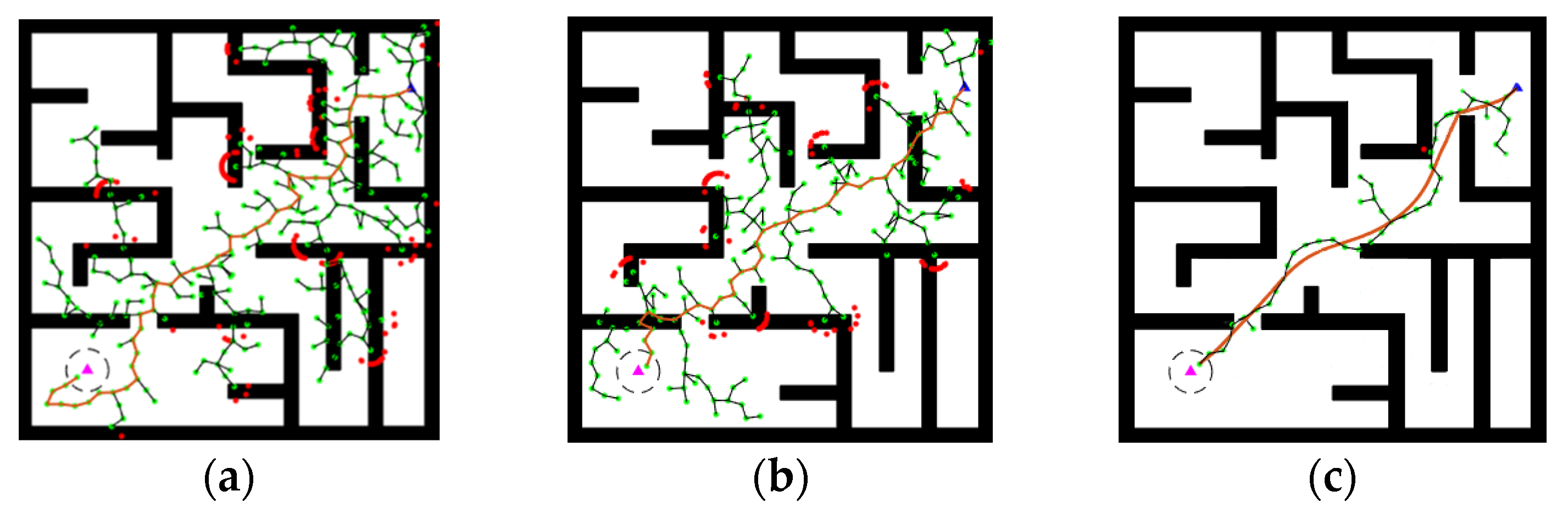
2.4. Improved RRT Algorithm Framework Model

The improved RRT-KF algorithm is built on the traditional RRT algorithm, making it more efficient in searching across various environments by incorporating strategies such as steering angle change, redundant point removal based on Kalman filtering, collision detection, and path smoothing using Bezier curves. Starting from the initial point, the algorithm finds the nearest point and then expands toward a random point. At this stage, the steering angle change strategy adjusts the step size and direction during expansion to avoid the phenomenon of nodes growing in reverse, dynamically adjusting the steering angle to increase the algorithm’s flexibility and prevent the algorithm from stalling. During the node growth process, collision detection is used to ensure that the planned path does not pass through obstacles, and the steering angle change strategy helps accurately and quickly lock onto the forward direction. During path generation, unnecessary points may appear between nodes, affecting the path length and efficiency. Based on traditional redundant point removal, Kalman filtering is used to observe and predict the future target position of nodes, determining whether a node is redundant and removing it accordingly. With the smoothing effect of the second-order Bezier curve, the final node can reach the target point along a smooth path, providing a theoretical foundation for the practical application of this algorithm. The pseudocode of the algorithm is shown in Algorithm 1.

Algorithm 1: Improved RRT-KF Algorithm

1. RRT-KF ($x_{start},x_{goal}$)

$2. tree\leftarrow$[node(start)]

$3. neares{t}_{node}\leftarrow find \left(tree,ran{d}_{node}\right)$// Finding the nearest node

$4. ne{w}_{node}\leftarrow VariableSteering \left(neares{t}_{node},ran{d}_{node}, \tau \right)$// Steering angle change strategy

5. if not collision check ($neares{t}_{node}.pos,ne{w}_{node}.pos$) // Collision detection

6. update Kalman filter ($ne{w}_{node}$)

7. float distance = calculateDistance (nodes[i], nodes[j]) // The distance is measured based on the observation matrix H

8. if (distance  $<threshholdDistance$) delete node (nodes, nodeCount)

9. nodes[i] = nodes[i+1]

10. nodeCount — // Redundant point elimination based on Kalman filter

11. tree.append ($ne{w}_{node}$)

12. if distance ($ne{w}_{node}.pos, x_{goal}$$) <GOAL RADIUS$

13. path$\leftarrow extract path \left(ne{w}_{node}\right)$

14. smoothed path$\leftarrow beziersmoothing \left(path\right)$// Bezier curve path smoothing

15. return SmoothedPath

In the above algorithm, given the starting point is $x_{start}$ and the target point is $x_{goal}$, the algorithm begins by searching for nearby child node $neares{t}_{node}$ from $x_{start}$. Using child node $neares{t}_{node}$ as the parent node, the algorithm compares the angle between nodes $ran{d}_{node}$ and $ne{w}_{node}$ to determine if a collision has occurred through the pose. The Kalman filter state of the node is updated, and the distance of the node is checked to see if it lies within the observation values, thus removing redundant points. Finally, the path is smoothed using a Bezier curve, and the SmoothedPath is returned.

3. Experimental Validation

To verify the path planning capability of the improved RRT-KF algorithm in different environments, five experimental environment maps are constructed in this experiment: an obstacle-free map, a multi-channel map, a single-channel map, a complex environment map, and a 3D environment map. The first four scattered maps represent various 2D complex environments, while the 3D scene can validate the algorithm’s performance in high-dimensional space. The size of the first four two-dimensional maps is uniformly 30 × 30, and the algorithm step size $ste{p}_1=1$; the 3D environment map size is 1000 × 1000 × 1000, and the algorithm step size $ste{p}_2=20$. In order to minimize the influence of chance error on this experiment, 40 groups of repeated experiments are conducted, and the collected average path length, average planning time, average number of collision points, average number of sampling points, and average number of valid points (rounding off) are used as experimental evaluation indicators.

3.1. Flow Chart of the Improved RRT-KF Algorithm

The flow chart of the improved path planning algorithm is shown in Figure 6.

3.2. Simulation Experimental Environment

The specific configuration of hardware and software parameters used in this simulation experiment is shown in

Table 1. Hardware and software parameters.

Title	Name	Parameter Configuration
Software	MATLAB	MATLAB R2024a
Hardware	CPU	12th Gen Intel(R) Core(TM) i7-12650H
	GPU	NVIDlA GeForce RTX 3070
	Mainboard	Intel B660

.

3.3. Multi-Map Environment Path Planning Simulation Experiment

In this section, the proposed improved algorithm is compared with the traditional RRT algorithm, with different control groups set for different maps to verify its effectiveness. In the simulation experiments, the improvement of the proposed algorithm is validated by comparing data such as the percentage change in average path length and average planning time, the average number of collisions, and the efficiency of valid samples. The red curve represents the final path before and after the improvement. The simulation results for the obstacle-free map are shown in Figure 7.

From Figure 7a,b and

Table 2. Comparison of accessibility map simulation data.

Algorithm	Average Path Length	Average Planning Time	Average Number of Collision Points	Average Number of Sampling Points	Average Number of Active Points
RRT	39.159	0.103	2	151	37
Improved algorithm	34.945	0.067	0	85	33

, it can be seen that in the accessible map environment, the traditional RRT algorithm, due to its arbitrariness, causes the nodes to disperse to its surroundings randomly, and collisions may occur even in the accessible environment, which is more random, and it is unable to search for the shortest path between the initial point and the target point more accurately. Compared with the traditional RRT algorithm, the average planning time of the search path is reduced by 34.71%, the average path planning length is reduced by 10.76%, and in the case of almost the same valid points, the average sampling point tree is reduced significantly by 43.71% compared with the RRT algorithm, which improves the search efficiency. The above two sets of experiments show that the improved algorithm is more conducive to more accurate path planning with higher efficiency in an obstacle-free environment.

The simulation results of the multi-channel map are shown in Figure 8.

The channels are first labeled as shown in Figure 9. In the 40 sets of experiments in the multi-channel map, the traditional RRT algorithm accounts for 25.00%, 52.50%, and 17.50% of channel 1, channel 2, and channel 3, respectively, in the process of path planning, while the improved algorithm accounts for 100% of channel 2, where it can be seen that the decision-making planning of the paths becomes more accurate after incorporating Kalman filtering. As shown in Figure 8a–d and

Table 3. Comparison of multi-channel map simulation data.

Algorithm	Average Path Length	Average Planning Time	Average Number of Collision Points	Average Number of Sampling Points	Average Number of Active Points	Whether It Is the Best Path	Channel No.1/2/3
RRT	40.310	0.156	23	177	36	Yes	2
	44.297	0.204	31	192	41	No	1
	45.418	0.317	36	227	44	Yes	3
Improved algorithm	31.818	0.071	2	48	33	No	2

, in the multi-channel map scenario, the optimal average path length planned by the improved algorithm is reduced by 21.07% and the average number of samples is reduced by 72.98% compared with the traditional RRT algorithm; the significant reduction of samples indicates that the randomness of the algorithm is reduced, the redundant points are reduced, the average planning time is reduced by 54.49%, and the number of effective points is reduced by a small margin. The comparison of the above two sets of experiments illustrates the path planning ability of the improved algorithm in multi-channel maps.

The simulation results for the single-channel map are shown in Figure 10.

From Figure 10a–d and

Table 4. Comparison of single-channel map simulation data.

Algorithm	Average Path Length	Average Planning Time	Average Number of Collision Points	Average Number of Sampling Points	Average Number of Active Points
RRT	49.723	0.765	334	738	44
Improved algorithm	43.021	0.319	5	275	39

, it can be seen that in a narrow single-channel environment, the RRT algorithm experiences a large degree of collisions and backward growth, as shown in Figure 10b,c. A particle will undergo repetitive collisions in almost the same orientation, which makes it difficult to accurately find the correct path, and the time complexity becomes high in 40 groups of experiments, with only 3 groups finding the correct path, as shown in Figure 10a. In contrast, the improved algorithm in this paper utilizes the variable steering angle strategy to redefine the direction of travel when the node particles grow against the grain; when multiple collisions occur at a node, the particle is filtered using Kalman filtering to avoid redundancy of collisions and improve efficiency. The optimized algorithm reduces the average path length by 13.50% and the average planning time by 59.31% compared with the traditional algorithm, and nearly half of the average sampling points are due to collisions, the optimized average sampling points are reduced by 62.74%, and the effective point utilization rate is increased by 11.36%. The above two sets of experiments illustrate the path planning ability of the improved algorithm under narrow single channel.

Next, by simulating the path planning in a real environment, constructing a raster map in the 2D plane—with black rectangles indicating obstacles—and comparing the path planning ability of the traditional RRT algorithm with the improved algorithm, the simulation results are shown in Figure 11.

Figure 11a shows that the traditional RRT algorithm can find the path from the starting point to the target point, but the node search is more complex and multiple collisions occur. In addition to this, the traditional RRT algorithm has unreasonable path planning as shown in Figure 11b, where the black rectangle is selected to pass in the map. In contrast, the improved algorithm in this paper obtains smooth path curves with fewer collisions, greatly reducing redundant nodes and faster path search.

As shown in Figure 12, the bar graph of the path length comparison between 40 groups of experiments before and after optimization, it can be seen that the optimized paths are shorter than the original paths, and the optimized algorithm is more stable in path planning, which reflects the robustness of the algorithm, and the optimized average paths are reduced by 16.64% compared with the original average path lengths, which reduces the expansion of the random tree nodes’ searches in the irrelevant regions, thus reducing the time to find the initial path and the initial path lengths. This reduces the search expansion of random tree nodes in irrelevant regions, thus reducing the time to find the initial path and the length of the initial path.

In addition to the above four 2D environments, in order to verify the effectiveness of the improved algorithm in 3D environments, three sets of experiments are set up to compare the path planning parameters of the improved algorithm of this paper with those of the traditional RRT algorithm and the RRT–Greedy algorithm in the same map environments, and the simulation results are shown in Figure 13.

From Figure 13a–c, it can be seen that the traditional RRT algorithm for path planning in 3D environment still generates many redundant sub-nodes due to its randomness, while the RRT-Greedy algorithm reduces the planning time and the number of sampling points to a certain extent. From the data in

Table 5. Comparison of simulation data for 3D map environment.

Algorithm	Average Path Length	Average Planning Time	Average Number of Collision Points	Average Number of Active Points	Efficient
RRT	1703.350	0.469	223	85	38.12%
RRT-Greedy	1622.174	0.273	122	81	66.39%
Improved algorithm	1614.759	0.148	97	80	82.47%

, it can be seen that the improved algorithm in this paper, compared with the traditional RRT algorithm and RRT-Greedy algorithm, has a significant reduction in the average path planning length by 5.20% and 0.46%, respectively; the average path planning time is reduced by 68.44% and 45.79%, respectively; the average number of sampling points is greatly reduced by 56.50% and 20.49%, respectively. While the average effective number of path points is almost the same, the effective rate is increased to show the accuracy of the algorithm’s decision-making in the path planning process, and the above three sets of experiments illustrate the feasibility of this paper’s improved algorithm in the three-dimensional map environment.

4. Testing in Real-World Scenarios

To verify the feasibility and accuracy of the improved RRT-KF algorithm for mobile robot path planning in real-world scenarios, the robot used in this experiment is installed with the Ubuntu 22.04 LTS operating system. The underlying drive system uses four Mecanum wheels, enabling operations such as in-place turning and rotation. The robot is equipped with sensors such as LiDAR and IMU. The center-to-center distance of the chassis is 0.25 m, and the maximum speed is 0.45 m/s. The motion code is written using Linux and C++ programming languages to control the robot’s movement, achieving autonomous control of the robot. Real-time data is transmitted via topics, enabling the validation of the proposed algorithm.

4.1. Experimental Platform

The specific configuration and parameters of the experimental platform are shown in

Table 6. Experimental platform configuration and parameters.

Name	Parameter
Operating system	Linux Ubuntu 22.04 LTS (Jammy)
ROS	ROS2 Humble Hawksbill
Programming language	C++
Control language	Linux language

.

The actual robot used in the experiment is shown in Figure 14.

The mobile intelligent robot used in the experiment is equipped with the Laser-C 16 laser radar, which uses a dense 16 beam laser to achieve 360° 3D high-speed scanning. The detection distance is 200 m high, the measurement accuracy is accurate to 3 cm, and the vertical angle resolution is 2°, providing hardware support for the stability of the improved algorithm in this paper.

4.2. Experiment and Result Analysis

The actual experimental scenario chosen for this algorithm is shown in Figure 15. In this experimental scenario, two types of different obstacles are selected to verify the robot’s ability to adjust its steering angles and generate smooth paths under different conditions. The robot’s path planning time and path planning distance are used as evaluation metrics. The actual measurement shows that the shortest path distance is 3.3 ± 0.2 m. In the experimental scenario of Figure 15, 20 sets of experiments are repeated, and the experimental results are recorded. The data is visualized using MATLAB 2024a, and the results are compared with the actual shortest path to validate the accuracy and feasibility of the algorithm.

The trajectory of the mobile intelligent robot in the experiment is shown in Figure 16.

From Figure 16, it can be seen that Figure 16a,f are the starting and ending points of the robot path planning, while Figure 16b–e show the path planning process of the mobile intelligent robot. In Figure 16b,d, when the robot encounters an obstacle, it turns to the original direction through a collision detection algorithm and turns to the endpoint direction under the constraint of the turning angle range, greatly avoiding turning to the other three directions. At the same time, the robot uses a Kalman filter to filter redundant target detection points, making its planning speed faster. The obtained target path points are smoothed through Bezier curves to obtain the final path, which reduces the number of turns and avoids sharp turns, improving the smoothness and stability of the robot’s motion. Figure 17 and Figure 18 are box plots of robot path planning time and path planning length obtained from 20 sets of experiments, respectively.

From Figure 17 and Figure 18, it can be perceived that the average planning time of the mobile robot remained stable at 17.017 s, while the average path planning length was 3.413 m across 20 experiments. Compared to the known measured path length, the planned path remained stable between 3.310–3.485 m and the planning time remained stable between 16.550–17.425 s. This demonstrates that the improved algorithm offers both high stability and accuracy. During the path planning process, the robot may be influenced by physical factors such as light and temperature. In the future, better results could be achieved through optimization of the hardware components.

5. Discussion

This article optimizes the RRT algorithm based on random sampling for autonomous driving path planning. First, in response to the randomness of the traditional RRT algorithm, a variable steering angle strategy is proposed to reduce the number of search nodes in the random tree. Second, for collision point detection, a collision detection method combined with Kalman filtering is proposed to filter out collision points and eliminate redundant nodes, which reduces the number of valid points on the planned path and makes the path planning more precise. Finally, Bezier curves are used to smooth the path and control its curvature to ensure smoothness. The feasibility of the optimized algorithm is verified through simulations in five different map environments. Based on the results of five sets of simulations, the optimized algorithm reduced the average path length by 13.43% and the planning time by 54.24%. Compared to the RRT algorithm, the accuracy of path planning decisions and the planning time have both been significantly improved. Further validation of the algorithm in real-world scenarios demonstrates its feasibility and accuracy.

Through data comparison, it can be seen that the optimized algorithm in this paper performs better than the traditional RRT algorithm. In the future, the optimization of the algorithm will mainly focus on the following aspects:

(1)

Due to differences between the algorithm in the simulation experiment and real-world scenarios, the robot may not be able to capture the more complex situations of the real world during its movement, which presents certain limitations. The robustness of the algorithm in real-world conditions can be further improved in future work.

(2)

Optimizing robot hardware in real-world scenarios can address the limitations of sensor precision, computational power, and response time, thereby further improving the performance of the algorithm. For example, increasing sensor precision can reduce measurement errors, enabling the algorithm to make more accurate decisions and plan more effective paths in real-world conditions. Additionally, optimizing and enhancing the robot’s processor performance, processing speed, and response time can reduce the time required for path planning. Finally, using more reliable hardware can greatly help the robot mitigate the impact of temperature conditions, sensor conditions, and sensor noise in real-world environments.

(3)

Regarding whether the algorithm can be executed in autonomous driving systems, we will conduct further testing to ensure that the improved algorithm can be correctly executed on real-world roads. Additionally, we will use better hardware to address potential limitations and challenges related to sensor accuracy, environmental factors, and computational power. Finally, we plan to conduct further research on filtering algorithms in the future to optimize the algorithm and enhance its adaptability.

(4)

For the improved algorithm in this paper, we will continue research and explore its application and deployment in fields beyond autonomous driving, such as industrial automation and navigation planning, to enhance the algorithm’s robustness and performance in a wider range of applications.