
An Adaptive Compound Control Strategy of Electric Vehicles for Coordinating Lateral Stability and Energy Efficiency


Abstract
1. Introduction
2. System Overview and Vehicle Model
2.1. System Overview
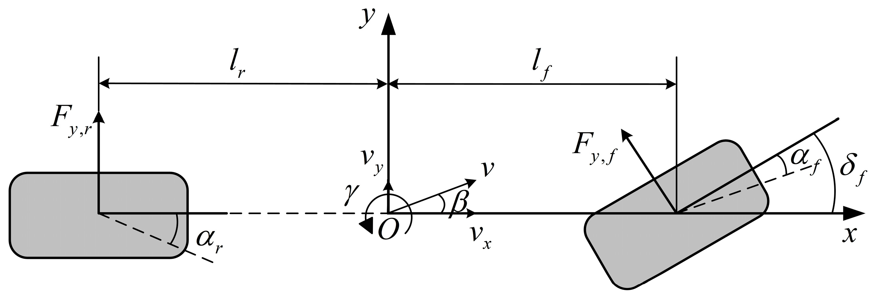
2.2. Vehicle Model
3. Design of an Adaptive Compound Controller for Reference Model
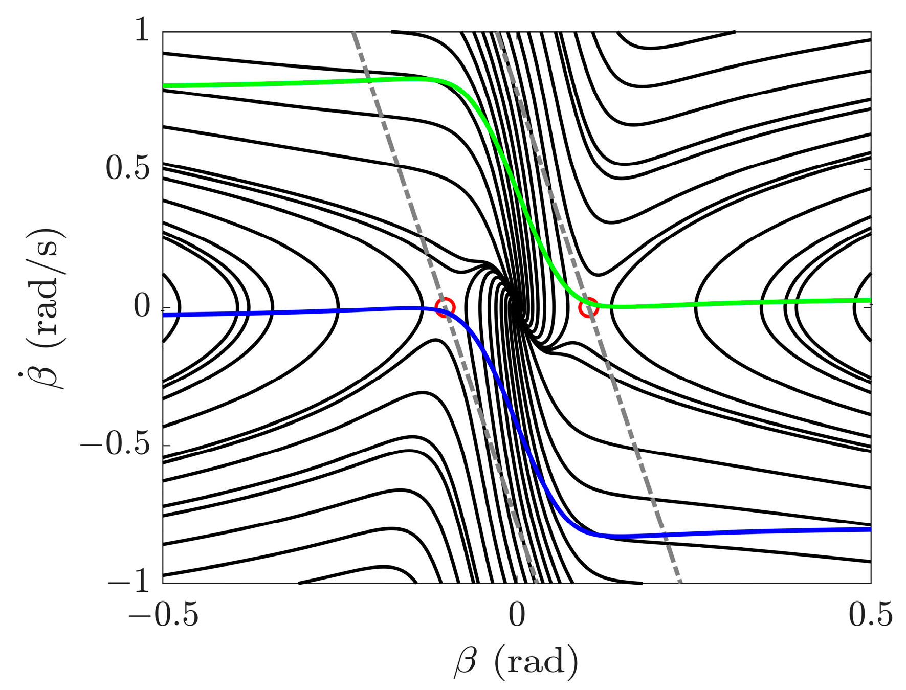
3.1. Dynamics of the Reference Vehicle Model
3.2. Upper-Layer Controller
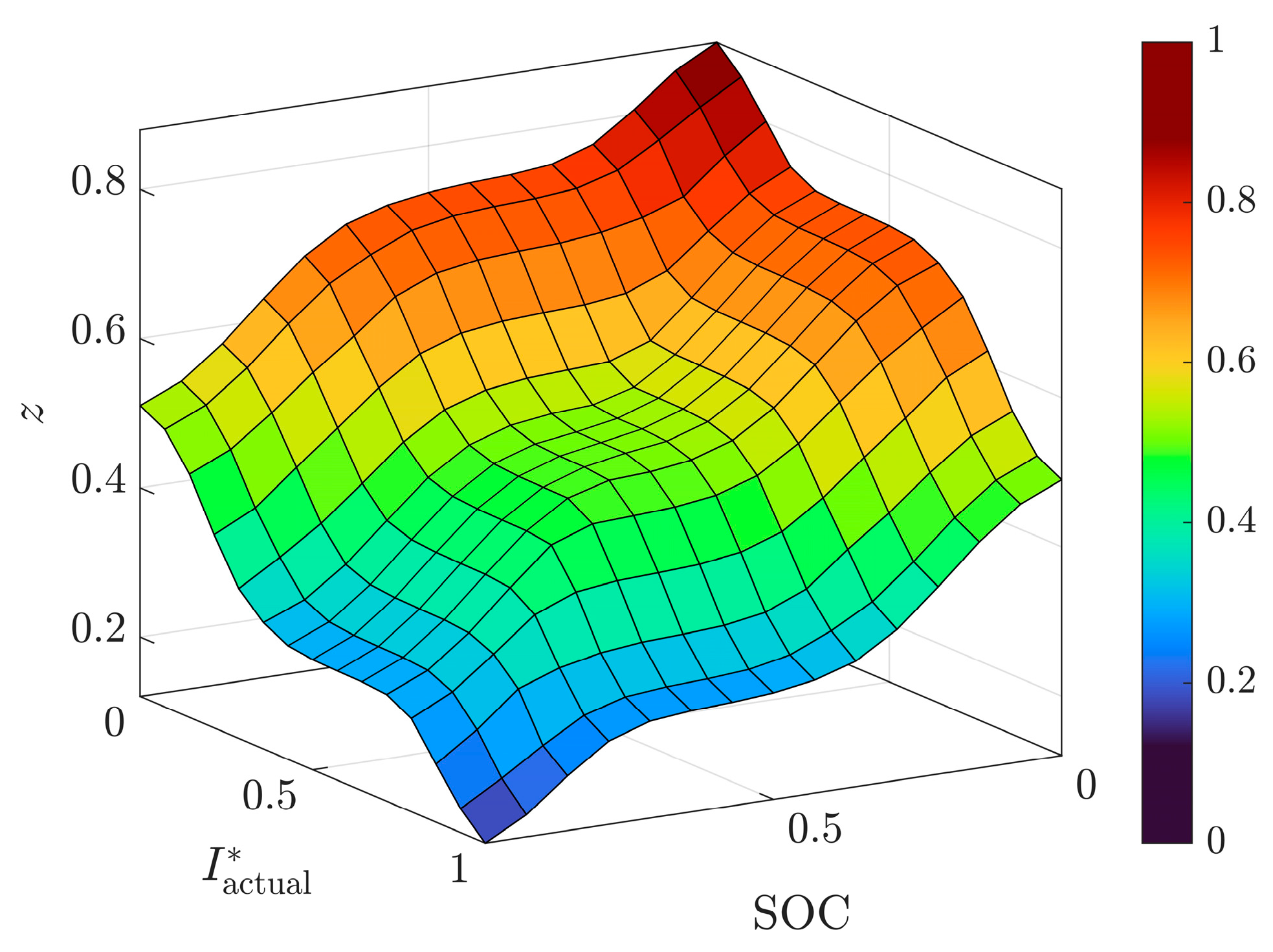
3.3. Adaptive-Layer Controller
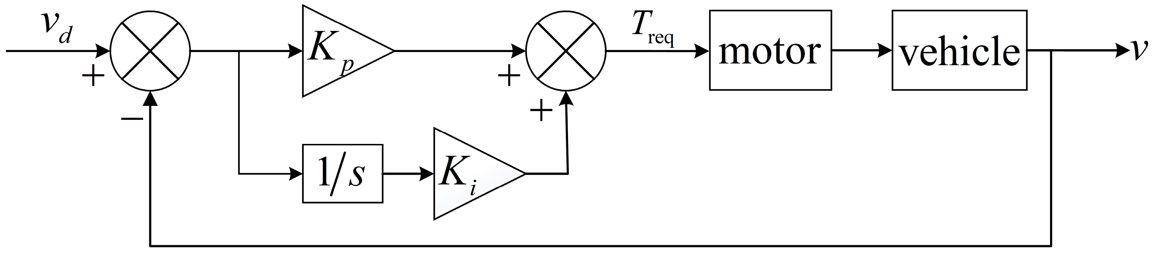
3.4. Lower-Layer Controller
4. Numerical Simulations
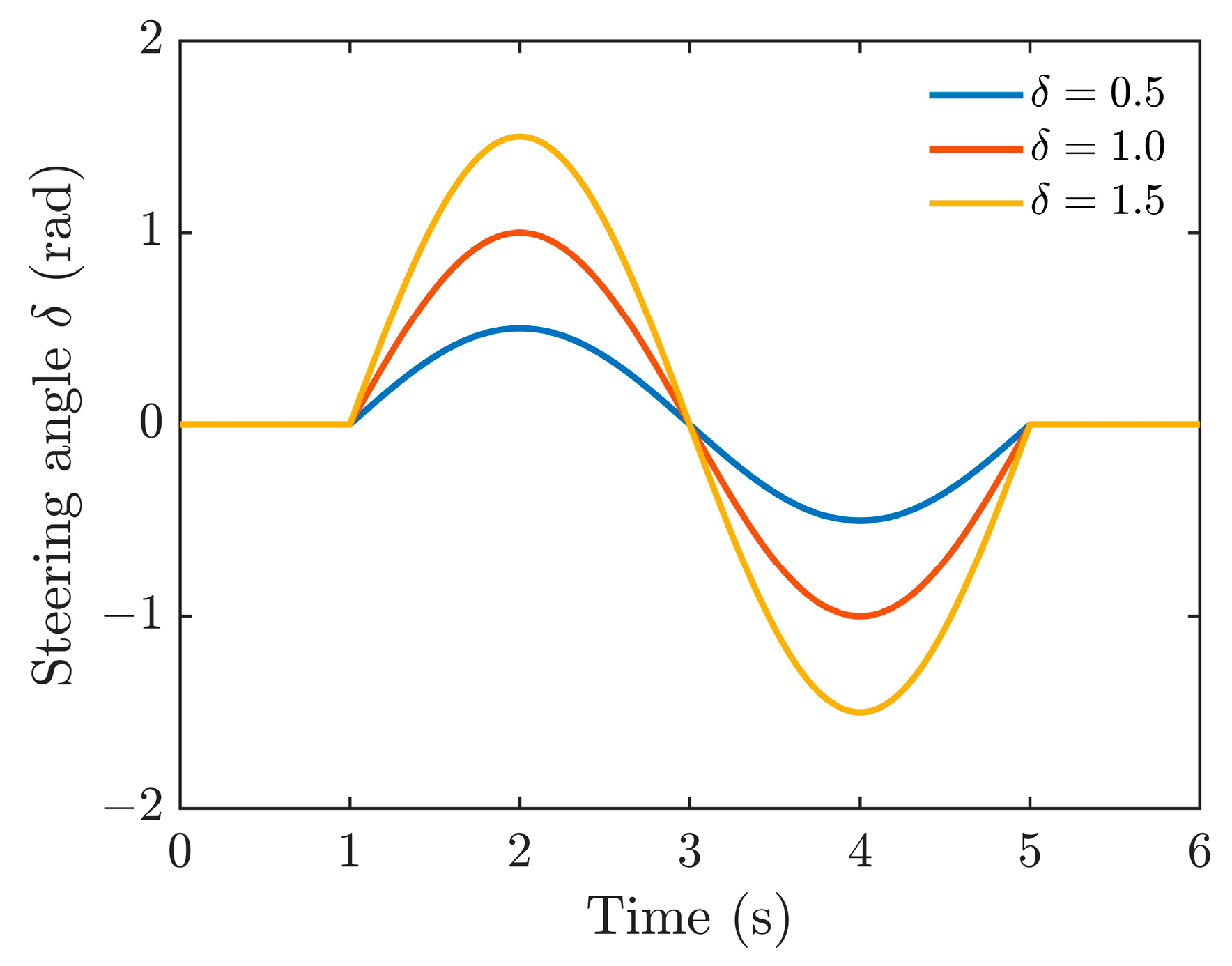
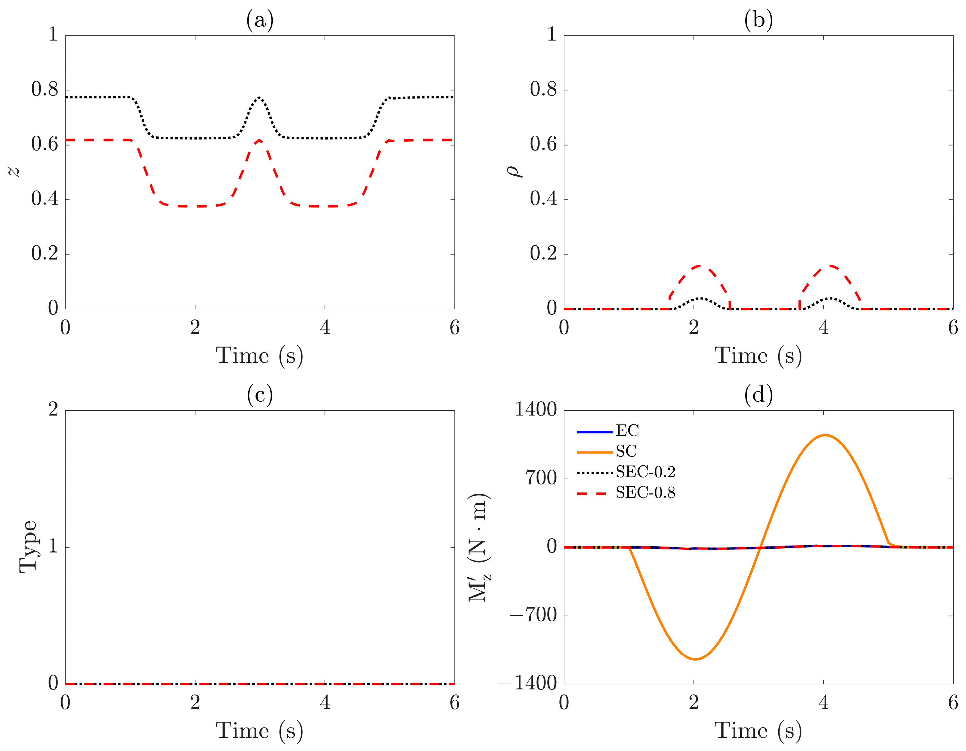
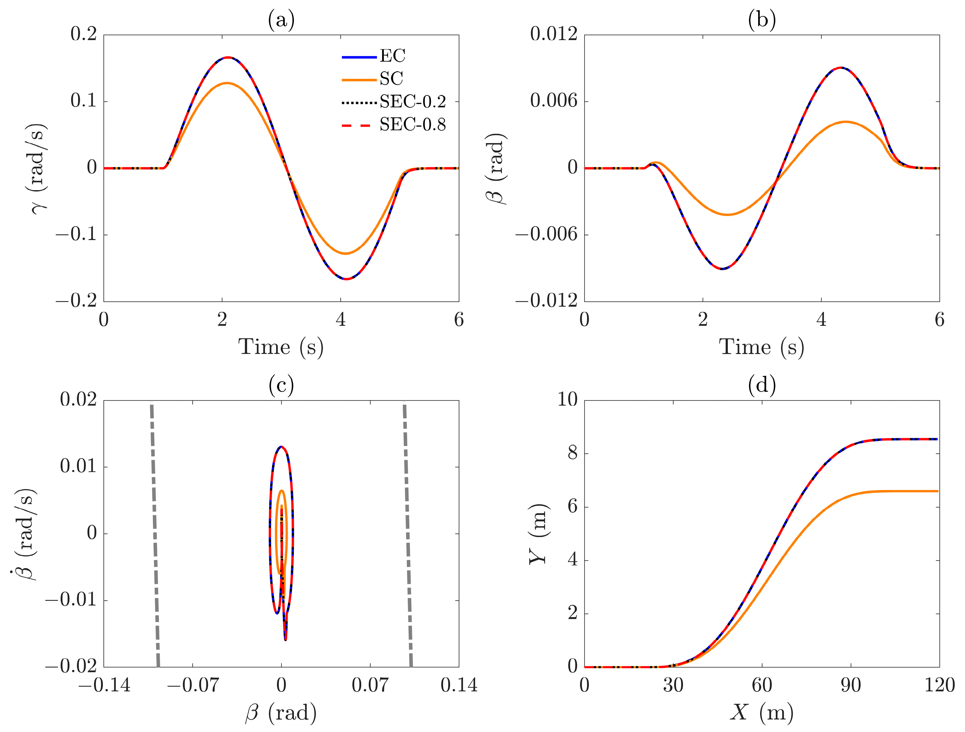
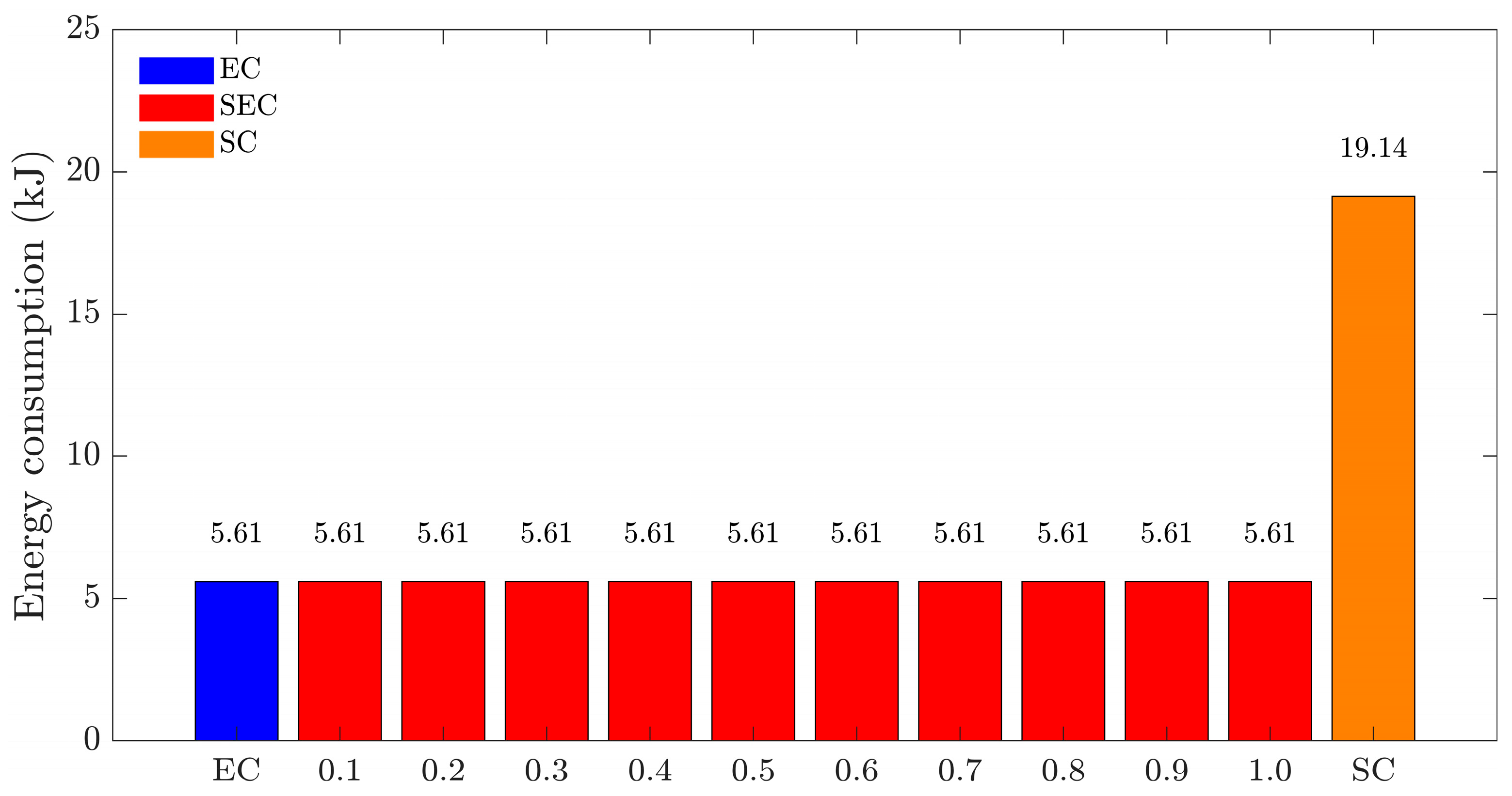
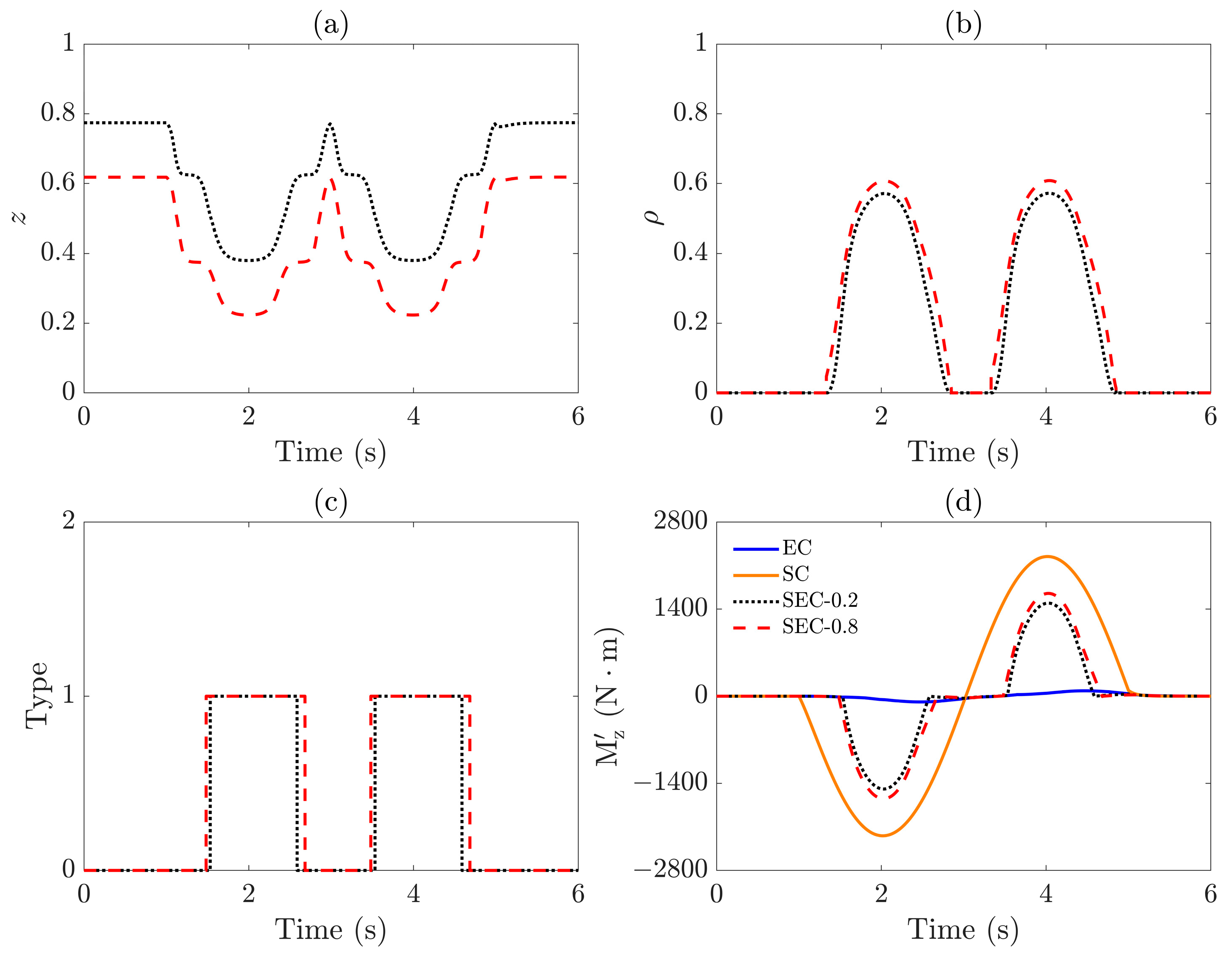
4.1. Case 1:
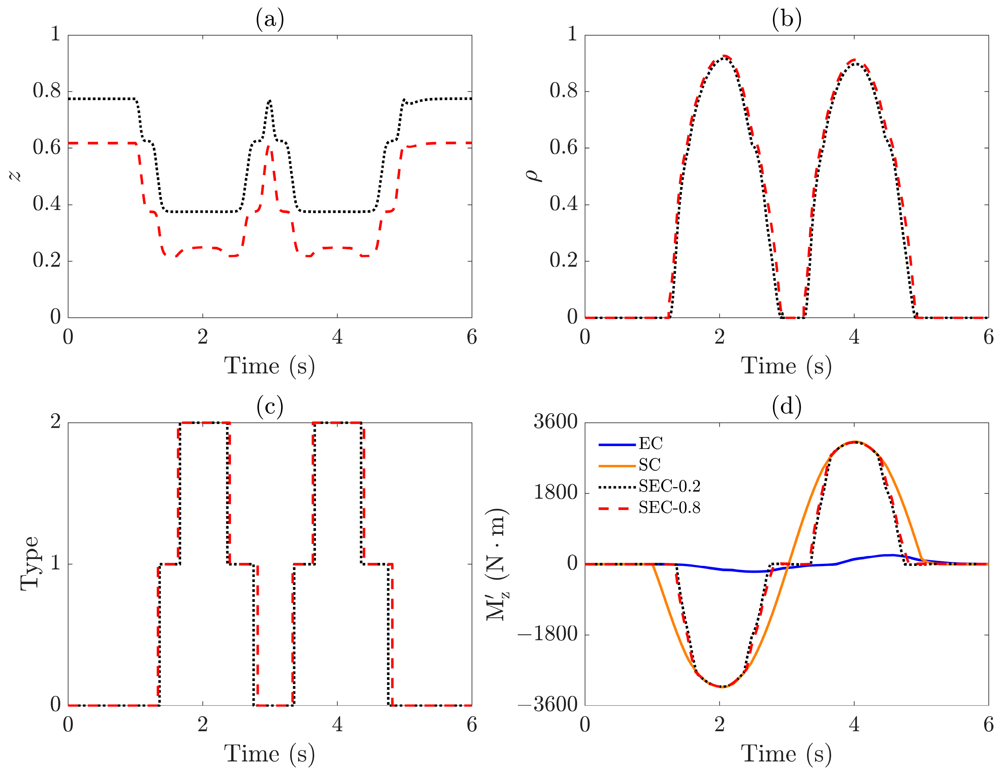
4.2. Case 2:
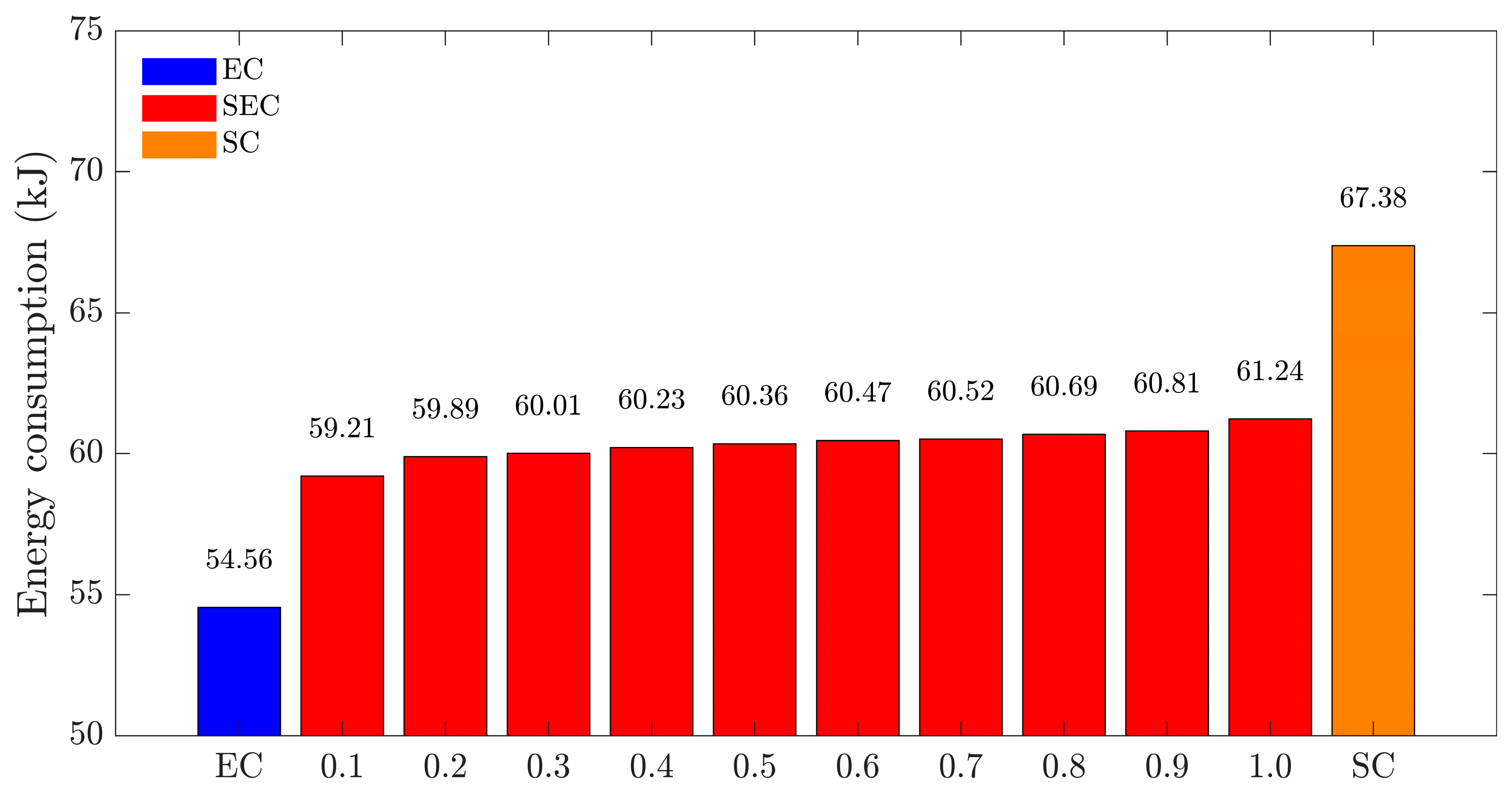
4.3. Case 3:
5. Conclusions
- A compound control strategy, which integrates an adaptive-layer controller, is employed to preserve the advantages of hierarchical control and simultaneously improve energy efficiency.
- The proposed SEC strategy dynamically adjusts the adaptive coefficient based on the vehicle’s battery state and divides the phase plane diagram into three regions according to the evaluation index, which effectively balances lateral stability and energy savings.
- Simulation results demonstrate that the SEC strategy prioritizes energy savings as the battery’s state of charge decreases.
- These findings verify the effectiveness of the proposed adaptive compound controller in achieving a robust balance between lateral stability and energy savings.
Author Contributions
Funding
Institutional Review Board Statement
Informed Consent Statement
Data Availability Statement
Acknowledgments
Conflicts of Interest
References
- Spanoudakis, P.; Tsourveloudis, N.C.; Doitsidis, L.; Karapidakis, E.S. Experimental Research of Transmissions on Electric Vehicles’ Energy Consumption. Energies 2019, 12, 388. [Google Scholar] [CrossRef]
- Zhang, L.; Ding, H.; Shi, J.; Huang, Y.; Chen, H.; Guo, K.; Li, Q. An Adaptive Backstepping Sliding Mode Controller to Improve Vehicle Maneuverability and Stability via Torque Vectoring Control. IEEE Trans. Veh. Technol. 2020, 69, 2598–2612. [Google Scholar] [CrossRef]
- Zhang, X.; Wang, P.; Lin, J.; Chen, H.; Hong, J.; Zhang, L. Real-time nonlinear predictive controller design for drive-by-wire vehicle lateral stability with dynamic boundary conditions. Fundam. Res. 2022, 2, 131–143. [Google Scholar] [CrossRef] [PubMed]
- Zhu, Z.; Tang, X.; Qin, Y.; Huang, Y.; Hashemi, E. A survey of lateral stability criterion and control application for autonomous vehicles. IEEE Trans. Intell. Transp. Syst. 2023, 24, 10382–10399. [Google Scholar] [CrossRef]
- Liang, J.; Feng, J.; Fang, Z.; Lu, Y.; Yin, G.; Mao, X.; Wu, J.; Wang, F. An energy-oriented torque-vector control framework for distributed drive electric vehicles. IEEE Trans. Transp. Electrif. 2023, 9, 4014–4031. [Google Scholar] [CrossRef]
- Yin, G.; Jin, X.; Qing, Z.; Bian, C. Lateral Stability Region Conservativeness Estimation and Torque Distribution for FWIA Electric Vehicle Steering. Sci. China Technol. Sci. 2015, 58, 669–676. [Google Scholar] [CrossRef]
- Qiu, L.; Qian, L.; Zomorodi, H.; Pisu, P. Design and Optimization of Equivalent Consumption Minimization Strategy for 4WD Hybrid Electric Vehicles Incorporating Vehicle Connectivity. Sci. China Technol. Sci. 2018, 61, 147–157. [Google Scholar] [CrossRef]
- Zhuang, W.; Zhang, X.; Yin, G.; Peng, H.; Wang, L. Mode Shift Schedule and Control Strategy Design of Multimode Hybrid Powertrain. IEEE Trans. Control Syst. Technol. 2020, 28, 804–815. [Google Scholar] [CrossRef]
- Shi, K.; Yuan, X.; Huang, G.; Liu, Z.L. Compensation-Based Robust Decoupling Control System for the Lateral and Longitudinal Stability of Distributed Drive Electric Vehicle. IEEE ASME Trans. Mechatron. 2019, 24, 2768–2778. [Google Scholar] [CrossRef]
- Zhang, H.; Zhao, W. Decoupling Control of Steering and Driving System for In-Wheel-Motor-Drive Electric Vehicle. Mech. Syst. Signal Proc. 2018, 101, 389–404. [Google Scholar] [CrossRef]
- Shtessel, Y.; Edwards, C.; Fridman, L.; Levant, A. Sliding Mode Control and Observation; Springer: New York, NY, USA, 2014; ISBN 978-0-8176-4892-3. [Google Scholar]
- Ding, S.; Liu, L.; Zheng, W.X. Sliding Mode Direct Yaw-Moment Control Design for in-Wheel Electric Vehicles. IEEE Trans. Ind. Electron. 2017, 64, 6752–6762. [Google Scholar] [CrossRef]
- Zhao, B.; Xu, N.; Chen, H.; Guo, K.; Huang, Y. Stability Control of Electric Vehicles with In-Wheel Motors by Considering Tire Slip Energy. Mech. Syst. Signal Proc. 2019, 118, 340–359. [Google Scholar] [CrossRef]
- Jiang, Z.; Xiao, B. LQR Optimal Control Research for Four-Wheel Steering Forklift Based-on State Feedback. J. Mech. Sci. Technol. 2018, 32, 2789–2801. [Google Scholar] [CrossRef]
- Wang, Z.; Montanaro, U.; Fallah, S.; Sorniotti, A.; Lenzo, B. A Gain Scheduled Robust Linear Quadratic Regulator for Vehicle Direct Yaw Moment Control. Mechatronics 2018, 51, 31–45. [Google Scholar] [CrossRef]
- Zhao, Y.; Deng, H.; Li, Y.; Xu, H. Coordinated Control of Stability and Economy Based on Torque Distribution of Distributed Drive Electric Vehicle. Proc. Inst. Mech. Eng. Part D J. Automob. Eng. 2020, 234, 1792–1806. [Google Scholar] [CrossRef]
- Ren, B.; Chen, H.; Zhao, H.; Yuan, L. MPC-Based Yaw Stability Control in in-Wheel-Motored EV via Active Front Steering and Motor Torque Distribution. Mechatronics 2016, 38, 103–114. [Google Scholar] [CrossRef]
- Zhang, J.; Sun, W.; Feng, Z. Vehicle Yaw Stability Control via H∞ Gain Scheduling. Mech. Syst. Signal Proc. 2018, 106, 62–75. [Google Scholar] [CrossRef]
- Guo, J.; Luo, Y.; Li, K. An Adaptive Hierarchical Trajectory Following Control Approach of Autonomous Four-Wheel Independent Drive Electric Vehicles. IEEE Trans. Intell. Transp. Syst. 2018, 19, 2482–2492. [Google Scholar] [CrossRef]
- Chen, Y.; Wang, J. Adaptive Energy-Efficient Control Allocation for Planar Motion Control of over-Actuated Electric Ground Vehicles. IEEE Trans. Control Syst. Technol. 2014, 22, 1362–1373. [Google Scholar] [CrossRef]
- Liu, W.; Khajepour, A.; He, H.; Wang, H.; Huang, Y. Integrated Torque Vectoring Control for a Three-Axle Electric Bus Based on Holistic Cornering Control Method. IEEE Trans. Veh. Technol. 2018, 67, 2921–2933. [Google Scholar] [CrossRef]
- De Novellis, L.; Sorniotti, A.; Gruber, P.; Orus, J.; Fortun, J.M.R.; Theunissen, J.; De Smet, J. Direct Yaw Moment Control Actuated through Electric Drivetrains and Friction Brakes: Theoretical Design and Experimental Assessment. Mechatronics 2015, 26, 1–15. [Google Scholar] [CrossRef]
- Kang, J.; Yoo, J.; Yi, K. Driving Control Algorithm for Maneuverability, Lateral Stability, and Rollover Prevention of 4WD Electric Vehicles with Independently Driven Front and Rear Wheels. IEEE Trans. Veh. Technol. 2011, 60, 2987–3001. [Google Scholar] [CrossRef]
- Nam, K.; Fujimoto, H.; Hori, Y. Lateral Stability Control of In-Wheel-Motor-Driven Electric Vehicles Based on Sideslip Angle Estimation Using Lateral Tire Force Sensors. IEEE Trans. Veh. Technol. 2012, 61, 1972–1985. [Google Scholar] [CrossRef]
- De Novellis, L.; Sorniotti, A.; Gruber, P. Wheel Torque Distribution Criteria for Electric Vehicles with Torque-Vectoring Differentials. IEEE Trans. Veh. Technol. 2014, 63, 1593–1602. [Google Scholar] [CrossRef]
- Fujimoto, H.; Harada, S. Model-Based Range Extension Control System for Electric Vehicles with Front and Rear Driving–Braking Force Distributions. IEEE Trans. Ind. Electron. 2015, 62, 3245–3254. [Google Scholar] [CrossRef]
- Chen, J.; Yu, J.; Zhang, K.; Ma, Y. Control of Regenerative Braking Systems for Four-Wheel-Independently-Actuated Electric Vehicles. Mechatronics 2018, 50, 394–401. [Google Scholar] [CrossRef]
- Wang, R.; Hu, C.; Wang, Z.; Yan, F.; Chen, N. Integrated Optimal Dynamics Control of 4WD4WS Electric Ground Vehicle with Tire-Road Frictional Coefficient Estimation. Mech. Syst. Signal Proc. 2015, 60–61, 727–741. [Google Scholar] [CrossRef]
- Zhai, L.; Sun, T.; Wang, J. Electronic Stability Control Based on Motor Driving and Braking Torque Distribution for a Four In-Wheel Motor Drive Electric Vehicle. IEEE Trans. Veh. Technol. 2016, 65, 4726–4739. [Google Scholar] [CrossRef]
- Zheng, H.; Yang, S. A Trajectory Tracking Control Strategy of 4WIS/4WID Electric Vehicle with Adaptation of Driving Conditions. Appl. Sci. 2019, 9, 168. [Google Scholar] [CrossRef]
- Ma, Y.; Chen, J.; Zhu, X.; Xu, Y. Lateral Stability Integrated with Energy Efficiency Control for Electric Vehicles. Mech. Syst. Signal Proc. 2019, 127, 1–15. [Google Scholar] [CrossRef]
- Liu, J.; Zhong, H.; Wang, L.; Chen, H. A Novel Torque Distribution Strategy for Distributed-Drive Electric Vehicle Considering Energy Saving and Brake Stability; SAE Technical Paper 2019-01-0334; SAE International: Warrendale, PA, USA, 2019. [Google Scholar]
- Lin, F.; Qian, C.; Cai, Y.; Zhao, Y.; Wang, S.; Zang, L. Integrated Tire Slip Energy Dissipation and Lateral Stability Control of Distributed Drive Electric Vehicle with Mechanical Elastic Wheel. J. Frankl. Inst. Eng. Appl. Math. 2022, 359, 4776–4803. [Google Scholar] [CrossRef]
- Jing, C.; Shu, H.; Song, Y.; Guo, C. Hierarchical Control of Yaw Stability and Energy Efficiency for Distributed Drive Electric Vehicles. Int. J. Automot. Technol. 2021, 22, 1169–1188. [Google Scholar] [CrossRef]
- Han, Z.; Xu, N.; Chen, H.; Huang, Y.; Zhao, B. Energy-Efficient Control of Electric Vehicles Based on Linear Quadratic Regulator and Phase Plane Analysis. Appl. Energy 2018, 213, 639–657. [Google Scholar] [CrossRef]
- Zhai, L.; Hou, R.; Sun, T.; Kavuma, S. Continuous Steering Stability Control Based on an Energy-Saving Torque Distribution Algorithm for a Four in-Wheel-Motor Independent-Drive Electric Vehicle. Energies 2018, 11, 350. [Google Scholar] [CrossRef]
- Chen, Y.; Wang, J. Design and Experimental Evaluations on Energy Efficient Control Allocation Methods for Overactuated Electric Vehicles: Longitudinal Motion Case. IEEE ASME Trans. Mechatron. 2014, 19, 538–548. [Google Scholar] [CrossRef]
- Pacejka, H.B.; Besselink, I. Tire and Vehicle Dynamics; Butterworth-Heinemann Elsevier: Waltham, MA, USA, 2012; ISBN 978-0-08-097016-5. [Google Scholar]
- Liu, J.; Zhuang, W.; Zhong, H.; Wang, L.; Chen, H.; Tan, C.A. Integrated Energy-Oriented Lateral Stability Control of a Four-Wheel-Independent-Drive Electric Vehicle. Sci. China Technol. Sci. 2019, 62, 2170–2183. [Google Scholar] [CrossRef]
- Inagaki, S.; Kshiro, I.; Yamamoto, M. Analysis on vehicle stability in critical cornering using phase-plane method. In Proceedings of the International Symposium on Advanced Vehicle Control, Tsukuba, Japan, 24–28 October 1994; pp. 287–292. [Google Scholar]
- Shen, S.; Wang, J.; Shi, P.; Premier, G. Nonlinear Dynamics and Stability Analysis of Vehicle Plane Motions. Veh. Syst. Dyn. 2007, 45, 15–35. [Google Scholar] [CrossRef]
- Guo, N.; Zhang, X.; Zou, Y.; Lenzo, B.; Du, G.; Zhang, T. A Supervisory Control Strategy of Distributed Drive Electric Vehicles for Coordinating Handling, Lateral Stability, and Energy Efficiency. IEEE Trans. Transp. Electrif. 2021, 7, 2488–2504. [Google Scholar] [CrossRef]


| Definition | Symbol | Definition | Symbol |
|---|---|---|---|
| vehicle mass | vertical loads at each wheel | ||
| steering angle | gravitational acceleration | ||
| front wheel steering angle | steering ratio | ||
| front right wheel steering angle | rolling friction coefficient | ||
| front left wheel steering angle | wheel rolling inertia | ||
| front to rear axle distance | yaw moment of inertia | ||
| distance from CG to front axle | motor torque on each wheel | ||
| distance from CG to rear axle | motor rotational speed | ||
| front track width | motor efficiency | ||
| rear track width | angel velocity of each wheel | ||
| vehicle longitudinal velocity | wheel rolling radius | ||
| vehicle lateral velocity | road friction coefficient | ||
| yaw rate in vehicle body | cornering stiffness of total tires | ||
| steady-state yaw rate | cornering stiffness of the front tires | ||
| side slip angle in vehicle body | cornering stiffness of the rear tires | ||
| steady-state side slip angle | external yaw moment | ||
| tire longitudinal forces | modified external yaw moment | ||
| tire lateral forces | total longitudinal torque | ||
| total lateral forces of front tires | maximum torque on each wheel | ||
| total lateral forces of rear tires | state of charge |
| Parameter | Value |
|---|---|
| −0.0005 | |
| 0.0372 | |
| −1.1254 | |
| 19.1114 | |
| 0.1079 | |
| 0.0001 | |
| 79.9997 | |
| −1.8113 | |
| 0.7331 |
| L | M | H | ||
|---|---|---|---|---|
| L | VH | H | M | |
| M | H | M | L | |
| H | M | L | VL | |
| Parameter | Unit | Value |
|---|---|---|
Disclaimer/Publisher’s Note: The statements, opinions and data contained in all publications are solely those of the individual author(s) and contributor(s) and not of MDPI and/or the editor(s). MDPI and/or the editor(s) disclaim responsibility for any injury to people or property resulting from any ideas, methods, instructions or products referred to in the content. |
© 2025 by the authors. Licensee MDPI, Basel, Switzerland. This article is an open access article distributed under the terms and conditions of the Creative Commons Attribution (CC BY) license (https://creativecommons.org/licenses/by/4.0/).
Share and Cite
Hua, X.; Xiang, K.; Cheng, X.; Ning, X. An Adaptive Compound Control Strategy of Electric Vehicles for Coordinating Lateral Stability and Energy Efficiency. Appl. Sci. 2025, 15, 3347. https://doi.org/10.3390/app15063347
Hua X, Xiang K, Cheng X, Ning X. An Adaptive Compound Control Strategy of Electric Vehicles for Coordinating Lateral Stability and Energy Efficiency. Applied Sciences. 2025; 15(6):3347. https://doi.org/10.3390/app15063347
Chicago/Turabian StyleHua, Xia, Kai Xiang, Xiangle Cheng, and Xiaobin Ning. 2025. "An Adaptive Compound Control Strategy of Electric Vehicles for Coordinating Lateral Stability and Energy Efficiency" Applied Sciences 15, no. 6: 3347. https://doi.org/10.3390/app15063347
APA StyleHua, X., Xiang, K., Cheng, X., & Ning, X. (2025). An Adaptive Compound Control Strategy of Electric Vehicles for Coordinating Lateral Stability and Energy Efficiency. Applied Sciences, 15(6), 3347. https://doi.org/10.3390/app15063347