Research on the Mechanism and Dynamic Characteristics of Intermittent Failure of Electrical Connectors

Abstract

Aging or damaged electrical connectors always suffer intermittent failures (IFs) during operation. Because there are few quantitative studies on electrical connector intermittent failure mechanisms, the intermittent failures of electrical connectors are difficult to isolate. Therefore, the mechanism and dynamic characteristics of intermittent failure is studied in this paper. Firstly, the degradation process of an electrical connector is analyzed. Secondly, according to electrical contact model, the intermittent failure mechanism caused by vibration is studied. Thirdly, to make a profound study on dynamic behavior of intermittent failure, an intermittent failure dynamic model is proposed, and the behaviors of intermittent failure are analyzed. Finally, a simulation case is conducted to verify the correctness of the intermittent failure mechanism and the effectiveness of the intermittent failure dynamic model.

1. Introduction

With the rapid development of modern industry, laser technology plays an increasingly important role in the fields of material processing [1,2,3], medical treatment [4], sensing technology [5], optical communication [6], military applications, and aerospace [7]. As a high-energy light source that converts electrical energy into light energy, the stability and reliability of lasers are crucial to ensure the performance of the entire system. However, lasers are exposed to harsh conditions such as high temperatures, high voltages, and strong currents during operation, which can lead to damage to laser optics, electrical failures, thermal management problems, and mechanical failures [8]. Intermittent failures of electrical connectors in lasers increase significantly with increasing usage time [9,10]. An intermittent failure (IF) is defined as a failure of an item for a limited period of time, following which the item recovers its ability to perform its tasks without being subjected to any external corrective action [11]. As a kind of intermittent failures, electrical connection intermittent failures may induce false alarms of built-in test (BIT) system [12]. Electrical connection components mainly consist of electrical connector, solder joint, pin and so on. This paper mainly discusses the intermittent failure mechanism of electrical connector. Intermittent failures of each electrical connector will cause operation risk, or, more seriously, a catastrophic accident [13,14].

For the purpose of isolating an intermittent failure, many experts and scholars have carried out relevant studies, which are mainly focused on modeling intermittent failure. Considering the randomness of intermittent failure, a certain number of statistical models of intermittent failure are proposed. To summarize these statistical models [15,16,17,18,19,20,21], the intermittent failures are modeled as a random event with a probability of state transition. Through experimental research, the intermittent failures are found to be closely related to environmental stress. Then, the intermittent failures are modeled as random events with a conditional state transition probability [22], and the intermittent failures’ transfer to fault-free state or permanent fault (PF) state needs to consider the effect of environmental stress [21,23]. By applying these statistical models, the ability to diagnose intermittent failure is improved. However, the validity and accuracy of the statistical model relies on a large number of intermittent failure sample data that are difficult to obtain; therefore, most intermittent failures are still difficult to diagnose and isolate. To improve the ability to diagnose intermittent failure, the intermittent failures must be modeled as a deterministic event instead of a random event. However, there are few research studies on the intermittent failure mechanism as it is difficult to model an intermittent failure as a deterministic event. Thus, the mechanism of intermittent failure is a key issue that should be studied urgently.

This paper mainly discusses the mechanism and dynamic characteristics of intermittent failure of electrical connectors. Among many parameters of electrical connectors, contact resistance is an important parameter that reflects the performance of electrical contact [24,25,26]. Hence, the studies on electrical connector intermittent failure can be concentrated on contact resistance. Compared with other factors, the fretting has the greatest influence on electrical connectors’ contact performance [27]. It is widely acknowledged that fretting is a form of relative sliding with no more than 125 microns of amplitude, and it is the main cause behind the increase in contact resistance. Many research studies on contact resistance have been conducted through experiments [28,29,30,31]. Also, many contact resistance models have been developed, including the Holm model, the Malucci model, and the Groβmann model [32]. Those models performed well in modeling static contact resistance. However, these models are limited to analysis of the mechanism of intermittent failure due to the randomness and dynamics of intermittent failure. To study the mechanism and dynamics of intermittent failure, the effect of degradation and environment stress on intermittent failure are analyzed in this paper. And, the vibrations are selected as the typical environmental stress for investigation.

The rest of this paper is structured as follows. Section 2 provides an analysis of the mechanism of intermittent failure induced by vibration. Section 3 gives parameters for electrical connectors’ intermittent failures, and the dynamic model of intermittent failures is constructed. Section 4 implements a simulation case for model validation. Section 5 concludes this paper and provides some useful remarks.

2. Analysis of the Electrical Connector Intermittent Failure Mechanism

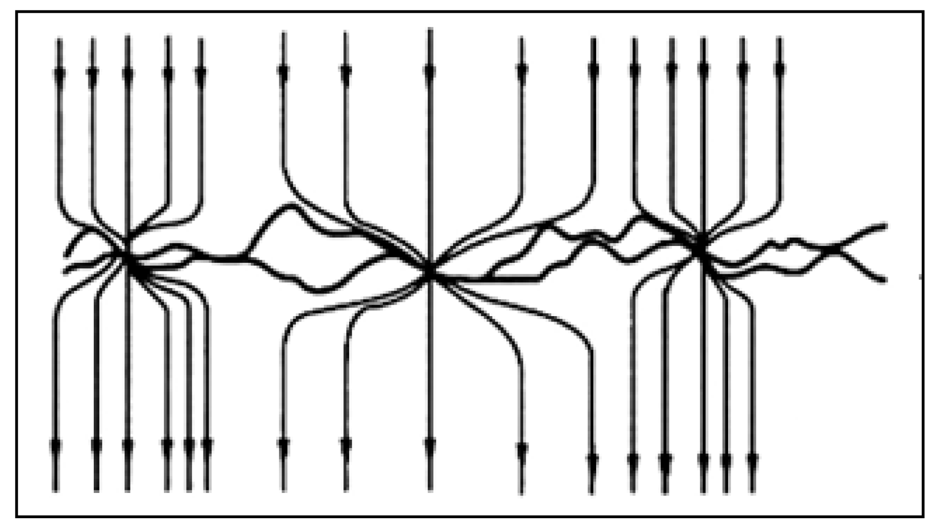
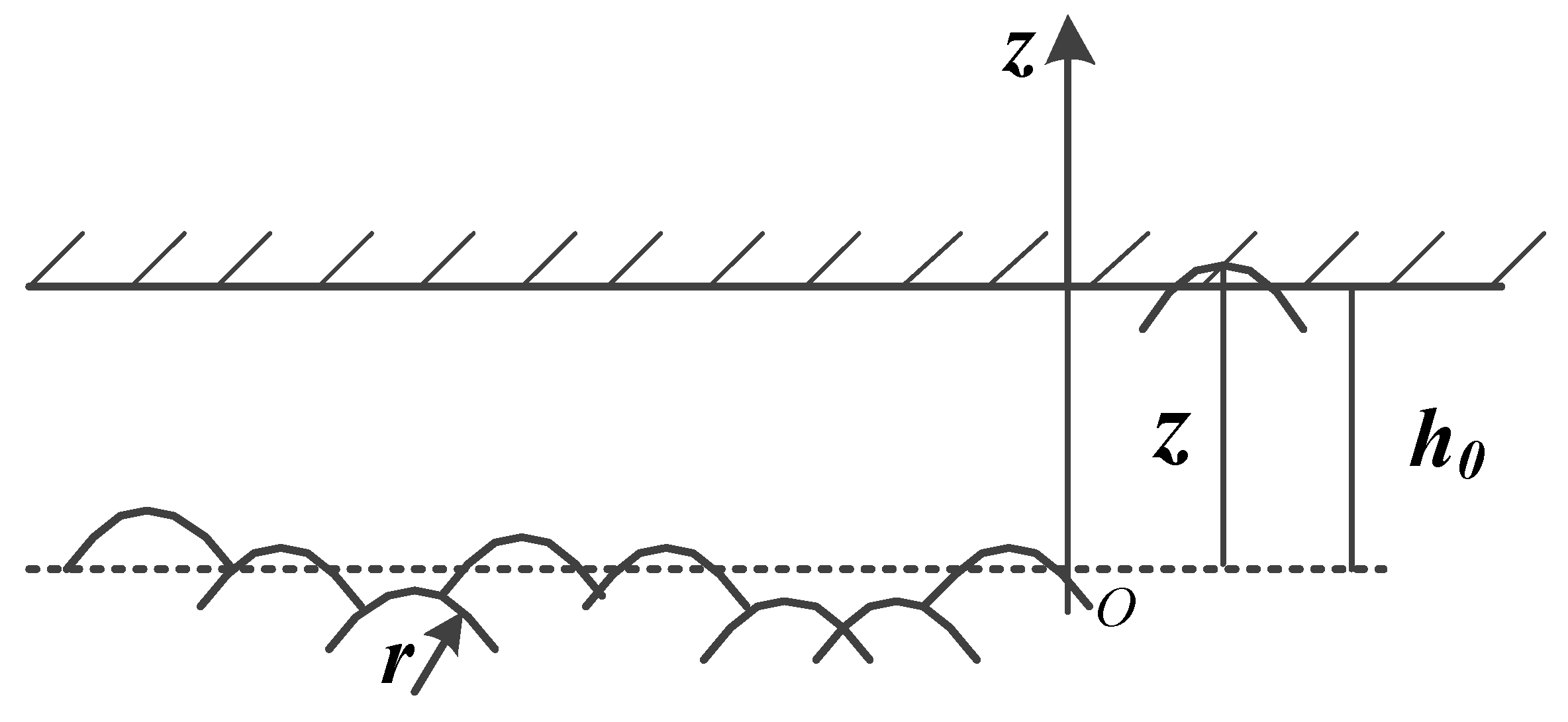
2.1. Contact Resistance Model

It is well known that the contact surface of electrical connector is rough, and there exists many asperities on the surfaces. The two surfaces are contacted and extruded with each other, forming a real contact. Among the real contact area, a small part belongs to the metallic contact area. This metallic contact area where the current can pass through is called contact spot, or “a-spot”. The current will shrink when it passes through “a-spot”, as shown in Figure 1.

The contact resistance is composed of contraction resistance $R_s$ and velamen resistance $R_b$. The contact resistance of the pairs can be expressed as

$$R_c=R_s+R_b$$

(1)

Because each “a-spot” is usually formed after the surface film is destroyed mechanically, the impact of contraction resistance can be ignored. Assuming that the shape of the “a-spot” is a circle, the contact resistance of “a-spot” is expressed as follows:

$$R_s=\left({\rho }_1+{\rho }_2\right)/4a$$

(2)

where ${\rho }_1$ and ${\rho }_2$ represent the electrical resistivity of the contact metal and a denotes the radius of the “a-spot ”. Once the contact material is determined, the contact resistance is mainly determined by the radius of the “a-spot ”.

2.2. Analysis of the Degradation of the Contact Resistance

The common failure mode of the electrical connector includes contact failure, insulation failure, and mechanical failure. The contact failure accounts for the largest number of all electrical connectors’ failures. The reasons for contact failure are as follows:

• Creep and stress relaxation. The creep and stress relaxation both lead to a decrease in the elastic deformation of connectors. According to the Hertz contact theory [32], the conductive area of the contact spot will decrease with the decrease in elastic deformation, resulting in a significant increase in contact resistance.
• Metal migration. The metal migration mainly causes variation in contact area, then contact resistance fluctuates.
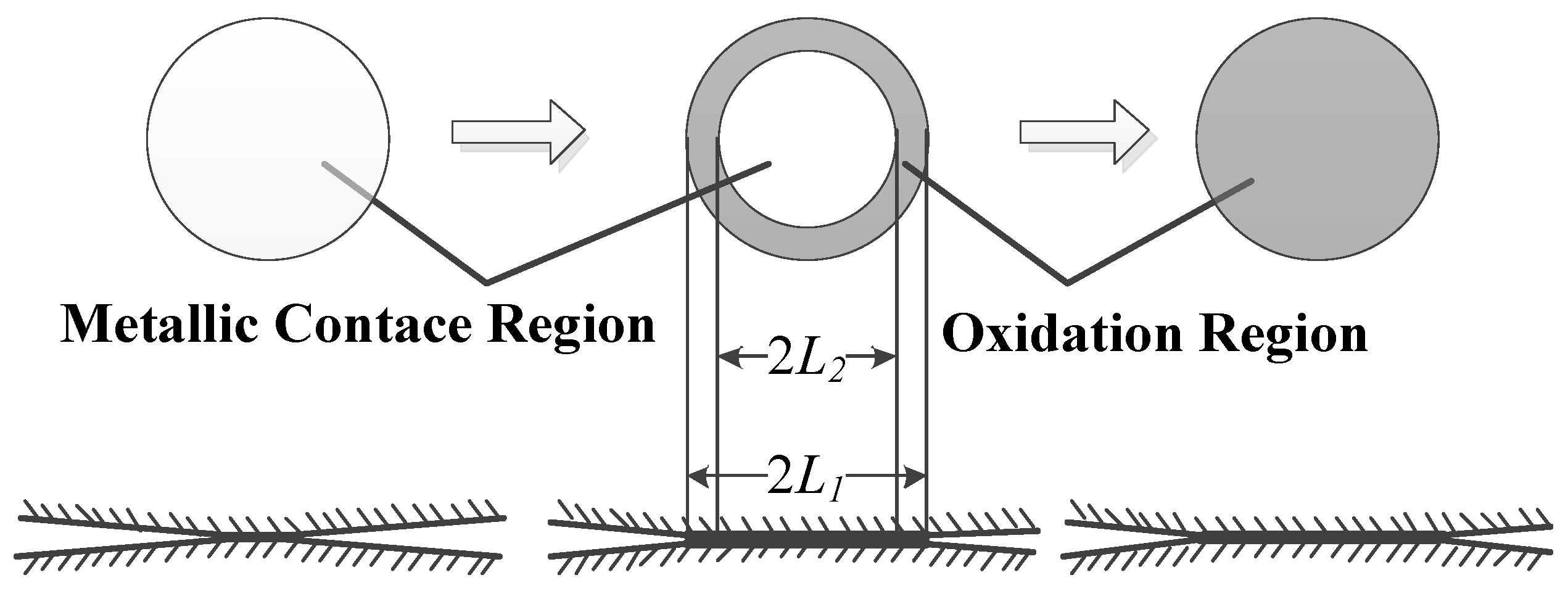
• Oxidation and corrosion. The contact area is easily corroded by oxygen. Thus, the oxidized film, which is composed of an insulating material, will cover the conductive spot gradually. Then, the size of the conductive spot will decrease, and the resistance will increase.

The growth of oxidized film on the surface easily causes contact failure. The growth process is shown in Figure 2. Initially, the film is formed around the conductive spot. As the contact surface is continuously oxidized, the oxidized film accumulates gradually. Finally, the oxidized film, which is made of a nonconductive material, covers the original conductive contact area. When the whole contact surface is covered by oxidized film, the electrical connector fails.

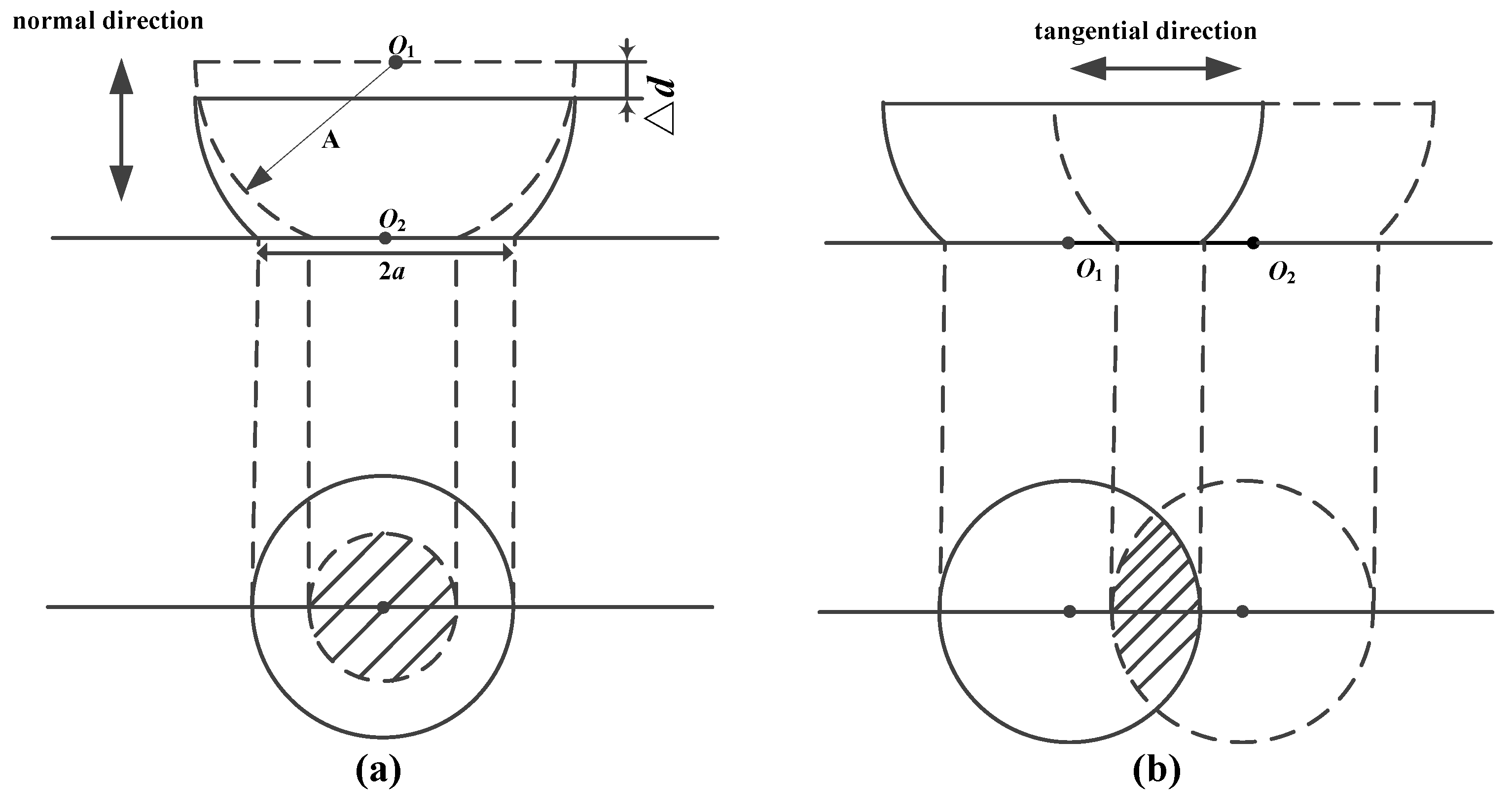
2.3. Electrical Contact Model Considering the Plowing Effect

In this paper, the “a-spot” is assumed to be a contact area that is formed by extrusion of elastic asperity and a rigid plate. Initially, because of the interior or external stress, the asperity would slide on the rigid plate with a micro-amplitude. The relative motion of contact surface leads to the softer metal surface being plowed. On the one hand, the plowing causes oxidation, wear and debris accumulation; on the other hand, the plowing could destroy the original “quasi-metallic” contact film and form a more stable metallic contact.

The region formed by plowing is called the plowing region. Because the “quasi-metallic” film in the plowing region could be destroyed, it can be assumed that the plowing region is the “entire-metallic” contact region. For investigating the influence of the oxidized film, it is assumed that the plowing region is circular and only exists in the rigid plate, and the oxidized film covers the rigid plate only.

The established electrical contact model considering the plowing effect is shown in Figure 3.

In Figure 3a, L₁ denotes the plowing radius at time t, and L₂ denotes the plowing radius at t + Δt. The gray part represents the increment area of the oxidized film during the time interval (t,t + Δt). The white portion within the circle represents the metal contact surface of the rigid plate, and the yellow circle represents the “a-spot ”. With an increasing amount of oxidized film, the metal area of the rigid plate decreases. When the oxidized film entirely covers the “a-spot ”, as shown in Figure 3b, the initial “a-spot ” is replaced by a “metal-film” contact, which manifests as electrical contact failure. The degradation rate could be expressed as dL/dt.

2.4. The Intermittent Failure Mechanism of the Electrical Connector

The intermittent failure mechanism of electrical connectors is complicated and affected by many factors, including the degradation, environmental stress and so on. In particular, the intermittent failure mechanism under the comprehensive effects of thermal cycle and vibration is more difficult to analyze. In this paper, the vibration stress is taken as typical stress for investing the intermittent failure mechanism. Under the action of vibration stress, the two contact pairs of the electrical connector will move away from each other. Considering that the electrical connector may be subjected to vibration stress from various directions during operation, the direction of relative displacement is random. The relative motion of two contact pairs is considered to be normal motion and tangential motion in this paper, as shown in Figure 4a and Figure 4b, respectively.

In Figure 4, the asperity of solid line indicates the initial position, and the asperity of dotted line indicates the displacement boundary. The circular area within the solid line circle and dotted line circle represents the change range of contact area during movement.

It can be considered that the area outside the solid circular is completely covered with the insulating film layer. The dashed area is metallic contact. According to Hertz contact theory [32], the relationship between the contact radius a and the contact depth d is d = a²/2A, where A represents the radius of curvature of the asperity. Let Δd be the normal displacement; then, the radius of the dotted circle in Figure 4a is

$$a_f=\sqrt{a^2-2A\Delta d}$$

(3)

Combining Equations (2) and (3), the maximum value of contact resistance R_s caused by relative displacement is

$$R_s=\left({\rho }_1+{\rho }_2\right)/4\sqrt{a^2-2A\Delta d}$$

(4)

According to Equation (4), it can be seen that the contact resistance will increase with the increasing of the displacement Δd. If the relative displacement is large enough, the contact resistance will exceed the failure threshold, leading to failure. Further, once the external stress disappears, the asperity will return to its initial position due to the restoring force of the elastic part of the electrical connector. Then, the failure disappears and the whole process manifests as an intermittent failure.

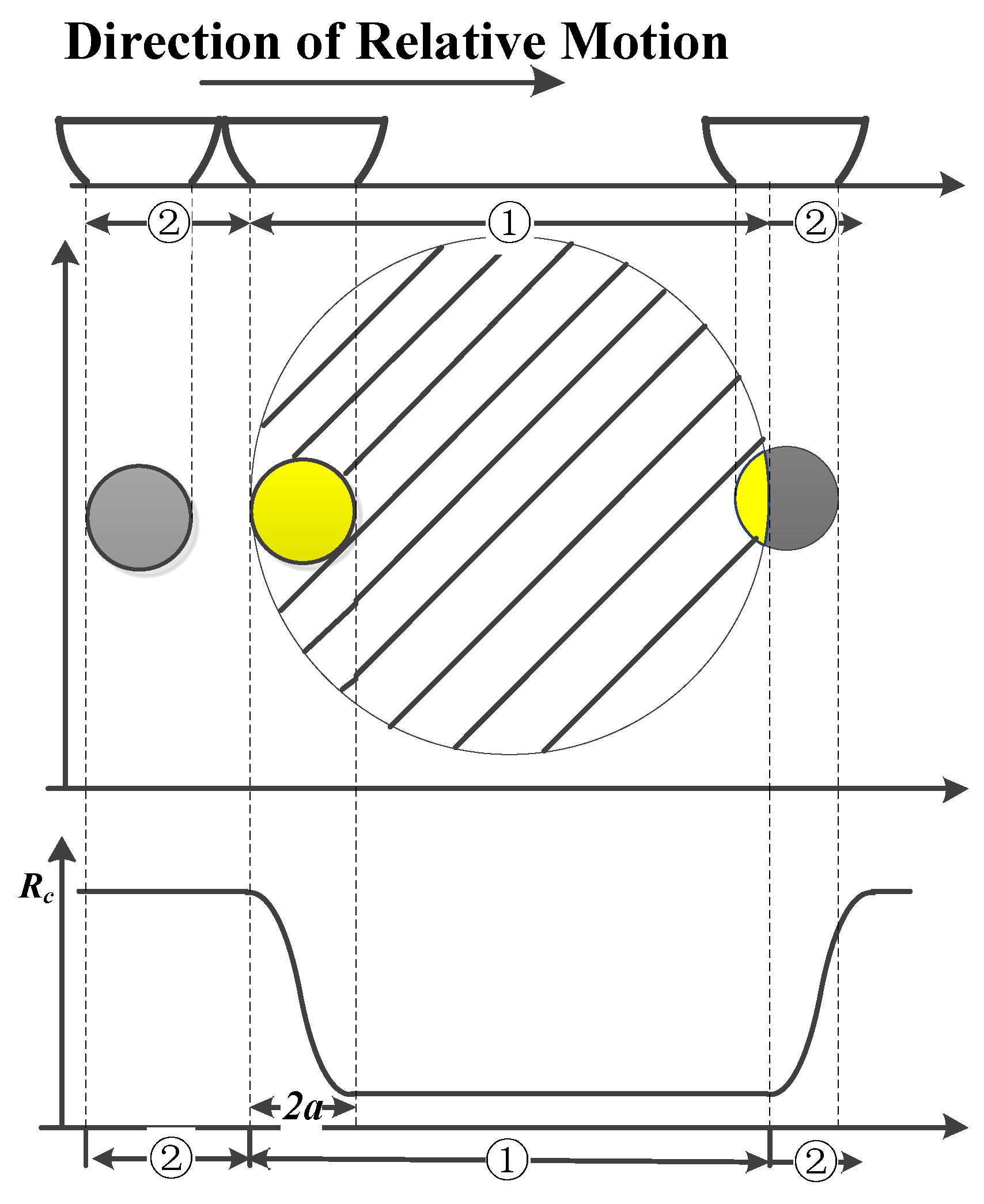
2.5. Analysis of the Mechanism of Electrical Connector Intermittent Failure Induced by Vibration

In practice, the vibration is one of the primary factors that could cause the relative movement of the contact pairs. To investigate the electrical connector intermittent failure induced by vibration, the dynamic model of electrical connector under vibration is constructed, as shown in Figure 5.

According to Figure 5, the differential equation of the dynamic model is obtained as follows:

$$m_3{\ddot{z}}_c+2c_4{\dot{z}}_c+2k_4{z}_c=F\left(t\right)-\left(m_3-m_4\right){\ddot{z}}_4-m_1{\ddot{z}}_1-m_2{\ddot{z}}_2-2k_2\left(z_2-z_4\right)$$

(5)

The expression of $z_c$ is a sine or cosine wave when the vibration equation F(t) follows a sine or cosine wave. The amplitude of the relative displacement $z_c$ is maximized if the electrical connector is forced to vibrate at the resonance frequency. Let z_c(t) = Z_csin2πft, where $Z_c$ denotes the amplitude of $z_c$.

By analyzing the mechanism of intermittent failures induced by vibration is shown in Figure 6, and the contact resistance curve of a contact spot under sinusoidal vibration can be calculated.

In Figure 6, the shaded region of the larger circle refers to the plowing region, denoted by ①. The outer region refers to the oxidized region, denoted by ②. The smaller circle represents the “a-spot ”. The conductivity of the contact spot depends on the distribution of oxidized film on the rigid plate and the relative position of the asperity and the rigid plate.

Assuming that the displacement direction of the asperity remains consistent with the arrowhead, the curve of the contact resistance R_c could be plotted in Figure 6. Initially, the asperity comes into contact with the rigid plate in region ②, forming a “metal-oxide” contact spot that is nonconductive. As the asperity slides to region ①, the “metal-oxide” contact spot turns to an “entire-metallic” contact, which is conductive. If the asperity continues to reciprocate with the rigid plate, then the contact resistance value fluctuates. Once the level of vibration stress is high enough, intermittent failure may occur, and, the higher the vibration stress is, the higher the probability is for electrical connector intermittent failure.

The dynamic behavior of electrical connector intermittent failure in a reciprocating cycle is analyzed as follow. Assuming that the asperity is completely within region ① at time 0 and, considering the randomness of direction of plowing, the relative position between asperity and rigid plate is random. Let the distance from the center of the asperity to the left border of region ① be n and the distance to the right border of region ① be m, n > m, as shown in Figure 7.

According to the different amplitudes of reciprocating motion Z_c, a simple discussion of the dynamic behaviors of intermittent failure during a reciprocating cycle is given below.

Case 1: When Z_c < m, the asperity is always within region ① during a reciprocating cycle, and the contact resistance is stabilized at a lower value.

Case 2: When m < Z_c < n, the asperity slides to region ② from the right boundary of the region ①; the intermittent failure could be observed only once.

Case 3: When n < Z_c, the asperity slides to region ② from both the left and right boundaries of region ①; the intermittent failure could be observed twice.

The curve of contact resistance is shown in Figure 8.

Figure 8 shows that the duration and numbers of intermittent failure shows different behaviors under different conditions. To investigate the evolution of intermittent failure dynamic behaviors, the dynamic model of intermittent failure should be studied.

3. Analysis of Intermittent Failure Dynamic Characteristics

3.1. G-W Model

Milenko Braunovic [32] study the reliability and performance of electrical contact using G-W model, which is assumed that all asperities have the same radiuses of curvature r, and the contact surfaces are equivalent to the contact of a smooth rigid plane and a rough surface, as shown in Figure 9 [33].

Generally, the heights of the asperities are modeled as a Gaussian distribution which is given by

$$\phi \left(z\right)={\left({\displaystyle \frac{1}{2\pi {\sigma }^2}}\right)}^{1/2e^{-{\displaystyle \frac{z^2}{2{\sigma }^2}}}\hspace{0.17em}}$$

(6)

where z denotes the height of the asperity and σ denotes the root mean square of z. According to the G-W model and the dynamic resistance of a single “a-spot”, the dynamic model of the contact resistance with multiple a-spots could be constructed.

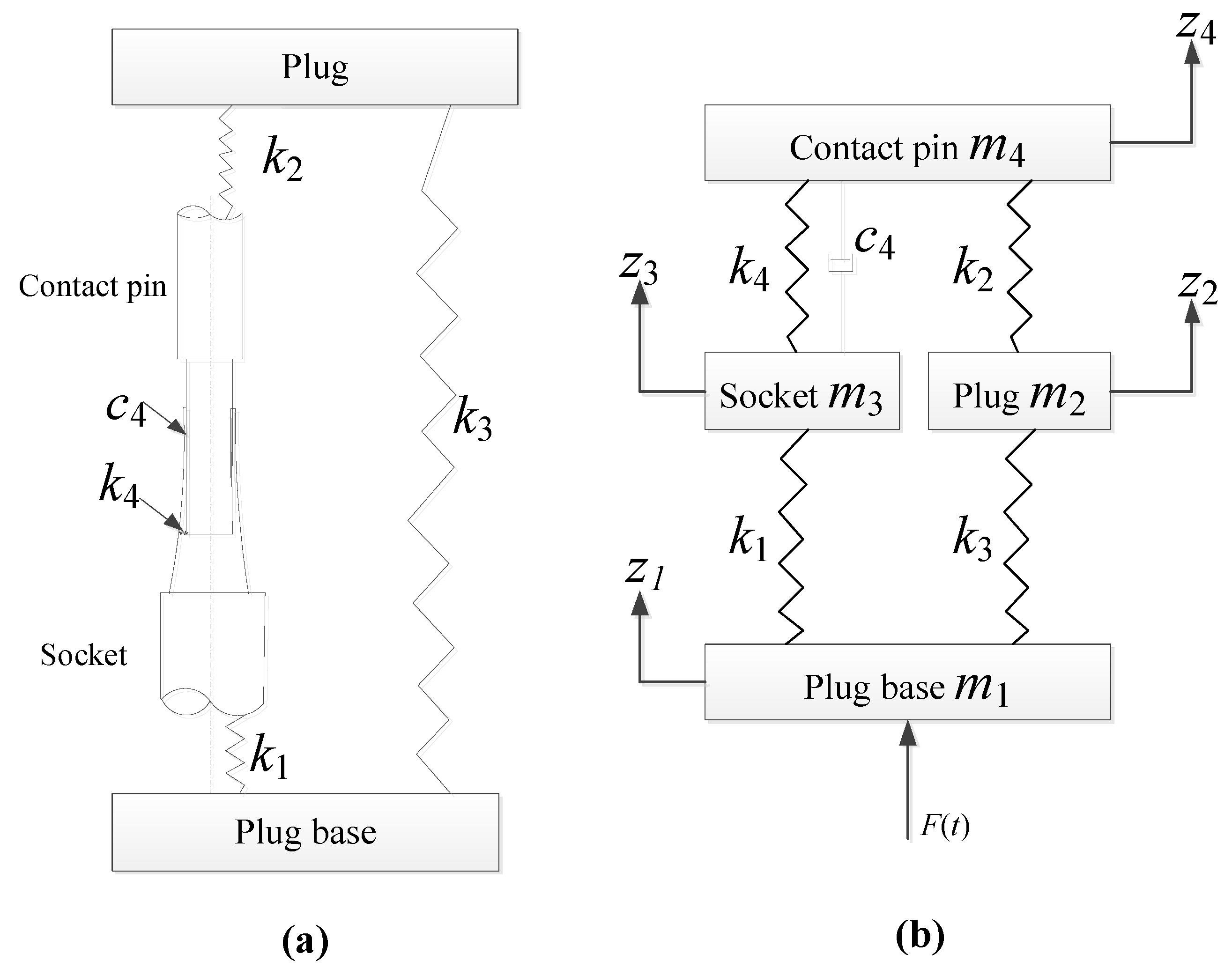
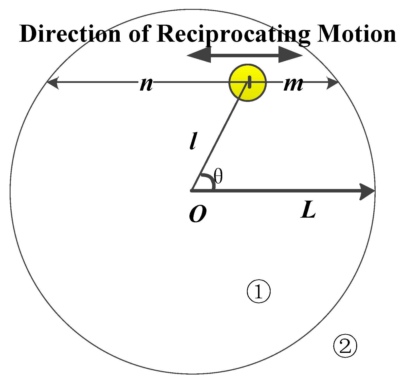
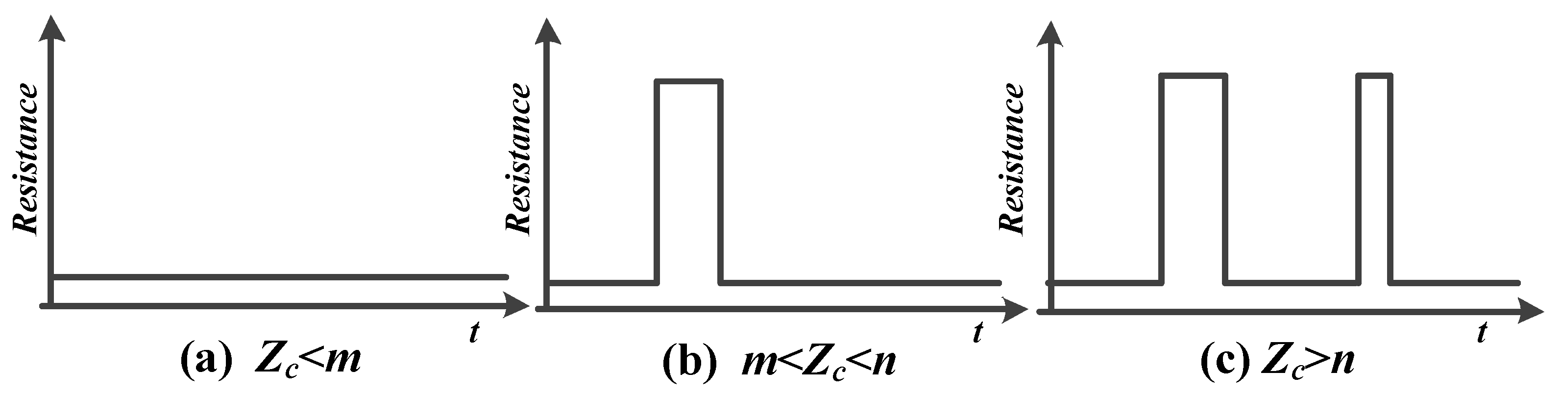
3.2. Parameter Framework of the Dynamic Model of Intermittent Failure

To construct the dynamic model for intermittent failure, the parameter framework of intermittent failure should be proposed firstly. According to the mechanism of intermittent failure, it is clear that the dynamic behaviors of intermittent failure are affected by environmental stress, degradation, and other random factors. In this paper, the parameter framework is divided into input parameters and output parameters.

The input parameters consist of relative motion parameters, degradation parameters, and other random parameters. The key parameters of relative motion are amplitude Z_c and frequency f. The key parameter of degradation is the plowing region radius L. With the oxidized film increasing, L decreases gradually. The other random parameters include the size and position of the “a-spot”. The output parameters consist of the number of occurrences and the duration of intermittent failures.

3.3. Dynamic Model of Intermittent Failure

To analyze the dynamic characteristics of intermittent failure, it is necessary to determine the initial state of the contact surface first. The initial state of the contact consists of the mean radius of the “a-spot”, the relative position between the asperity and the rigid plate, and so on.

The mean radius of the conductive spots is denoted by $\overline{a}$. Before calculating the value of $\overline{a}$ the ratio of the “a-spot” area to the total contact area and the ratio of the number of conductive spots to the total number of asperities or contact spots are proposed in this paper, denoted by $\epsilon$ and $\eta$, respectively. $\epsilon$ and $\eta$ are given by

$$\epsilon =A_c/A$$

(7)

$$\eta =N_c/N$$

(8)

where A_c and N_c denote the total conductive area and the total number of conductive spots, respectively, and A and N denote the total contact area and the total number of actual contact asperities, respectively.

Let the total number of asperities be N₀; thus, N and A can be deduced from the G-W model.

$$N={\displaystyle {\int }_{h_0}^{\infty }{N}_0\phi \left(z\right)}dz$$

(9)

$$A={\displaystyle {\int }_{h_0}^{\infty }{N}_0\phi \left(z\right)\pi r\left(z-h_0\right)}$$

(10)

where $\phi \left(z\right)$ represents the probability density function (PDF) of the asperity height, h₀ represents the average height of the rough surface, and r represents the radius of asperities.

Combining Equations (9) and (10), $\overline{a}$ is derived as follows.

$$\overline{a}=\sqrt{{\displaystyle \frac{A_c}{\pi \cdot N_c}}}=\sqrt{{\displaystyle \frac{{\displaystyle {\int }_{h_0}^{\infty }N\phi \left(z\right)\pi r\left(z-h_0\right)dz}}{{\displaystyle {\int }_{h_0}^{\infty }N\phi \left(z\right)dz}}}{\displaystyle \frac{\epsilon }{\eta }}}$$

(11)

The position of each “a-spot” is related to its corresponding plowing region and is represented using polar coordinates, denoted by (l_i, θ_i), i = 1, 2… N_c. where l_i denotes the distance between the ith center of conductive spot and its corresponding center of the plowing area. θ_i denotes the relative angle between the ith center of conductive spot and its corresponding center of the plowing area. It is assumed that l_i and θ_i both follow a uniform distribution.

$$f_{\theta }\left(y\right)=\left\{\begin{array}{c}\begin{array}{cc}1/2\pi & y\in \left[0,2\pi \right]\end{array}\\ \begin{array}{cc}0& \mathit{\text{otherwise}}\end{array}\end{array}\right.$$

(12)

$$f_l\left(x\right)=\left\{\begin{array}{c}\begin{array}{cc}1/L& x\in \left[0,L\right]\end{array}\\ \begin{array}{cc}0& \mathit{\text{otherwise}}\end{array}\end{array}\right.$$

(13)

where L denotes the radius of the plowing region.

The initial contact resistance could be calculated using the initial parameters mentioned above. Then, the contact resistance can be calculated via an iterative algorithm.

Ignoring the transition effect resulting from the size of the spot, each conductive spot resistance only has two states: one state is the low-resistance state R_l, which represents the conductive state; the other state is the high-resistance state R_h, which denotes the nonconductive state. R_l and R_h both can be calculated according to Equation (2); however, when calculating R_h, ρ_1, or ρ₂ represent the resistivity of the oxidized film material.

Considering the parallel structure of each conductive spot, it is necessary to calculate the contact resistance R_ci (i = 1, 2... N_c) of each conductive spot at the current time. Using the relative motion equation z_c(t), R_ci is given as follows:

$$R_{ci}\left(t\right)=\left\{\begin{array}{l}{R}_l\hspace{0.33em}\hspace{0.33em}\hspace{0.33em}\hspace{0.33em}\hspace{0.33em}-L<l_i\cos {\theta }_i+z_c\left(t\right)<L\\ R_h\hspace{0.33em}\hspace{0.33em}\hspace{0.33em}\hspace{0.33em}\hspace{0.33em}\hspace{0.33em}\hspace{0.33em}\hspace{0.33em}\hspace{0.33em}\hspace{0.33em}\mathrm{otherwise}\end{array}\right.$$

(14)

The contact resistance R_c at time t is derived as follows.

$$R_c\left(t\right)={\displaystyle \frac{1}{{\displaystyle \sum _{i=1}^{N_c}1/R_{ci}(t)}}}$$

(15)

Let Rth be the predetermined fault threshold. If the value of $R_c\left(t\right)$ is less than $R_{th}$, then the electrical connector is fault-free; otherwise, failure occurs. The dynamic characteristics of intermittent failures proposed in this paper mainly consist of occurred numbers denoted by $N_I$, duration in due time denoted by $D_I$, and the average numbers in due time denoted by $\overline{N_I}$ and the average duration denoted by ${\overline{D}}_I$.

According to parameters framework of intermittent failure dynamic model, the intermittent behavior in electrical connector can be described quantitatively. The above modeling process can be summarized as follows:

Step 1: Set the initial electrical contact state parameters, including $z_c\left(t\right)$, $\overline{a}/R_{ci}$,$\left(l_i,{\theta }_i\right)$, $L$, $N_c$ and so on.

Step 2: According to (15) and $z_c\left(t\right)$, calculate the initial electrical contact resistance R_c(0);

Step 3: Let $t=t+\Delta t$; calculate $R_c\left(t\right)$. If $t$ reaches the cut-off time, then go to step 4; otherwise, repeat step 3;

Step 4: Obtain the statistics $N_I$ and $D_I$ according to $R_{th}$;

Step 5: Extract the dynamic characteristics of intermittent failure using Equations (14) and (15).

4. Simulation Case

The dynamic behaviors of intermittent failures are analyzed in this section through simulation. The dynamic model proposed in this paper involves microscopic parameters which are difficult to directly observe and acquire. So, a set of simulation parameters for electrical connectors considering vibration stress are selected from reference [34,35], as shown in

Table 1. Simulation parameters.

Parameter	Value
$\overline{a}$	1.45 μm
Nc	7
L	10 μm
l	U(0,L)
θ	U(0,2π)
Zc	16 μm
f	100 Hz
tc	10 μs
Δt	10−3 μs
Rth	0.8 Ω

Notes: The notation U(,) is the symbol of the uniform distribution function.

.

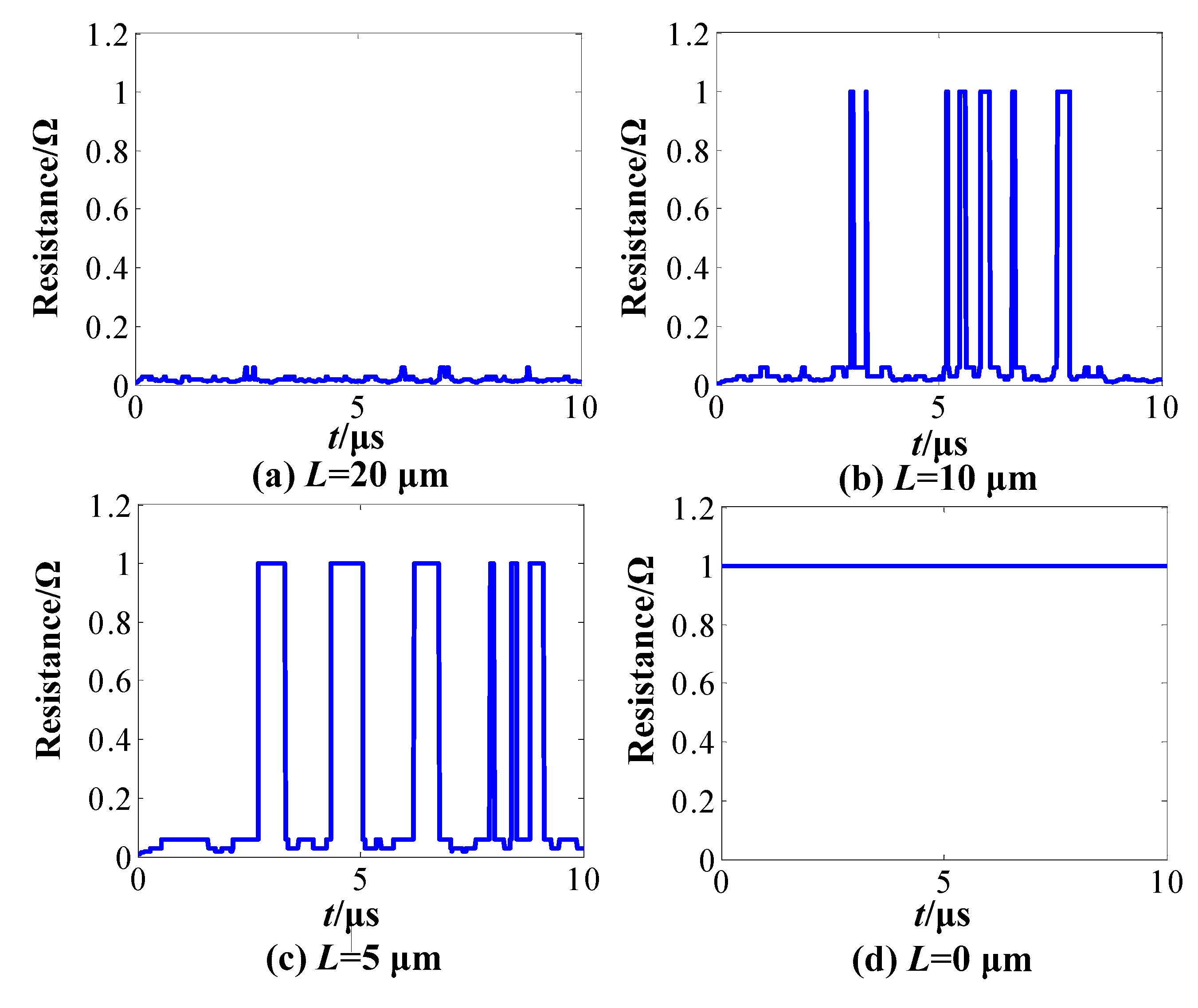
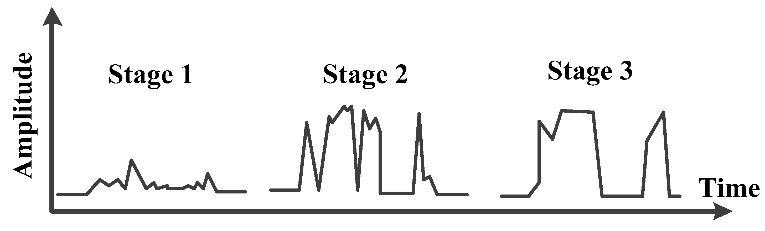
4.1. Dynamics of Intermittent Failure Under Different Degradation Stages

According to the electrical contact model constructed in Section 2, the plowing radius L could be used to represent the degradation stage of electrical connectors.

Let the plowing radius be initially L = 20 μm. Next, take L = 20 μm, 10 μm, 5 μm, and 0 μm separately, to simulate the different degradation stages. The other parameters remain as Table 1, and the contact resistance curve under different degradation stages is shown in Figure 10.

It is seen that, with the continuous growth of the oxidized film, the duration and numbers of intermittent failures both increase progressively. When L decreases to 0, that is, the contact surface is completely covered by oxidized film, the intermittent failures evolve to permanent failure, as shown in Figure 10d. The three phases of dynamic evolution for intermittent failures shown in Figure 10a–c are consistent with the dynamic behaviors of intermittent failures proposed in reference [21], as shown in Figure 11.

4.2. Dynamics of Intermittent Failure Under Different Contact Pressures

The creep and stress relaxation of the electrical connector elastic socket will cause a loss of contact pressure. According to Hertz theory and the G-W model, the decrease in the contact pressure directly leads to decreases in the contact area. The relationship between the total contact area A and the contact pressure $F_N$ proposed in reference [19] is expressed as

$${\displaystyle \frac{A}{F_N}}\approx {\left({\displaystyle \frac{r}{\sigma }}\right)}^{1/2}{\displaystyle \frac{\mathrm{ 3.3}}{E^{*}}}$$

(16)

where E^* denotes the equivalent Young modulus, r denotes the deformation of asperities, and σ denotes the relative curvature.

According to the positive correlation between the total contact area A and the number of contact spots $N$, the correlation between contact pressure F_N and conductive spots number $N_c$ can be expressed as.

$$N_c\propto {\left({\displaystyle \frac{R}{l}}\right)}^{1/2}{\displaystyle \frac{\mathrm{ 3.3}}{E^{*}}}\eta F_N$$

(17)

where η is constant and R denotes the curvature radius of asperities.

There is a positive correlation between F_N and N_c according to Equation (18). Thus, it is reasonable to simulate the different contact pressure through modulating the number of conductive spots.

Let N_c be 10 and 1 separately, and the other parameters remain as in Table 1; the simulation results are the contact resistance curves shown in Figure 12a,b.

It is seen that the duration of intermittent failure under 1 conductive spot is greater than the duration of intermittent failure under 10 conductive spots, and the number of intermittent failures under 1 conductive spot is less than the number of intermittent failures under 10 conductive spots.

To further analyze the dynamic behaviors of intermittent failure, large amounts of simulations are conducted under the same condition. In the simulations, the number of conductive spots is increased from 1 to 10 with the step length of 1. The average number of intermittent failures $\overline{N_I}$ and the average duration of intermittent failures ${\overline{D}}_I$ vary with the number of conductive spots, as shown in Figure 13a and Figure 13b, respectively.

From Figure 13, with an increase in the number of conductive spots, the average number and duration of intermittent failure are generally decreasing. Considering the positive correlation between the number of conductive spots and the contact pressure, it can be concluded that the increase in contact pressure can resist external stress, thereby reducing the probability of intermittent failure. In contrast, with the creep and stress relaxation of the elastic component increasing, the electrical connectors are more likely to suffer intermittent failure. The conclusion that an increase in contact pressure can improve the electrical connector reliability is consistent with the conclusions mentioned in reference [13].

By comparing Figure 12 and Figure 13, it can be observed that there is no strong correlation between the number of intermittent faults and Nc. This is because the change in the number of conductive spots leads to changes in both aspects. On the one hand, the increase in the number of conductive spots indicates that the electrical contact performance is good. On the other hand, the increase in the number of conductive spots is also likely to cause fluctuations in contact resistance, especially loading the condition of vibration stress. Therefore, the relationship between the number of conductive spots and the number of intermittent faults still needs further study.

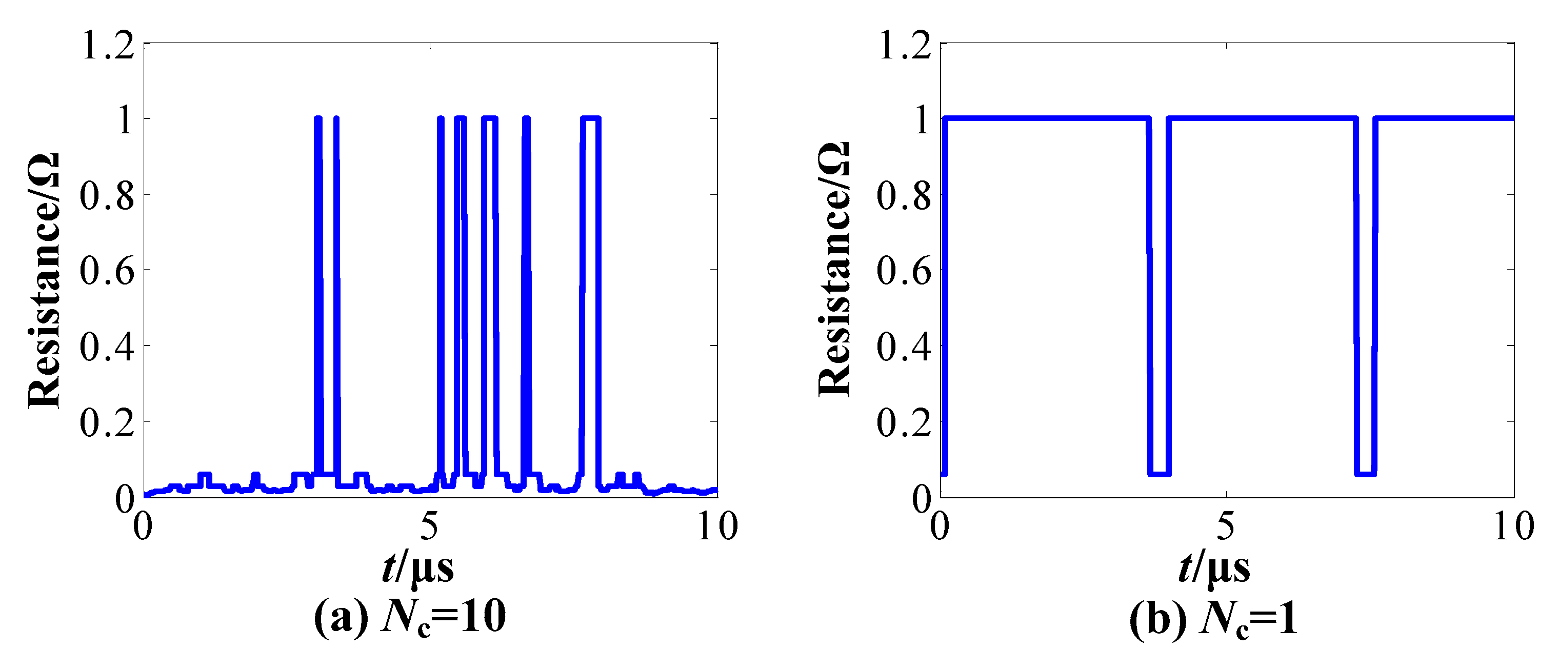
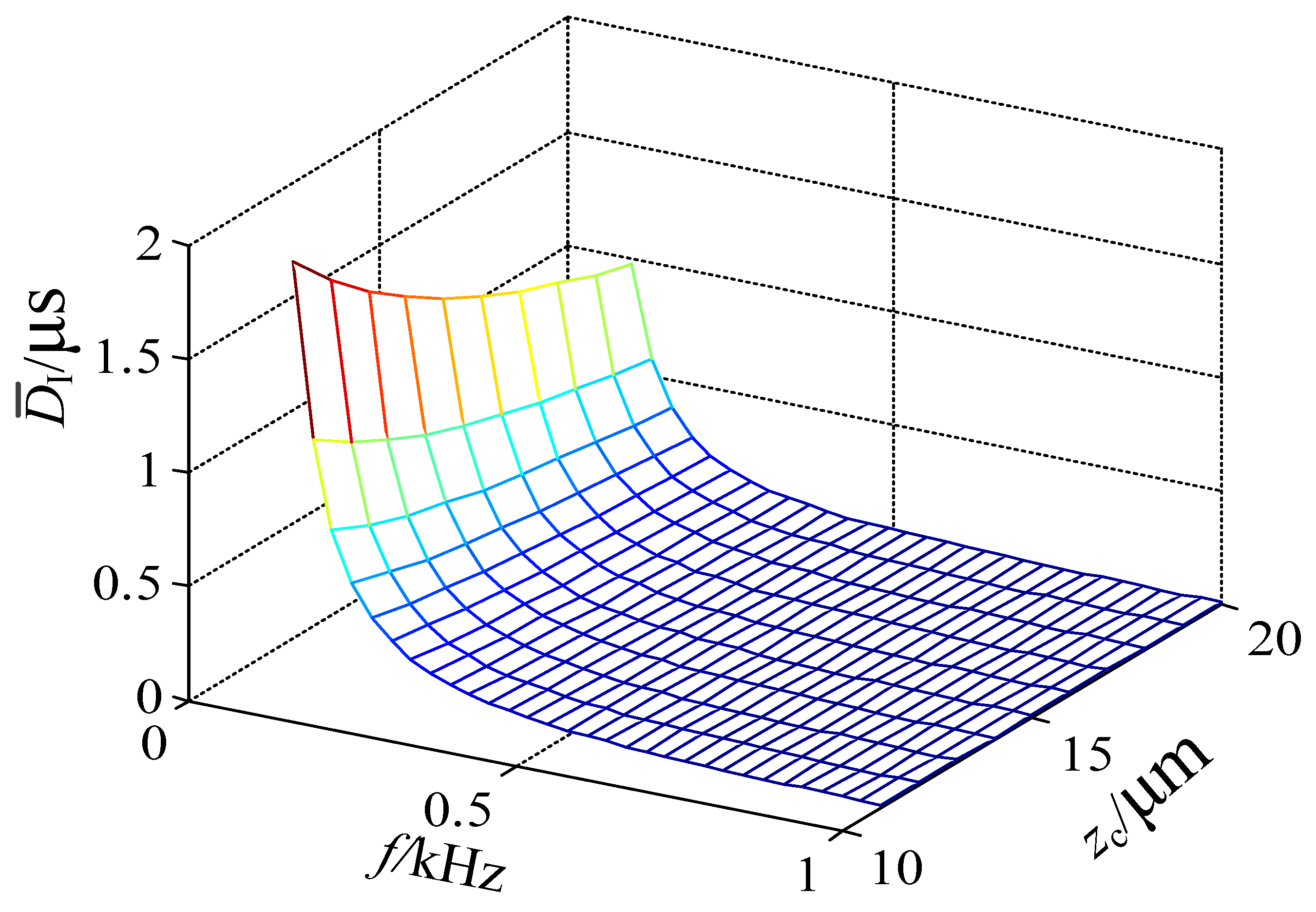
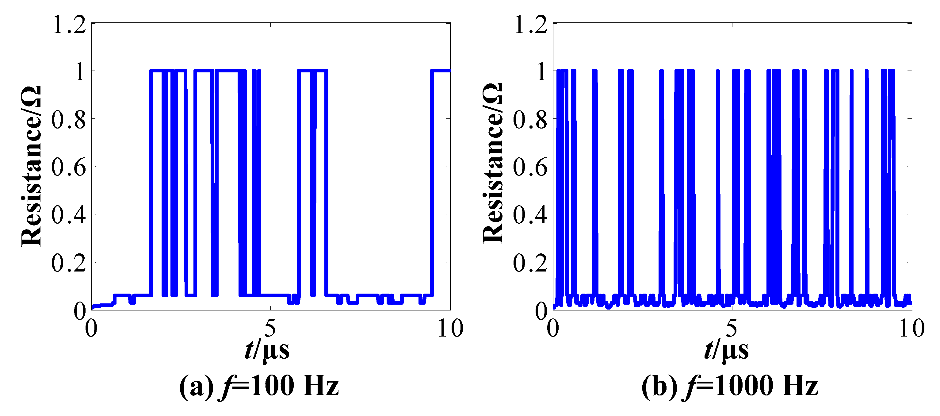
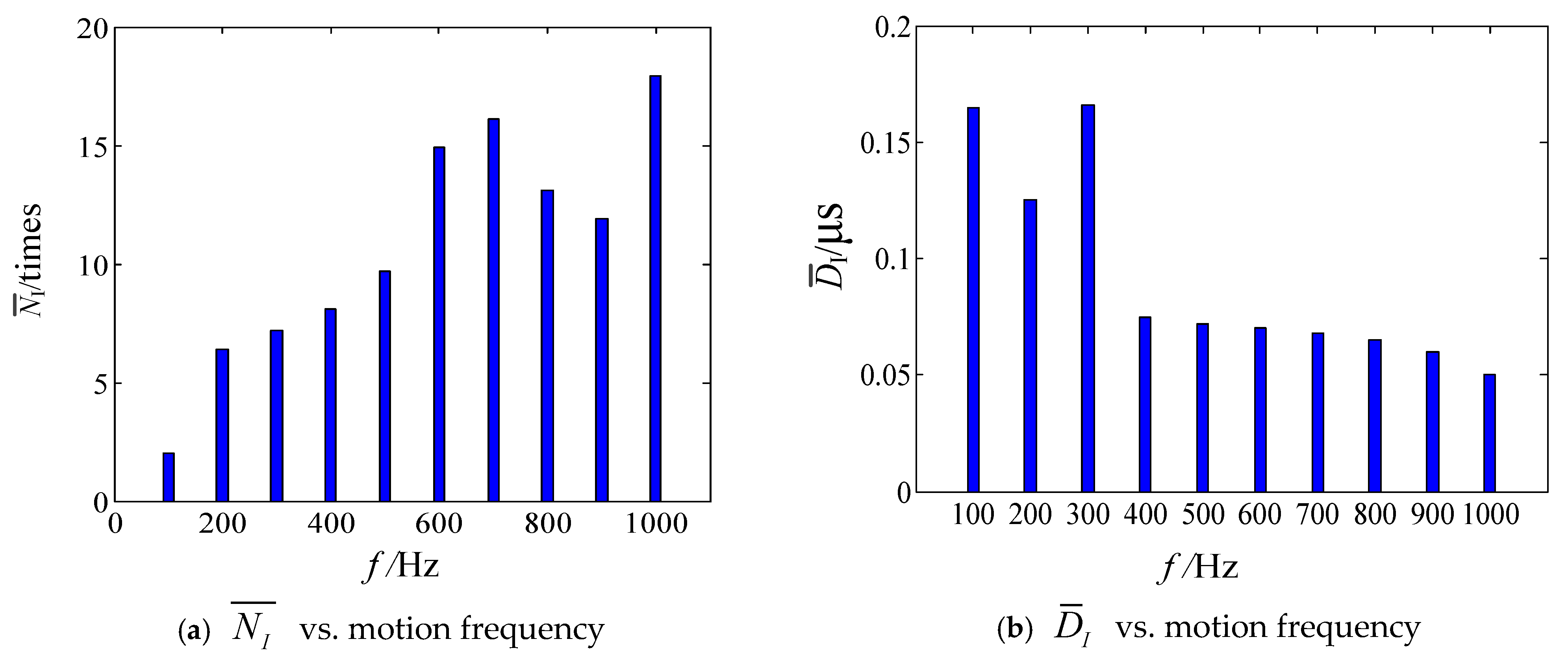
4.3. Dynamics of Intermittent Failure Under Different Relative Motion Parameters

In the simulation, the effects of amplitude $Z_c$ and frequency $f$ on intermittent failures are investigated. The number of intermittent failures N_I and the duration of intermittent failures $D_I$ during the simulation time interval $\left(0,t\right)$ are expressed as

$$N_F=2tf$$

(18)

$$D_F={\displaystyle \frac{\pi -\arccos \frac{m}{A}-\arccos \frac{n}{A}}{\pi f}}$$

(19)

According to Equations (18) and (19), ${\overline{D}}_F$ can be expressed as

$${\overline{D}}_F={\displaystyle \frac{D_F}{N_F}}={\displaystyle \frac{\pi -\arccos \frac{m}{A}-\arccos \frac{n}{A}}{2\pi f^{2}t}}$$

(20)

According to Equation (20), the three-dimensional correlation surface of amplitude-frequency-duration can be plotted, as shown in Figure 14.

Additionally, the average duration ${\overline{D}}_I$ decreases with the increase in $f$. As shown in Figure 14, ${\overline{D}}_I$ decreases rapidly with the increase in f before 0.3 kHz, and then the descending trend is slowed down with the decrease in $f$. Moreover, ${\overline{D}}_I$ is found to increase with the amplitude $Z_c$. In the simulation, the amplitude $Z_c$ is fixed, while the frequency $f$ is taken as the single factor variable for investigating the dynamic characteristics of intermittent failure.

The other parameters are set as shown in Table 1 and frequency f is set to 100 Hz and 1000 Hz separately. Thus, the contact resistance curves under different movement frequencies are shown in Figure 15.

The duration of intermittent failure under 100 Hz is found to be longer than the duration of intermittent failure under 1000 Hz. and number of intermittent failures under 100 Hz is less than number of intermittent failures under 1000 Hz.

To further analyze the dynamic characteristics of intermittent failures, a large number of simulations are implemented under the same condition. In the simulations, the movement frequency $f$ is increased from 100 Hz to 1000 Hz at the step of 100 Hz. The average number of intermittent failures ${\overline{N}}_I$ and the average duration of intermittent failure ${\overline{D}}_I$ as functions of frequency f are shown in Figure 16a and Figure 16b, respectively.

From the simulation results, it can be seen that the average number and the average duration of the intermittent failure under the frequency $f$ are consistent with the theoretical analysis. The effects of the movement amplitude $Z_c$ on intermittent failure dynamic behaviors could be analyzed using the same approach as that for the effects of movement frequency.

5. Conclusions

The aim of this paper was to analyze the mechanism and dynamic behaviors of electrical connectors’ intermittent failure. The primary contributions are summarized as follows:

Based on the G-W model, a degradation model for electrical connectors is constructed and two modes of intermittent failure of electrical connectors caused by vibration stress are analyzed. Considering various factors that induce intermittent failures, a framework for dynamic characteristic parameters of intermittent failures of electrical connectors is established. By using numerical simulation methods, the influences of the degradation degree, contact pair pressure, and relative motion direction on the dynamic characteristics of intermittent failures are studied, respectively. The simulation results show that, with the degradation of electrical connectors, the probability of intermittent failures increases gradually until complete failure. With the creep and stress relaxation of the elastic component, the electrical connectors are more likely to suffer intermittent failure.

References

1. Arulvel, S.; Jain, A.; Kandasamy, J.; Singhal, M. Laser processing techniques for surface property enhancement: Focus on material advancement. Surf. Interfaces 2023, 42, 103293. [Google Scholar]
2. Gu, D.; Shi, X.; Poprawe, R.; Bourell, D.L.; Setchi, R.; Zhu, J. Material-structure-performance integrated laser-metal additive manufacturing. Science 2021, 372, eabg1487. [Google Scholar] [CrossRef] [PubMed]
3. Wei, C.; Zhang, Z.; Cheng, D.; Sun, Z.; Zhu, M.; Li, L. An overview of laser-based multiple metallic material additive manufacturing: From macro-to micro-scales. Int. J. Extrem. Manuf. 2020, 3, 012003. [Google Scholar] [CrossRef]
4. Romic, I.; Augustin, G.; Bogdanic, B.; Bruketa, T.; Moric, T. Laser treatment of pilonidal disease: A systematic review. Lasers Med. Sci. 2022, 37, 723–732. [Google Scholar] [CrossRef] [PubMed]
5. Farooq, A.; Alquaity, A.B.; Raza, M.; Nasir, E.F.; Yao, S.; Ren, W. Laser sensors for energy systems and process industries: Perspectives and directions. Prog. Energy Combust. Sci. 2022, 91, 100997. [Google Scholar] [CrossRef]
6. Klotzkin, D.J. Introduction to Semiconductor Lasers for Optical Communications; Springer International Publishing: Berlin/Heidelberg, Germany, 2020. [Google Scholar]
7. He, S.; Chen, S.; Zhao, Y.; Qi, N.; Zhan, X. Study on the intelligent model database modeling the laser welding for aerospace aluminum alloy. J. Manuf. Process. 2021, 63, 121–129. [Google Scholar] [CrossRef]
8. Ren, Z.; Li, Q.; Qiu, B.; Zhang, J.; Li, X.; Xu, B.; Song, K.; Li, B. Failure mode characterizations of semiconductor lasers. AIP Adv. 2023, 13, 095310. [Google Scholar] [CrossRef]
9. Guanjun, L.; Hui, Z.; Jing, Q.; Kehong, L.; Qinmu, S. Mechanism of intermittent failures in extreme vibration environment and online diagnosis technology. Proc. Inst. Mech. Eng. Part G J. Aerosp. Eng. 2015, 229, 363–369. [Google Scholar] [CrossRef]
10. Sharma, R.; Saluja, K.K. An implementation and analysis of a concurrent built-in self-test technique. In Proceedings of the 1988 The Eighteenth International Symposium on Fault-Tolerant Computing. Digest of Papers, Tokyo, Japan, 27–30 June 1988; IEEE: New York, NY, USA, 1988; pp. 164–169. [Google Scholar]
11. Li, Q.; Lv, K.; Qiu, J.; Liu, G. Evaluation method of electrical connector performance based on intermittent failure. In Proceedings of the Prognostics and System Health Management Conference, Harbin, China, 9–12 July 2017; IEEE: New York, NY, USA, 2017; pp. 1–6. [Google Scholar]
12. Wang, S.; Liu, Z.; Jia, Z.; Zhao, W.; Li, Z. Intermittent fault diagnosis for electronics-rich analog circuit systems based on multi-scale enhanced convolution transformer network with novel token fusion strategy. Expert Syst. Appl. 2024, 238, 121964. [Google Scholar] [CrossRef]
13. Asaadi, M.; Izadi, I.; Hassanzadeh, A.; Yang, F. Assessment of alarm systems for mixture processes and intermittent faults. J. Process. Control. 2022, 114, 120–130. [Google Scholar] [CrossRef]
14. Hockley, C.J. The Impact of No Fault Found (NFF) on Through Life Engineering Services. J. Qual. Maint. Eng. 2012, 18, 141–153. [Google Scholar] [CrossRef]
15. Zhang, S.; Sheng, L.; Gao, M. Intermittent fault detection for delayed stochastic systems over sensor networks. J. Frankl. Inst. 2021, 358, 6878–6896. [Google Scholar] [CrossRef]
16. Kothawade, S.; Chakraborty, K.; Roy, S.; Han, Y. Analysis of intermittent timing fault vulnerability. Microelectron. Reliab. 2012, 52, 1515–1522. [Google Scholar] [CrossRef]
17. Fang, X.; Qu, J.; Chai, Y. Self-supervised intermittent fault detection for analog circuits guided by prior knowledge. Reliab. Eng. Syst. Saf. 2023, 233, 109108. [Google Scholar] [CrossRef]
18. Aylstock, F.; Elerin, L.; Hintz, J.; Learoyd, C.; Press, R. Neural network false alarm filter, volume 2. Neural Netw. False Alarm. Filter 1994, 95, 30886. [Google Scholar]
19. Cui, Y.; Shi, J.; Wang, Z. Intermittent failure process and false alarm interaction modelling of threshold-based monitoring built-in tests (BITs). Int. J. Prod. Res. 2016, 54, 1610–1626. [Google Scholar] [CrossRef]
20. Carl, J.D.; Tantawy, A.; Biswas, G.; Koutsoukos, X.D. Detection and Estimation of Multiple Fault Profiles Using Generalized Likelihood Ratio Tests: A Case Study. In Proceedings of the 16th IFAC Symposium on System Identification, Brussels, Belgium, 11–13 July 2012; pp. 386–391. [Google Scholar]
21. Kehong, L. Research on BIT False Alarm Reducing and Fault Prediction Technologies Based on Time Stress Analysis. Ph.D. Thesis, National University of Defense Technology, Changsha, China, 2018. [Google Scholar]
22. Huakang, L.; Kehong, L.; Jing, Q.; Guanjun, L.; Bailiang, C. Selection of test paths for solder joint intermittent connection faults under DC stimulus. Int. J. Electron. 2018, 105, 1011–1024. [Google Scholar] [CrossRef]
23. Deng, G.Q. Research on Key Technology of Intermittent Faults Diagnosis in Extreme Temperature Environment. Ph.D. Thesis, National University of Defense Technology, Changsha, China, 2013. [Google Scholar]
24. Wang, Z.; Zhai, G.; Ren, W.; Huang, X.; Yu, Q. Research on Accelerated Storage Degradation Testing for Aerospace Electromagnetic Relay. In Proceedings of the IEEE, Holm Conference on Electrical Contacts, Portland, OR, USA, 23–26 September 2012; IEEE: New York, NY, USA, 2012; pp. 1–8. [Google Scholar]
25. Antler, M. Survey of Contact Fretting in Electrical Connectors. IEEE Trans. Compon. Hybrids Manuf. Technol. 1985, 8, 87–104. [Google Scholar] [CrossRef]
26. Queffelec, J.L.; Jamaa, N.B.; Travers, D.; Pethieu, G. Materials and contact shape studies for automobile connectors development. IEEE Trans. Compon. Hybrids Manuf. Technol. 1991, 14, 90–94. [Google Scholar] [CrossRef]
27. Li, Q.; Gao, J.; Flowers, G.T.; Yi, W.; Jackson, R.L.; Hamilton, M. Investigation on vibration induced fretting in degraded contact interface. Microelectron. Reliab. 2022, 139, 114794. [Google Scholar] [CrossRef]
28. Liu, X.-L.; Hu, S.-X.; Xiao, Q.; Deng, G.-H.; Zheng, Y.-T.; Gao, M.-S.; Zhang, D.; Cao, H.-Y.; Wang, Z.; Chen, D.-Y.; et al. An investigation of the electrical contact failure of JPT electric connectors used in automobiles under multiple stresses. Wear 2024, 552–553, 205458. [Google Scholar] [CrossRef]
29. Liu, X.-L.; Cai, Z.-B.; He, J.-F.; Peng, J.-F.; Zhu, M.-H. Effect of elevated temperature on fretting wear under electric contact. Wear 2017, 376-377, 643–655. [Google Scholar] [CrossRef]
30. Jemaa, N.B.; Carvou, E. Electrical contact behaviour of power connector during fretting vibration. In Proceedings of the 52nd IEEE Holm Conference on Electrical Contacts, Montreal, QC, Canada, 25–27 September 2006; IEEE: New York, NY, USA, 2007; pp. 263–266. [Google Scholar]
31. El Mossouess, S.; Carvou, E.; El Abdi, R.; Benjemâa, N.; Obame, H.; Doublet, L.; Rodari, T. Analysis of temporal and spatial contact voltage fluctuation during fretting in automotive connectors. In Proceedings of the International Conference on Entertainment Computing, ICEC 2014, Dresden, Germany, 22–26 June 2014; VDE: Berlin, Germany, 2014; pp. 1–5. [Google Scholar]
32. Braunovic, M.; Konchits, V.V.; Myshkin, N.K. Electrical Contacts: Fundamentals, Applications and Technology; CRC Press: Boca Raton, FL, USA, 2007. [Google Scholar]
33. Li, Q.; Lyu, K.; Qiu, J.; Liu, G. Research on intermittent failure re-presentation of electrical connector based on accelerated test. Proc. Inst. Mech. Eng. Part O J. Risk Reliab. 2018, 233, 317–327. [Google Scholar] [CrossRef]
34. Shen, Q.; Lv, K.; Liu, G.; Qiu, J. Dynamic Performance of Electrical Connector Contact Resistance and Intermittent Fault Under Vibration. IEEE Trans. Compon. Packag. Manuf. Technol. 2017, 8, 216–225. [Google Scholar] [CrossRef]
35. Li, Q. Research on Key Technologies of Intermittent Failures Duplication and Evaluation for Electrical Connectors. Ph.D. Thesis, National University of Defense Technology, Changsha, China, 2018. [Google Scholar]
Figure 1. Current passing through the contact surface.
Applsci 15 03328 g001
Figure 2. The degradation process of contact surface.
Applsci 15 03328 g002
Figure 3. Electrical contact model considering the plowing effect.
Applsci 15 03328 g003
Figure 4. The movement of asperity for (a) the normal relative movement and (b) the tangential relative movement.
Applsci 15 03328 g004
Figure 5. Dynamic model of an electrical connector. (a) Physical model, (b) Simplified model.
Applsci 15 03328 g005
Figure 6. Schematic diagram of intermittent failure induced by vibration.
Applsci 15 03328 g006
Figure 7. The relative position between an asperity and the rigid plate.
Applsci 15 03328 g007
Figure 8. The curve of contact resistance.
Applsci 15 03328 g008
Figure 9. G-W model.
Applsci 15 03328 g009
Figure 10. Contact resistance curve under different degradation stages.
Applsci 15 03328 g010
Figure 11. Intermittent failure evolution throughout the device life.
Applsci 15 03328 g011
Figure 12. Contact resistance curves for different numbers of conductive spots.
Applsci 15 03328 g012
Figure 13. Intermittent failure dynamic characteristics for different numbers of conductive spots.
Applsci 15 03328 g013
Figure 14. The three-dimensional correlation surface of amplitude-frequency-duration.
Applsci 15 03328 g014
Figure 15. Contact resistance curves under different motion frequencies.
Applsci 15 03328 g015
Figure 16. The dynamic characteristics of intermittent failure as functions of movement frequency.
Applsci 15 03328 g016