Vehicle Target Tracking Algorithm Based on Improved Strong Tracking Unscented Kalman Filter

Abstract

The tracking accuracy of the traditional Strong Tracking Unscented Kalman Filter algorithm (ST-UKF) decreases when the motion state of the traffic target changes significantly. A multidimensional adaptive factor-based strong tracking UKF (MAST-UKF) algorithm is proposed. The method introduces multidimensional attenuation factors in the prediction and updating process of filtering, and realizes the strong tracking filtering of vehicle targets by adjusting the uncertainty of state noise covariance and observation noise covariance and dynamically updating the multidimensional attenuation factors by adaptively adjusting the threshold based on the observation residuals and the state estimation error. Target tracking simulations are performed under system model uncertainty, and the tracking errors of MAST-UKF are reduced by 32.67%, 28.54%, and 23.17% compared to UKF, ST-UKF, and AST-UKF, respectively. The real vehicle experiments show that MAST-UKF reduces the distance error by 18.29% and speed error by 15.25% compared to AST-UKF. The results demonstrate that the MAST-UKF algorithm is able to adaptively adjust the noise covariance and effectively cope with the inaccuracy of the state noise and observation noise, thus realizing the accurate tracking of the target under complex conditions.

1. Introduction

With the rapid development of autonomous driving technology and intelligent transportation systems, traffic monitoring scenarios are becoming increasingly complex, which imposes higher demands on the target identification and tracking accuracy of millimeter-wave radar [1,2,3]. Currently, due to inaccuracies in system models and noise in complex traffic environments, particularly when the motion states of traffic targets undergo significant changes, millimeter-wave radar experiences a reduction in tracking accuracy during the filtering process [4,5], which subsequently affects the precision of target tracking and traffic state evaluation. Therefore, improving the tracking accuracy of millimeter-wave radar in scenarios where vehicle target motion states undergo significant changes is of great significance for optimizing and applying intelligent transportation systems [6,7].

In practical applications, vehicle state estimation algorithms are crucial, and the Unscented Kalman Filter (UKF), proposed by British scholar Julier S. J. et al. [8], is one of the most commonly used methods. This method achieves filtering by approximating the system’s probability distribution without linearizing nonlinear functions. However, when the computational load is high, UKF can lead to a decrease in filtering accuracy. When there are outliers in the sample values, the filtering accuracy error is also significant. To address these issues, Wang X. et al. proposed incorporating strong tracking theory into the Unscented Kalman Filter [9]. However, in real-world complex traffic environments, traditional strong tracking UKF still faces some challenges. For example, the adjustment capability of the adaptive factor is limited, and there are difficulties in the precise adjustment of multidimensional system variables.

The main objective of this paper is to improve the tracking accuracy of millimeter-wave radar in complex traffic environments, especially when the motion state of vehicle targets undergoes drastic changes. The proposed method enhances the performance of the Strong Tracking Unscented Kalman Filter (UKF) algorithm in such scenarios. This study introduces a multidimensional adaptive factor diagonal matrix and advanced dynamic adjustment strategies to address the limitations of current tracking methods. This approach enables more robust and accurate target tracking under complex traffic monitoring conditions.

The main contributions of this paper are as follows:

(1)

Introducing a multidimensional adaptive factor diagonal matrix solves the problem of a single adaptive factor adjustment of strong tracking UKF under multidimensional system variables and realizes the flexible adjustment in a multidimensional state.

(2)

Introducing the criterion of discriminating the matching degree between the actual residual covariance and the theoretical residual covariance, which makes up for the lack of practical judgment and adjustment mechanism when the noise statistical characteristics change.

(3)

The dynamic adjustment strategy based on UT transform solves the problem of increasing filtering error when the target motion state changes significantly.

The remainder of this article is organized as follows. Section 2 provides an overview of the related work on Unscented Kalman Filter state estimation; Section 3 introduces the proposed algorithm; Section 4 provides experimental verification and comparative analysis; and Section 5 concludes the article.

2. Related Work

In the UKF tracking algorithm, the issue of reduced filtering accuracy when the vehicle target’s motion state undergoes significant changes has attracted widespread attention. Many researchers have proposed different solutions. Li et al. proposed the STJP-UKF method [10], which introduces spatiotemporal joint processing and Unscented Kalman Filter (UKF) to effectively compute the uncertain target state, improving the accuracy of state estimation. P. Dahal et al. proposed an extended target tracking (EOT) method [11], which is based on a Gaussian Mixture Probability Hypothesis Density (GM-PHD) filter and UKF estimator, providing obstacle state estimation based on a road-aligned curve coordinate system. Elsergany A. M. et al. proposed an enhanced Quaternion UKF algorithm (AQUKF) [12], which improves vehicle state estimation accuracy by introducing unit quaternions to represent vehicle attitude, enabling better handling of non-Euclidean geometry.

Additionally, some researchers have improved filtering accuracy by introducing adaptive weights. Sun W. et al. proposed the adaptive M-estimate robust Unscented Kalman Filter (AMRUKF) method [13], which introduces the Huber linear regression problem and covariance matching method. It calculates adaptive matrices using an exponentially weighted innovation covariance estimator based on a decay memory approach, enhancing robustness and accuracy in vehicle collaborative positioning. Wang P. et al. proposed the Dempster–Shafer evidence theory and improved multi-layer UKF (DS-UKF) algorithm [14], which incorporates the D-S theory into the updated weights of the sensor output values in the improved multi-layer UKF, improving positioning accuracy in intelligent connected vehicles (ICVs) at urban intersection scenarios.

Some scholars have also made improvements in UKF filtering concerning strong tracking theory. For instance, Yang Y. et al. proposed a strong tracking and square root UKF algorithm [15], which replaces the covariance matrix used in the classic UKF with the square root of the state covariance matrix to avoid filter divergence caused by negative definite state covariance matrices. Additionally, they introduced a strong tracking coefficient to adjust the filter gain in real time, improving the tracking ability for sudden state changes. Yuan S. et al. proposed an improved strong tracking UKF method [16] that reduces tracking errors by introducing topology relationship screening and environmental profile estimation to reduce motion model uncertainty. Zhao G. et al. proposed an improved Huber-M estimate and singular value decomposition–Unscented Kalman Filter (SVD-UKF)-integrated navigation algorithm [17], which introduces singular value decomposition (SVD) to optimize the prior information matrix of UKF filtering, thereby improving numerical stability. Xing Z. et al. proposed an adaptive noise matrix adjustment-based strong tracking UKF algorithm (AN-STUKF) [18], which significantly improves vehicle state estimation accuracy and tracking ability compared to traditional UKF methods. Tian F. et al. proposed a strong tracking event-triggered non-featured Kalman filter (STETUKF) [19], which combines strong tracking filtering with ETUKF to create STETUKF, showing better state estimation performance than the traditional UKF. Pu Huang et al. proposed an Adaptive Weighted Strong Tracking Unscented Kalman Filter (ASTUKF) method to solve the problem of improving tracking accuracy for non-cooperative maneuvering target tracking [20], especially in complex dynamic environments. This method enhances system robustness and adaptability when handling maneuvering targets, achieving significant performance improvements in long-distance relative navigation.

Although the existing methods have improved tracking accuracy under theoretical conditions, challenges remain in practical traffic scenarios. For example, the adjustment of adaptive factors is limited, and the precise adjustment of multidimensional system variables is difficult. Furthermore, the adaptive adjustment ability for inaccurate system models and noise is still insufficient. In summary, current methods struggle to handle uncertainties in multidimensional variables and noise and lack sufficient adaptability. This research gap indicates that existing methods still have limited capabilities in handling noise in dynamic traffic environments, necessitating the development of more effective adaptive adjustment mechanisms for multidimensional variables. Therefore, this paper proposes a new method aimed at improving the adaptability to multidimensional variables and the ability to handle noise.

3. Multidimensional Adaptive Factor-Based Strong Tracking UKF Algorithm

In this section, the principle of traditional strong tracking UKF is first analyzed, followed by a detailed analysis of the multidimensional adaptive attenuation factor and MAST-UKF algorithm. Then, simulation experiments are designed to verify the effectiveness of the algorithm by combining the traffic flow characteristics of urban roads during peak hours.

3.1. Introduction of Multidimensional Adaptive Decay Factors

The traditional strong tracking UKF algorithm is often affected by the uncertainty of state noise and observation noise when handling traffic scenarios, which can lead to a decrease in tracking filter accuracy. According to the sufficient conditions for the establishment of strong tracking theory [21,22], combined with the prior state covariance update formula and the observation residual covariance calculation formula, the following result can be derived:

$$H_{k+1}\left(P_{k|k+1}^{\prime }+Q_k\right)H_{k+1}^T+R_{k+1}=C_{k+1}$$

(1)

where $H_{k+1}$ is the observation matrix; $P_{k|k+1}^{\prime }$ is the state one-step prediction error covariance matrix; $Q_k$ is the state noise covariance; $R_{k+1}$ is the observation noise covariance; and $C_{k+1}$ is the actual residual covariance.

According to Equation (1), the sufficient condition for establishing the strong tracking UKF is that the theoretical residual covariance matrix matches the actual residual covariance matrix, etc. When the system is configured and the radar works stably, the theoretical residual covariance matrix matches the actual residual covariance matrix, satisfying the requirements of Equation (1). However, when the system contains model errors or noise uncertainties, the residual covariance matrix may deviate, leading to the failure of Equation (1).

In traffic scenarios, when the target’s speed and direction change abruptly, especially in dense traffic, the target’s speed might suddenly change. The traditional strong tracking UKF algorithm passes through $P_{k+1|k}$, and the prediction step leads to a large value in the predicted state error covariance matrix. The increased residual covariance, thus, increases the filtering error, preventing the system from quickly responding. However, the method proposed in this paper only updates $P_{k+1|k}$ when it enters a one-dimensional adaptive matrix, ${\mu }_k$, as shown in the following equation, and this avoids the high-dimensional adaptation of traditional methods.

As a result, the method should be able to handle complex traffic scenarios where the system cannot quickly respond to target speed and direction changes, leading to increased tracking errors and inaccurate results.

Consequently, we propose to introduce diagonal multidimensional adaptive factor matrices $D_k$ and $J_{k+1}$ in place of $Q_k$ and $R_{k+1}$, respectively, to enhance the convergence ability to sudden changes in the target speed and direction in the traffic scene:

$$D_k=\mathrm{diag}\left(d_k^{\left(1\right)},d_k^{\left(2\right)},\dots ,d_k^{\left(n\right)}\right)$$

(2)

$$J_{k+1}=\mathrm{diag}\left(J_{k+1}^{\left(1\right)},J_{k+1}^{\left(2\right)},\dots ,J_{k+1}^{\left(m\right)}\right)$$

(3)

The function diag(…) is used to construct a diagonal matrix, where each element corresponds to different weighting factors.

To determine the diagonal matrix $D_k$ in the optimization process, and to meet the dynamic adjustment requirements of the system model, elements of $D_k$ (i.e., $d_k^{\left(i\right)},i=1,2,\dots ,n$) are expected to take values in the range of 0.95–1.05, depending on the actual dynamics of the system. Specifically, the required value should consider the experimental residual covariance matrix’s matching and the allocation degrees as well as the evaluation of the change characteristics of the covariance matrix. In practical scenarios, the allocation degree can be divided into two types: one is when the residual covariance of the system model matches the allocation degree, and the other is when the residual covariance of the system is smaller, as shown in Equations (4) and (5):

$$C_k^{\left(ii\right)}>P_{ZZ,k+1}^{\left(ii\right)},i=1,\dots ,m$$

(4)

$$C_k^{\left(ii\right)}\le P_{ZZ,k+1}^{\left(ii\right)},i=1,\dots ,m$$

(5)

In the formula, $C_k^{\left(ii\right)}$ and $P_{ZZ,k+1}^{\left(ii\right)}$ represent the elements of the i-th row of the actual residual covariance and the theoretical residual covariance, respectively. Due to the potential mismatch between the actual and theoretical residual covariance in different dimensions, there may be discrepancies. Therefore, it is necessary to review Equations (4) and (5) to judge the differences of each angle and dynamically adjust the weight factors for each dimension to ensure that the system adapts to the actual conditions of each dimension and adjusts the noise covariance accordingly.

According to the strong tracking theory, increasing $P_{ZZ,k+1}^{\left(ii\right)}$ is beneficial for dealing with the system’s uncertainty; otherwise, it is not conducive to handling the system’s uncertainty [23,24]. When $Q_k$ is large, the noise uncertainty of the system’s state is higher, and the system’s state becomes more unstable. In this case, a larger covariance matrix is required to handle the higher uncertainty. At this point, the probability of the situation described by Equation (4) is relatively low, while the probability of the situation described by Equation (5) is relatively high. Conversely, when $Q_k$ is small, the probability of Equation (4) occurring is higher, while the probability of Equation (5) occurring is lower. In this case, the adjustment of $Q_k$ can be determined by comparing the actual residual covariance with the theoretical residual covariance, so a threshold for decision-making is introduced.

$${\displaystyle \frac{\sum \left(C_{k-28}^{\left(ii\right)}>P_{ZZ,k-28}^{\left(ii\right)}\dots C_{k+1}^{\left(ii\right)}>P_{ZZ,k+1}^{\left(ii\right)}\right)}{30}}<50\%,\{i=1,\dots ,m;k=10l;l=3,4,5,\dots \}$$

(6)

Equation (6) shows that when $k=10l$ (where $l=3,4,5,\dots$), based on the empirical rules in engineering, a set of 30 groups of data ($k-28\sim k+1$) are selected for a joint comparison. This selection can effectively capture the correlation between the noise and uncertainty of the data. The choice of 30 datasets improves the ability to recognize the features of the data, which enhances the discriminatory ability, reduces the impact of noise on the results, ensures that important changes in the data are not lost, and, thus, makes the model more robust and improves its accuracy and stability.

Finally, the degree of matching the actual residual covariance and theoretical residual covariance is required. If it is smaller than 50%, it indicates that $Q_k$ should be reduced, and this corresponds to $d_k^{\left(i\right)}$ values in $D_k$, which should be taken from the range $[0.95,1.05]$ as the initial value. Conversely, it should be taken from $(1,1.05)$. The dimensional data of each axis are adjusted according to the corresponding data of each dimension.

However, this simple judgment can only determine the initial range of $d_k^{\left(i\right)}$, and the specific value is obtained through the UT transformation of the residual covariance and the predicted observation covariance, calculating the corresponding reduction factor $D_k$.

$$d_k^{\left(i\right)}=min\left(d_{k|max}^{\left(i\right)},d_{k|min}^{\left(i\right)}+\Delta d_k^{\left(i\right)}\right)$$

(7)

$$\Delta d_k^{\left(i\right)}=\left(d_{k|max}^{\left(i\right)}-d_{k|min}^{\left(i\right)}\right)·{\displaystyle \frac{\mathrm{tr}\left(P_{ZZ,k+1}^{\left(ii\right)}\right)}{\mathrm{tr}\left(H_k{P}_{k|k-1}^{\left(ii\right)}{H}_k^T\right)}}$$

(8)

In these equations, $d_{k|max}^{\left(i\right)}$ and $d_{k|min}^{\left(i\right)}$ represent the maximum and minimum values of $d_k^{\left(i\right)}$ within the current range, respectively. $P_{k|k-1}^{\left(ii\right)}$ represents the predicted covariance matrix of the system. $\mathrm{tr}(·)$ denotes the trace of a matrix, i.e., the sum of the diagonal elements of the matrix. Furthermore, the calculation is used to weigh the covariance matrix, measuring the difference between the model and the observed values. $\Delta d_k^{\left(i\right)}$ is dynamically adjusted based on the ratio of residual covariance to predicted covariance.

Next, we will discuss the construction of the matrix $J_{k+1}$, which is similar to $D_k$, and $J_{k+1}$ is also a square matrix. When updating $D_k{Q}_k$, it is necessary to satisfy the strong tracking conditions in Equation (1) along with Equations (4) and (5):

$$J_{k+1}^{\left(i\right)}=\left\{\begin{array}{cc}{N}_{k+1}^{\left(ii\right)}/R_{k+1}^{\left(ii\right)}& ,C_{k+1}^{\left(ii\right)}>P_{ZZ,k+1}^{\left(ii\right)}\hfill \\ 1& ,C_{k+1}^{\left(ii\right)}\le P_{ZZ,k+1}^{\left(ii\right)}\hfill \end{array}\right.i=1,\dots ,m$$

(9)

$$N_{k+1}=C_{k+1}-H_{k+1}\left(P_{k+1|k}^{\prime }+D_k{Q}_k\right)H_{k+1}^T$$

(10)

Equations (9) and (10) represent the comparison of $C_k^{\left(ii\right)}$ with $P_{ZZ,k+1}^{\left(ii\right)}$ (for $i=1,\dots ,m$).

When $C_k^{\left(ii\right)}$ satisfies the first condition of Equation (9) and its value is greater than 1, the second condition is satisfied, and the state covariance update equation is

$$P_{k+1|k}=P_{k+1|k}^{\prime }+D_k{Q}_k$$

(11)

The residual covariance matrix can be updated as

$$P_{ZZ,k+1}=H_{k+1}{P}_{k+1|k}{H}_{k+1}^T+J_{k+1}{R}_{k+1}$$

(12)

Thus, Equation (1) can be written as

$$H_{k+1}\left(P_{k+1|k}^{\prime }+D_k{Q}_k\right)H_{k+1}^T+J_{k+1}{R}_{k+1}=C_{k+1}$$

(13)

One side of the update occurs through $D_k$, adjusting the system model mismatch and the estimation of noise. The other side adjusts $J_k$, responding to observation errors and improving the noise accuracy.

3.2. MAST-UKF Algorithm Design

Flowchart of the MAST-UKF algorithm steps, as shown in Figure 1.

Step 1: Initialize $k=0$, and set $D_k=I_{n\times n}$, $J_{k+1}=I_{n\times n}$;

Step 2: Use Equation (14) to calculate the sigma points based on a specific rule, selecting a total of $2n+1$ points, where n is the dimensionality of the state:

$$\left\{\begin{array}{c}{\chi }_{k|k}{k}^{\left(0\right)}={\widehat{X}}_{k|k}\hfill \\ {\chi }_{k|k}^{\left(i\right)}={\widehat{X}}_{k|k}+\alpha {\left(n{P}_{k|k}^{\left(i\right)}\right)}^{1/2}\hfill & ,i=1,\dots ,n\hfill \\ {\chi }_{k|k}^{\left(i\right)}={\widehat{X}}_{k|k}-\alpha {\left(n{P}_{k|k}^{\left(i\right)}\right)}^{1/2}\hfill & ,i=n+1,\dots ,2n\hfill \end{array}\right.$$

(14)

where ${\widehat{X}}_{k|k}$ is the state estimate, $P_{k|k}$ is the state estimation error covariance matrix, and ${\left(P_{k|k}^{\left(i\right)}\right)}^{1/2}$ is the square root of $P_{k|k}$; n is the dimensionality of the state vector.

Afterward, use Equation (15) to calculate the corresponding weighting coefficients for these sigma points:

$$\left\{\begin{array}{c}{W}_0^{\left(m\right)}=\left({\alpha }^2-1\right)/{\alpha }^2\hfill \\ W_0^{\left(c\right)}=\left({\alpha }^2-1\right)/\left({\alpha }^2+(1-{\alpha }^2-\beta )\right)\hfill \\ W_i^{\left(m\right)}=W_i^{\left(c\right)}={\displaystyle \frac{1}{2{\alpha }^{2}n}}\hfill & ,i=1,2,\dots ,2n\hfill \end{array}\right.$$

(15)

where m is the mean value, c is the covariance, and $\alpha$ is a scaling parameter [25,26]. For this study, we choose $\alpha =0.001$, and $\beta$ adjusts the accuracy of the higher-order terms, where $\beta =2$.

Step 3: Substitute the sigma points into the nonlinear function in Equation (16) to calculate the mean value and covariance after the nonlinear transformation. Then, use Equation (17) to update the state estimate ${\widehat{X}}_{k+1|k}$, and use Equation (18) to calculate the theoretical residual error covariance $P_{k+1|k}^{\prime }$:

$${\widehat{X}}_{k+1|k}^{\left(i\right)}=f\left[{\chi }_{k|k}^{\left(i\right)}\right]$$

(16)

$${\widehat{X}}_{k+1|k}=\sum _{i=0}^{2n}{W}_i^{\left(m\right)}{\widehat{X}}_{k+1|k}^{\left(i\right)}$$

(17)

$$P_{k+1|k}^{\prime }=\sum _{i=0}^{2n}{W}_i^{\left(c\right)}\left({\widehat{X}}_{k+1|k}^{\left(i\right)}-{\widehat{X}}_{k+1|k}\right){\left({\widehat{X}}_{k+1|k}^{\left(i\right)}-{\widehat{X}}_{k+1|k}\right)}^T$$

(18)

Step 4: Perform the second UT transformation. Use Equation (19) to observe the one-step predicted mean value ${\widehat{Z}}_{k+1|k}$, and calculate the residual ${\gamma }_{k+1}$ through Equation (20):

$${\widehat{Z}}_{k+1|k}=H_{k+1}{\widehat{X}}_{k+1|k}$$

(19)

$${\gamma }_{k+1}=Z_{k+1}-{\widehat{Z}}_{k+1|k}$$

(20)

Here, $H_{k+1}$ is the measurement matrix, and $Z_{k+1}$ is the system measurement vector of size $m\times 1$.

Step 5: Use Equation (21) to compute the theoretical residual covariance $P_{ZZ,k+1}$, and use Equation (22) to calculate the actual residual covariance $C_{k+1}$:

$$P_{ZZ,k+1}=H_{k+1}{P}_{k+1|k}{H}_{k+1}^T+R_{k+1}$$

(21)

$$C_{k+1}=\left\{\begin{array}{cc}{\gamma }_1{\gamma }_1^T& ,k=0\hfill \\ (p{C}_k+{\gamma }_{k+1}{\gamma }_{k+1}^T)/(1+p)& ,k=1,2,\dots \hfill \end{array}\right.$$

(22)

Here, $R_{k+1}$ is the measurement noise covariance matrix, p is the forgetting factor, and the initial value is generally set to 0.95 [27,28].

Step 6: Compare $C_{k+1}^{\left(ii\right)}$ and $P_{ZZ,k+1}^{\left(ii\right)}$ for $i=1,\dots ,m$. If $C_{k+1}^{\left(ii\right)}>P_{ZZ,k+1}^{\left(ii\right)}$, set it to 1, and compute $J_{k+1}^{\left(i\right)}$ using Equations (9) and (10).

Step 7: Update $P_{k+1|k}$ and $P_{ZZ,k+1}$ using Equations (11) and (12), and compute the updated results using Equations (23) and (24):

$$\left\{\begin{array}{c}{K}_{k+1}=P_{k+1|k}{H}_{k+1}^T/P_{ZZ,k+1}\\ {\widehat{X}}_{k+1|k+1}={\widehat{X}}_{k+1|k}+K_{k+1}\left({\widehat{Z}}_{k+1}-{\widehat{Z}}_{k+1|k}\right)\end{array}\right.$$

(23)

$$P_{k+1,k+1}=P_{k+1|k}-K_{k+1}{P}_{ZZ,k+1}{K}_{k+1}^T$$

(24)

where $K_{k+1}$ is the Kalman gain matrix.

Step 8: When $k=10l$ (where $l=3,4,5,\dots$), use Equation (6) to compute the ratio of $C_{k+1}^{\left(ii\right)}>P_{ZZ,k+1}^{\left(ii\right)}$ and obtain the initial values of $d_k^{\left(i\right)}$. Process the data in other dimensions similarly to obtain the initial values of $d_k^{\left(i\right)}$.

Step 9: Use the judgment from Equation (7) to further determine $d_k^{\left(i\right)}$ and update $D_k$ and the next time step’s $Q_k$.

Step 10: Set $k=k+1$, and return to Step 2.

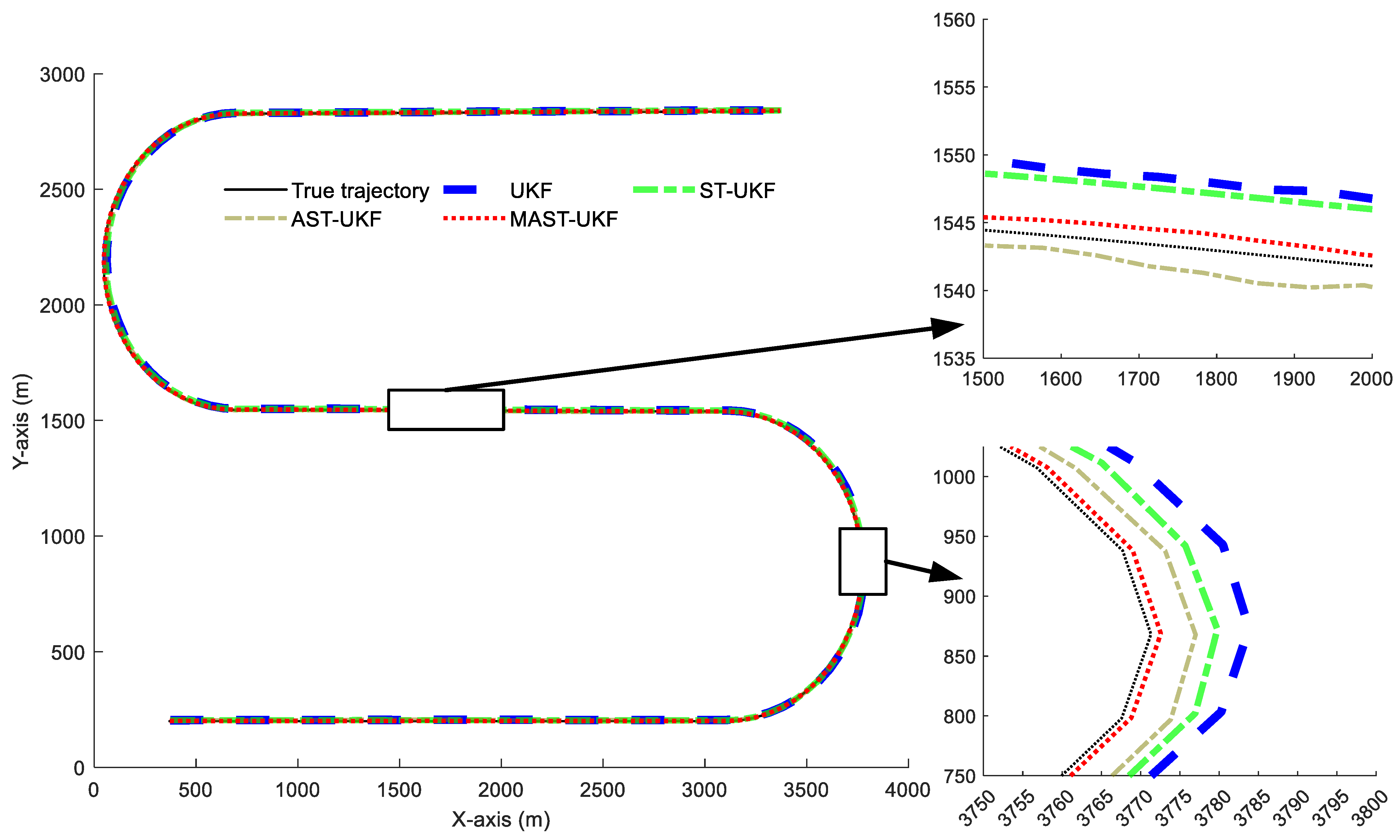
3.3. Simulation Experiments and Analysis

The simulation model measures the target using polar coordinates, and the measurement results are displayed on a bird’ s-eye view plane. During the simulation process, MATLAB 2022a, along with a laptop computer equipped with an Intel i9-12900H processor, Intel, Santa Clara, CA, USA and an NVIDIA RTX 3060 graphics card, Nvidia, Santa Clara, CA, USA, were used as the hardware and software platform to verify the performance of the designed algorithm for high-speed tracking of a moving target under wide-ranging maneuvering conditions.

To ensure the accuracy of the simulation, 200 Monte Carlo simulations were performed. The initial state of the target is set as $x_0={[300\mathrm{m},70\mathrm{m}/\mathrm{s},0{\mathrm{m}/\mathrm{s}}^2,200\mathrm{m}]}^T$, with the radar located at a fixed position relative to the target. The target’s initial position is $P_r={[x_0,y_0]}^T=[0,0]$. The observation period is $T=1\mathrm{s}$, with a total simulation time of 175 s. The simulation introduces Gaussian noise with a mean of zero. The measurement noise covariance matrix is given by $R_k=\mathrm{diag}\left([{50}^2,0.1^2]\right)$, and the measurement distance and angle errors are assumed to have biases of 50 m and 0.1°, respectively. We used three models, CV, CA, and CT models, each with an initial probability of ${\mu }_0={\left({\displaystyle \frac{1}{3}},{\displaystyle \frac{1}{3}},{\displaystyle \frac{1}{3}}\right)}^T$ and a Markov probability transfer matrix of P:

$$P=\left[\begin{array}{ccc}0.8& 0.1& 0.1\\ 0.1& 0.8& 0.1\\ 0.1& 0.1& 0.8\end{array}\right]$$

(25)

The target movement patterns are shown in

Table 1. Target motion model.

Time	Motion Model
0–40 s	(70 m/s, 0 m/s) CV motion
41–75 s	Constant Turn (CT) motion with angular velocity of 0.1 rad/s
76–100 s	Constant Acceleration (CA) motion with acceleration of (0.1 m/s², 0 m/s²)
101–135 s	Constant Turn (CT) motion with angular velocity of −0.1 rad/s
136–175 s	(70 m/s, 0 m/s) CV motion

.

In this simulation, we compared four algorithms, UKF [8], ST-UKF [9], AST-UKF [20], and MAST-UKF, to evaluate their tracking performance in complex traffic scenarios. UKF, as the benchmark method for nonlinear state estimation, was selected to verify the improvement of the adaptive mechanism on nonlinear tracking performance. ST-UKF and AST-UKF represent improved versions in terms of numerical stability and adaptive noise regulation, respectively. Compared with ST-UKF, the aim is to demonstrate that the multidimensional adaptive mechanism is more effective than the one-dimensional square-root improvement; compared with AST-UKF, it shows the superior generalization ability of multidimensional attenuation factors in handling complex motions (such as frequent switching between CV/CA/CT models). These comparisons enable the verification of the MAST-UKF’s tracking performance on moving targets at high speed and wide-range maneuvering conditions.

The experimental results are shown in Figure 2. It can be observed that the target’s motion state changed at the 41st second. First, during the turning process, MAST-UKF demonstrated the best tracking accuracy, followed by AST-UKF, ST-UKF, and finally, UKF. The specific reason is that MAST-UKF adjusts the state noise covariance by introducing multidimensional adaptive attenuation factors, which allows it to better adapt to inaccurate system state models and noise characteristics when the target state undergoes drastic changes, thereby improving tracking accuracy. In contrast, AST-UKF uses an adaptive attenuation factor with a strong tracking mechanism, which effectively adjusts the noise covariance. However, its ability to adapt to the system model during turning is slightly inferior to MAST-UKF, thus performing second best. ST-UKF improves accuracy by increasing the state noise covariance, and although it performs better than UKF, it still falls short of AST-UKF and MAST-UKF. The UKF algorithm has poor tracking accuracy during turning due to its fixed-noise covariance setting.

After entering the straight section, both MAST-UKF and AST-UKF maintained good tracking performance. The UKF algorithm, influenced by the previous CT motion, exhibited fluctuations in tracking performance. Similarly, ST-UKF showed poor tracking due to delays in adjusting the attenuation factor when the model changed.

Overall, during the entire tracking process, MAST-UKF and AST-UKF performed excellently, especially when the target state underwent drastic changes (such as turning). MAST-UKF, with the advantage of its multidimensional adaptive attenuation factors, provided the most stable and accurate tracking results. AST-UKF followed closely behind, performing well but not as flexibly as MAST-UKF in handling complex dynamic changes.

Table 2. RMSEs of different tracking algorithms.

Tracking Algorithm	X-Axis Position (m)	Y-Axis Position (m)	X-Axis Velocity (m/s)	Y-Axis Velocity (m/s)
UKF	2.3216	1.3404	1.2297	0.7064
ST-UKF	2.1833	1.2605	1.1925	0.6924
AST-UKF	2.0679	1.1939	1.1066	0.6396
MAST-UKF	1.7485	1.0057	0.7704	0.4456

compares the average errors of the five tracking algorithms. The results show that the MAST-UKF algorithm performs the best on both the X and Y axes of position and velocity, with the slightest error and the highest tracking accuracy; AST-UKF is the following best, while UKF has the most significant error and the worst performance. The tracking errors of MAST-UKF are reduced by 32.67%, 28.54%, and 23.17% compared to UKF, ST-UKF, and AST-UKF. Overall, the MAST-UKF algorithm significantly improves the tracking accuracy and outperforms the other algorithms.

Figure 3a shows the distance error comparison of the filtering algorithms, while Figure 3b shows the velocity error comparison. Based on the simulation results, the tracking performance of five algorithms was analyzed. Among these filtering algorithms, the MAST-UKF algorithm demonstrated the highest estimation accuracy, followed by the ST-UKF and AST-UKF algorithms with similar accuracy. In contrast, the UKF algorithm showed the lowest accuracy. In the simulation experiments, initial abnormal errors were not considered. When the target’s motion state underwent significant changes, the RMSE (root mean square error) of position and velocity increased in the other four filtering algorithms, and they failed to converge quickly. The main reasons for this were mismatched motion models and the impact of measurement outliers. In comparison to other filtering algorithms, MAST-UKF achieved the best estimation accuracy and error convergence when the target underwent large-scale maneuvers. The reason for this is that the MAST-UKF algorithm proposed in this study has strong adaptive adjustment capabilities, which effectively suppress the impact of measurement and motion model errors on estimation accuracy. As a result, the MAST-UKF algorithm demonstrates excellent error adaptive convergence performance when there are significant changes in the target’s motion state.

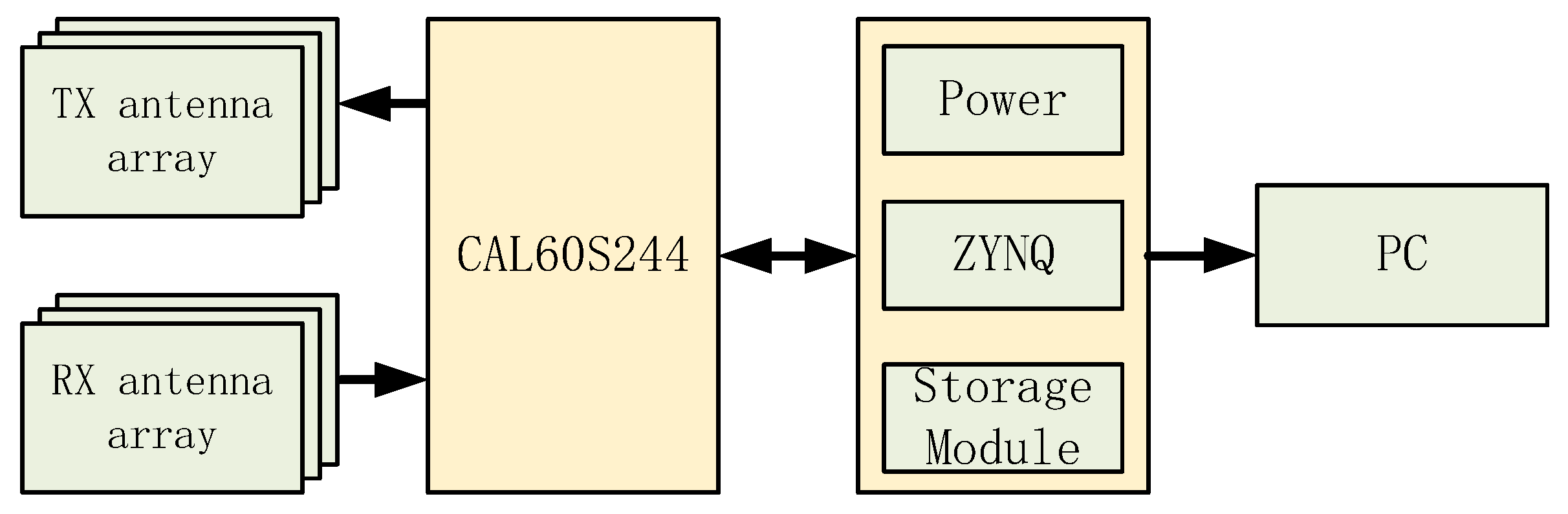
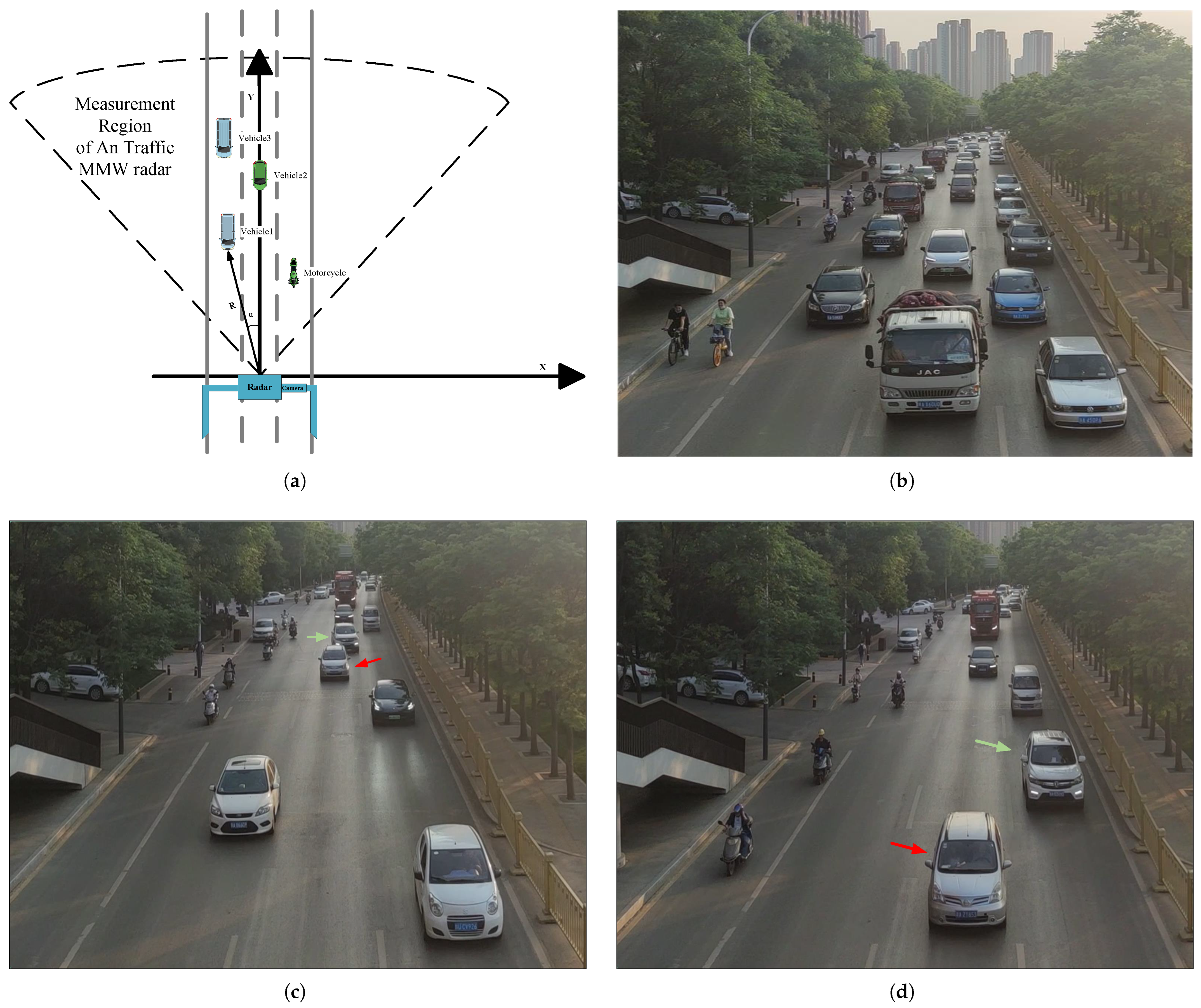
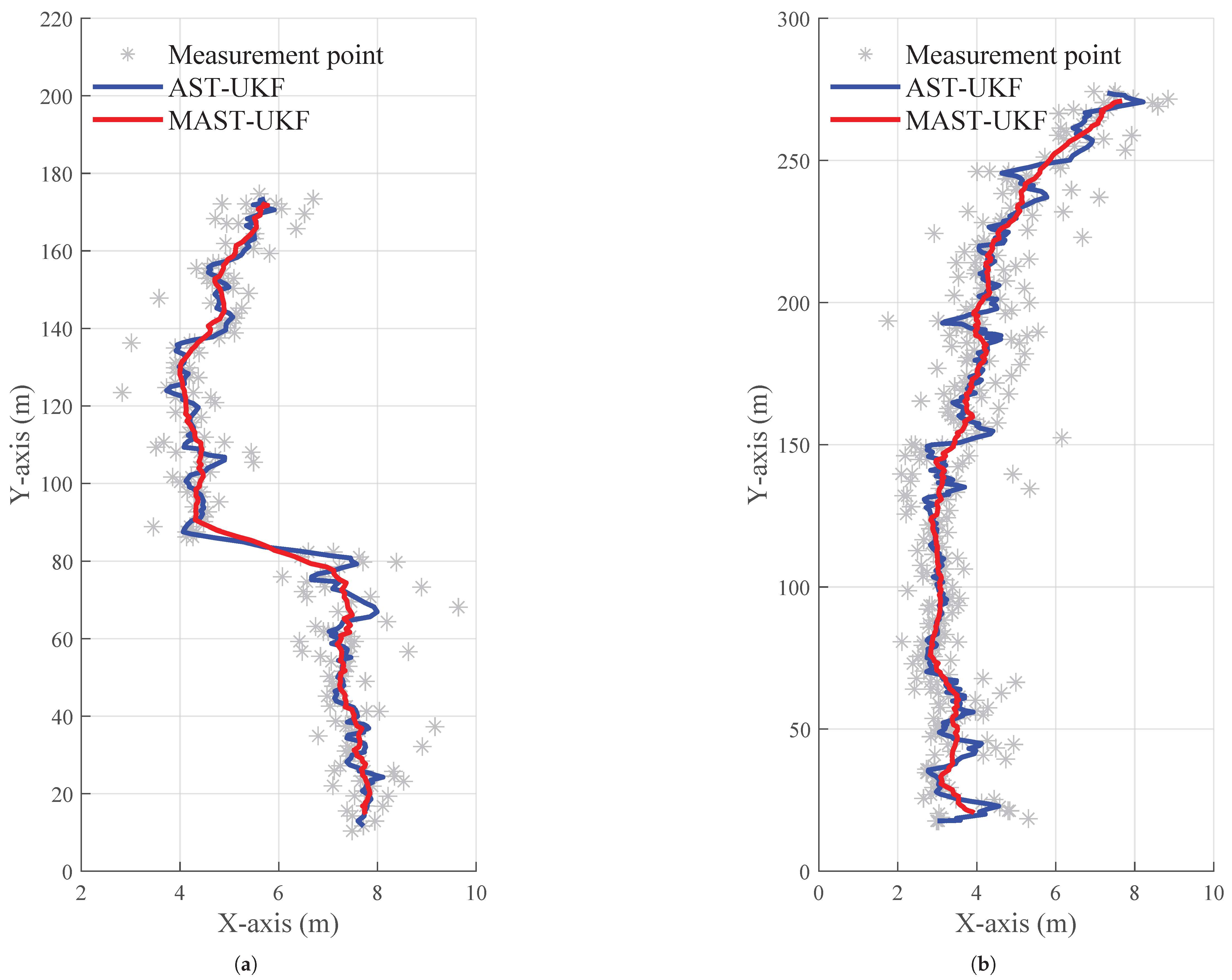
4. Real Experimental Results and Discussion

The measured data are entirely sourced from the data collection of a one-way, three-lane section of a road in Xi’an (the scene dataset is the same as in Reference [2]). The baseband signal processor is the ZYNQ-7020, produced by Xilinx, San Jose, CA, USA. The millimeter-wave radar RF chip is the CAL60S244 from Caltech, Pasadena, CA, USA. The hardware architecture of the millimeter-wave radar system is shown in Figure 4. The system is primarily composed of the RF board and the baseband board. The RF board includes the RF chip and the array transceiver antenna module, while the baseband board contains the power module, signal processing module, and storage module. The storage module is used to temporarily store data received by the radar or intermediate processing results, helping to avoid processing bottlenecks caused by data flow rates that exceed processing capacity.

The parameters of the radar setup are shown in

Table 3. Radar system parameters and performance indicators.

Radar System Parameters	Parameter Value	Unit
Operating Frequency Range	60–61	GHz
Number of TX/RX Antenna Array	4T/4R	-
Signal Bandwidth	200	MHz
Signal Pulse Period	30	μs
Tuning Frequency Rate	6.7	MHz/μs
Distance Resolution	0.75	m
Speed Resolution	0.1	m/s
Angle Resolution	0.1	°
Data Rate	20	Hz

.

Before the radar installation, angle calibration and testing are required to ensure the accuracy of the millimeter-wave radar (MMW) measurements. An angle controller, lane markings, and corner reflectors are used for calibration. The standard measurement error of the radar is ±0.03 m/s. As shown in Figure 5a, the traffic millimeter-wave radar detection system uses angular calibration to ensure the radar antenna is parallel to the lane direction. After the radar antenna calibration is completed, the radar equipment is installed on an overpass beside the road as a fixed observation point. Figure 5b illustrates the actual deployment of the radar system. Data collection is conducted through a host computer that is connected to the radar system in real time. The host computer receives, processes, and stores the measurement data, such as vehicle speed and position, collected by the millimeter-wave radar.

Figure 6a shows the relationship between the traffic millimeter-wave radar, the camera, and the target. During the data collection process, synchronized data acquisition was performed using both the motion camera and the millimeter-wave radar. The camera and radar were installed on two separate mounts and placed close to each other to ensure they covered the same observation area. Figure 6b illustrates a complex traffic scenario with heavy traffic flow and closely matched vehicle speeds. During the experiment, to evaluate the effectiveness of the MAST-UKF algorithm, data from two vehicles were compared: Vehicle A changes lanes during its movement, while Vehicle B simultaneously continues to drive straight. Vehicle A starts being tracked at the 27th second, with continuous tracking from frame 632 to frame 918. Vehicle B starts being tracked at the 24th second, with the tracking interval from frame 573 to frame 929. Figure 6c,d show the images of the two target vehicles.

The tracking results of the MAST-UKF algorithm are shown in Figure 7a,b. An analysis of the measurement data, filtered tracking data, and recorded video indicate that the system is capable of reliably tracking the experimental vehicles. Moreover, after post-filtering, the vehicle’s tracking trajectory becomes more consistent, with minimal deviation, even in the presence of measurement outliers. The filtered trajectory of the target vehicle matches its actual motion state during lane changes, with the velocity filter values converging without divergence.

The MAST-UKF algorithm tracks target vehicles A and B. The actual vehicle experimental results provide the root mean square error (RMSE) of the absolute position of the vehicles in the Cartesian coordinate system, as shown in

Table 4. Table of average distance errors for different tracking algorithms.

Tracking Algorithm	A X-Axis Position (m)	A Y-Axis Position (m)	B X-Axis Position (m)	B Y-Axis Position (m)
AST-UKF	0.1705	0.7218	0.1039	0.7052
MAST-UKF	0.1568	0.4892	0.0971	0.5193

, and the root mean square error of the absolute velocit (

Table 5. Table of average velocity errors for different tracking algorithms.

Tracking Algorithm	A X-Axis Position (m)	A Y-Axis Position (m)	B X-Axis Position (m)	B Y-Axis Position (m)
AST-UKF	0.1970	1.2894	0.1638	1.1379
MAST-UKF	0.1836	0.9372	0.1547	0.8836

). Compared to the AST-UKF algorithm, the distance error is reduced by 18.29%, and the velocity error is reduced by 15.25%.

In addition, we also tested the operating speed of AST-UKF and MAST-UKF to evaluate their performance in actual system operations. This experiment was conducted in five rounds, comparing the two algorithms by continuously running them 1000 times on the computer. The time required for the continuous running of AST-UKF and MAST-UKF algorithms was recorded. The experimental results are shown in

Table 6. Computational time for different algorithms.

Rounds	AST-UKF	MAST-UKF
1	44.222 s	48.285 s
2	43.572 s	48.398 s
3	44.171 s	48.438 s
4	43.865 s	48.438 s
5	43.686 s	47.876 s

.

It can be seen that the execution speed of MAST-UKF is slower than AST-UKF, with the time for 1000 iterations being 47.876 s, while AST-UKF took 48.444 s. The results show that the algorithm requires slightly more time for calculation. However, it is noteworthy that the average running time of MAST-UKF meets the practical processing requirements, reaching the lowest demand of 50 milliseconds per iteration. The table also shows that MAST-UKF, while slower than AST-UKF, has more practical efficiency and supports real-world applications, especially in dynamic environments that require high-efficiency target tracking and data processing.

In summary, the MAST-UKF algorithm proposed in this paper can adaptively adjust the noise covariance using the improved attenuation factor. It achieves good tracking of large-range maneuvering targets when their motion state undergoes significant changes while ensuring real-time performance.

5. Conclusions

In this paper, we propose a Strong Tracking Unscented Kalman Filter algorithm based on multidimensional adaptive attenuation factors (MAST-UKF). To address the issue of decreased tracking accuracy in the traditional Strong Tracking Unscented Kalman Filter algorithm when the target’s motion state undergoes significant changes, we introduced a multidimensional adaptive attenuation factor diagonal matrix before the state noise covariance and observation noise covariance to perform adaptive adjustment. The experimental results show that the MAST-UKF algorithm can effectively improve the tracking performance of targets under complex conditions by adjusting the noise covariance through the adaptive factor.

However, due to the relatively slow adjustment of the state noise covariance by the adaptive factor introduced by MAST-UKF and the overall high computational complexity, the algorithm’s convergence is somewhat limited. To further improve the algorithm’s adaptability and efficiency, future research could consider optimizing the attenuation factor adjustment strategy using methods such as reinforcement learning or applying hardware acceleration techniques (such as GPU acceleration and parallel processing) to enhance filtering efficiency. Additionally, this paper only uses millimeter-wave radar (MMW Radar) for target tracking, which limits the system’s application in multi-sensor fusion. Future studies could combine MAST-UKF with other sensors, such as LiDAR, cameras, and Global Navigation Satellite Systems (GNSSs), to further reduce the errors of single sensors and improve the system’s accuracy and robustness.

References

1. Huang, K.; Ding, J.; Deng, W. An Overview of Millimeter-Wave Radar Modeling Methods for Autonomous Driving Simulation Applications. Sensors 2024, 24, 3310. [Google Scholar] [CrossRef] [PubMed]
2. Tian, F.; Guo, X.; Fu, W. Target Tracking Algorithm Based on Adaptive Strong Tracking Extended Kalman Filter. Electronics 2024, 13, 652. [Google Scholar] [CrossRef]
3. Wu, G.; Zhou, F.; Meng, C.; Li, X.Y. Precise UAV MMW-Vision Positioning: A Modal-Oriented Self-Tuning Fusion Framework. IEEE J. Sel. Areas Commun. 2023, 42, 6–20. [Google Scholar] [CrossRef]
4. Liu, Z.; Chen, Y.; Lu, Y. Mid-state Kalman filter for nonlinear problems. Sensors 2022, 22, 1302. [Google Scholar] [CrossRef] [PubMed]
5. Zong, M.; Zhu, Z.; Wang, H. A simulation method for millimeter-wave radar sensing in traffic intersection based on bidirectional analytical ray-tracing algorithm. IEEE Sens. J. 2023, 23, 14276–14284. [Google Scholar] [CrossRef]
6. Liang, L.; Ma, H.; Zhao, L.; Xie, X.; Hua, C.; Zhang, M.; Zhang, Y. Vehicle detection algorithms for autonomous driving: A review. Sensors 2024, 24, 3088. [Google Scholar] [CrossRef] [PubMed]
7. Chen, K.; Shao, J.; Zhang, Y.; Liu, K. A Target-based co-calibration framework for 3DRadar-camera using a modified corner reflector. Meas. Sci. Technol. 2024, 35, 047002. [Google Scholar] [CrossRef]
8. Julier, S.J.; Uhlmann, J.K. Unscented filtering and nonlinear estimation. Proc. IEEE 2004, 92, 401–422. [Google Scholar] [CrossRef]
9. Wang, X.X.; Zhao, L.; Xia, Q.X.; Hao, Y. Strong tracking filter based on unscented transformation. Control Decis. 2010, 25, 1063–1068. [Google Scholar]
10. Li, P.; Zhou, G. Target Tracking With Revisit Interval Uncertainty for Rotating Radars. IEEE Trans. Aerosp. Electron. Syst. 2024, 60, 7354–7366. [Google Scholar] [CrossRef]
11. Dahal, P.; Mentasti, S.; Arrigoni, S.; Braghin, F.; Matteucci, M.; Cheli, F. Extended object tracking in curvilinear road coordinates for autonomous driving. IEEE Trans. Intell. Veh. 2022, 8, 1266–1278. [Google Scholar] [CrossRef]
12. Elsergany, A.M.; Abdel-Hafez, M.F.; Jaradat, M.A. Novel augmented quaternion UKF for enhanced loosely coupled GPS/INS integration. IEEE Trans. Control Syst. Technol. 2024, 32, 2321–2331. [Google Scholar] [CrossRef]
13. Sun, W.; Zhao, J.; Ding, W.; Sun, P. Robust UKF relative positioning approach for tightly coupled vehicle ad hoc networks based on adaptive M-estimation. IEEE Sens. J. 2023, 23, 9959–9971. [Google Scholar] [CrossRef]
14. Wang, P.; Liu, C.; Zhang, J.; Wang, L.; Zhang, M. DS-UKF-Based Positioning Method for Intelligent Connected Vehicles in Urban Intersection Scenarios. IEEE Trans. Intell. Transp. Syst. 2023, 25, 6118–6132. [Google Scholar] [CrossRef]
15. Yang, Y.; Wang, X.; Zhang, N.; Gao, Z.; Li, Y. Artificial neural network based on strong track and square root UKF for INS/GNSS intelligence integrated system during GPS outage. Sci. Rep. 2024, 14, 13905. [Google Scholar] [CrossRef] [PubMed]
16. Yuan, S.; Wu, J.; Luan, F.; Zhang, L.; Lv, J. Improvement of Strong Tracking UKF-SLAM Approach using Three-position Ultrasonic Detection. Robot. Auton. Syst. 2023, 159, 104305. [Google Scholar] [CrossRef]
17. Zhao, G.; Jiang, Z.; Wang, J.; Gao, S. A robust SVD-UKF algorithm and its application in integrated navigation systems. Adv. Space Res. 2025, 75, 1902–1912. [Google Scholar] [CrossRef]
18. Zhang, X.; Yuan, S.; Yin, X.; Li, X.; Qu, X.; Liu, Q. Estimation of skid-steered wheeled vehicle states using STUKF with adaptive noise adjustment. Appl. Sci. 2021, 11, 10391. [Google Scholar] [CrossRef]
19. Tian, F.; Wang, J.; Li, K. A Novel Strong Tracking ETUKF for State Estimation of Preceding Vehicles Using V2V Communications. IEEE Trans. Veh. Technol. 2023, 72, 12500–12507. [Google Scholar] [CrossRef]
20. Huang, P.; Li, H.; Wen, G.; Wang, Z. Application of adaptive weighted strong tracking unscented kalman filter in non-cooperative maneuvering target tracking. Aerospace 2022, 9, 468. [Google Scholar] [CrossRef]
21. Zhang, W.; Hou, Y. A Modified Strong Tracking Adaptive Kalman Filter for Precision Clock Synchronization System. Ieej Trans. Electr. Electron. Eng. 2023, 18, 1702–1711. [Google Scholar] [CrossRef]
22. Liu, J.; Chen, X.; Wang, J. Strong tracking UKF-based hybrid algorithm and its application to initial alignment of rotating SINS with large misalignment angles. IEEE Trans. Ind. Electron. 2022, 70, 8334–8343. [Google Scholar] [CrossRef]
23. Yan, X.; Zhao, L.; Tang, C.; Zou, J.; Gao, W.; Jian, J.; Jin, Q.; Zhang, X. Intelligent MEMS Thermal Mass Flowmeter Based on Modified Sage-Husa Adaptive Robust-Strong Tracking Kalman Filtering. IEEE Sens. J. 2024, 25, 283–290. [Google Scholar] [CrossRef]
24. Yang, Y.; Ding, J.; Shen, D.; Hao, T. Optimal Informat20es. J. Electrochem. Soc. 2023, 170, 090528. [Google Scholar] [CrossRef]
25. Zhao, J.; Zhang, Y.; Li, S.; Wang, J.; Fang, L.; Ning, L.; Feng, J.; Zhang, J. An Improved Unscented Kalman Filter Applied to Positioning and Navigation of Autonomous Underwater Vehicles. Sensors 2025, 25, 551. [Google Scholar] [CrossRef]
26. Zhao, J.; Wang, M.; Hu, X.; Zhang, L. Precise Pre-Close Wind Volume Calculation for Aluminum Electrolysis Based on Unscented Kalman and Average Filters. Appl. Sci. 2024, 14, 12046. [Google Scholar] [CrossRef]
27. Zhou, Z.; Zhan, M.; Wu, B.; Xu, G.; Zhang, X.; Cheng, J.; Gao, M. A novel adaptive unscented kalman filter algorithm for SOC estimation to reduce the sensitivity of attenuation coefficient. Energy 2024, 307, 132598. [Google Scholar] [CrossRef]
28. Singh, H.; Mishra, K.V.; Chattopadhyay, A. Inverse Unscented Kalman Filter. IEEE Trans. Signal Process. 2024, 72, 2692–2709. [Google Scholar] [CrossRef]
Figure 1. The flowchart of the MAST-UKF algorithm.
Applsci 15 03276 g001
Figure 2. Tracking results for each filtering algorithm.
Applsci 15 03276 g002
Figure 3. Filter tracking error plot. (a) RMSE of position; (b) RMSE of velocity.
Applsci 15 03276 g003
Figure 4. Radar hardware system architecture.
Applsci 15 03276 g004
Figure 5. Traffic MMW radar detection system implementation. (a) Calibration of traffic MMW radar; (b) measurement data acquisition.
Applsci 15 03276 g005
Figure 6. Schematic of the experimental scenario and objectives: (a) geometric relationship diagram between the traffic MMW radar and the target object; (b) traffic scenario during a complex traffic peak period; (c) image of the tracked target vehicle at frame 798; and (d) image of the tracked target vehicle at frame 916.
Applsci 15 03276 g006
Figure 7. Tracking results: (a) objective A; (b) objective B.
Applsci 15 03276 g007