A Prediction-Based Anomaly Detection Method for Traffic Flow Data with Multi-Domain Feature Extraction

Abstract

The core idea of prediction-based anomaly detection is to identify anomalies by constructing a prediction model and comparing predicted and observed values. However, most existing traffic flow prediction models primarily focus on spatio-temporal features, neglecting comprehensive frequency-domain feature learning. Additionally, anomaly detection accuracy is often limited by insufficient prediction error analysis. To address this limitation, this paper proposes a prediction-based anomaly detection method for traffic flow data with multi-domain feature extraction. The prediction model is built as follows: first, Bidirectional Long Short-Term Memory network (Bi-LSTM) and a Graph Attention Network (GAT) extract temporal and spatial features, respectively. Then, Fast Fourier Transform (FFT) converts time-domain signals into the frequency domain, where Transformer learns magnitude and phase features. Finally, a prediction model is constructed using the extracted time-domain and frequency-domain features. For error analysis, this paper innovatively applies Chebyshev’s inequality to determine the error threshold, identifying anomalies based on whether errors exceed this threshold. Experimental results show that integrating multi-domain features can more comprehensively capture data characteristics and improve model prediction accuracy. In the anomaly detection experiment, it was verified that constructing a high-accuracy prediction model and conducting reasonable error analysis can effectively enable anomaly detection in the data.

1. Introduction

Time series data refers to a collection of data points associated with specific time components, typically recorded at uniform time intervals [1]. This type of data reflects the state or magnitude of a particular phenomenon or object over time [2].

Multivariate Time Series (MTS) is a set of time series that share the same timestamps. At each time point, data is represented as an array of variables or numerical values, essentially forming a collection of multiple univariate time series captured over time [1]. This data structure enables the analysis of relationships and dynamic changes among variables, serving as a crucial tool for studying complex systems and exploring interactions across various domains. In the evolving field of time series analysis, identifying patterns and dynamic changes is essential for accurate forecasting and deep insights [3].

Traffic flow data is a typical example of MTS, exhibiting complex temporal characteristics such as long-term trends, seasonality, periodicity, and randomness. For instance, commuting traffic increases during morning and evening rush hours but drops significantly at night; commercial areas may be busier on weekends, while commuter routes experience lower traffic; highway traffic surges during long holidays, whereas urban road traffic decreases; sudden accidents can cause a sharp drop in traffic, followed by a congestion recovery phase.

Additionally, the propagation of traffic flow within a road network is constrained by its topology. Traffic flow is not independently distributed but is influenced by upstream and downstream road segments. There is often a strong correlation between adjacent road segments or regions. Thus, beyond the typical characteristics of MTS data, traffic flow also exhibits complex spatial features.

While analyzing data characteristics, it is essential to consider not only its temporal and spatial properties but also its frequency-domain features. For example, in traffic flow data, the magnitude of different frequency components after time-frequency transformation represents the signal’s energy at various frequencies, while the frequency corresponding to the maximum magnitude indicates the primary traffic cycle. In signal processing and time series analysis, time-domain and frequency-domain methods each have their strengths and limitations. Combining both approaches leverages their complementary advantages, enhancing signal analysis and feature extraction. This integration enables a more comprehensive examination of signals across both time and frequency dimensions, overcoming the limitations of a single analysis method.

Anomalies in traffic flow data often indicate special situations, such as equipment failures or unexpected incidents within specific time periods. Failure to detect these anomalies in a timely and accurate manner may lead to severe consequences. Fast and effective anomaly detection helps identify potential issues early, minimizing unnecessary economic losses [4]. Therefore, efficiently extracting potential anomalies from data holds significant practical value.

However, specialized anomaly detection methods for traffic flow data remain scarce. Existing studies often adopt a uniform detection approach without fully considering the varying needs of different domains. Moreover, many methods primarily focus on the spatio-temporal characteristics of traffic flow data while overlooking its frequency-domain features, limiting the exploration of periodic patterns. This single-dimensional analysis lacks specificity in handling traffic anomalies, making it challenging to accurately capture complex abnormal patterns.

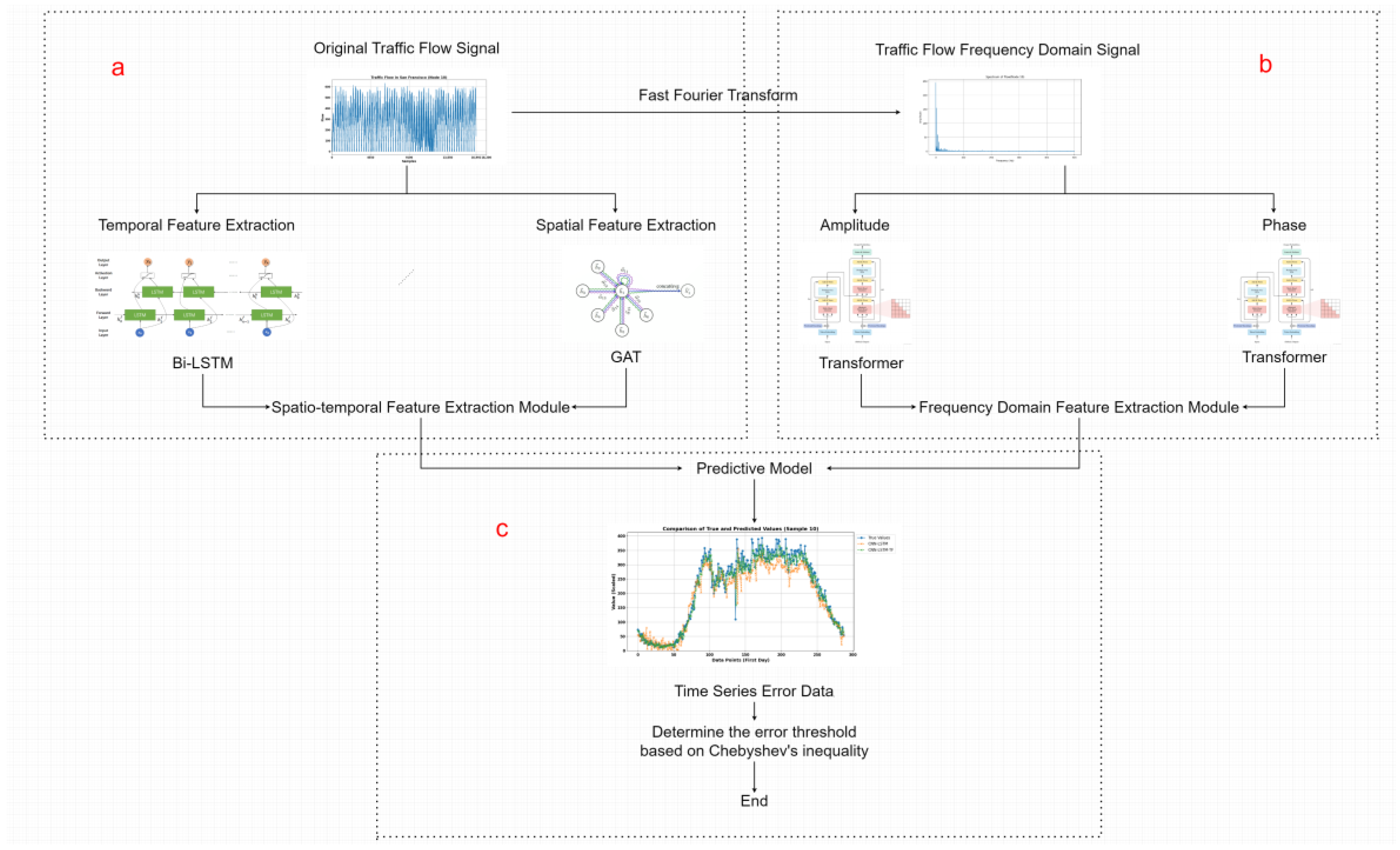
To achieve more precise anomaly detection in traffic flow data, this paper proposes a prediction-based anomaly detection method for traffic flow data with multi-domain feature extraction. The key innovations of this method are as follows:

• Optimizing the Prediction Model by Combining Data Characteristics

This method not only focuses on the temporal characteristics of traffic flow data but also fully considers the spatial correlations between the data. By using different models to jointly learn both temporal and spatial features, it enables feature extraction in the time domain. Additionally, recognizing that traffic flow data often exhibits periodicity and may be subject to noise interference, this paper leverages the advantages of frequency-domain analysis (such as periodicity identification and noise suppression) to further explore the frequency-domain characteristics of the data. The model then learns its frequency-domain representation, achieving more comprehensive feature extraction. Experimental results show that prediction models that fully explore data features can significantly improve prediction accuracy.

2.

Error Analysis and Threshold Determination

Prediction-based methods are widely used in anomaly detection, relying on the difference between predicted and observed values to identify anomalies. However, determining an appropriate error threshold in existing methods often lacks adaptability and reliability. To address this issue, this paper introduces Chebyshev’s inequality to establish a more scientific and rational threshold for error analysis, thereby enhancing the accuracy and robustness of anomaly detection.

2. Related Work

In real-world monitoring scenarios, traffic flow data collected by sensors is typically unlabeled [5] and often suffers from incompleteness due to various objective factors, leading to anomalies and missing data. This necessitates anomaly detection models with unsupervised learning capabilities [6,7]. Additionally, the high dimensionality, dynamic nature, and complexity of MTS data [8] make accurately identifying anomalous data a challenging task.

Currently, unsupervised time series anomaly detection methods can be broadly categorized into traditional and deep learning-based approaches. Common traditional methods include statistical approaches (both parametric and non-parametric) as well as reconstruction and clustering techniques based on classical machine learning. In contrast, deep learning-based methods primarily focus on prediction and reconstruction. Statistical methods typically model each variable in MTS data independently, failing to fully leverage the spatial relationships among multiple variables. For highly correlated MTS data, anomaly detection methods based on classical machine learning and deep learning have become the dominant trend in research and application.

Reconstruction-based anomaly detection methods for multivariate time series involve training models to learn latent representations of normal time subsequences, reconstructing the multivariate subsequences, and identifying anomalies by measuring the differences between the reconstructed and original sequences. Principal Component Analysis (PCA) is a classical dimensionality reduction and feature extraction technique [9]. It detects anomalies by assessing whether a data sample can be effectively reconstructed. If a sample is difficult to reconstruct, its features are likely inconsistent with the overall dataset, indicating it as an anomaly. Aosong et al. [10] applied an improved PCA-based method to detect faults in chiller sensors. Qu et al. [11] proposed an optimization approach that minimizes intra-class reconstruction errors while maximizing inter-class reconstruction errors for training samples. Rashidi et al. [12] introduced a standardized reconstruction error metric, providing a more effective means for accuracy evaluation. Ana et al. [13] adopted a partially interpretable autoencoder structure to enhance PCA’s data compression and reconstruction capabilities. Dan et al. [14] developed a novel semi-supervised anomaly detection framework based on reconstruction similarity. Ji et al. [15] proposed a new anomaly detection framework that integrates statistical analysis with neural network methods.

Clustering-based anomaly detection is a typical unsupervised method that distinguishes anomalies based on three common assumptions: data points that do not belong to any cluster are anomalies, data points far from the cluster centers are anomalies, and data points within sparse or small clusters are anomalies. Aziz et al. [16] applied K-means clustering to Call Detail Records (CDRs) from both anomaly detection and prediction perspectives, proposing a scalable and efficient anomaly detection method. Rajeshkumar et al. [17] optimized anomaly detection models by enhancing machine learning classifiers. Wang et al. [18] introduced an anomaly detection algorithm combining clustering techniques with autoencoder models to identify network traffic anomalies.

With the widespread application potential of deep learning across various fields, deep learning-based time series anomaly detection methods have garnered significant attention. These methods can learn complex nonlinear temporal relationships and high-dimensional representations of time series data. Nallappan et al. [19] proposed a content-based video retrieval (CBVR) framework for anomaly detection in surveillance videos, leveraging deep learning techniques and HNSW (Hierarchical Navigable Small World) indexing. Iqbal et al. [20] applied various deep learning models for anomaly detection and time series forecasting and introduced a statistical method to overcome the limitations of high-dimensional time series data. Shafeiy et al. [21] introduced the pioneering MCN-LSTM technique for real-time water quality monitoring, addressing the challenges of detecting anomalies in complex time series data.

With the continuous optimization of forecasting models and methods, prediction-based anomaly detection techniques have shown significant development potential. Changzhi et al. [22] applied forecasting methods to detect anomalies in power data. Takahashi et al. [23] proposed using seasonal thresholds to improve prediction-based detection methods, addressing the challenge of determining error thresholds.

Table 1. Comparison of Various Anomaly Detection Methods.

Applied Method	Advantages	Disadvantages
PCA and Improved PCA Methods	Achieves simple fault detection by replicating and enhancing PCA’s data compression and reconstruction capabilities.	Limited by PCA’s linear nature, making it challenging to handle complex nonlinear relationships; computationally intensive.
Refactoring-based methods and improved refactoring methods	Provides a more effective accuracy assessment method, improving the precision of anomaly detection.	This approach offers a more effective means of accuracy assessment, enhancing the precision of anomaly detection.
Clustering Algorithms and Improved Clustering Algorithms	Scalable and efficient methods for anomaly detection.	Sensitive to the choice of hyperparameters; requires a large amount of normal data for training, potentially limiting the ability to detect novel anomalies.
Prediction-Based Anomaly Detection Methods	Capable of learning more complex nonlinear temporal relationships and representations of high-dimensional time series.	Prediction errors can impact detection performance; may lack adequate error analysis.
Seasonal Threshold + Prediction Methods	Improves the determination of error thresholds.	Assumptions about seasonality may not apply to all time series data.

presents a comparison of various anomaly detection methods.

With the further advancement of deep learning, predictive models now consider not only the temporal dependencies of samples but also the spatial dependencies, including the network topology of the samples. Kidu et al. [24] extracted spatio-temporal features from samples to predict and identify driver activities. Ullah et al. [25] proposed a one-dimensional hybrid CNN-LSTM method to extract spatio-temporal features for detecting pipeline leaks. Tipper et al. [26] used CNN and LSTM for deepfake video detection. Xiong et al. [27] introduced a data-augmented SSA-CNN-LSTM framework for fault prediction. Li et al. [28] introduced a multi-feature extraction neural network model based on Convolutional LSTM for predicting PM2.5 levels in air quality forecasting, achieving effective integration of spatial correlations. Jiawei et al. [29] proposed a novel detection method based on CNN and LSTM networks to comprehensively explore spatio-temporal information.

In the time domain, the focus is typically on the transient characteristics of a signal, which reflect how the signal changes over time and are suitable for monitoring dynamic variations. In contrast, in the frequency domain, complex time-domain signals are decomposed into components of different frequencies. Analyzing these frequencies effectively identifies and suppresses noise, with an emphasis on the periodic characteristics of the signal. Frequency domain analysis is a method that examines the characteristics of a signal in the frequency domain. Pascale et al. [30] revealed the differences in the contribution of frequency components to the overall signal at different speeds through the analysis of noise emissions from two distinct motorized sources. Li et al. [31] proposed a Global Navigation Satellite System (GNSS) spoofing detection method based on frequency domain processing. Combining time domain and frequency domain characteristics provides a more comprehensive perspective, improving the efficiency and accuracy of feature extraction and facilitating a better understanding and analysis of signal characteristics.

Predictive anomaly detection methods typically require the construction of an accurate forecasting model. By comparing the difference between predicted and observed values against a predefined threshold, anomalies can be identified. Based on the literature review, the following key challenges exist in the field of traffic flow anomaly detection:

• Lack of specialized anomaly detection methods for traffic flow data

While traffic flow data share typical characteristics of MTS data, they also exhibit strong spatial dependencies. However, existing methods often fail to account for these spatial properties.

2.

Limited consideration of frequency-domain features

Current predictive models primarily focus on time-domain methods, leveraging only temporal and spatial characteristics while overlooking frequency-domain properties. As a result, the feature learning process for MTS data remains incomplete.

3.

Uncertainty in error threshold determination

In predictive anomaly detection, setting an appropriate error threshold is challenging. Since error analysis is a crucial step in ensuring detection accuracy, the lack of a reliable threshold selection method can significantly impact the effectiveness of anomaly detection.

Based on the above issues and situation analysis, this paper proposes a prediction-based anomaly detection method for traffic flow data that incorporates multi-domain feature extraction. This method leverages both time-domain and frequency-domain features to comprehensively capture the temporal and spectral characteristics of the data, enabling the construction of an effective time series prediction model. By analyzing the predicted and observed values, the error threshold is determined using Chebyshev’s inequality, and anomalies are detected by checking whether the error falls within the threshold range. This approach enables effective detection of anomalous data points.

3. Methodology

3.1. Description of Anomaly Detection Methods

The anomaly detection method for traffic flow data based on prediction and multi-domain feature extraction proposed in this paper consists of two main parts: the construction of the prediction model and error analysis for anomaly detection. The overall framework is shown in Figure 1.

The construction of the prediction model primarily consists of two modules: the time-domain feature extraction module and the frequency-domain feature extraction module. The time-domain feature extraction module uses a Bidirectional Long Short-Term Memory network (Bi-LSTM) to capture the temporal dependencies in the data and a Graph Attention Network (GAT) to extract spatial dependencies, enabling the learning of both temporal and spatial characteristics in the time domain. The frequency-domain feature extraction module first applies Fast Fourier Transform (FFT) to convert the raw time-domain signal into a frequency-domain signal. Then, a Transformer model is used to separately extract the amplitude and phase features in the frequency domain, facilitating the learning of frequency-domain characteristics. The prediction model is constructed by integrating the features extracted from both the time and frequency domains.

In this paper, the traffic flow $X=\{x^1,x^2,x^3,\dots x^t\dots ,x^N\}\in R^{M\times N}$ is taken as an input, where $x^t=\{x_1^t,x_2^t,x_3^t,\dots ,x_M^t\}\in R^M$ is denoted as the observation measured at time $t=\{1,2,\cdots N\}$. The prediction model predicts the traffic flow for the time interval H at each node based on the observations in a historical time window K at that node, so the problem of traffic flow prediction at a particular node can be formulated as follows: $[x^{t_0-K+1},x^{t_0-K+2},\dots x^{t_0}]\stackrel{F}{\to }[{\widehat{x}}^{t_0+1},{\widehat{x}}^{t_0+2},\dots {\widehat{x}}^{t_0+H}]$,where F is the prediction model.

The error analysis and anomaly detection section uses Chebyshev’s inequality to determine the threshold value of error $e_i$, and analyzes whether the error $e_t$ between the observed value $x^t$ at a point in time $t$ and the predicted value ${\widehat{x}}^t$ at that point is within the threshold value to detect whether the data at that point is anomalous or not.

3.2. Time Domain Feature Extraction Module

3.2.1. Time Feature Extraction Based on Bi-LSTM

Long Short-Term Memory (LSTM) networks improve upon the Recurrent Neural Network (RNN) model by addressing issues such as gradient explosion and vanishing gradients, and they perform exceptionally well in sequence prediction tasks. Bi-LSTM is a bidirectional LSTM model that adds a backward layer to enable bidirectional reading. It consists of two LSTM models: a forward model and a backward model. The forward model processes the input sequence in the forward direction, from start to end, utilizing past information, while the backward model processes the sequence in reverse, from end to start, leveraging future information.

Traffic flow data exhibits typical time series characteristics. Bi-LSTM, at each time step, allows each LSTM unit to access both past and future contextual information, making it highly effective at capturing long-term dependencies in time series data.

The two LSTMs in Bi-LSTM have the same structure, and in the case of forward LSTM, for example, each time point LSTM in the input $X=\{x^1,x^2,x^3,\dots x^t\dots ,x^N\}$ combines the current input and the hidden state $\overrightarrow{h_{t-1}}$ of the previous time point to compute the output $O_t$. At the same time, the hidden state $\overrightarrow{h_t}$ of the current time point is used again as the input of the next time point, i.e.:

$$O_t=\sigma (W_0\cdot [h_{t-1},x^t]+b_0)$$

(1)

$$\overrightarrow{h_t}=O_t\cdot \mathit{tanh}(C_t)$$

(2)

where: $W_0$ and $b_0$ are the weights and biases, respectively; $\sigma$ is the activation function; $C_t$ denotes the state parameters at the current moment; tanh is the hyperbolic tangent activation function.

After the input goes through the LSTM, the output $X^T\in R^{h\times T}$ is obtained, where h is the dimension of the hidden layer of the LSTM. $X^T$ preserves the hidden state information at each time step and is a feature representation containing the temporal correlation of the data. Bi-LSTM, on the other hand, combines the forward and reverse LSTMs, and splices the hidden state $\overrightarrow{h_t}$ of the forward LSTM with the hidden state $\overleftarrow{h_t}$ of the reverse LSTM to obtain the Bi-LSTM output. LSTM output $h_t$, i.e.:

$$h_t=\sigma (W\cdot [\overrightarrow{h_t};\overline{\overleftarrow{h_t}}]+c).$$

(3)

3.2.2. Spatial Feature Extraction Based on GAT

Traffic flow data not only exhibits temporal features but also contains spatial relationships between the data points. While traditional time series models focus on extracting temporal features, modeling the spatial dependencies using network structures and attribute information is also crucial. A graph is composed of nodes and edges, and $G=\{V,E,A\}$ is used to define a transportation network. In this context, V represents the set of nodes, which corresponds to the collection of sensors in the highway system; E represents the set of edges, indicating the relationships between the nodes, or the connections between pairs of sensors; and A denotes the network’s adjacency matrix, typically a distance-weighted adjacency matrix that represents the connectivity between each node in the road network. By constructing this adjacency matrix, the original data can be transformed into graph data that captures spatial features.

In this paper, nodes with a connection are assigned a value of 1, while nodes without a connection are assigned a value of 0, constructing an adjacency matrix that transforms the raw data into graph data $A_{ij}$ with spatial correlations. During the spatial feature extraction process, $A_{ij}$ is used as input to learn the correlations between sensors, capturing the spatial relationships within the time series. Traffic conditions can be measured by H sensors, and the adjacency matrix can represent the relationships between different traffic states. This can be specifically expressed as the following matrix:

$$X_{\left(z,t\right)}={\left[\begin{array}{c}{X}_{\left(z,t_0-T+1\right)}\\ X_{\left(z,t_0-T+2\right)}\\ ⋮\\ X_{\left(z,t_0-1\right)}\\ X_{\left(z,t_0\right)}\end{array}\right]}^T=\left[\begin{array}{ccccc}{x}_{\left(z_1,t_0-T+1\right)}& x_{\left(z_1,t_0-T+2\right)}& \cdots & x_{\left(z_1,t-1\right)}& x_{\left(z_1,t_0\right)}\\ x_{\left(z_2,t_0-T+1\right)}& x_{\left(z_2,t_0-T+2\right)}& \cdots & x_{\left(z_2,t-1\right)}& x_{\left(z_2,t_0\right)}\\ ⋮& ⋮& \cdots & ⋮& ⋮\\ x_{\left(z_H,t_0-T+1\right)}& x_{\left(z_H,t_0-T+2\right)}& \cdots & x_{\left(z_H,t-1\right)}& x_{\left(z_H,t_0\right)}\end{array}\right]$$

(4)

where: $x_{\left(z_i,t_0\right)}$ denotes the data measured by the i-th sensor $z_i$ at the moment $t_0$; T denotes the length of historical time. Let $X_{(z,t)}=\left[\begin{array}{c}{x}_{(z,t_0-T+1)},x_{(z,t_0-T+2)},\dots ,x_{(z,t_0-1)},x_{(z,t_0)}\end{array}\right]$ denote the traffic flow measured by H sensors in time period T, where $x_{(z,t_0)}=\left[\begin{array}{c}{x}_{(z_1,t_0)},x_{(z_2,t_0)},\dots ,x_{(z_H,t_0)}\end{array}\right]$ denotes the traffic flow of all sensors at moment $t_0$, $x_{(z_i,t_0)}$ denotes the traffic flow of the i-th sensor at moment $t_0$.

GAT can deal with irregular and unstructured data. GAT can effectively capture and model complex spatial relationships when extracting spatial features by means of adaptive weight allocation, combination of local and global information, and multi-head attention mechanism, making it suitable for a variety of graph-structured data. Using the attention mechanism, weights are dynamically assigned based on the relationships between nodes, thus focusing on more important neighbor nodes, and each node adaptively calculates a weighted average based on the characteristics and connection strength of its neighbors. The ability to adaptively regulate the attention locally and globally at the same time allows the model to better capture the relationships between nodes and enhances the ability to model complex graph structures.

The GAT network is implemented by stacking multiple graph attention layers. The attention coefficients are primarily used to measure the relationship between nodes, representing the influence weight of neighbor node j on node i. A higher weight indicates greater importance of the neighbor. This mechanism allows GAT to dynamically adjust the information propagation weights. The attention coefficient for each node pair (i, j) in a single attention layer is computed as follows:

$${\alpha }_{ij}={\displaystyle \frac{exp\left(LeakyReLU\right(a^T\left[W{h}_i\right|\left|W{h}_j\right]\left)\right)}{\sum _{k\in N_i}exp\left(LeakyReLU\right(a^T\left[W{h}_i\right|\left|W{h}_k\right]\left)\right)}}$$

(5)

where:$N_i$ is the neighbor node of node i; the input feature of the node is: $h=\{h_1,h_2,\dots ,h_N\},h_i\in R^M$, where N is the number of nodes and feature dimension, and the output of the node’s feature is:$h^{\prime }=\{h_1^{\prime },h_2^{\prime },\dots ,h_N^{\prime }\},h_i^{\prime }\in R^{M^{\prime }}$; $W\in R^{M\ast M^{\prime }}$ is the transformation weight matrix applied at each node; $a\in R^{2M^{\prime }}$ is a weight vector that maps the inputs to R; LeakyReLU is a nonlinear activation function; and || is a join operation.

The output of each node of each GAT layer, i.e., the feature output of the final node is represented as:

$$h_i^{\prime }=\sigma \left({\sum }_{j\in N_i}{\alpha }_{ij}W{h}_i\right)$$

(6)

where: ${\alpha }_{ij}$ is the attention coefficient of node i and node j; and $\sigma$ is a nonlinear activation function.

The multi-head attention mechanism processes the input features in parallel through multiple graph attention mechanisms and splices the outputs of multiple attention heads, applying k independent attention mechanisms to compute the hidden states and then joining their features to obtain the following output representation:

$$h_i^{\prime }=\sigma \left({\displaystyle \frac{1}{k}}{\sum }_{k=1}^k{\sum }_{j\in N_i}{a}_{ij}^k{W}^k{h}_i\right)$$

(7)

where: $a_{ij}^k$ is the normalized attention coefficient of the k-th attention head.

3.3. Frequency Domain Feature Extraction Module

3.3.1. Data Processing and Analysis Based on FFT

In the real world, data often exhibit complex patterns that combine both periodicity and trends. Traffic flow data, which is collected by sensors over a specific time period, displays distinct characteristics depending on factors like weekdays versus weekends, and working hours versus non-working hours. This makes it a typical example of a periodic discrete signal. The amplitude of seasonal fluctuations or the trend-cycle components exhibit relatively small variations as the level of the time series changes. Therefore, traffic flow data can be analyzed using an additive model. Specifically, the time series can be expressed as the sum of various components, as follows:

$$y_t=S_t+T_t+R_t$$

(8)

where: $y_t$ denotes time series data, $S_t$ denotes the period term, $T_t$ denotes the trend term, and $R_t$ denotes the residual term.

Fourier Transform (FT) is a mathematical tool used to convert a signal from the time domain to the frequency domain, decomposing it into sinusoidal components of different frequencies. The core idea is that any periodic or non-periodic signal can be represented as a series of sinusoidal waves with varying frequencies, amplitudes, and phases. However, since computers typically process discrete signals, the Discrete Fourier Transform (DFT) is used to approximate FT.

FFT is one of the most important algorithms in signal processing and data analysis, providing an efficient computation of the DFT. While dealing with discrete time series data, applying FFT enables frequency-domain analysis, allowing for the identification of periodic components and noise within the time series.

If the data is represented as $X=\{x^1,x^2,x^3,\dots x^t\dots ,x^M\},X\in R^{M\times T}$, where T represents the length of the time series, M represents the dimension of the MTS data, and $x^j=\{x_1^j,x_2^j,x_3^j,\dots ,x_T^i\},x^j\in R^T$ is the time series data of the j-th = 1, 2, 3, ..., M attributes of the time series data.The raw time series samples are divided into vectors of equal length based on different attributes, which are then used as inputs for FFT to perform time-frequency transformation. This process converts the samples from the time domain to the frequency domain. Ultimately, the time series samples are decomposed into a combination of sine and cosine vectors, each representing a component of a different frequency. The time-frequency transformation process is expressed by the following formula:

$$f_l^j={\sum }_{t=1}^T{x}_t^j\left(cos\left({\displaystyle \frac{2\pi tn}{T}}\right)-isin\left({\displaystyle \frac{2\pi tn}{T}}\right)\right)$$

(9)

where: $x_t^j$ is an element in the sequence sample, $t=\{1,2,\dots ,T\}$ denotes the time index, i is the imaginary part which satisfies $i^2=-1$, $f_l^j$ denotes the frequency domain data after FFT transformation, and $k=\{1,2,\dots ,T\}$ denotes the frequency domain index. After the time-frequency transformation can be the original traffic flow data, i.e., each sequence sample ${\mathrm{x}}^{\mathrm{j}}$ in $X=\{x^1,x^2,x^3,\dots x^t\dots ,x^M\}$ is subjected to FFT, and the result $f^j=\{f_1^j,f_2^j,f_3^j,\dots ,f_T^j\}$ is obtained.

3.3.2. Frequency Domain Feature Extraction Based on Transformer

In the frequency domain feature extraction module, the input samples first undergo a time-frequency transformation. The data is transferred to the frequency domain space, so as to obtain deeper timing features in the frequency domain space. From the conversion process of FFT, the output result $f_l^j$ is a complex number and $f^j$ is a set of complex sequences, i.e., the converted data is not in the range of real numbers and cannot be directly input into the model for training.

In the frequency domain, amplitude and phase can fully reflect the characteristics of data in the frequency domain. The amplitude in the frequency domain refers to the amplitude information of the signal at different frequencies, reflecting the energy magnitude of the signal at different frequency components; the phase refers to the phase information of the signal at different frequencies, describing the phase shift of the signal waveform at different frequencies. After saving the complex data $f_l^j$ as magnitude and phase values, the problem that complex numbers cannot be input into the model training can be solved. Specifically, the above is written in the following form: $f_l^j=m+in$, where m, n are real numbers, and the calculation of magnitude value a and phase value b is:

$$a=\sqrt{m^2+n^2}$$

(10)

$$b=\mathit{arctan}\left({\displaystyle \frac{m}{n}}\right).$$

(11)

The complex sequence $f^j$ can be saved as two sets of timing sequences: the amplitude sequence $a^j$ and the phase sequence $b^j$, after the amplitude and phase are computed. Taking each input sample $X=\{x^1,x^2,x^3,\dots x^t\dots ,x^M\}$, which is transformed as described above, we can say that $X\to \{A,P\}$, where A is the amplitude sequence, P is the phase sequence, $A,P\in R^{T\ast M}$.

The Transformer differs from traditional CNN or RNN frameworks in that it consists of two parts: an Encoder and a Decoder. The Transformer decoder is similar in structure to the encoder and consists of multiple coding layers stacked in three parts: a multi-head self-attention mechanism, residual linking with layer normalization, and a feedforward network.

The magnitude and phase sequences are input-embedded and position-encoded before being fed into the Transformer encoder. The input $X$ embedding process is:

$$Q,K,V=Embedding\left(X\right)$$

(12)

where: $Q$ and $K$ contain the positional information of the input data and $V$ represents the numerical information of the input data. They will be used for the computation of the attention in the Transformer, and the computation process is:

$$Attention(Q,K,V)=Softmax({\displaystyle \frac{Q{K}^T}{\sqrt{d_K}}})V$$

(13)

where: $d_K$ is the dimension of the input vector. The multi-attention mechanism is to input Q, K, V into multiple self-attention modules after mapping them through a fully connected network. Then, the outputs of multiple self-attention are spliced and finally the outputs are integrated through the fully connected layer. The arithmetic process of the multi-head self-attention mechanism is as follows:

$$MultiHead(Q,K,V)=Concat(hea{d}_1,hea{d}_2,\dots hea{d}_n)W^0$$

(14)

$$Hea{d}_i=Attention(Q_i,K_i,V_i)$$

(15)

where: $W^0$ is the parameter matrix. Multiple outputs are connected after calculating the results of each attention head separately to obtain the output $X^T$ of the multi-head attention layer.

In the Transformer architecture, the Feed-Forward Network (FFN), Residual Connection, and Layer Normalization (LN) are core components. The FFN is used to perform independent nonlinear transformations on each feature, with the calculation process as follows

$$FFN\left(X\right)=ReLU(X{W}_1+b_1)W_2+b_2$$

(16)

where: $X$ is the input vector, $W_1$ and $b_1$ are the weight and bias of the first layer, $W_2$ and $b_2$ are the weight and bias of the second layer.

The residual connection helps mitigate the vanishing gradient problem and facilitates information propagation in deep networks. The purpose of layer normalization is to normalize all features of each sample, enhancing numerical stability and accelerating training convergence. The calculation process is as follows:

$$H_1=LN(X^T+X)$$

(17)

$$H_2=FFN\left(H_1\right)$$

(18)

$$\tau =LN(H_1+H_2)$$

(19)

where: $X$ and $X^T$ represent the input sample and the output of the multi-head attention layer, respectively, the LN denotes residual connectivity and layer normalization and the FFN denotes feedforward network, $\tau$ represents the feature representation obtained after processing through multi-head self-attention, feed-forward network, residual connection, and layer normalization.

3.4. Error Analysis and Anomaly Detection

3.4.1. Anomaly Detection Based on Chebyshev’s Inequality

Chebyshev’s inequality is an important theorem in probability theory for estimating the probability of a particular range of a data-set, applicable to all probability distributions. It provides an upper bound based on the standard deviation, allowing us to identify data points that differ from the mean without assuming a data distribution.

Chebyshev’s inequality states that for any random variable $X$, if the mean of $X$ is $\mu$ and the standard deviation is $\sigma$, at least $1-{\displaystyle \frac{1}{k^2}}$ of the proportion (or percentage) of data points lie within the range $\mu \pm k\sigma$, where k is a positive number. The arithmetic procedure for anomaly detection using Chebyshev’s inequality is as follows:

$$e_t=|{\widehat{x}}^t-x^t|$$

(20)

where: $e_t$ is the error between the predicted value ${\widehat{x}}^t$ and the observed value $x^t$.

$${\mu }_e={\displaystyle \frac{1}{n}}{\sum }_{t=1}^n{e}_t$$

(21)

$${\sigma }_e=\sqrt{{\displaystyle \frac{1}{n}}{\sum }_{t=1}^n(e_t-{\mu }_e{)}^2}$$

(22)

where: $e_t$ represents the error of the t-th sample, n is the total number of samples, ${\mu }_e$ is the mean of the error, and ${\sigma }_e$ is the standard deviation of the error.

According to Chebyshev’s inequality, given the mean and standard deviation of the error, the threshold value k can be chosen to determine the threshold of outliers, i.e.:

$$P(|e_t-{\mu }_e|\ge k{\sigma }_e)\le {\displaystyle \frac{1}{k^2}}.$$

(23)

This formula indicates that the probability of the error $e_t$ deviating from the mean ${\mu }_e$ by at least k times the standard deviation will not exceed ${\displaystyle \frac{1}{k^2}}$.

3.4.2. Anomaly Detection Process

The main detection process of the prediction-based anomaly data detection method proposed in this paper is as follows:

• First, the dataset is divided into a training set and a test set in a certain proportion;
• The temporal features of the original traffic flow data are extracted using Bi-LSTM; the original data are constructed into graph data with spatial correlation using adjacency matrix, and the spatial correlation of the graph data is extracted by GAT;
• The raw traffic flow data is subjected to FFT to transform the signal into the frequency domain space, and the Transformer model is used to learn the magnitude and phase features in the frequency domain;
• Fully learn the time and frequency domain characteristics of the data to construct predictive models;
• Based on the observed data at each node at historical time K, predict the traffic flow at that node at time interval H;
• Analyze the error $e_t$ between the observed value and the $x^t$ predicted value ${\widehat{x}}^t$, determine the threshold of the outlier according to Chebyshev’s inequality, and determine whether the error $e_t$ falls within the threshold range to detect whether the data at the point is anomalous data or not.

4. Experiments and Results

4.1. Datasets

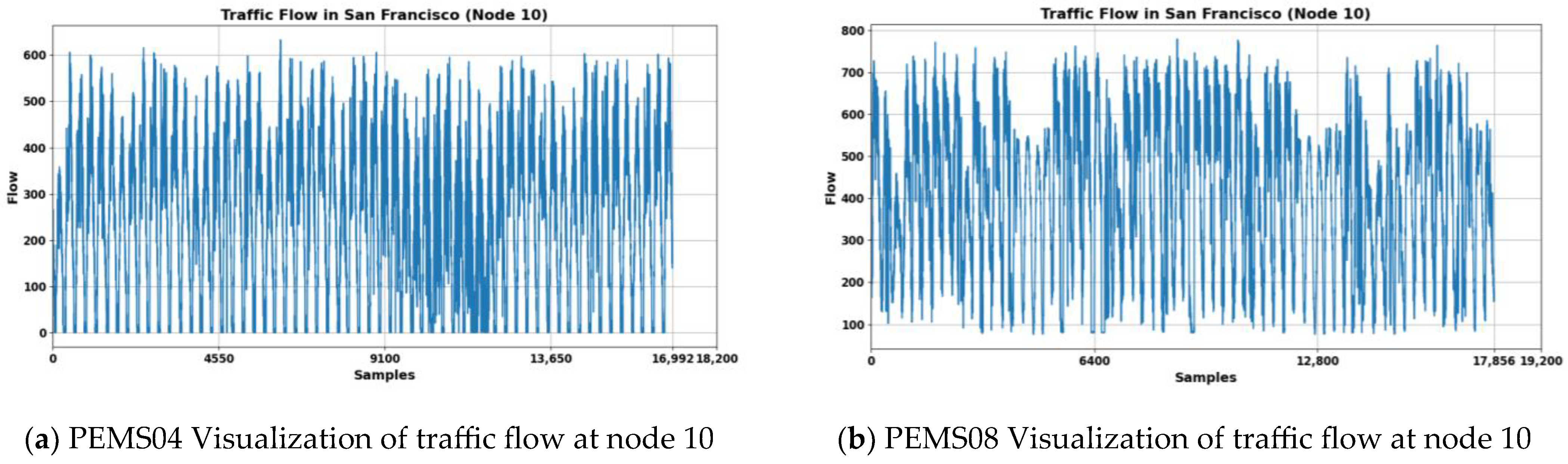
The datasets used in this paper are a set of publicly available datasets provided by the Performance Measurement System (PEMS), a California transportation management system. The PEMS04 used in this paper is data generated by 307 detectors collecting data at 5-min intervals for a total of 59 days. The PEMS08 is data generated by 170 detectors collecting data at 5-min intervals for a total of 62 days. The data collected by each detector at each acquisition contains three dimensions of features: flow, average velocity, and average occupancy. In this paper, we will retain the flow rate component for prediction experiments. 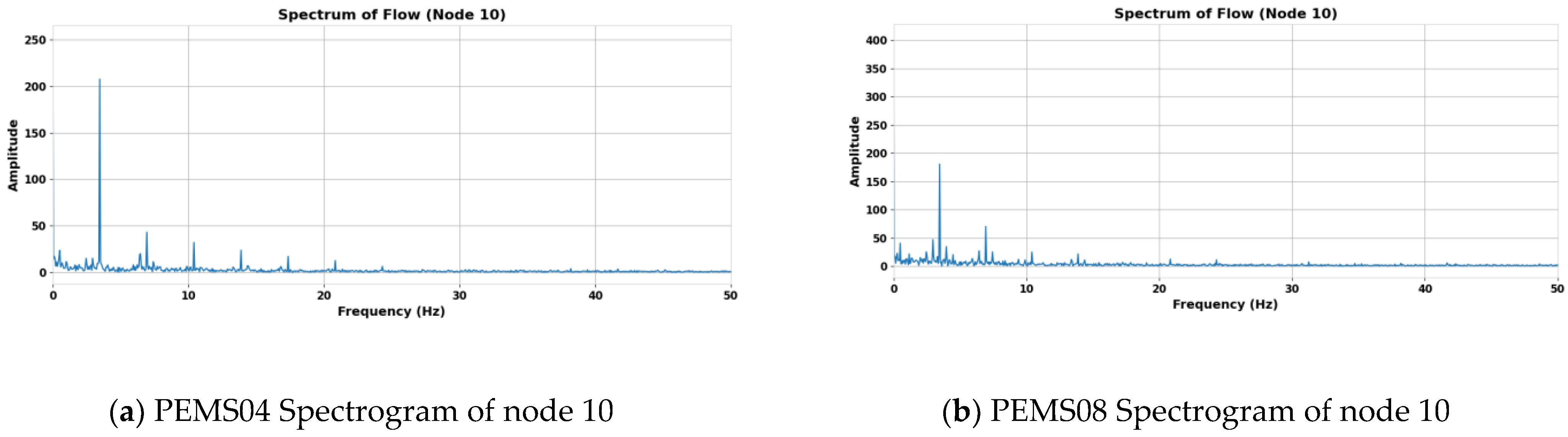The raw traffic of node 10 in both datasets is shown in Figure 2a,b, where (a) is the traffic data of node 10 of PEMS04, 16,992 is the quantity collected in 59 days at this node, and (b) is the traffic data of node 10 of PEMS08, 17,856 is the quantity collected in 62 days at this node. In the process of frequency domain feature extraction, we subjected the original traffic flow sequence to FFT, and the spectrograms of node 10 in both datasets after FFT transformation are shown in Figure 3a,b.

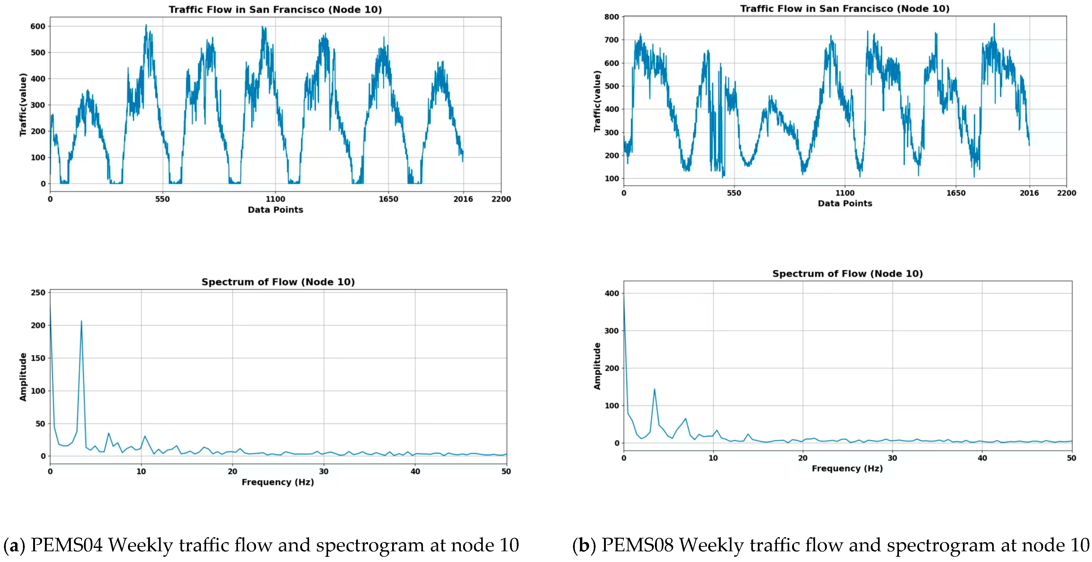
Specifically, the number of samples collected in a day is 288, and we take the traffic flow data of any week to analyze, as shown in Figure 4a,b. Analyzing from the time domain, it can be seen that a clear periodicity is presented. However, other characteristics presented in the data cannot be obtained from the time domain.

Amplitude represents the strength or energy of a signal at a specific frequency. The greater the amplitude, the more substantial the contribution of that frequency component to the signal. Amplitude is typically used to identify the dominant frequency components of the signal. Phase, on the other hand, indicates the relationship between a specific frequency component and time. Phase information is crucial for understanding the signal’s waveform, periodicity, and time delays. When multiple signals are superimposed, phase differences can cause interference, which can, in turn, affect the final shape of the signal.

4.2. Evaluation Metrics

The anomaly detection method proposed in this paper is based on flow prediction, and the accuracy of detection is related to the accuracy of prediction. The evaluation metrics are all selected as Mean Absolute Error (MAE), Root Mean Square Error (RMSE), Mean Absolute Percentage Error (MAPE). Where: $x^t$ is the observed value, ${\widehat{x}}^t$ is the predicted value, and n is the total number of samples.

MAE measures the average absolute value of the prediction errors, which represents the average deviation between the predicted values and the true values. The smaller the value, the more accurate the prediction. The calculation formula is as follows:

$$MAE={\displaystyle \frac{1}{n}}{\sum }_{t=1}^n|x^t-{\widehat{x}}^t|.$$

(24)

RMSE calculates the root mean square error, which is the square root of the average of the squared errors. Since squaring amplifies larger errors, RMSE emphasizes the impact of large errors. It is suitable for scenarios that are sensitive to large errors. The smaller the value, the better the model’s fit. The calculation formula is as follows:

$$RMSE=\sqrt{{\displaystyle \frac{1}{n}}{\sum }_{t=1}^n(x^t-{\widehat{x}}^t{)}^2}.$$

(25)

MAPE measures the percentage of the error relative to the true values, providing a dimensionless error metric. The smaller the value, the smaller the model’s prediction error. The calculation formula is as follows:

$$MAPE={\displaystyle \frac{100\%}{n}}{\sum }_{t=1}^n\left|{\displaystyle \frac{x^t-{\widehat{x}}^t}{x^t}}\right|.$$

(26)

The Nash-Sutcliffe Efficiency (NSE) coefficient is commonly used to quantify the predictive accuracy of simulation models and is widely applied in evaluating hydrological, meteorological, and environmental models. NSE is an indicator of the degree of fit between the model’s predictions and observed values. It calculates the mean square error between the predicted results and the observed values, and compares it to the variance of the observed values. The range of NSE is from −∞ to 1, with a value closer to 1 indicating better model performance. The mathematical expression for NSE is as follows:

$$NSE=1-{\displaystyle \frac{\sum _{t=1}^n(x^t-{\widehat{x}}^t{)}^2}{\sum _{t=1}^n(x^t-\overline{x^t}{)}^2}}$$

(27)

where: $x^t$ is the observed value, ${\widehat{x}}^t$ is the predicted value, and $\overline{x^t}$ is the mean of the observations.

4.3. Contrasting Models and Ablation Experiments

LSTM has been widely applied in prediction scenarios, primarily for capturing temporal dependencies. In time series forecasting tasks, it can effectively explore the time-varying features of data. For example, Abbass et al. [32] used LSTM to develop a voltage stability prediction model for power systems, while Wang et al. [33] proposed an LSTM-based ship fuel consumption prediction model using a self-attention mechanism. To capture both temporal and spatial dependencies simultaneously, CNN is used to capture spatial relationships. The combination of CNN and LSTM has become a common temporal model for traffic flow prediction [26,27,28,29,30]. To evaluate the impact of the frequency domain features proposed in this paper on prediction results, the following models were compared:

• LSTM-CNN: LSTM is a special kind of RNN that learns long-term dependent information and is widely used in sequential data processing. CNN is a class of deep learning models specialized for processing data with grid structure. Temporal deep learning + Convolutional Neural Network approach to capture both temporal and spatial correlations;
• Bi-LSTM-GAT: Bi-LSTM is a bi-directional LSTM model that achieves bi-directional reads by adding an inverse layer. GAT [17] utilizes an attention mechanism to adaptively learn the connectivity between nodes to achieve weighted aggregation of neighbors and achieve the ability to capture spatial correlations for spatial correlations with complex connectivity. This experiment captures both temporal and spatial correlations;
• LSTM-CNN-TF: Transformer [18] captures the long-range dependencies in the frequency domain through a self-attention mechanism and combines it with the classical time-domain temporal deep learning + convolutional neural network approach to realize the combined time-domain and frequency-domain prediction proposed in this paper.

4.4. Experimental Setup

In the experiment, the data from 59 days in PEMS04 is divided into a training set and a test set, with the first 45 days of data used for model training and the subsequent 14 days used for testing. In PEMS08, the data from 62 days is divided into a training set and a test set, with the first 48 days used for training and the final 14 days used for testing. For each dataset, historical data from 6 time steps (half an hour) is used to predict the traffic flow change in the next time step (5 min).

All deep learning networks in this study are implemented using Pytorch 2.3.1. The model uses the Adam optimizer with a learning rate set to 0.0001, a batch size of 64, and 50 epochs. Additionally, learning rate decay and early stopping strategies are employed to prevent overfitting.

The network parameters of the model proposed in this paper are set as follows: the number of multi-attention heads in the GAT network num_heads is 4; the number of hidden layers num_hid is 6; and the output feature dimension out_c is 6. The number of layers num_layers of Bi-LSTM is 2, the hidden layer dimension hid_c is 16, and the output feature dimension out_c is 6; Transformmer encoder has an output dimension coder_c of 8; the number of encoders and decoders num_coder are both 2, and the number of attention heads num_heads is 4. The convolutional kernel size kernel_size of the CNN is 5 in the comparison and ablation experiments.

4.5. Predicted Results

To verify the advantages of the BI-GAT-TF model proposed in this paper, a comparative experiment was conducted with the CNN-LSTM-TF prediction model. Additionally, to assess the effectiveness of the proposed frequency-domain spatial feature extraction in improving the model’s prediction accuracy, an ablation study was performed by removing the frequency-domain feature extraction module from the BI-GAT-TF model and observing the results. For a more intuitive understanding of the impact of frequency-domain feature extraction on the experimental results, a comparison was also made between the traditional CNN-LSTM model and the CNN-LSTM-TF model.

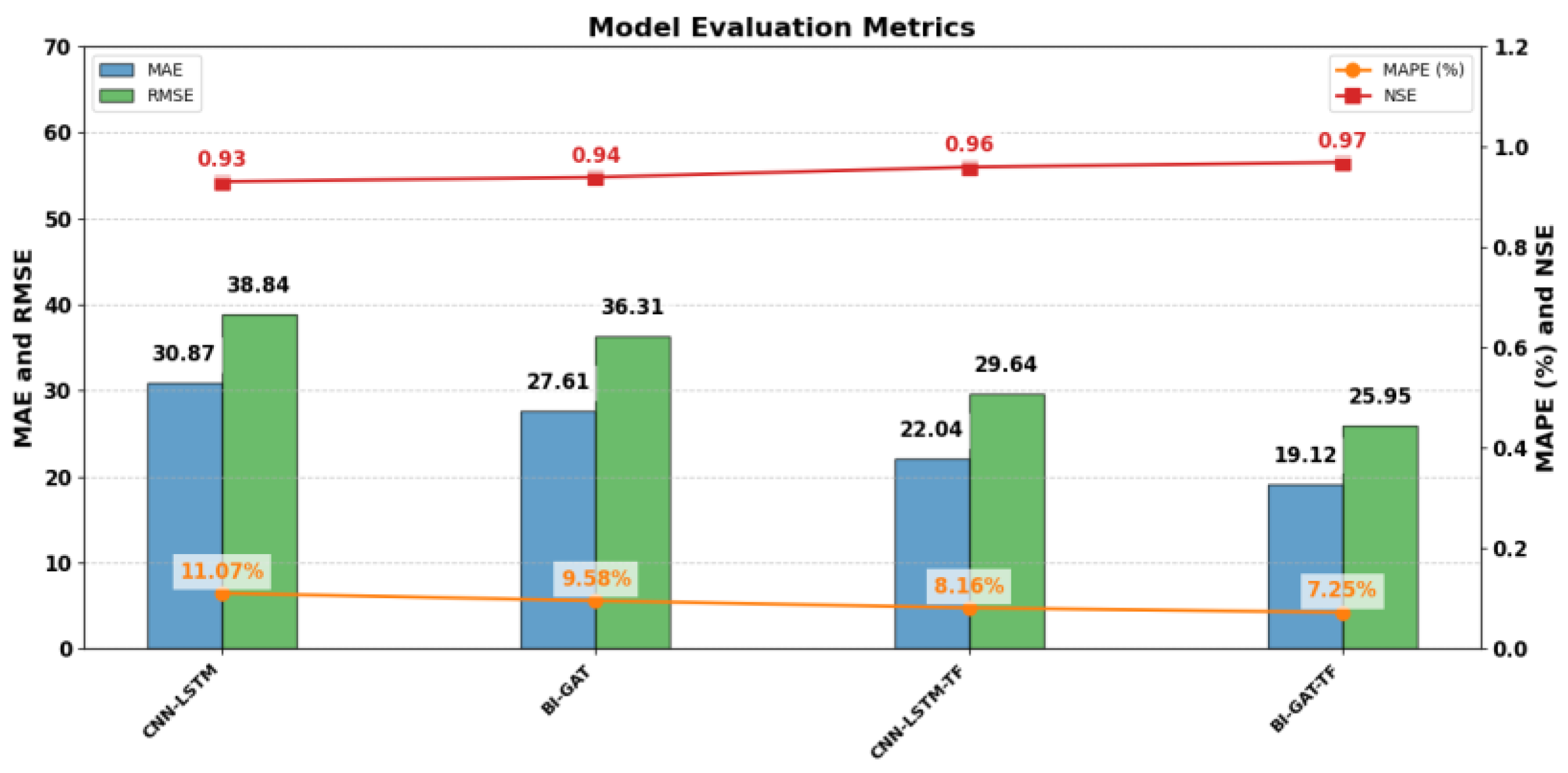
The experimental results comparing the proposed prediction model with the baseline models are shown in Figure 5 and Figure 6. From the results, the proposed model achieves the lowest MAE, MAPE (%), and RMSE on both the PEMS04 and PEMS08 datasets. Specifically, in the PEMS04 dataset, the values are 26.05, 12.36, and 37.08, while in the PEMS08 dataset, the values are 19.12, 7.25, and 19.12, respectively. The NSE is also the highest in both datasets, with values of 0.93 and 0.97, respectively. These results indicate that the proposed model achieves optimal performance in terms of prediction error and accuracy. Notably, the experimental results on the PEMS08 dataset outperform those on the PEMS04 dataset. This can be attributed to the fact that the PEMS08 dataset contains a larger number of traffic flow sequences, which provides a longer total sequence length. This increase in sequence length offers a clear advantage in terms of model training and feature extraction. In conclusion, the proposed prediction model demonstrates excellent detection performance on real-world test datasets, achieving more accurate predictions.

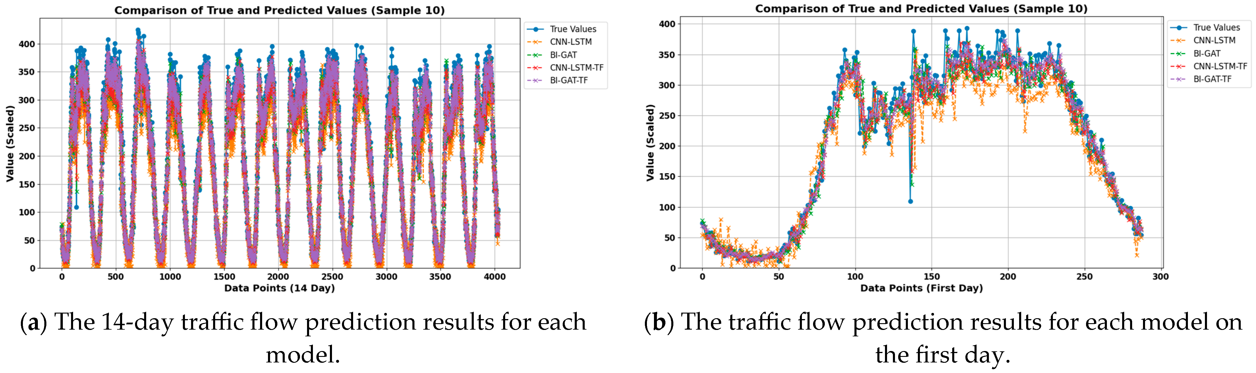
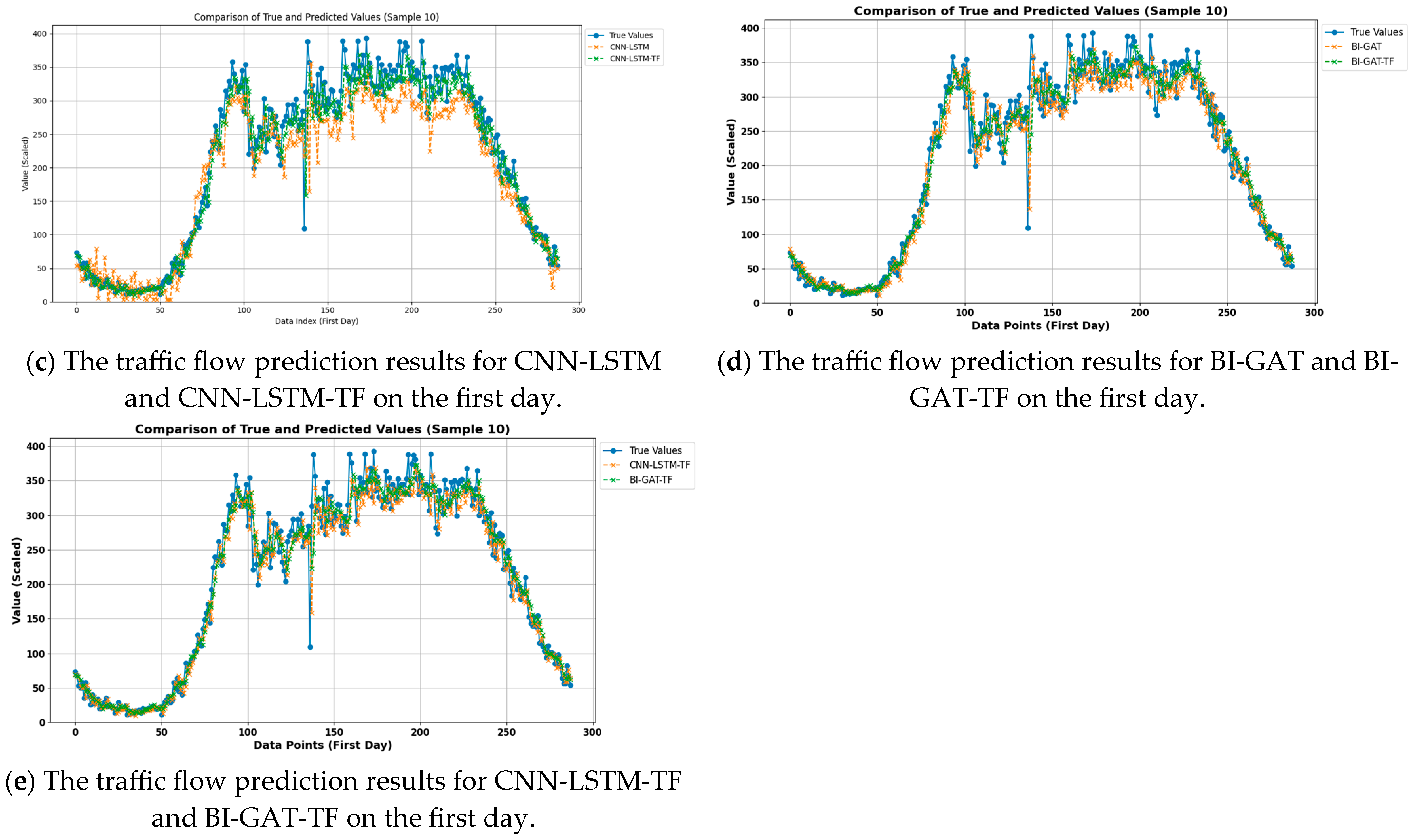
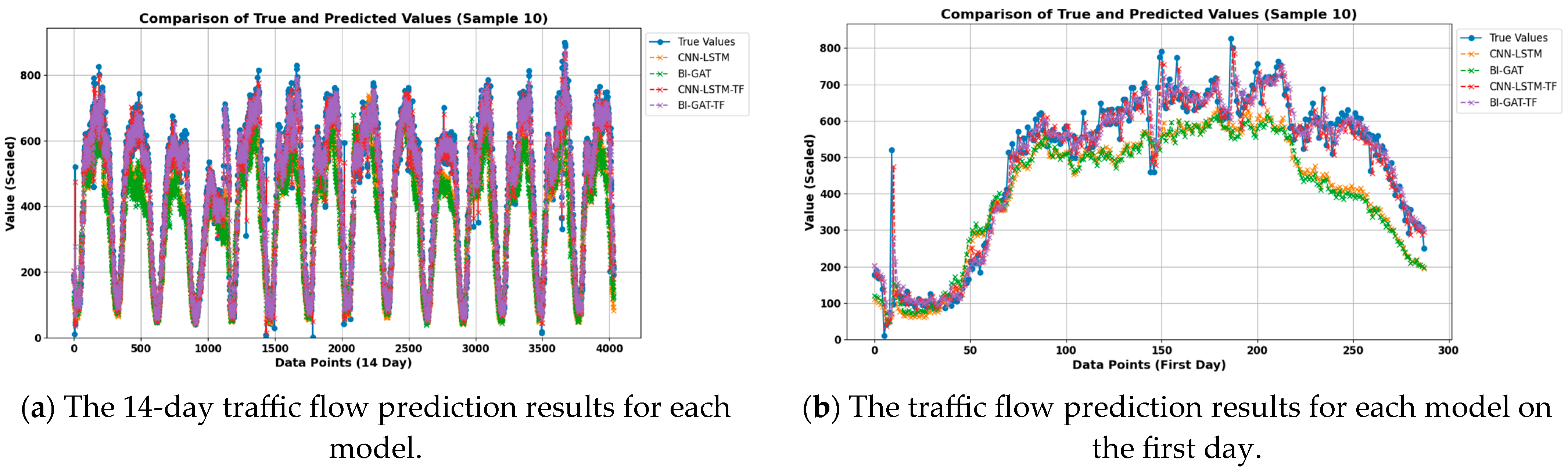
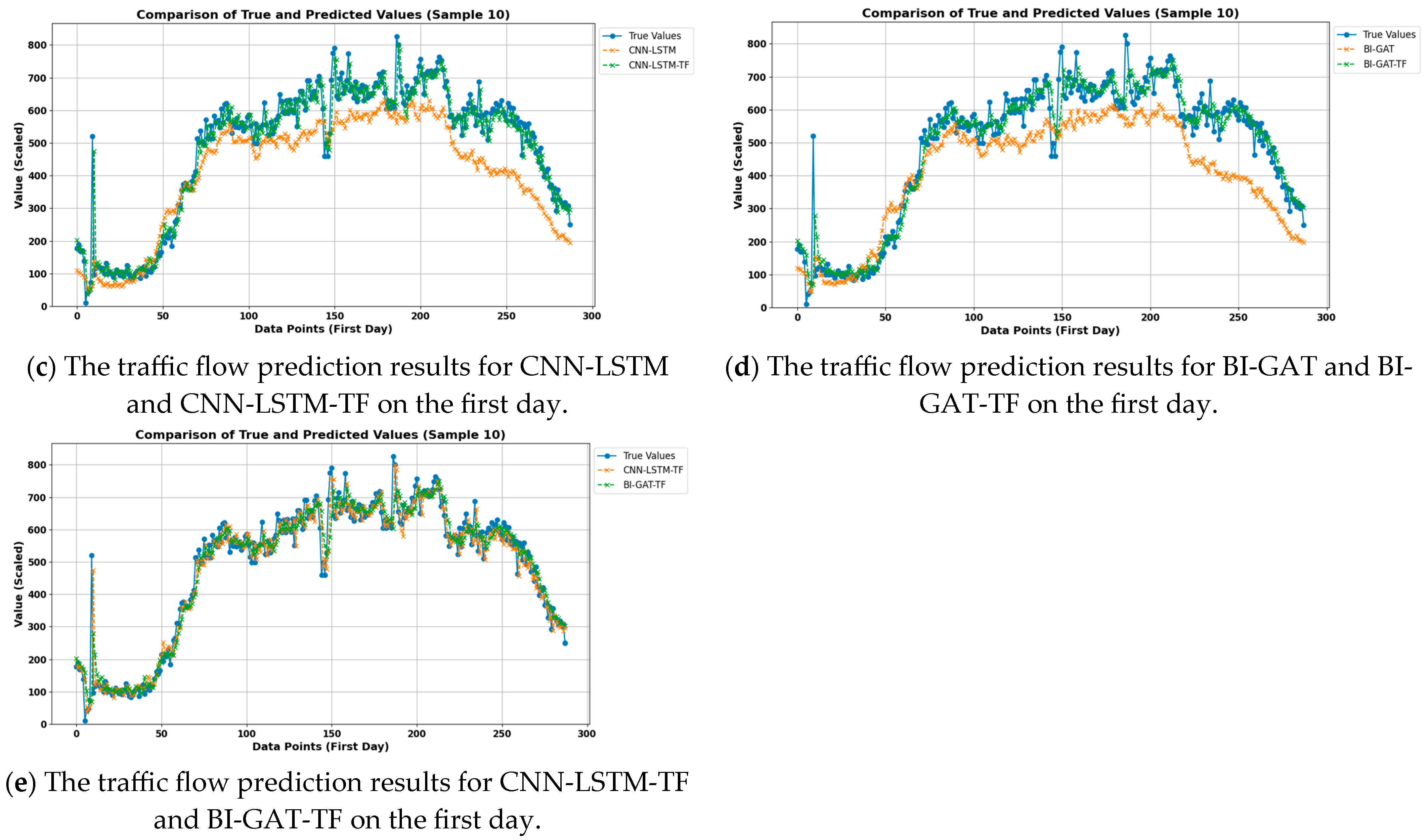
Figure 7 and Figure 8 show the experimental results for node 10 in the PEMS04 and PEMS08 datasets, respectively. (a) shows the 14-day traffic flow prediction results for each model; (b) shows the traffic flow prediction results for each model on the first day; (c) shows the traffic flow prediction results for CNN-LSTM and CNN-LSTM-TF on the first day; (d) shows the traffic flow prediction results for BI-GAT and BI-GAT-TF on the first day; (e) shows the traffic flow prediction results for CNN-LSTM-TF and BI-GAT-TF on the first day.

As shown in Figure 7c,d and Figure 8c,d, the results indicate that the prediction models with the frequency domain feature extraction module are closer to the true data. The results in Figure 7e and Figure 8e more clearly demonstrate that the BI-GAT-TF model performs better in terms of fitting compared to CNN-LSTM-TF. This suggests that the proposed model, both in terms of the selected time domain feature extraction model and the idea of frequency domain feature extraction, significantly improves the prediction accuracy of the model.

It is worth noting that, both in the PEMS04 and PEMS08 datasets, there are data points with large fluctuations, such as around noon in PEMS04 (around 12:00) and around 1 AM in PEMS08. At these times, the fitting performance of CNN-LSTM-TF is better than the other three models. However, while analyzing these points, it is important to consider not only the model’s fitting at these points but also whether the data collected at these time points may be anomalous.

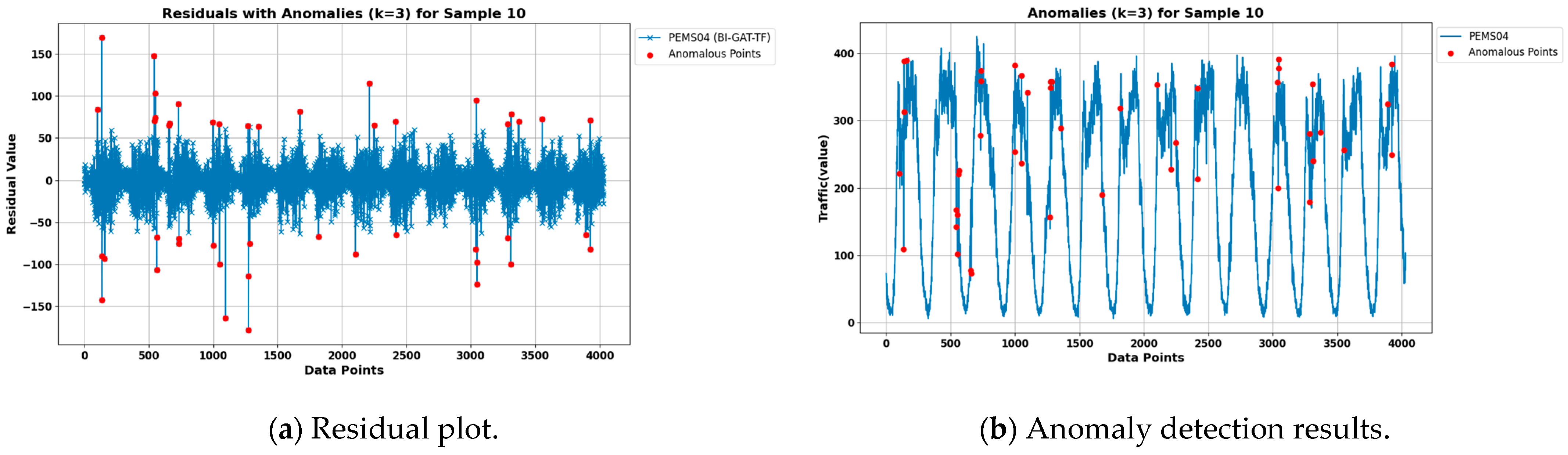
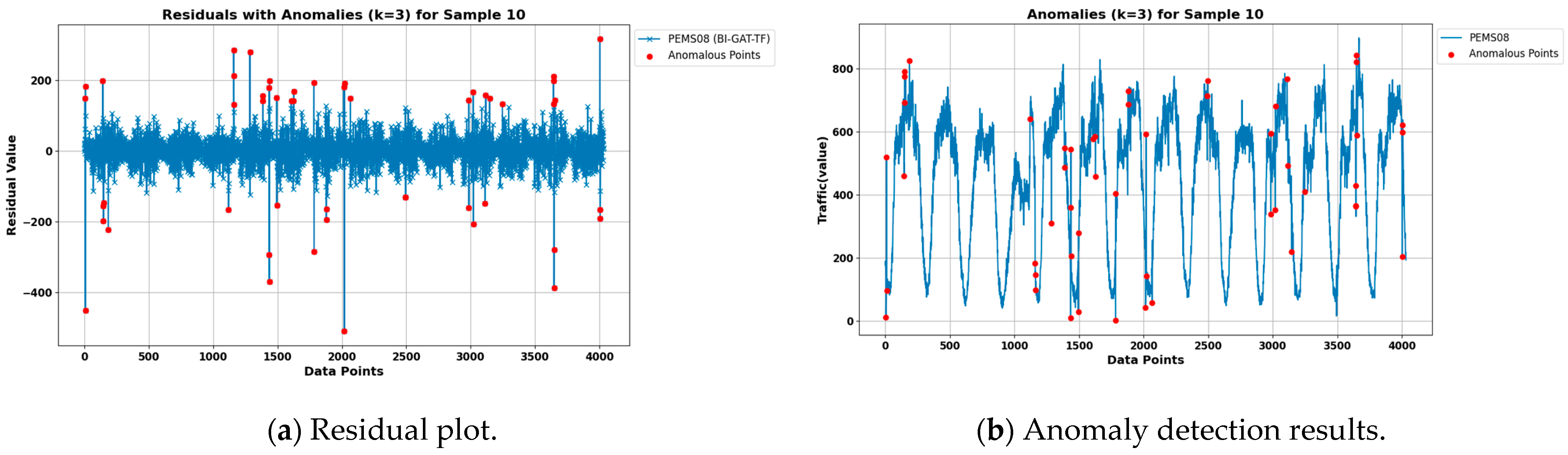
4.6. Abnormal Detection Results

The anomaly detection part first requires determining the error threshold. Set k to 3. According to Chebyshev’s inequality, an error $e_t$ exceeding ${\mu }_e+3{\sigma }_e$ or ${\mu }_e-3{\sigma }_e$ is considered to be an outlier for that data point, i.e., at least $1-{\displaystyle \frac{1}{9}}\approx 88.9\%$ of the errors should fall within the range of ${\mu }_e\pm 3{\sigma }_e$. Combined with the above proposed prediction model, anomaly detection is carried out, and the number of detected anomalies in the PEMS04 and PEMS08 datasets are 46 and 51, respectively. The detection results are shown in Figure 9 and Figure 10. Among them, Figure 9a and Figure 10a display the residual plots for the two datasets, showing the residual range when k = 3 and the detected anomalies in the residual plots. Figure 9b and Figure 10b show the anomalous points detected in the original traffic flow for the two datasets.

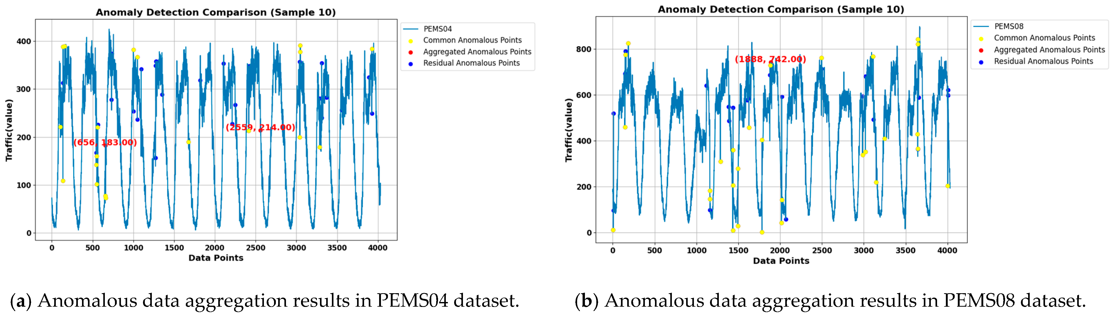
The dataset used in this paper is real traffic flow data, and there is no labeling of anomaly data. In order to more reasonably verify the effectiveness and accuracy of the detection method in this paper, this paper compares the classical unsupervised anomaly detection methods: the Ensemble-based isolated forest method [34], the reconstruction-based LSTM-VAE [35] method, and the prediction-based LSTM-NDT [36] methods, to further validate the accuracy of anomaly detection. Isolation Forest (IF) distinguishes normal and abnormal data by isolation and is suitable for high-dimensional data and large-scale datasets; LSTM-VAE captures temporal dependencies by invoking a combinatorial model that feeds potential variables learned by VAE into LSTM, and finally identifies anomalies by using the reconstruction probabilities; and LSTM-NDT predicts the anomalies by using LSTM data, detects anomalies by computing errors, and introduces an unsupervised nonparametric anomaly thresholding strategy.

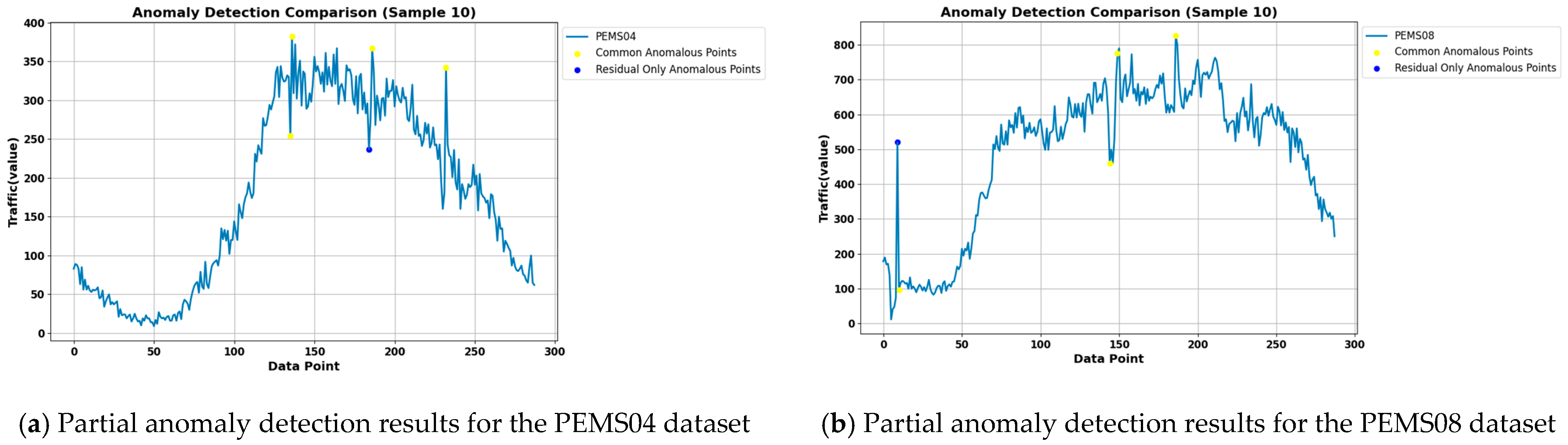
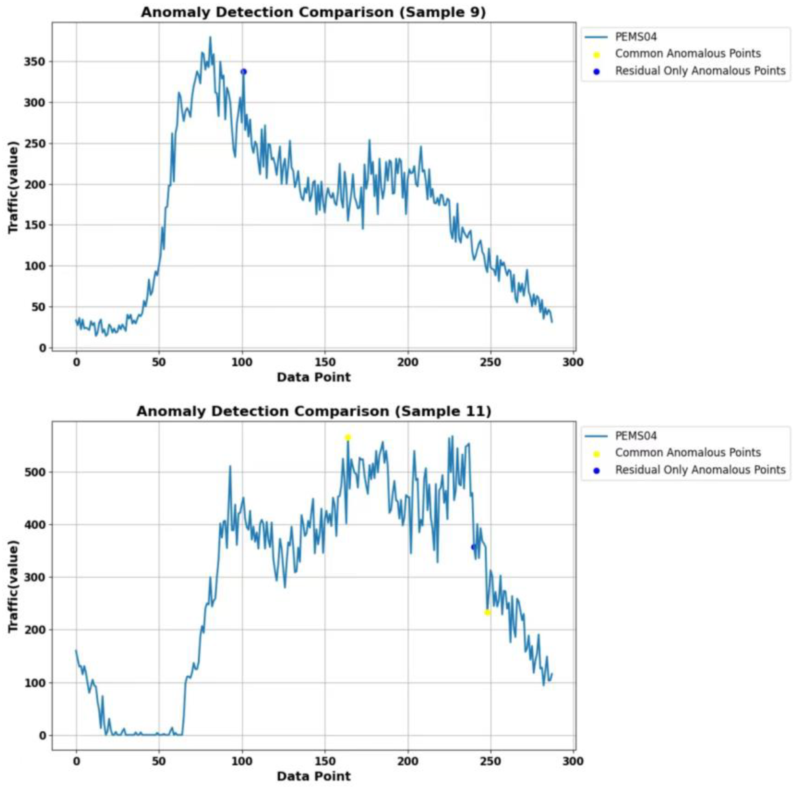
The results of the three methods, Isolation Forest, LSTM-VAE, and LSTM-NDT, are aggregated by the voting method, and at least two methods are set to consider a point as anomalous before it is considered as an anomaly. The anomalies obtained from the aggregation are compared with the anomalies detected in this paper, and the results are shown in Figure 11. The blue points in the figure are the anomalies detected using the methods in this paper and not detected by the aggregation methods, the yellow points are the common anomalies detected by the aggregation methods and also detected by the methods in this paper, and the red points are the anomalies detected by the aggregation methods and not detected by the methods in this paper.

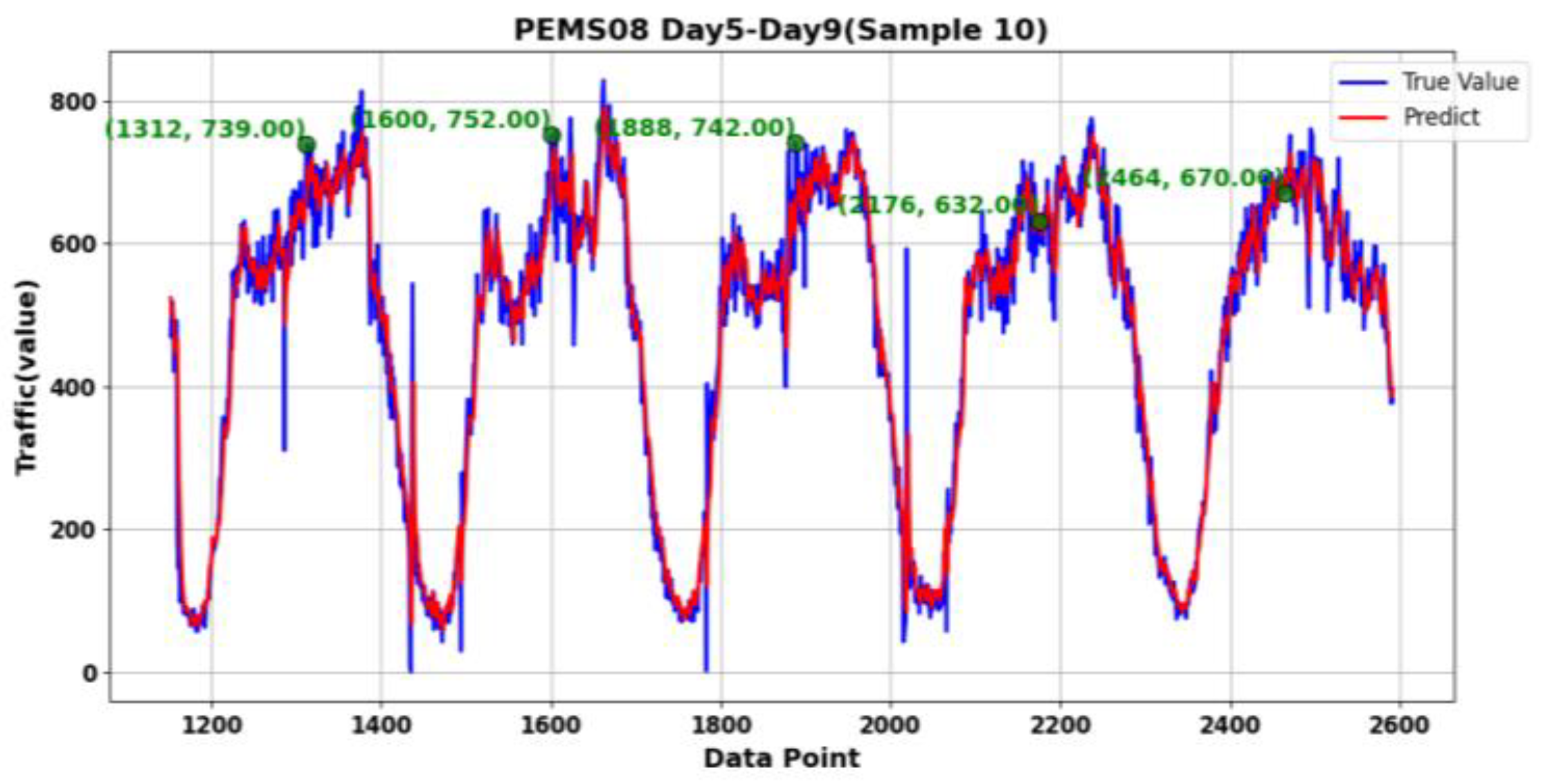
Analysis of the aggregation results shows that in the PEMS04 dataset, the number of anomalies obtained by the aggregation method is 21, and the number of anomalies obtained by this paper’s detection method is 46. Compared with the anomalies obtained by the aggregation method, this paper’s detection method detected 19 of them, and 2 data points were not detected. In the PEMS08 dataset, the number of anomalies obtained by the aggregation method is 30, and the number of anomalies obtained by the detection method in this paper is 51. Compared with the anomalies obtained by the aggregation method, the detection method in this paper detects 29 of them, and 1 data point is not detected.

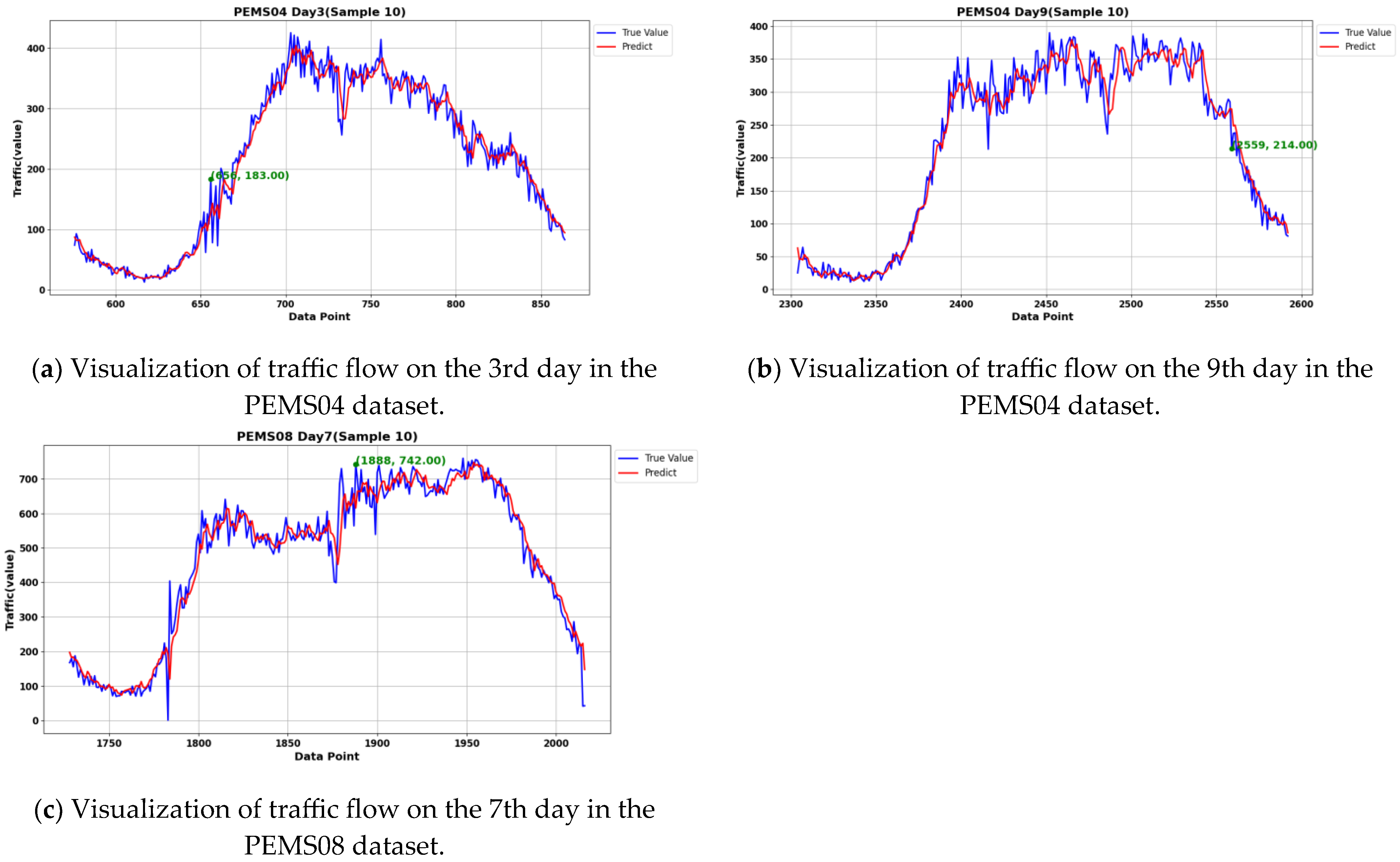
After analysis, the two data points that were not detected in this paper in the PEMS04 dataset were in the time periods of the third and ninth days. Similarly, the one data point in the PEMS08 dataset that appeared to be undetected was in the time period of the seventh day, as shown in Figure 12.

We expanded the time range and visualized the results, as shown in Figure 13 and Figure 14. Specifically, Figure 13a shows the traffic flow from the first to the fifth day in the PEMS04 dataset, while Figure 13b shows the traffic flow from the seventh to the eleventh day in the PEMS04 dataset. Figure 14 shows the traffic flow from the fifth to the ninth day in the PEMS08 dataset. The data points in the figures represent the coordinates of the data points that were not detected by our method, as well as the coordinates of the two days before and after each of these points.

Traffic flow data exhibits certain periodic patterns, such as differences in flow during peak periods (morning and evening rush hours) and off-peak periods. It may also display seasonal variations on a daily, weekly, or monthly basis. Additionally, traffic flow between adjacent road sections or intersections is often correlated, with upstream traffic conditions influencing downstream ones. The flow typically changes within a reasonable range. This characteristic can be leveraged to further assess whether the undetected data points are truly anomalies. The undetected data points in the figures, however, do not show any significant abnormalities and remain within a reasonable range of variation.

An analysis of the anomalies detected by the proposed method but missed by the aggregation method reveals that the proposed detection method identifies more anomalies with clear abnormal characteristics that do not align with short-term traffic flow changes, as shown in Figure 15. The reason for this result, aside from the aggregation method causing the loss of a few anomalies, primarily lies in the limitations of the aforementioned anomaly detection methods when handling high-dimensional and time-series data. For instance, the Isolation Forest method assumes that features are independent, but in time-series data, temporal dependencies (such as trends or seasonality) are crucial, and it fails to model these temporal relationships. LSTM-VAE, while effective, requires complex training and substantial time and computational resources, especially for long time series or high-dimensional data. Its training efficiency is relatively low, and when the difference between anomalies and normal data is small, the model may struggle to differentiate between the two. LSTM-NDT assumes that the prediction errors of normal data are small, while those of anomalies are larger. However, by modeling only temporal features, it fails to adequately learn the data’s full characteristics, leading to poor performance of the prediction model and reduced error differentiation ability, which negatively impacts anomaly detection.

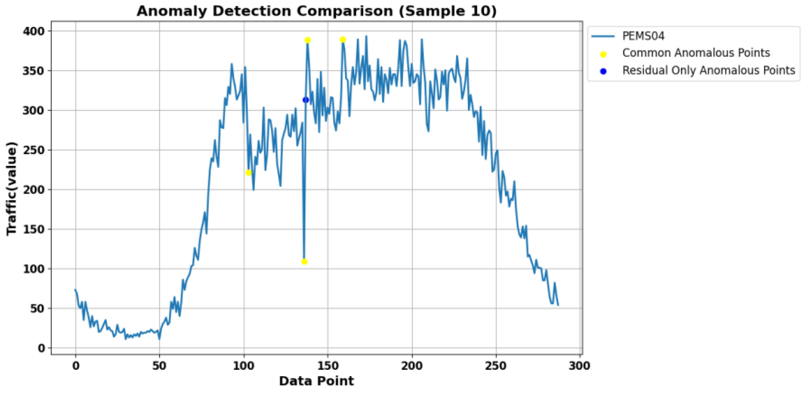
Additionally, the proposed detection method in this paper also identifies cases where the difference between two anomalous data points within a short time span is too large, and it classifies the data between these anomalies as abnormal, as shown in Figure 16. The dataset in this study is collected every 5 min, and based on the analysis of traffic flow variation characteristics, significant changes in traffic flow within a short period may be caused not only by anomalies in data collection but also by the occurrence of unexpected events.

To verify whether the drastic fluctuations in traffic flow during this time period were caused by a sudden event, we analyzed the basic relationship between upstream and downstream traffic flow. The relationship between upstream and downstream traffic flow is highly dynamic and coupled. Upstream flow affects downstream flow through a transmission effect, while downstream flow can also influence upstream flow through a feedback effect. We observed the flow changes of nodes connected to this particular node during this time period, as shown in Figure 17. From Figure 17, there were no significant changes in the upstream and downstream traffic flow during this period, making the likelihood of a sudden event minimal. Based on practical considerations, if abnormal data is detected both at the beginning and end of a short data collection period, the data measured during this short period is most likely also abnormal. Thus, the situation where two anomalous data points within a short time frame have a large discrepancy, and the data between these points is also classified as abnormal, aligns better with real-world scenarios. This analysis further validates that the anomaly detection method proposed in this paper has higher accuracy.

5. Conclusions

This paper proposes a traffic flow anomaly detection method based on predictive multi-domain feature extraction. The method reduces prediction errors by constructing a more accurate prediction model and determines the error threshold using Chebyshev’s inequality. Anomalous data points are identified by checking whether the prediction error falls within the threshold range. Experimental results demonstrate that optimizing the prediction model and improving the error analysis method can effectively enhance the accuracy of anomaly detection.

In terms of prediction model improvement, the proposed approach fully leverages the characteristics of traffic flow data and incorporates both time-domain and frequency-domain features for time series modeling. In the time domain, the model captures temporal and spatial correlations of the time series, while in the frequency domain, it extracts amplitude and phase information to learn frequency-related characteristics. Experimental results on the PEMS04 and PEMS08 datasets show that the prediction accuracy of the multi-domain feature extraction model is significantly higher than that of methods relying solely on time-domain features. This conclusion remains valid even when compared with the classical CNN-LSTM model.

In terms of error analysis and error threshold determination, this paper innovatively introduces Chebyshev’s inequality to establish the error threshold. By determining whether the error exceeds this threshold, a more scientific and rational error analysis is achieved, enhancing the accuracy and robustness of anomaly detection. As a result, potential anomalies within the dataset are effectively identified. Finally, a comparison with classical unsupervised anomaly detection methods is conducted to more reasonably validate the accuracy of the proposed method in detecting anomalies within unlabeled datasets.

We also note that the dataset used in this paper has some limitations, such as less missing data, lower proportion of noise, and so on. In the future, we can conduct experiments under the conditions of having clear outlier labels, adding different proportions of noise, etc., comparing more benchmark models, etc., to continuously improve the detection accuracy.