REU-Net: A Remote Sensing Image Building Segmentation Network Based on Residual Structure and the Edge Enhancement Attention Module

Abstract

Building segmentation from high-resolution remote sensing images plays a crucial role in cadastral measurement, ecological monitoring, urban planning, and other applications. To address the current challenges in building segmentation from high-resolution remote sensing images, this paper proposes an improved deep learning-based network—REU-Net(2EEAM). The network replaces traditional convolutional blocks in U-Net with Residual Structures, deepening the network and alleviating the issue of vanishing gradients. Additionally, it substitutes the direct skip connections with two Edge Enhancement Attention Modules (EEAMs), enhancing the network’s ability to extract building edge information. Furthermore, a hybrid loss function combining edge consistency loss and binary cross-entropy loss is used to train the network, aiming to improve segmentation accuracy. Experimental results show that REU-Net(2EEAM) achieves optimal performance across multiple evaluation metrics (such as P, MPA, MIoU, and FWIoU), particularly excelling in the accurate recognition of building edges, significantly outperforming other network models. This method provides a reliable foundation for the further optimization of building segmentation algorithms for remote sensing images.

1. Introduction

The application of semantic segmentation in remote sensing image interpretation has become a crucial link between basic and advanced remote sensing image processing and analysis. This technology significantly enhances the accuracy of remote sensing data interpretation and provides critical technical support for interdisciplinary applications. Remote sensing images, as key carriers of land feature information, contain substantial economic and social value within their data. In remote sensing image analysis, the in-depth exploration and utilization of this information is central to research [1]. Digital image processing techniques enable the efficient extraction of rich information from remote sensing images, which is crucial for various fields, such as cadastral surveying, ecological environment monitoring, and urban planning. Semantic segmentation, by dividing images into multiple regions with specific attributes, can accurately identify target objects or features. It has demonstrated significant applications in various fields, such as geographic information systems (GISs), autonomous driving, robotics, and medical image recognition. However, due to the inherent diversity of categories and the complexity of detailed features in remote sensing images, as well as significant redundancy across different spectral bands, traditional shallow models often struggle to achieve optimal feature extraction results. At the same time, the accuracy of traditional remote sensing image semantic segmentation methods remains relatively low. Therefore, improving the accuracy of target extraction in remote sensing images has become a key and challenging topic in current remote sensing research and technological development [2,3].

Classic remote sensing image segmentation methods primarily rely on low-level image features, such as color and shape, to design a set of features, which are then combined with an existing feature library for automatic target recognition and extraction. Thresholding, edge detection, and region-based segmentation are common methods for image segmentation. Thresholding segmentation [4,5,6] selects a threshold based on the image’s grayscale features, effectively separating the target from the background with high computational efficiency. Due to the inherent feature of regional discontinuity in remote sensing images, edge detection segmentation can be employed to perform image segmentation based on this characteristic. Chen, J. et al. [7] detected edge features in multi-spectral remote sensing images and combined them with multi-scale segmentation techniques to control the merging process of adjacent objects. Chen, B. et al. [8] added an edge penalty term, which not only ensures the accurate segmentation of large objects in remote sensing images but also effectively identifies smaller objects. Lakshmi, S. et al. [9] used differential operators for edge detection in their study and proposed an image segmentation method based on edge detection. Zhao, M. et al. [10] proposed a co-occurrence matrix from the grayscale perspective, combining regional feature information with image edge information to improve segmentation accuracy. However, the information contained in remote sensing images is complex, and these segmentation algorithms are susceptible to interference from factors, such as lighting and sensors, resulting in limited robustness. They are only capable of handling simple, specific data and are not efficient or precise enough for building extraction. Machine learning-based segmentation algorithms have somewhat alleviated these issues. However, traditional machine learning classifiers (such as AdaBoost, support vector machines (SVMs), and random forests) used for building feature extraction typically require post-processing steps to refine the segmentation results [11,12,13]. These methods not only have high model complexity and require substantial human–machine interaction but are also often limited by the constraints of human knowledge and experience.

Deep learning, an advanced method within the field of machine learning, has found widespread applications in remote sensing and computer vision. Numerous researchers have conducted extensive studies in these fields using this technology. Krizhevsky, A. et al. [14] introduced the AlexNet model, which was the first to integrate the ReLU activation function and the Dropout strategy into the architecture of convolutional neural networks (CNNs). They also applied GPU acceleration to the training and testing processes of the network. Long, J. et al. [15] proposed the Fully Convolutional Network (FCN), an innovative architecture. The breakthrough of this method lies in its ability to achieve end-to-end learning for image segmentation tasks, where feature images are directly input, and the corresponding outputs are generated. This innovation not only improves the computational efficiency of semantic image segmentation but also enhances segmentation accuracy. However, Fully Convolutional Networks (FCNs) have certain limitations in image segmentation tasks. While the network performs well in pixel-level classification tasks, it primarily focuses on the independent classification of individual pixels. It does not fully consider the spatial relationships between pixels and the correlation of pixel values, leading to segmentation results that lack spatial consistency. To address this issue, researchers have focused on optimizing the network architecture, improving the model’s ability to capture the spatial relationships and value correlations between pixels to enhance segmentation performance. U-Net, proposed by Ronneberger, O. et al. [16] in 2015, is a variant of the Fully Convolutional Network (FCN). The network features a symmetric architecture, extracting both low-level and high-level features. By introducing skip connections, U-Net enables the fusion of feature maps at the same scale between the encoder and decoder. However, this method requires strict consistency in feature scales and is challenging to directly determine the optimal depth in practical applications. Zhou, Z. et al. [17] proposed UNet++ to address the limitations of traditional U-Net in segmenting objects of varying scales. By introducing nested and dense skip connections, UNet++ significantly improves segmentation accuracy and achieves faster convergence. In addition to improving the network architecture, some researchers have actively explored new methods and techniques to combine with the U-Net model to enhance its performance and efficiency. Tang, P. et al. [18] addressed the overfitting issue in U-Net segmentation results by proposing a random weighted averaging method, which achieved a broader optimal solution and improved generalization. He, N.J. et al. [19] tackled the issue of CNNs neglecting the correlations between intermediate features in building segmentation by proposing a hybrid first- and second-order attention network (HFSA). This network adaptively re-scales intermediate features by leveraging global averages and inner products between different channels, making the features more representative.

The key challenge in high-resolution remote sensing image segmentation for buildings lies in distinguishing building pixels from background pixels. However, during segmentation, interference from adjacent factors, such as bridges, shadows, riverbanks, and road-like structures makes it difficult to establish an efficient segmentation model, especially at the boundaries of the segmented targets where accurate results are hard to achieve. To address these issues, this study applies deep learning to building extraction from remote sensing images and proposes a building segmentation network named REU-Net. This network combines residual structures with an Edge Enhancement Attention Module to improve segmentation performance. The network is based on U-Net, with the following three main optimization strategies:

• The traditional 3 × 3 and 1 × 1 convolution blocks in the U-Net encoder are replaced with residual (Res) modules. This deepens the network structure, alleviates the vanishing gradient problem, and effectively transfers features from one layer to the next, enabling the extraction of deeper semantic information.
• The direct skip connections are replaced with an Edge Enhancement Attention Module (EEAM). This module enhances the extraction of contour and edge information of buildings by calculating the difference between positional features and original features, thus improving segmentation accuracy.
• A hybrid loss function combining edge consistency loss and binary cross-entropy loss is proposed, tailored to the characteristics of building segmentation in remote sensing images. This function helps the model capture building contours of varying sizes and shapes, distinguish buildings from the environment and background, and enhance the performance of the segmentation network.

2. Segmentation Model

Convolutional Neural Networks (CNNs) are a type of feedforward neural network with a deep structure that incorporates convolution operations, and they are one of the key algorithms in deep learning. CNNs combine low-level features to form abstract high-level features. As the number of attribute categories in the data increases, the network often applies more non-linear operations, such as activation functions. Deep CNNs apply a series of convolution, deconvolution, and pooling operations to extract and transform features from the raw input data layer by layer. This allows the network to automatically learn hierarchical feature representations, resulting in improved performance in tasks, such as image segmentation and feature visualization.

U-Net, as a type of deep convolutional neural network, employs a symmetric network structure for the stepwise extraction of shallow and deep features. It consists of an encoder and a decoder, formed by a series of convolution and pooling operations, positioned on the left and right sides of the network. The encoder extracts shallow features and performs dimensionality expansion on the image matrix, while the decoder gradually reduces dimensionality and performs upsampling. The resulting deep features are linked across the same layer using skip connections, and the network finally outputs binary or multi-class predictions. Due to the limitations of the network structure, U-Net faces challenges in semantic segmentation, particularly in the early stages of shallow feature extraction. It struggles to fully transfer features from one layer to the next. Additionally, in skip connections, the direct linking method fails to effectively eliminate random noise caused by misjudgments in the network. To address these issues, we introduce the following modules: the Residual (Res) module and the Edge Enhancement Attention Module (EEAM). The structure of REU-Net is shown in Figure 1.

2.1. Design of REU-Net Model Structure

The traditional U-Net is highly praised for its clear structure and excellent performance on small sample datasets. The original U-Net consists of 18 3 × 3 convolution layers, 1 1 × 1 convolution layer, 4 2 × 2 downsampling layers, and 4 2 × 2 upsampling layers, with ReLU used as the activation function. However, after several convolution operations on the left side of the model (the initial feature extraction part), there is a significant loss of feature elements, which hinders the complete and effective extraction of primary features. Additionally, noise handling is not optimized. Since this research aims to detect buildings effectively in remote sensing image datasets, we propose an optimized REU-Net model. The specific structure of the model is shown in Figure 2. The specific optimization of the network mainly includes the following two components.

The ResBlock module [20] is introduced in the left encoding network part, as shown in Figure 1. When the number of channels in the previous and subsequent layers is the same, the feature map x is directly connected. When the channel numbers differ, a 1 × 1 convolution with no bias and full padding is used for dimension adjustment. This results in a new W(x), which is then added to the convolutional feature map, effectively preserving the primary features.

In the direct skip connection part of the network, the traditional direct connection is replaced with an Attention module. This module extracts edge features from the feature maps obtained at each layer and uses weighting methods to guide the feature maps of different depths from the encoding part. These guided feature maps are then combined with the upsampled feature maps, which have reduced dimensions, to recover specific pixel-level details, enabling selective and thorough feature extraction.

Specifically, we replace the original direct skip connections with EEAM at two intermediate layers (e.g., between the second and third downsampling layers and the corresponding upsampling layers). This placement is chosen because of the following: (1) Shallow Layers: The early layers capture fine-grained edge features, where EEAM enhances contour extraction. (2) Intermediate Layers: Deeper layers encode semantic information, and EEAM here suppresses noise while preserving structural details.

We experimented with inserting EEAM at different depths (1EEAM, 2EEAM, etc.), and found that using two modules optimally balances feature enhancement and computational overhead.

2.2. Edge Enhancement Attention Module

The concept of the Attention mechanism is inspired by human visual attention, essentially enabling the more precise extraction of specific features in neural networks by assigning a series of attention weight coefficients. Mnih, V. et al. [21] were the first to introduce the Attention mechanism into RNN models for image classification tasks, achieving impressive performance. Since then, Attention mechanisms have been applied to various tasks, including text processing and machine translation. Vaswani, A. et al. [22] proposed the Transformer, a network structure entirely based on the Attention mechanism, which demonstrated significant advantages in both quality and parallelism, leading to a peak in the application of Attention mechanisms.

In the dataset used in this paper, the contrast between building and non-building regions is not significant in certain areas. In such cases, directly connecting the feature output by the encoder module with the feature map obtained after deconvolution and upsampling would result in primary features that have not been noise-filtered, potentially interfering with the final output and reducing prediction accuracy. To address this, we introduce an attention mechanism into the skip connection module of U-Net to suppress the interference of non-building pixels on the feature extraction results at each layer, enhance edge feature extraction, and improve building segmentation accuracy. Based on the characteristics of the remote sensing image building segmentation task, we propose an edge-enhanced attention mechanism module, which is divided into two parts: (1) edge feature extraction and (2) feature fusion.

2.2.1. Edge Feature Extraction

A key step in the overall design of the Edge Enhancement Attention Module is the extraction of edge features, as shown in Figure 3, where each layer after upsampling is input into this module. The input features are first encoded in two directions, allowing for the full acquisition of the building’s location information. Based on this, the boundary differences are enhanced, ensuring that the final output feature map contains rich spatial awareness and strong boundary contours, thus improving the final segmentation results of building remote sensing images. The specific steps are as follows:

• Step 1. Extraction

Given an input feature $\mathrm{Z}$ with dimensions $\mathrm{h}\times \mathrm{w}$, perform max pooling along both the horizontal and vertical directions to obtain the encoded information on the vertical and horizontal structures of the input feature, respectively, which is represented as follows:

$${\mathrm{f}}_{\mathrm{w}}=\underset{0\le \mathrm{i}\le \mathrm{W}}{\max }\mathrm{Z}\left(\mathrm{h},\mathrm{i}\right)$$

(1)

$${\mathrm{f}}_{\mathrm{h}}=\underset{0\le \mathrm{i}\le \mathrm{H}}{\max }\mathrm{Z}\left(\mathrm{i},\mathrm{w}\right)$$

(2)

Here, $\mathrm{Z}$ denotes the input feature map with dimensions $\mathrm{h}\times \mathrm{w}$, $\mathrm{h}, \mathrm{w}$ represents the height and width of the feature map $\mathrm{Z}$ respectively, and $\mathrm{H}, \mathrm{W}$ represents the maximum of feature map $\mathrm{Z}$’s height and width, respectively.

• Step 2. Transformation

After concatenating the features from the two directions, they are passed through a $1\times 1$ convolution F, resulting in feature maps that capture spatial information from both directions. Additionally, to accelerate the model’s convergence and enhance focus on the target region, a non-linear normalization operation is applied to the fused feature map, as follows:

$$\mathrm{U}=\mathrm{Relu}\left(\mathrm{BN}\left({\mathrm{conv}}_{1\times 1}\left(\mathrm{concat}\left({\mathrm{f}}_{\mathrm{w}}^{\mathrm{T}},{\mathrm{f}}_{\mathrm{h}}\right)\right)\right)\right)$$

(3)

Here, $\mathrm{T}$ denotes the transpose operation, concat represents the concatenation operation, conv refers to the convolution operation, BN stands for batch normalization, ReLU is the non-linear activation function, ${\mathrm{conv}}_{1\times 1}$ represents 1 × 1 convolution operation, ${\mathrm{f}}_{\mathrm{w}}$ denotes the max-pooled feature vector along the width dimension (horizontal encoding), and ${\mathrm{f}}_{\mathrm{h}}$ denotes the max-pooled feature vector along the height dimension (vertical encoding).

• Step 3. Stimulation

The fused features are divided into feature vectors for the two directions. A $1 \times 1$ convolution is used to obtain the activated directional features ${\mathrm{g}}_{\mathrm{h}}$ and ${\mathrm{g}}_{\mathrm{w}}$, and the sigmoid function is applied to map the feature values to weight values within the range $[0, 1]$.

$$\left({\mathrm{g}}_{\mathrm{h}},{\mathrm{g}}_{\mathrm{w}}\right)=\mathrm{split}\left(\mathrm{U}\right)$$

(4)

$${\mathsf{\phi }}_{\mathrm{h}}=\mathrm{sigmoid}\left({\mathrm{conv}}_{1\times 1}\left({\mathrm{g}}_{\mathrm{h}}\right)\right)$$

(5)

$${\mathsf{\phi }}_{\mathrm{w}}=\mathrm{sigmoid}\left({\mathrm{conv}}_{1\times 1}\left({\mathrm{g}}_{\mathrm{w}}\right)\right)$$

(6)

By performing a matrix multiplication, the weight information from the horizontal and vertical directions is combined to obtain the weight for each position in the spatial domain. This weight is then applied to the original image to obtain the spatially weighted feature attention, as follows:

$$\mathrm{V}\left(\mathrm{i},\mathrm{j}\right)=\mathrm{Z}\left(\mathrm{i},\mathrm{j}\right)·{\mathsf{\phi }}_{\mathrm{h}}\left(\mathrm{i},\mathrm{j}\right)·{\mathsf{\phi }}_{\mathrm{w}}\left(\mathrm{i},\mathrm{j}\right)$$

(7)

where ${\mathsf{\phi }}_{\mathrm{h}}, {\mathsf{\phi }}_{\mathrm{w}}$ refers to spatial attention weights for the height and width directions, respectively, and $\mathrm{V}$ represents spatially weighted feature map after applying ${\mathsf{\phi }}_{\mathrm{h}}$ and ${\mathsf{\phi }}_{\mathrm{w}}$.

2.2.2. Feature Fusion

After completing edge feature extraction, the features from the original channels are combined with the edge features to obtain the edge-enhanced feature information, as shown in Figure 4. The original feature map Z is fused with the edge feature attention V to obtain the edge-enhanced attention, as follows:

$${\mathrm{Z}}^{\prime }=\mathrm{Z}+\mathrm{V}$$

(8)

2.3. Loss Function Construction

In remote sensing images, buildings vary in shape, size, and appearance, making it challenging for a single loss function to capture multi-scale features effectively. Additionally, buildings in different environments and lighting conditions may be affected by noise, shadows, or occlusions, further complicating edge detection. To address these challenges, this study proposes a hybrid loss function that combines edge consistency loss with binary cross-entropy (BCE) loss. This approach enhances the model’s ability to capture building contours of various sizes and shapes while improving the distinction between buildings and their surrounding environment, ultimately increasing segmentation accuracy.

The specific definition of the loss function is given by the following equation:

$${\mathrm{Loss}}_{\mathrm{total}}=\mathsf{\alpha }·{\mathrm{Loss}}_{\mathrm{EC} }+\mathsf{\beta }·{\mathrm{Loss}}_{\mathrm{BCE}}$$

(9)

Here, ${\mathrm{L}\mathrm{o}\mathrm{s}\mathrm{s}}_{\mathrm{E}\mathrm{C}}$ represents the edge consistency loss, and ${\mathrm{L}\mathrm{o}\mathrm{s}\mathrm{s}}_{\mathrm{B}\mathrm{C}\mathrm{E}}$ denotes the binary cross-entropy (BCE) loss. The parameters control $\mathsf{\alpha }$ and $\mathsf{\beta }$, which are the relative contribution of each loss component.

2.3.1. Edge Consistency Loss

Edge consistency loss is commonly used in image processing, computer vision, and other fields that rely on spatial structure, such as deep learning-based image reconstruction and segmentation tasks [23]. The loss is defined as follows:

$${\mathrm{Loss}}_{\mathrm{EC} }={‖\nabla \widehat{\mathrm{y}}-\nabla \mathrm{y}‖}_1$$

(10)

Here, $\widehat{\mathrm{y}}$ represents the model’s predicted output, while $\mathrm{y}$ denotes the ground truth. $\nabla \widehat{\mathrm{y}}$ and $\nabla \mathrm{y}$ refer to the gradients of the predicted and true values, respectively. These gradients capture pixel-wise variations in the image and are commonly used to detect edges or transitions between different regions. ${‖·‖}_1$ represents the L1 norm, which computes the total absolute error in edge prediction.

Thus, the edge consistency loss penalizes discrepancies between the gradients of the predicted and ground truth values. In other words, any errors in the predicted edges of segmented objects are backpropagated to the model, enabling it to adjust its parameters and improve edge segmentation accuracy.

The gradient operator is a key component of the edge consistency loss. In this study, we use the Sobel operator, which is implemented through convolution layers in deep learning. The corresponding convolution kernels are as follows.

$${\mathrm{G}}_{\mathrm{x}}=\left[\begin{array}{ccc}-1& 0& 1\\ -2& 0& 2\\ -1& 0& 1\end{array}\right], {\mathrm{G}}_{\mathrm{y}}=\left[\begin{array}{ccc}-1& -2& -1\\ 0& 0& 0\\ 1& 2& 1\end{array}\right]$$

(11)

By applying convolution operations, the horizontal gradient ${\nabla }_{\mathrm{x}}$ and vertical gradient ${\nabla }_{\mathrm{y}}$ of the image can be computed separately and then combined to obtain the total gradient:

$$\nabla =\sqrt{{\left({\nabla }_{\mathrm{x}}\right)}^2+{ \left({\nabla }_{\mathrm{y}}\right)}^2}$$

(12)

2.3.2. Binary Cross-Entropy Loss

Binary cross-entropy loss is a commonly used loss function in binary image segmentation tasks [24], and its definition is as follows:

$${\mathrm{Loss}}_{\mathrm{BCE}}=-{\displaystyle \frac{1}{\mathrm{N}}}\sum _{\mathrm{i}=1}^{\mathrm{N}}{\mathrm{y}}_{\mathrm{i}}\log \left({\widehat{\mathrm{y}}}_{\mathrm{i}}\right)+\left(1-{\mathrm{y}}_{\mathrm{i}}\right)\log \left(1 -{\widehat{\mathrm{y}}}_{\mathrm{i}}\right)$$

(13)

Here, $\mathrm{N}$ represents the number of samples, or the total number of pixels; ${\mathrm{y}}_{\mathrm{i}}$ denotes the true label value for the $\mathrm{i}$-th pixel, which is either 0 or 1; and ${\widehat{\mathrm{y}}}_{\mathrm{i}}$ is the predicted probability for that pixel by the model.

As shown in the above equation, BCE loss is computed based on the true and predicted values of each pixel. Therefore, this loss function focuses more on pixel-level classification accuracy, making the model prioritize local pixel classification. This can lead to the neglect of global information when classifying building edge pixels, causing boundary blur or discontinuity. Combining it with edge consistency loss addresses this issue.

3. Experiments

This section will conduct a series of experiments to verify the performance of REU-Net.

3.1. Experiments Environment

To validate the building segmentation performance of the proposed model, the neural network was implemented using PyCharm (v2024.1; JetBrains, Prague, Czech Republic; https://www.jetbrains.com/pycharm/ (accessed on 1 March 2025)). The specific hardware and software configurations for the experiment are shown in

Table 1. Building segmentation experiment environment.

Environment	Implement Parameters
CPU	Intel Core i5
GPU	NVDIA RTX 4060TI 16G
python	3.11
torch	2.20
opencv-python	4.10.0.84

.

To determine the optimal batch size, we experimented with batch sizes of 16, 32, and 64. The results are presented in

Table 2. Comparison of computational costs for different batch sizes.

Batch Size	Training Time/Epoch (min)	GPU Memory Usage (GB)
16	25.3	10.2
32	18.5	14.8
64	—	Out of Memory

.

From the results, it can be observed that setting the batch size to 32 achieves the fastest processing speed without exceeding the GPU memory limitations.

The training parameters are set as shown in

Table 3. Experiment training parameters.

Hyper Parameters	Implement
batch_size	32
epochs	200
optimizer	SGD
loss function	Lossnew
learning rate	0.0001

. The network input consists of $256\times 256$ pixel images, with an initial learning rate of 0.0001 and a batch size of 32. The learning rate is adjusted four times, and the optimization algorithm used is Stochastic Gradient Descent (SGD). The training process involves 200 iterations, and the trained model is saved as a .pth file.

3.2. Dataset

The dataset used in this study is the Massachusetts Building Dataset. This publicly available dataset contains 151 high-resolution aerial images, each with a size of 1500 × 1500 pixels, covering an area of approximately 2.25 square kilometers per image, with the entire dataset covering about 340 square kilometers. The data labels are generated by OpenStreetMap and have been manually verified to ensure accuracy.

To ensure stable convergence and prevent overfitting, we adopt a learning rate scheduling strategy where the initial learning rate (0.0001) is multiplied by 0.5 every 50 epochs. Although the residual structure increases the network depth, its parameter-efficient design (e.g., identity mapping and 1 × 1 convolutions) avoids significant complexity growth. As a result, the training process remains stable without requiring gradient clipping or adaptive optimizers like AdamW.

To evaluate the effect of image resolution, we trained REU-Net(2EEAM) on the Massachusetts dataset with input sizes of 128 × 128, 256 × 256, and 512 × 512. Performance comparison is shown in

Table 4. Performance comparison across input resolutions.

Resolution	$\mathbf{MIoU}$	$\mathbf{Border} \mathbf{IoU}$	FLOPs (G)	Inference Time (ms)
128 × 128	0.7523	0.8625	17.3	12.5
256 × 256	0.7952	0.9295	69.3	48.9
512 × 512	0.8127	0.9396	277.2	195.4

.

Although increased resolutions (512 × 512) improve MIoU and Border IoU over 256 × 256, their computational cost is much higher than the 256 × 256 baseline. Thus, we selected 256 × 256 as the default resolution to balance accuracy (0.7952 MIoU) and efficiency (48.9 ms per image), making it suitable for real-time applications.

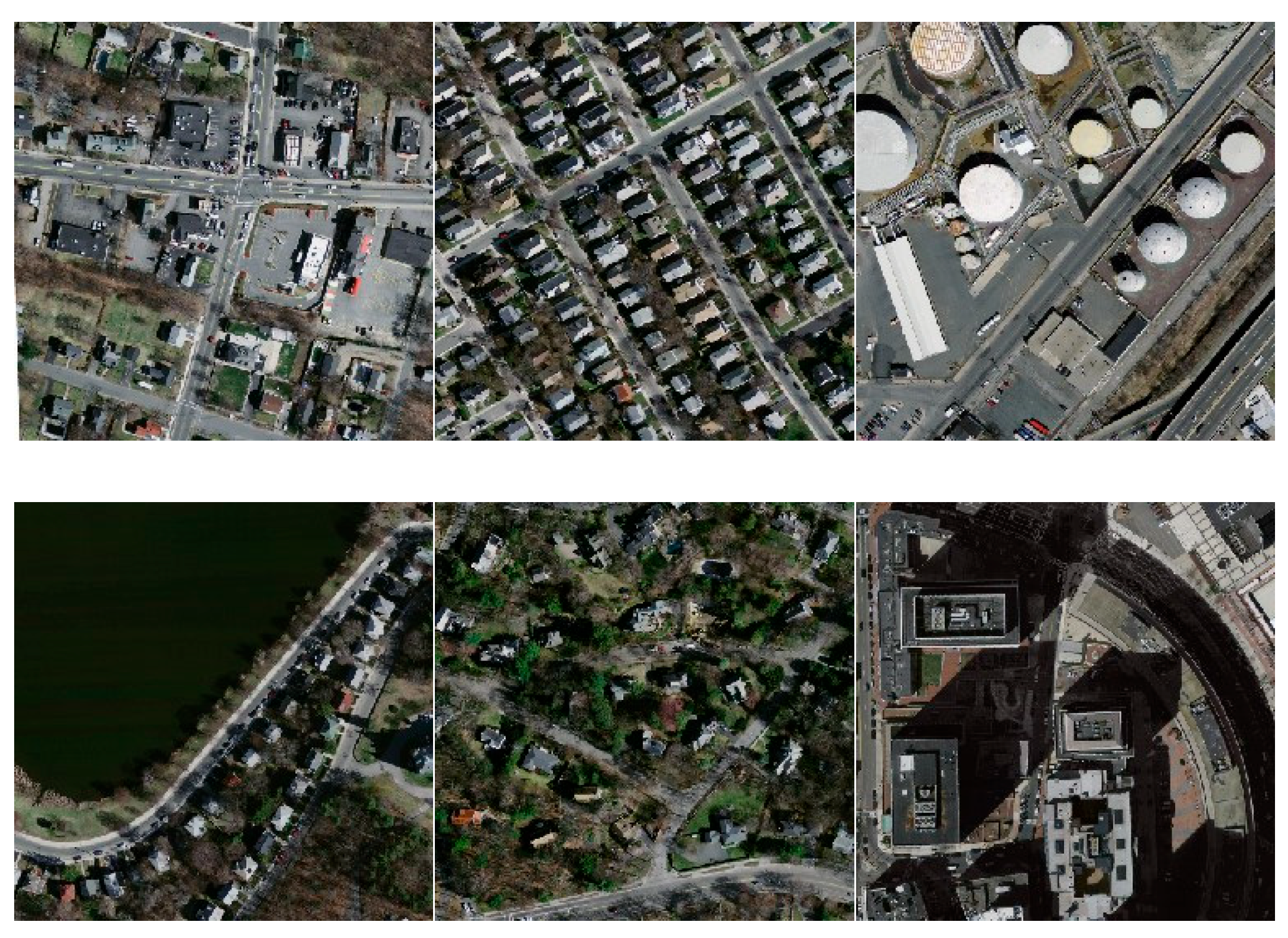
To increase the diversity of the data and improve computational efficiency, the images in the dataset were divided into smaller 256 × 256 pixel patches from the original 1500 × 1500 pixel images. This transformation expanded the dataset from 151 to 3775 images, significantly increasing the variety of building scenes, such as urban buildings along roads, densely arranged small buildings, circular building clusters, lakeside buildings, scattered buildings in dense vegetation, and large buildings under extensive shadows. The images of different scenarios are shown in Figure 5. In the experiment, the dataset was randomly split into training, testing, and validation sets in a specific ratio, with 3075 images used for training, 350 images for testing, and 350 images for validation.

3.3. Data Augmentation

This study employs data augmentation techniques to expand the dataset and address the issue of increased parameters and overfitting as the segmentation model deepens. These methods help improve the model’s generalization performance. As shown in

Table 5. The parameters of different data augmentation.

Augmentation Method	Parameter
Translation	$\pm 15\mathrm{\%}$
Random Rotation	$\pm 15°$
Random Horizontal Flip	$50\mathrm{\%}$
Random Vertical Flip	$50\mathrm{\%}$
HSV Saturation	$\pm 50\mathrm{\%}$

, data augmentation includes operations, such as translation, flipping (horizontal and vertical), rotation, random cropping, and adjustments to the HSV saturation of the existing data samples. Figure 6 illustrates the results after applying data augmentation.

Ablation Study on Augmentation Strategies

To evaluate the contribution of each augmentation technique, we trained REU-Net(2EEAM) on the Massachusetts dataset with only one augmentation enabled at a time. The baseline model (no augmentation) achieved an MIoU of 0.6820, while enabling individual augmentations improved performance as shown in

Table 6. Impact of individual augmentation techniques on model performance (MIoU).

Augmentation Method	$\mathbf{MIoU}$	$∆$
Baseline (No Augmentation)	0.6820	—
+Horizontal Flip	0.7235	+0.0415
+Vertical Flip	0.7157	+0.0337
+Rotation (±15°)	0.7314	+0.0494
+Translation (±15%)	0.7082	+0.0262
+HSV Saturation Adjustment	0.7355	+0.0535
All Combined	0.7952	+0.1132

. Combining all augmentations yielded the highest MIoU of 0.7952, demonstrating their synergistic effect.

The ablation study reveals that each individual data augmentation method provides only limited improvement to the model’s training performance. However, applying all five methods collectively enhances the model’s MIoU by 0.1132. Therefore, in this study, all five augmentation techniques were applied to the dataset, expanding it to 22,650 images, which sufficiently meets the requirements for model training.

3.4. Evaluation Metrics

To comprehensively evaluate the performance of the segmentation network, we employed four widely used evaluation metrics for the semantic segmentation of remote sensing building images in the experiment. These metrics are Precision (P), Mean Pixel Accuracy (MPA), Mean Intersection over Union (MIoU), and Frequency Weighted Intersection over Union (FWIoU). Their definitions are as follows:

$$\mathrm{P}={\displaystyle \frac{\mathrm{BB}}{\mathrm{BB}+\mathrm{NB}}}$$

(14)

$$\mathrm{MPA}={\displaystyle \frac{\frac{\mathrm{BB}}{\mathrm{BB}+\mathrm{NB} }+\frac{\mathrm{NN}}{\mathrm{NN}+\mathrm{BN}}}{2}}$$

(15)

$$\mathrm{MIoU} ={\displaystyle \frac{\frac{\mathrm{BB}}{\mathrm{BB}+\mathrm{BN}+\mathrm{NB}}+\frac{\mathrm{NN}}{\mathrm{NN}+\mathrm{BN}+\mathrm{NB}}}{2}}$$

(16)

$$\mathrm{FWIoU} ={\displaystyle \frac{\mathrm{BB}+\mathrm{BN}}{\mathrm{BB}+\mathrm{BN}+\mathrm{NB}+\mathrm{NN}}}·({\displaystyle \frac{\mathrm{BB}}{\mathrm{BB}+\mathrm{BN}+\mathrm{NB}}})+{\displaystyle \frac{\mathrm{NN}+\mathrm{NB}}{\mathrm{BB}+\mathrm{BN}+\mathrm{NB}+\mathrm{NN}}}·\left({\displaystyle \frac{\mathrm{NN}}{\mathrm{NN}+\mathrm{BN}+\mathrm{NB}}}\right)$$

(17)

In the above formulas, BB represents the number of pixels correctly predicted as building targets; BN denotes the number of pixels incorrectly detected as background targets; NB refers to the number of pixels incorrectly detected as building targets; and NN represents the number of pixels correctly detected as background targets.

In advance, to evaluate the building edge detection capabilities of each model, this paper introduces two evaluation metrics (border IoU and Hausdorff distance), which are defined as shown in the following equations.

$$\mathrm{border} \mathrm{IoU}={\displaystyle \frac{\mathrm{BB}}{\mathrm{BB}+\mathrm{BN}+\mathrm{NB}}}$$

(18)

$$\mathrm{H}\mathrm{D}(\mathrm{A},\mathrm{B}) = \mathrm{m}\mathrm{a}\mathrm{x}({\sup }_{\mathrm{a}\in \mathrm{A}}{\inf }_{\mathrm{b}\in \mathrm{B}}\mathrm{d}\left(\mathrm{a},\mathrm{b}\right),{\sup }_{\mathrm{b}\in \mathrm{B}}{\inf }_{\mathrm{a}\in \mathrm{A}}\mathrm{d}\left(\mathrm{a},\mathrm{b}\right))$$

(19)

where $\mathrm{A}$ and $\mathrm{B}$ represent the sets of predicted and ground truth edge points, respectively, and $\mathrm{d}$ denotes the Euclidean distance.

3.5. Parameter Experiments

We adopted a neural network architecture, REU-UNet(2EEAM), which integrates two EEAM modules, and performed image segmentation on the Massachusetts dataset to determine the optimal weight values for the loss function. To assess the impact of different weight distributions on model performance, we experimented with six parameter combinations (α, β): (0, 1), (0.2, 0.8), (0.4, 0.6), (0.6, 0.4), (0.8, 0.2), and (1, 0), where $\mathsf{\alpha }$ is the weight for the Edge-Consistency Loss (${\mathrm{Loss}}_{\mathrm{EC}}$) and $\mathsf{\beta }$ is the weight for the BCE Loss (${\mathrm{Loss}}_{\mathrm{BCE}}$). The segmentation results are shown in

Table 7. Result of parameter experiments.

REU-UNet(2EEAM)	$\mathbf{P}$	$\mathbf{MPA}$	$\mathbf{MIoU}$	$\mathbf{FWIoU}$
$\mathsf{\alpha }=0$, $\mathsf{\beta }=1$	0.8316	0.5447	0.4642	0.7146
$\mathsf{\alpha }=$0.2, $\mathsf{\beta }=0.8$	0.8032	0.5129	0.4165	0.6552
$\mathsf{\alpha }=$0.4, $\mathsf{\beta }=0.6$	0.8138	0.5366	0.4589	0.6725
$\mathsf{\alpha }=$0.6, $\mathsf{\beta }=0.4$	0.9408	0.8641	0.7952	0.8897
$\mathsf{\alpha }=$0.8, $\mathsf{\beta }=0.2$	0.8365	0.5621	0.4768	0.7043
$\mathsf{\alpha }=$1, $\mathsf{\beta }=0$	0.8039	0.6216	0.5585	0.7884

.

When $\mathsf{\alpha }$ is set to 0.6 and $\mathsf{\beta }$ to 0.4, the segmentation results show significant advantages in terms of P, MPA, MIoU, and FWIoU compared to other networks. Therefore, we set $\mathsf{\alpha }$ to 0.4 and $\mathsf{\beta }$ to 0.6 in the total loss function (${\mathrm{Loss}}_{\mathrm{total}}$).

We conducted an ablation study to compare the proposed hybrid loss (BCE + EC) with other common losses. As shown in

Table 8. Ablation study on loss functions (MIoU, Border IoU).

Loss Function	$\mathbf{MIoU}$	$\mathbf{Border} \mathbf{IoU}$	Training Stability
BCE Only	0.7282	0.7366	High
Dice Loss	0.7524	0.7693	Moderate
Focal Loss	0.7415	0.7583	Low
BCE + Dice	0.7637	0.7912	High
BCE + EC (Proposed)	0.7952	0.9295	High
BCE + EC + Dice	0.7863	0.9016	Moderate

.

It can be found that Dice Loss improves over pure BCE (MIoU: 0.7524 vs. 0.7282) but underperforms BCE + EC due to its focus on regional overlap rather than edge precision. Focal Loss struggles with training stability (fluctuating loss curves) and achieves lower Border IoU (0.7583), likely because it prioritizes hard examples but neglects edge consistency. BCE + EC + Dice shows marginal improvement over BCE + EC but introduces higher complexity. The proposed BCE + EC strikes the optimal balance between edge accuracy (Border IoU: 0.9295) and simplicity.

3.6. Ablation Experiment

In deep learning, ablation studies are an important research method used to better understand network behavior by removing certain parts of the neural network. Robert Long [25] defines ablation studies as the process of removing parts of a complex neural network and testing its performance to gain deeper insight into the network’s internal mechanisms.

In this section, to determine the optimal network configuration that integrates the attention module for achieving the best performance, we conducted four ablation experiments. Specifically, we compared the segmentation performance of networks with no attention module, and networks with one, two, three, or four EEAM attention modules (i.e., REU-Net, REU-Net(1EEAM), REU-Net(2EEAM), REU-Net(3EEAM), and REU-Net(4EEAM)). The evaluation metrics include the loss values during training and the model’s performance on the Massachusetts dataset (P, MPA, MIoU, and FWIoU) to identify the model with the best overall performance for further comparison experiments.

The data analysis in

Table 9. Ablation experiment quantitative comparison of remote sensing building image segmentation results.

Method	$\mathbf{P}$	$\mathbf{MPA}$	$\mathbf{MIoU}$	$\mathbf{FWIoU}$	$\mathbf{Border} \mathbf{IoU}$	$\mathbf{HD}$	Parameters (M)	FLOPs (G)
REU-Net	0.9267	0.8318	0.7632	0.8725	0.7937	5.3994	34.5	65.2
REU-Net(1EEAM)	0.7958	0.7937	0.7116	0.8315	0.8634	3.8762	35.0	67.8
REU-Net(2EEAM)	0.9408	0.8641	0.7952	0.8897	0.9295	1.0893	35.6	69.3
REU-Net(3EEAM)	0.7431	0.8002	0.7214	0.8376	0.8265	3.4238	36.3	72.5
REU-Net(4EEAM)	0.7853	0.7940	0.7080	0.8453	0.8839	1.9930	37.1	75.9

shows that the proposed REU-Net(2EEAM) demonstrates a significant advantage in network configuration: it outperforms other configurations in terms of metrics, such as P, MPA, MIoU, FWIoU, border IoU, HD, Parameters, FLOPs (the forward computation cost for a single image).

Notably, REU-Net(2EEAM) achieves the highest MIoU (0.7952) and Border IoU (0.9295) with a moderate increase in parameters (35.6 M vs. 34.5 M) and FLOPs (69.3 G vs. 65.2 G). In contrast, the result of 1EEAM shows Insufficient edge enhancement due to limited receptive field coverage, and 3/4EEAM’s results show that Excessive modules introduce redundant computations and over-smooth features, degrading performance (MIoU drops by 7.4% and 8.7%, respectively).

Thus, 2EEAM optimally leverages the trade-off between accuracy and complexity by enhancing critical edge features while avoiding over-parameterization.

To highlight that EEAM enhances edge extraction capabilities and improves the overall accuracy of building segmentation by the model, this paper compares REU-Net(2EEAM) with versions where 2EEAM is replaced by three different attention mechanisms: SE-Net, CBAM, and Transformer.

As clearly shown in

Table 10. Performance comparison of models under different attention mechanisms.

Method	$\mathbf{P}$	$\mathbf{MPA}$	$\mathbf{MIoU}$	$\mathbf{FWIoU}$	$\mathbf{Border} \mathbf{IoU}$	$\mathbf{HD}$
REU-Net(SE-Net)	0.7781	0.8129	0.7375	0.8260	0.7264	8.3284
REU-Net(CBAM)	0.7864	0.8315	0.7409	0.8488	0.7583	7.8565
REU-Net(Transformer)	0.8027	0.8374	0.7638	0.8453	0.8471	5.4759
REU-Net(2EEAM)	0.9408	0.8641	0.7952	0.8897	0.9495	1.0893

, REU-Net with 2EEAM outperforms other attention mechanisms in all metrics, demonstrating that 2EEAM significantly contributes to enhancing the model’s segmentation capabilities.

3.7. Comparative Experiments

To evaluate the effectiveness of the proposed improved network REU-UNet(2EEAM), we first selected several classic network models, including FCN8s [15], SegNet [24], BiSeNet [26], DANet [27], PSPNet [28], UNet [16], DeepLabV3+ [29], UNet++ [17], MAFF-HRNet [30], and NPSFF-Net [31], as well as the REU-Net network without the edge-enhancement attention module for building image segmentation experiments. The results were then compared with those of REU-Net(2EEAM) to systematically validate the improvements in segmentation performance. This comparison aims to systematically validate the performance improvement of the modified network in terms of segmentation accuracy.

Table 11. Comparative experiments quantitative comparison of remote sensing building image segmentation results.

Method	$\mathbf{P}$	$\mathbf{MPA}$	$\mathbf{MIoU}$	$\mathbf{FWIoU}$	$\mathbf{Border} \mathbf{IoU}$	$\mathbf{HD}$
FCN8s	0.7404	0.5629	0.3337	0.5085	0.4923	12.8472
SegNet	0.7345	0.5528	0.4166	0.6781	0.5894	10.2834
BiSeNet	0.7372	0.5575	0.4606	0.6546	0.5749	10.3762
DANet	0.7824	0.6860	0.6128	0.7147	0.6022	10.1485
PSPNet	0.8656	0.7763	0.7008	0.8241	0.6793	9.8376
UNet	0.8803	0.8113	0.7276	0.8378	0.7363	8.3764
DeepLabV3+	0.8958	0.8130	0.7223	0.8340	0.7409	8.7465
Unet++	0.8995	0.8035	0.7281	0.8535	0.7781	7.8547
MAFF-HRNet	0.9143	0.7939	0.7639	0.8854	0.7957	7.2376
NPSFF-Net	0.9209	0.8024	0.7655	0.8799	0.8173	6.9487
REU-Net	0.9267	0.8318	0.7632	0.8725	0.8241	6.7364
REU-Net(2EEAM)	0.9408	0.8641	0.7952	0.8897	0.9295	1.0893

presents a quantitative comparison of REU-Net(2EEAM) with other classic networks in the building image segmentation task. The experimental results show that traditional networks like FCN8s, SegNet, BiSeNet, and DANet perform poorly in segmentation accuracy metrics. Although PSPNet, UNet, and DeepLabV3+ show some improvements, they still fall short of UNet++. Further observation reveals that MAFF-HRNet, NPSFF-Net, REU-Net, and REU-Net(2EEAM) show more significant progress in segmentation accuracy. Specifically, REU-Net(2EEAM) achieved the best results in key evaluation metrics, such as P, MPA, MIoU, FWIoU, border IoU and HD, with improvements of 0.9408, 0.8641, 0.7952, 0.8897, 0.9295, and 1.0893, respectively, compared to the baseline UNet model. These results strongly demonstrate the superiority of the proposed improved algorithm in terms of accuracy, while also indicating that the implemented network improvement strategy is both reliable and effective.

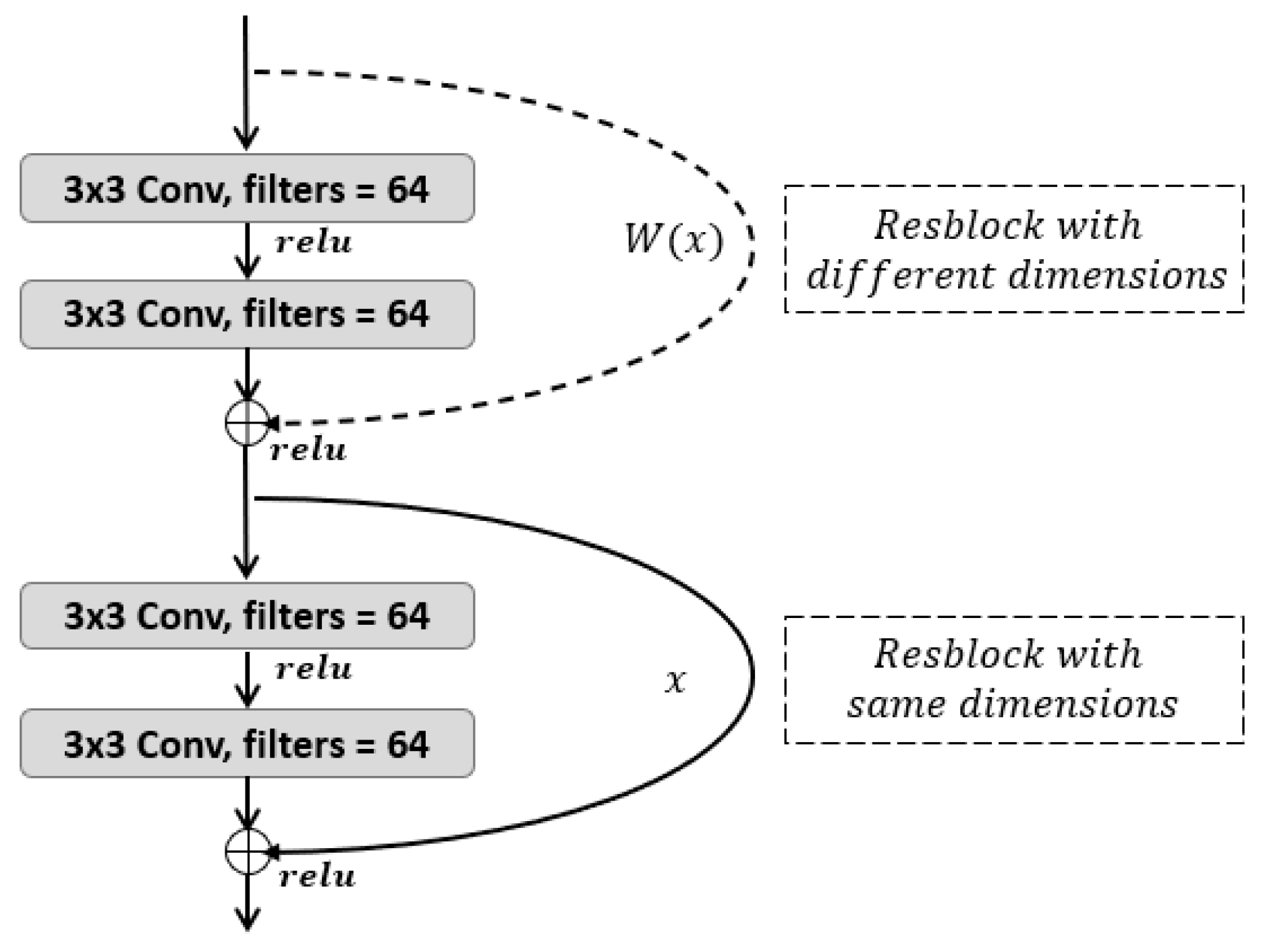
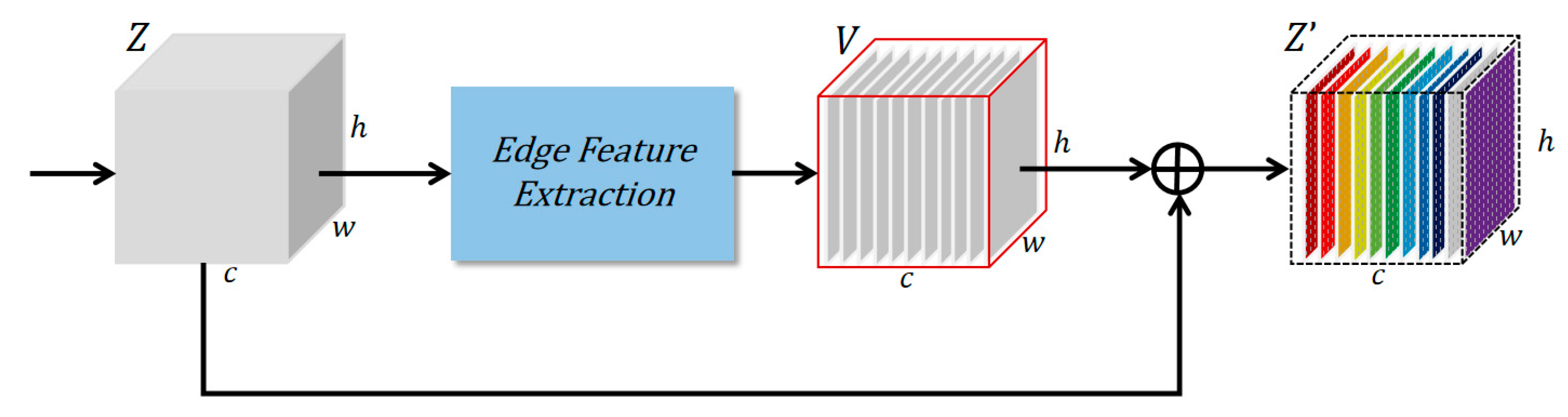
The enhanced segmentation accuracy of REU-Net(2EEAM) compared to other U-Net variants, such as UNet++ or DeepLabV3+, can be attributed to the replacement of traditional 3 × 3 and 1 × 1 convolution blocks with residual blocks (ResBlocks). This modification not only deepens the network architecture but also mitigates the vanishing gradient problem, effectively transferring features from one layer to the next and enabling the extraction of deeper semantic information. Furthermore, direct skip connections are substituted with edge enhancement attention modules. These modules enhance the extraction of building contours and edge information by calculating the difference between positional features and original features, thereby improving segmentation accuracy. Consequently, these improvements enable REU-Net(2EEAM) to achieve superior performance in accurately identifying building edges and enhancing overall segmentation precision.

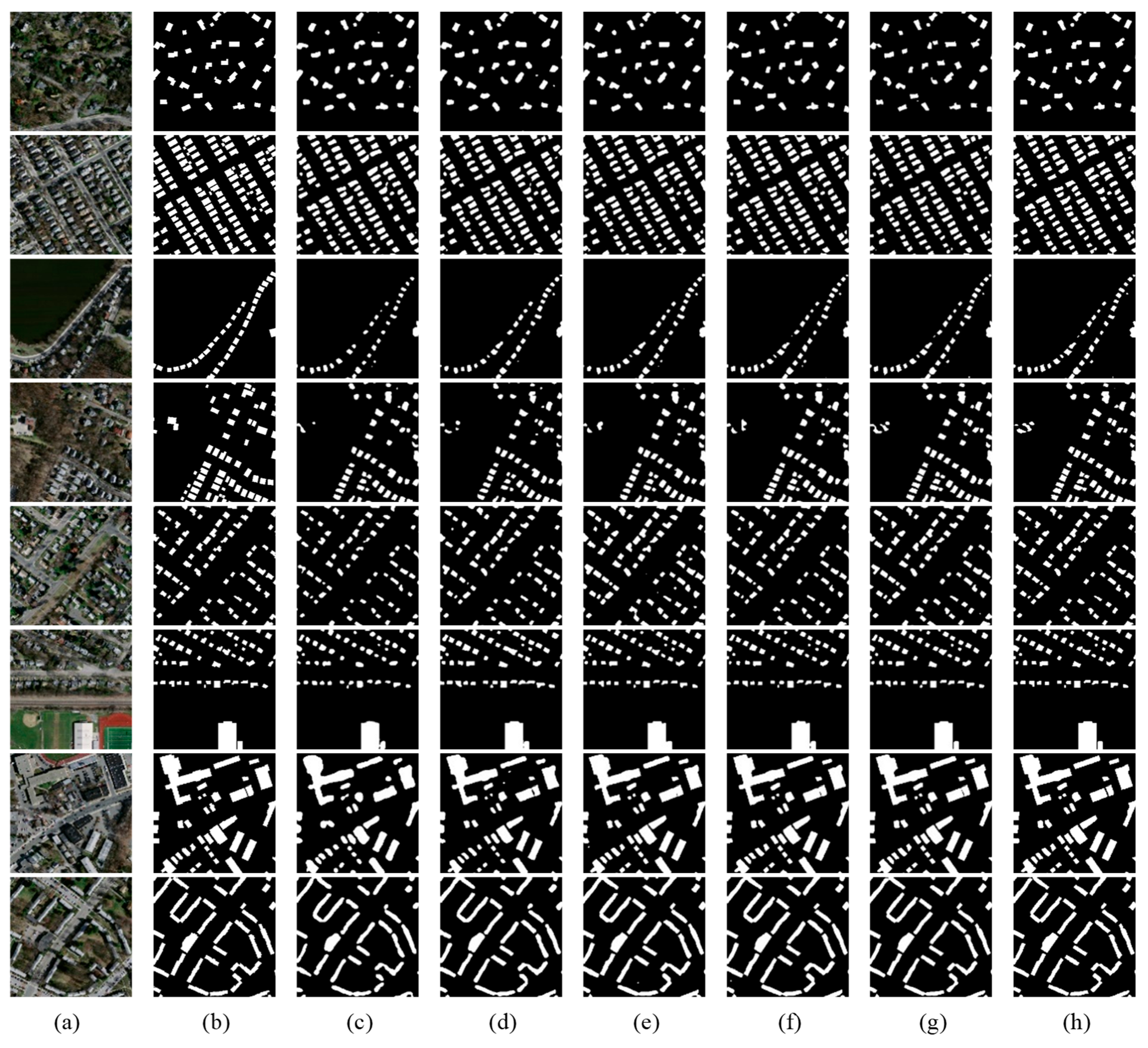
Figure 7 shows that REU-Net(2EEAM) excels in building segmentation tasks across various scenarios. It demonstrates significant advantages, particularly in complex scenarios where buildings are small, sparsely distributed, and overlap with vegetation. In the first, third, and fourth images, the buildings are small and scattered, with vegetation intertwining with the structures, making accurate segmentation more challenging for the model. By incorporating the attention mechanism, REU-Net(2EEAM) enhances its focus on building edge information, allowing it to clearly segment the building outlines and accurately present their shapes. In contrast, other comparison models, lacking the specific handling of edge information, suffer from a significant shape distortion of the buildings and are more sensitive to image noise, leading to the misidentification of non-existent buildings.

In the second and fifth images, which feature dense clusters of small buildings, REU-Net(2EEAM) accurately segments the clear outlines of the buildings and shows a high success rate in identifying smaller structures. Other comparison models, particularly the FCN8s model, fail to effectively capture the edge details of the buildings, resulting in blurry segmentation and a significant distortion of the building shapes.

In the sixth, seventh, and eighth images, which feature mixed scenes of large and small buildings, REU-Net(2EEAM) also performs exceptionally well. Whether accurately capturing the shape of large buildings or recognizing the details of smaller ones, REU-Net(2EEAM) demonstrates its powerful segmentation capabilities. In contrast, other models fail to effectively distinguish between buildings of different scales in complex architectural structures, resulting in imprecise segmentation.

In summary, REU-Net(2EEAM) successfully improves building segmentation accuracy through enhanced edge information, demonstrating superior performance in complex scenarios compared to other models.

In terms of a detailed comparison, as shown in Figure 8, the first image demonstrates that REU-Net(2EEAM) accurately identifies the small building, while REU-Net and UNet, although able to segment the building within the frame, lose varying degrees of detail. PSPNet, BiSeNet, and FCN8s completely fail to segment the building.

In the second image, which contains both a large and a small building, the gap between the two buildings is precisely identified by REU-Net(2EEAM). While REU-Net also recognizes it, the boundaries are somewhat blurred. In contrast, UNet, PSPNet, BiSeNet, and FCN8s fail to fully distinguish the boundaries between the two.

Similarly, in the third and fourth images, REU-Net(2EEAM) accurately identifies the gaps between buildings, while the other comparison models fail to fully distinguish the two buildings. This clearly demonstrates that the introduction of the Edge Enhancement Attention Module significantly improves the accuracy of building segmentation by REU-Net(2EEAM).

To validate the generalization capability of REU-Net(2EEAM), we conducted comparative experiments on three remote sensing datasets: Massachusetts Building Dataset (Dataset 1), WHU Building Dataset (Dataset 2), and Inria Aerial Dataset (Dataset 3). The performance of baseline models (UNet, DeepLabV3+, UNet++), recent state-of-the-art models (NPSFF-Net, REU-Net), and REU-Net(2EEAM) is summarized in

Table 12. Performance comparison across datasets (MIoU and Border IoU).

Method	Dataset 1		Dataset 2		Dataset 3
	$\mathbf{MIoU}$	$\mathbf{Border} \mathbf{IoU}$	$\mathbf{MIoU}$	$\mathbf{Border} \mathbf{IoU}$	$\mathbf{MIoU}$	$\mathbf{Border} \mathbf{IoU}$
UNet	0.7281	0.7363	0.6431	0.6792	0.6103	0.6497
DeepLabV3+	0.7223	0.7409	0.6486	0.6925	0.6593	0.7142
UNet++	0.7281	0.7781	0.7083	0.7496	0.6940	0.7271
NPSFF-Net	0.7655	0.8173	0.7298	0.7736	0.7284	0.7603
REU-Net	0.7632	0.8241	0.7129	0.7583	0.7453	0.8097
REU-Net(2EEAM)	0.7952	0.9295	0.7584	0.8621	0.8294	0.9386

.

As shown in Table 12, REU-Net(2EEAM) achieves the highest MIoU and Border IoU across all datasets, demonstrating robust generalization. For instance, on Dataset 3 (Inria), it outperforms UNet++ by 13.5% in MIoU and 29.1% in Border IoU, highlighting its ability to adapt to diverse building distributions and resolutions.

The significant improvement in Border IoU (e.g., 0.939 on Inria) is attributed to the Edge Enhancement Attention Module (EEAM), which explicitly extracts directional gradients (Sobel operators) and applies spatial weighting to amplify boundary features. This design effectively suppresses background noise while preserving fine-grained edges.

To evaluate whether REU-Net(2EEAM) is suitable for real-time applications, this paper compares the computational costs of several models, including UNet, DeepLabV3+, UNet++, NPSFF-Net, REU-Net, and REU-Net(2EEAM). The computational cost is assessed across the following dimensions.

• Parameters: the number of model parameters (in millions);
• FLOPs: the forward computation cost for a single image (in billions of floating-point operations);
• Inference Time: the inference time for a single image with a batch size of 1 (in milliseconds);
• FPS: Frames Per Second, representing the number of frames processed per second. The calculation formula is as follows: $\mathrm{FPS}=1000/\mathrm{Inference}\mathrm{Time}$.

The experimental results are presented in

Table 13. Computational cost and inference time comparison.

Method	Parameters (M)	FLOPs (G)	Inference Time (ms)	FPS (Batch = 1)
UNet	34.5	65.2	45.3	22.1
DeepLabV3+	41.8	78.9	62.7	15.9
UNet++	36.2	72.1	58.1	17.2
NPSFF-Net	38.4	81.5	68.9	14.5
REU-Net	35.1	68.7	47.5	21.1
REU-Net(2EEAM)	35.6	69.3	48.9	20.5

. For fairness, all inference time measurements were conducted on an NVIDIA RTX 4060Ti GPU with 16 GB of memory. Input images were resized to 256 × 256 pixels, and the batch size was set to 1 to simulate real-time processing scenarios.

As shown in Table 13, REU-Net(2EEAM) achieves a competitive inference time of 48.9 ms per image (20.5 FPS), which meets the real-time threshold (≤100 ms). Compared to UNet++ (58.1 ms) and DeepLabV3+ (62.7 ms), our model reduces inference latency by 15.8% and 22.0%, respectively, while maintaining higher segmentation accuracy (see Table 11). The minor increase in FLOPs (69.3 G vs. UNet’s 65.2 G) is attributed to the EEAM’s edge-enhancement operations, but its parameter-efficient design (35.6 M parameters) ensures compatibility with resource-constrained devices.

4. Conclusions

The proposed REU-Net(2EEAM) network demonstrates significant advantages in the high-resolution remote sensing image building segmentation task, especially in complex scenarios, where it can effectively distinguish the boundaries between buildings, background, and vegetation. By incorporating the Residual Structure, Edge Enhancement Attention Module, and optimizing the network with a hybrid loss combining edge consistency loss and BCE loss, the model can focus more on building edge information, thus improving segmentation accuracy. Compared to other classical networks, REU-Net(2EEAM) exhibits better robustness and segmentation capability in various scenarios, particularly when buildings are small, sparsely distributed, and overlap with vegetation. Additionally, the ablation experiment results validate the significant performance improvement brought by the edge enhancement attention module. Overall, the proposed improved algorithm has strong practicality and broad application prospects, providing new ideas and methods for building segmentation research in the field of remote sensing images.

5. Limitations and Future Work

Despite the promising performance of REU-Net(2EEAM), several limitations should be acknowledged:

• The model struggles to segment buildings smaller than 10 pixels (e.g., isolated huts in rural areas), as shallow features may be lost during downsampling;
• Performance degrades when applied to scenarios with significantly different building styles (e.g., high-density urban vs. sparse villages);
• Processing 512 × 512 images requires 4× more FLOPs than 256 × 256 inputs, limiting real-time deployment on edge devices.

To address these limitations, future work will focus on:

• Enhancing small object detection via adaptive receptive fields;
• Leveraging domain adaptation techniques to reduce data dependency;
• Pruning redundant parameters and exploring knowledge distillation for edge computing.

References

1. Huang, X.; Wen, D.; Li, J.; Qin, R. Multi-level monitoring of subtle urban changes for the megacities of China using high-resolution multi-view satellite imagery. Remote Sens. Environ. 2017, 196, 56–75. [Google Scholar] [CrossRef]
2. Vardanjani, S.M.; Fathi, A.; Moradkhani, K. Grsnet: Gated residual supervision network for pixel-wise building segmentation in remote sensing imagery. Int. J. Remote Sens. 2022, 43, 4872–4887. [Google Scholar] [CrossRef]
3. Feng, W.; Sui, H.; Hua, L.; Xu, C.; Ma, G.; Huang, W. Building extraction from VHR remote sensing imagery by combining an improved deep convolutional encoder-decoder architecture and historical land use vector map. Int. J. Remote Sens. 2020, 41, 6595–6617. [Google Scholar] [CrossRef]
4. Tsu, N. A threshold selection method from gray-level histograms. IEEE Trans. Syst. Man Cybern. 1979, 9, 62–66. [Google Scholar]
5. Andres, T.G.; Gancarski, P.; Berti-Equille, L. Remote sensing image analysis by aggregation of segmentation-classification collaborative agents. Pattern Recogn. 2018, 73, 259–274. [Google Scholar]
6. Wang, M.; Cui, Q.; Wang, J.; Ming, D.; Lv, G. Raft cultivation area extraction from high-resolution remote sensing imagery by fusing multi-scale region-line primitive association features. ISPRS J. Photogramm. Remote Sens. 2017, 123, 104–113. [Google Scholar] [CrossRef]
7. Chen, J.; Li, J.; Pan, D.; Zhu, Q.; Mao, Z. Edge-guided multiscale segmentation of satellite multispectral imagery. IEEE Trans. Geosci. Remote Sens. 2012, 50, 4513–4520. [Google Scholar] [CrossRef]
8. Chen, B.; Qiu, F.; Wu, B.; Du, H. Image segmentation based on constrained spectral variance difference and edge penalty. Remote Sens. 2015, 7, 5980–6004. [Google Scholar] [CrossRef]
9. Lakshmi, S.; Sankaranarayanan, D.V. A study of edge detection techniques for segmentation computing approaches. Int. J. Comput. Appl. 2010, CASCT, 35–41. [Google Scholar] [CrossRef]
10. Zhao, M.; Zhang, X.; Shi, Z.; Li, P.; Li, B. Restoration of motion blurred images based on rich edge region extraction using a gray-level co-occurrence matrix. IEEE Access 2018, 6, 15532–15540. [Google Scholar] [CrossRef]
11. Du, S.; Zhang, F.; Zhang, X. Semantic classification of urban buildings combining VHR image and GIS data: An improved random forest approach. ISPRS J. Photogramm. Remote Sens. 2015, 105, 107–119. [Google Scholar] [CrossRef]
12. Aptoula, E. Remote sensing image retrieval with global morphological texture descriptors. IEEE Trans. Geosci. Remote Sens. 2013, 52, 3023–3034. [Google Scholar] [CrossRef]
13. Mitra, P.; Shankar, B.U.; Pal, S.K. Segmentation of multispectral remote sensing images using active support vector machines. Pattern Recogn. Lett. 2004, 25, 1067–1074. [Google Scholar] [CrossRef]
14. Krizhevsky, A.; Sutskever, I.; Hinton, G.E. ImageNet classification with deep convolutional neural networks. Commun. ACM 2017, 60, 84–90. [Google Scholar] [CrossRef]
15. Long, J.; Shelhamer, E.; Darrell, T. Fully convolutional networks for semantic segmentation. In Proceedings of the 2015 IEEE Conference on Computer Vision and Pattern Recognition (CVPR), Boston, MA, USA, 7–12 June 2015; IEEE: Piscataway, NJ, USA, 2015; pp. 3431–3440. [Google Scholar]
16. Ronneberger, O.; Fischer, P.; Brox, T. U-Net: Convolutional Networks for Biomedical Image Segmentation. In Medical Image Computing and Computer-Assisted Intervention—MICCAI 2015; Springer: Cham, Switzerland, 2015; pp. 234–241. [Google Scholar]
17. Zhou, Z.; Rahman Siddiquee, M.M.; Tajbakhsh, N.; Liang, J. UNet++: A Nested U-Net Architecture for Medical Image Segmentation. In Deep Learning in Medical Image Analysis and Multimodal Learning for Clinical Decision Support; Springer: Cham, Switzerland, 2018; pp. 3–11. [Google Scholar]
18. Tang, P.; Liang, Q.; Yan, X.; Xiang, S.; Sun, W.; Zhang, D.; Coppola, G. Efficient skin lesion segmentation using separable-Unet with stochastic weight averaging. Comput. Methods Programs Biomed. 2019, 178, 289–301. [Google Scholar] [CrossRef]
19. He, N.J.; Fang, L.Y.; Plaza, A. Hybrid first and second order attention Unet for building segmentation in remote sensing images. Sci. China Inf. Sci. 2020, 63, 1–12. [Google Scholar] [CrossRef]
20. He, K.; Zhang, X.; Ren, S.; Sun, J. Deep residual learning for image recognition. In Proceedings of the 2016 IEEE Conference on Computer Vision and Pattern Recognition (CVPR), Las Vegas, NV, USA, 7–12 June 2016; IEEE: Piscataway, NJ, USA, 2016; pp. 770–778. [Google Scholar]
21. Mnih, V.; Heess, N.; Graves, A. Recurrent models of visual attention. arXiv 2014, arXiv:1406.6247. [Google Scholar] [CrossRef]
22. Vaswani, A.; Shazeer, N.; Parmar, N.; Uszkoreit, J.; Jones, L.; Gomez, A.N.; Kaiser, Ł.; Polosukhin, I. Attention is all you need. In Proceedings of the Advances in Neural Information Processing Systems, Long Beach, CA, USA, 4–9 December 2017; pp. 6000–6010. [Google Scholar]
23. Park, T.; Liu, M.-Y.; Wang, T.-C.; Zhu, J.-Y. Edge-aware image synthesis with edge-consistency loss. In Proceedings of the IEEE/CVF International Conference on Computer Vision (ICCV), Seoul, Republic of Korea, 27 October–2 November 2019; pp. 2462–2471. [Google Scholar]
24. Badrinarayanan, V.; Kendall, A.; Cipolla, R. SegNet: A Deep Convolutional Encoder-Decoder Architecture for Image Segmentation. IEEE Trans. Pattern Anal. Mach. Intell. 2017, 39, 2481–2495. [Google Scholar] [CrossRef]
25. Walsh, T.; McClellan, J.M.; McCarthy, S.E.; Addington, A.M.; Pierce, S.B.; Cooper, G.M.; Nord, A.S.; Kusenda, M.; Malhotra, D.; Bhandari, A.; et al. Rare structural variants disrupt multiple genes in neurodevelopmental pathways in schizophrenia. Science 2008, 320, 539–543. [Google Scholar] [CrossRef]
26. Yu, C.; Wang, J.; Peng, C.; Tian, Z.; Yu, D.; Feng, J. BiSeNet: Bilateral segmentation network for real-time semantic segmentation. In Proceedings of the IEEE/CVF Conference on Computer Vision and Pattern Recognition (CVPR), Salt Lake City, UT, USA, 18–22 June 2018; pp. 3201–3210. [Google Scholar]
27. Fu, J.; Liu, J.; Tian, H.; Li, Y.; Bao, Y.; Fang, Z.; Lu, H. Dual attention network for scene segmentation. In Proceedings of the IEEE/CVF Conference on Computer Vision and Pattern Recognition (CVPR), Long Beach, CA, USA, 16–17 June 2019; pp. 3146–3154. [Google Scholar]
28. Zhao, H.; Shi, J.; Qi, X.; Wang, X.; Jia, J. Pyramid scene parsing network. In Proceedings of the IEEE Conference on Computer Vision and Pattern Recognition (CVPR), Honolulu, HI, USA, 21–26 July 2017; pp. 2881–2890. [Google Scholar]
29. Chen, L.-C.; Zhu, Y.; Papandreou, G.; Schroff, F.; Adam, H. Encoder-decoder with atrous separable convolution for semantic image segmentation. In Proceedings of the European Conference on Computer Vision (ECCV), Munich, Germany, 8–14 September 2018; pp. 801–818. [Google Scholar]
30. Che, Z.; Shen, L.; Huo, L.; Hu, C.; Wang, Y.; Lu, Y.; Bi, F. MAFF-HRNet: Multi-Attention Feature Fusion HRNet for Building Segmentation in Remote Sensing Images. Remote Sens. 2023, 15, 1382. [Google Scholar] [CrossRef]
31. Guo, N.; Jiang, M.; Hu, X.; Su, Z.; Zhang, W.; Li, R.; Luo, J. NPSFF-Net: Enhanced Building Segmentation in Remote Sensing Images via Novel Pseudo-Siamese Feature Fusion. Remote Sens. 2024, 16, 3266. [Google Scholar] [CrossRef]
Figure 1. Structure of REU-Net.
Applsci 15 03206 g001
Figure 2. Residual structure.
Applsci 15 03206 g002
Figure 3. Edge feature extraction. (The black arrows indicate the direction of data flow from one layer to another. Transposition (T) indicates the transposition operation used to rearrange the feature maps. Concatenation (C) represents the concatenation of feature maps. Split (S) shows where the feature maps are split for further processing).
Applsci 15 03206 g003
Figure 4. Edge enhancement attention module.
Applsci 15 03206 g004
Figure 5. Diversified data set.
Applsci 15 03206 g005
Figure 6. Diagrams of different data augmentation methods.
Applsci 15 03206 g006
Figure 7. Visual comparison of building segmentation results in ablation experiment. (a) Original image; (b) label; (c) FCN8s; (d) BiSeNet; (e) PSPNe; (f) UNet; (g) REU-Net; (h) REU-Net(2EEAM).
Applsci 15 03206 g007
Figure 8. Detailed comparison of building segmentation results in ablation experiment. (a) Original image; (b) FCN8s; (c) BiSeNet; (d) PSPNet; (e) UNet; (f) REU-Net; (g) REU-Net(2EEAM). (Green boxes highlight the proposed model’s improved accuracy in capturing building edges. Red boxes indicate segmentation inaccuracies by other models).
Applsci 15 03206 g008