The Lumped-Parameter Calorimetric Model of an AC Magnetometer Designed to Measure the Heating of Magnetic Nanoparticles

Abstract

The assessment of superparamagnetic nanoparticle heating is crucial for effective hyperthermia. AC magnetometry can be used to determine the specific absorption rate (SAR) of nanoparticles, assuming proper calorimetric calibration. We show that an AC magnetometer developed in our laboratory can be used simultaneously as a calorimeter for calibrating measurements. An electrical circuit with lumped parameters that are equivalent to the non-adiabatic calorimeter and that incorporates the effects of heat flow from the excitation coil, the surrounding environment, and the sample is presented. Quantitative thermal system identification was performed using global optimization, which fitted the temperature measured by the three fiber-optic probes to the simulated temperature transient curves. The identified model was used to estimate the thermal power generated in the measurement sample using a resistor with a controlled current value. The results demonstrate significant error reduction, particularly at lower heating powers, where external heat transfer becomes more influential. At low heating power values (around 25 mW), the error was reduced from 16.09% to 2.36%, with less pronounced improvements at higher power levels. The model achieved an overall accuracy of less than 2.5% across the 20–200 mW calibration range, a substantial improvement over the corrected-slope method. The value of the true thermal power of nanoparticles can be obtained using the calibrated calorimeter.

1. Introduction

Magnetic nanoparticles have been extensively researched due to their potential use in various medical applications, including anti-cancer hyperthermia treatment [1,2], medical imaging [3,4], and theranostics [5,6,7]. The therapeutic effect of hyperthermia is based on increasing the temperature of tumor tissues, typically to around 40–43 °C [8]. In this temperature range, cancerous cells are killed by inducing programmed cell death, which is called apoptosis [9]. The primary goal of nanoparticle application in hyperthermia is to maximize the power deposition inside the tumor’s tissue. The iron mass-normalized specific absorption rate (SAR) is the physical quantity commonly used for evaluating the nanoparticle heating efficiency when subjected to alternating magnetic fields [10]. An accurate determination of SAR is crucial for quantifying the ability of superparamagnetic nanoparticles (SPIONs) to generate heat during AC magnetization [11]. Adiabatic conditions are most preferred for precise SAR measurements [12]. However, experimental analysis in alternating magnetic fields requires a unique calorimeter design composed of nonmagnetic materials, which may not guarantee perfect thermal isolation.

We built a hybrid system for SAR measurement using both AC magnetometry and calorimetry, as presented in [13,14]. The application of an ideal calorimetric model did not achieve acceptable compliance between the two methods. The measured heating curves poorly fit the theoretical adiabatic curves. In such a case, non-adiabatic conditions must be considered to avoid significant errors. Non-ideal calorimeter measurements require extended analysis, in which more specific parameters like the examined sample’s thermal resistance or heat capacity need to be considered to properly model the undesired outward heat flow from the sample to the environment [15].

Several approaches have already been proposed by different authors to describe the non-adiabatic behavior of calorimeters designed for measuring the heating power of ferrofluids. These methods range from simple models based on a single heat loss parameter to more advanced multi-parameter differential equations that account for complex heat loss mechanisms. One of the most widely used models for non-adiabatic conditions is the corrected-slope method [16], which represents heat loss with a single linear parameter. More sophisticated models introduce multiple thermal parameters to more accurately describe the thermal properties of the entire calorimetric system and simultaneously model various heat loss mechanisms, including dissipation effects due to radiative losses [17,18].

Another approach to modeling non-adiabatic calorimeters involves complex and time-consuming numerical simulations using the finite element method (FEM), which allows for a more detailed analysis of thermal behavior. Although computationally demanding, this method enables a more precise assessment of heat dissipation. Researchers have also developed numerical models of nanoparticle heating [19,20] using various experimental setups, such as inside a glass test tube [21] or within small animals [21].

Despite these advancements, the vast majority of studies evaluate their models primarily based on how well the simulated curves fit the experimental data, without explicitly assessing the measurement accuracy of their calibrated systems or comparing their models with others available in the literature.

The non-adiabatic heat flow analysis, which takes place in the calorimeter, may be simplified if the thermal properties of the sample and its surroundings are represented by the lumped elements of the thermoelectric circuit. All the parameter values the model represents must be found via estimation or the calibration process. For example, in [16], the authors indicate that the heat capacity $C$ of the sample may be easily calculated with the given mass m of the sample and its specific heat value $C_s$ according to Formula (1), whilst the thermal resistance requires special estimation algorithms.

$$C=C_{s}m$$

(1)

The heat capacity of other model’s elements of defined mass and specific heat can also be estimated using (1). However, in order to obtain highly accurate, detailed calibration is necessary. This can be achieved using an excitation input signal from a power-controlled heat source.

The analysis of heat flow in non-adiabatic calorimeters with different levels of complexity has been previously proposed and compared in several studies. For instance, a detailed approach to the transient analysis of equivalent circuits for various thermal systems has been presented in [22,23,24]. Multiparameter thermo-electric equivalent circuits have also been used to model heat sinks and thermal sources [25,26], as well as lithium-ion batteries in [27,28,29,30]. Additionally, several authors have developed a nonlinear RC-thermal circuit with variable thermal resistance [31]. Examples of lumped-parameter thermal modeling in various applications can be found in [32,33,34,35,36,37]. In particular, a lumped-element equivalent RC circuit with multisensory simultaneous measurements for the thermal identification of the examined apparatus was proposed in [38]

Thermal modeling using lumped-parameter thermal networks is associated with uncertainty regarding the power loss model and the computational complexity of identifying the model using global optimization. To address these challenges, data-driven nonlinear function approximation using supervised machine learning has been proposed in [39,40].

In this paper, an equivalent thermo-electric circuit (equivalent thermal network) is proposed for a non-adiabatic measurement system designed to perform thermal power measurements of nanoparticles exposed to an alternating magnetic field. In our RC lumped-element model, apart from the parameters included in the simplest non-adiabatic corrected-slope method, such as the heat capacity of the nanoparticle sample and its thermal resistance to the surroundings, we also consider other factors affecting the measurement error, based on findings from other studies. For example, Hanson et al. [41] noted that different levels of insulation in the closest surroundings of the non-adiabatic system lead to varying heating time curves. Therefore, the thermal properties of the sample’s closest environment must be considered in the corrected-slope formula to accurately determine the heating power of the sample. To address this issue, we modeled the thermal resistivity and capacity of the surrounding environment using additional RC lumped elements. A similar model incorporating these parameters into a set of differential equations describing heat flow in the system can be found in [42,43]. One publication [38] presents an approach where the authors used a lumped-element model to describe the sample’s immediate environment, but specifically in a differential calorimeter setup.

In our measurement setup, magnetic nanoparticles were heated by a strong alternating magnetic field generated by a large current flow through the excitation coil. Such a large current driven through the resistive wires of the coil also created heat, resulting in a substantial temperature rise in the carcass and its surroundings. A specially adapted cooling system for the excitation coil was used to reduce this effect significantly. However, if the efficiency of the cooling system is insufficient to drain all of the dissipated energy, some heat may still be transferred to the sample and its surroundings, resulting in an overestimation of the input power [44]. This is particularly important if the nanoparticle heating efficiency is low compared to the external heat flow, just like it was in our case. We extended the lumped equivalent circuit-based thermal model by adding an external power source and two additional resistive elements reflecting the degree of heat transfer from the excitation coil to the sample and its surroundings. To the best of the authors’ knowledge, this aspect has not been addressed in previous publications on modeling non-adiabatic calorimeters for ferrofluid measurements.

In addition to the expansion of the non-adiabatic calorimeter model, we increased the number of temperature curves recorded at three different points of the measurement system, using a total of three independent fiber-optic thermometer probes: two for monitoring the temperature changes at the two nodes of the system corresponding to the sample and its closest surroundings, and an additional one to track the temperature change in the carcass heated by the resistive power loss generated by the induction coil, which caused an undesired temperature increase in the sample and its surroundings. The result was an increased quantity of calibration data for the global optimization system, leading to a more reliable estimation of the multi-parameter RC model. To the authors’ knowledge, the use of multi-probe measurements in a non-adiabatic calorimeter system for ferrofluid heating power measurements has not been encountered in the literature.

We show that this thermal model enables the proper calibration of power measurements using an AC magnetometer. The parameter values of the presented model were identified by a numerical global optimization algorithm that fits temperature-time curves to measurement data. For this procedure, calibration measurements were performed with fiber-optic probes and two adjustable power sources, namely a heating resistor and excitation coil, which were both controlled by the independent DC voltage source. Another approach to the linear calibration of a quasi-adiabatic calorimeter used to perform SAR measurements of nanoparticles using a piece of copper wire was presented in [45]. The authors estimated the power dissipation in the sample by theoretically calculating the eddy currents generated in the thin copper wire subjected to an alternating magnetic field.

A new idea presented in our paper is the use of direct current instead of alternative current in the excitation coil during the calibration. The direct current driven through the excitation coil allowed us to determine the influence of external heating on the examined sample without inducing any excess thermal power from eddy currents in the heating resistor wires.

The calibration results for the proposed expanded model with three-point temperature measurement were compared with the calibration and verification results for the standard model with a single heat loss parameter, corresponding to the corrected-slope method.

2. Materials and Methods

2.1. Magnetic Nanoparticle Heating System

Our laboratory’s hybrid system for nanoparticle heating measurement was described in [13,14]. It allowed for the verification of AC magnetic measurements with calorimetric measurements. The setup for the calorimetric measurement of magnetic nanoparticles is shown in Figure 1a.

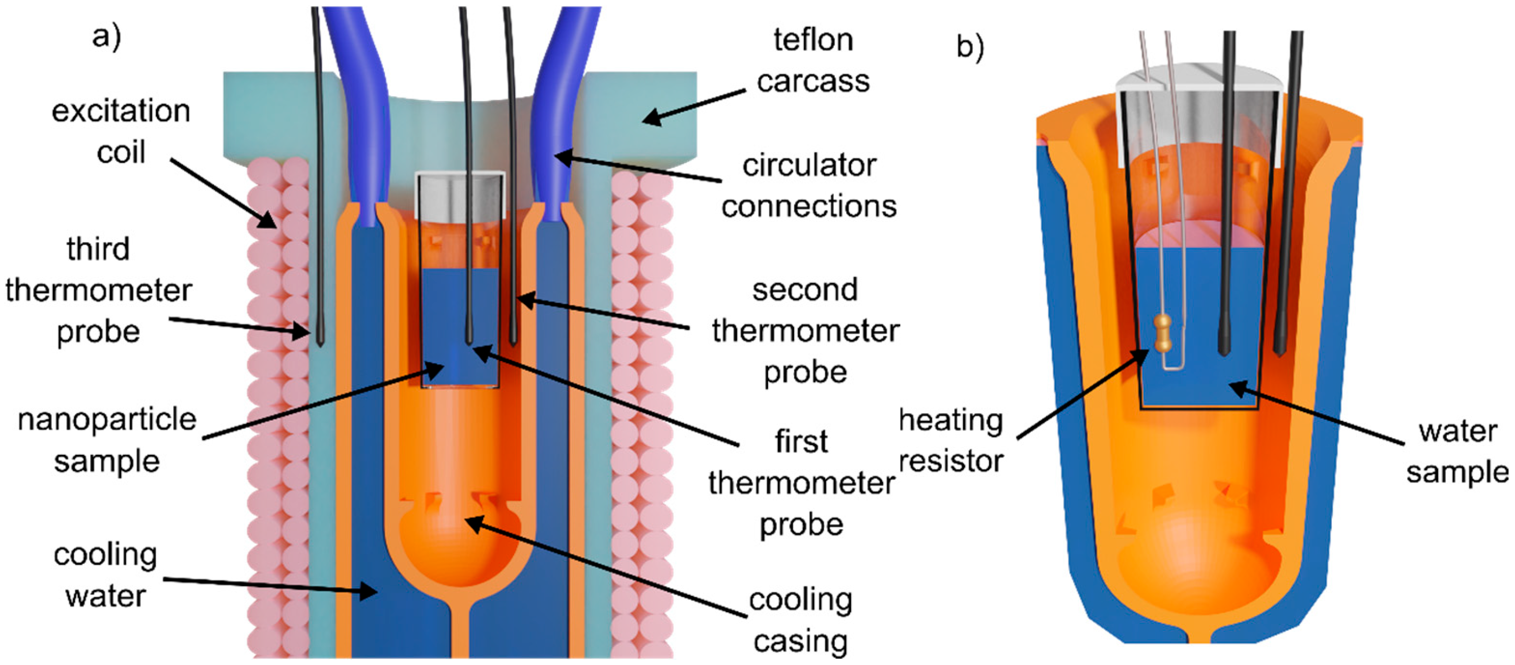
A test tube filled with a nanoparticle solution was placed inside a cooling casing that was 3D printed from acrylonitrile butadiene styrene (ABS). The model was post-processed using acetone vapor polishing to improve the surface smoothness and ensure water-tightness. A ThermoScientific A10 refrigerated circulator (Thermo Fisher Scientific, Waltham, MA USA) forced water flow through the cooling casing, thermally insulating the sample from the resistive heat generated by the excitation coil and ensuring temperature stability. The alternating magnetic field provided by the excitation coil enabled nanoparticle magnetization, leading to energy dissipation in the form of heat. A thermometer with three nonmagnetic fiber optic probes was used to measure temperature changes. The first probe was placed inside the test tube through a tiny hole in the tube’s cap. The second probe was inserted into the airspace between the test tube and the wall of the cooling casing. The third probe was located in a hole drilled in the wall of the polytetrafluoroethylene (PTFE) carcass on which the excitation coil was wound. The system was slightly modified to enable proper calibration. A small hole was also drilled in the cap of the sample for a heating resistor to be placed in the deionized water (Figure 1b).

2.2. Equivalent Thermo-Electrical Circuit

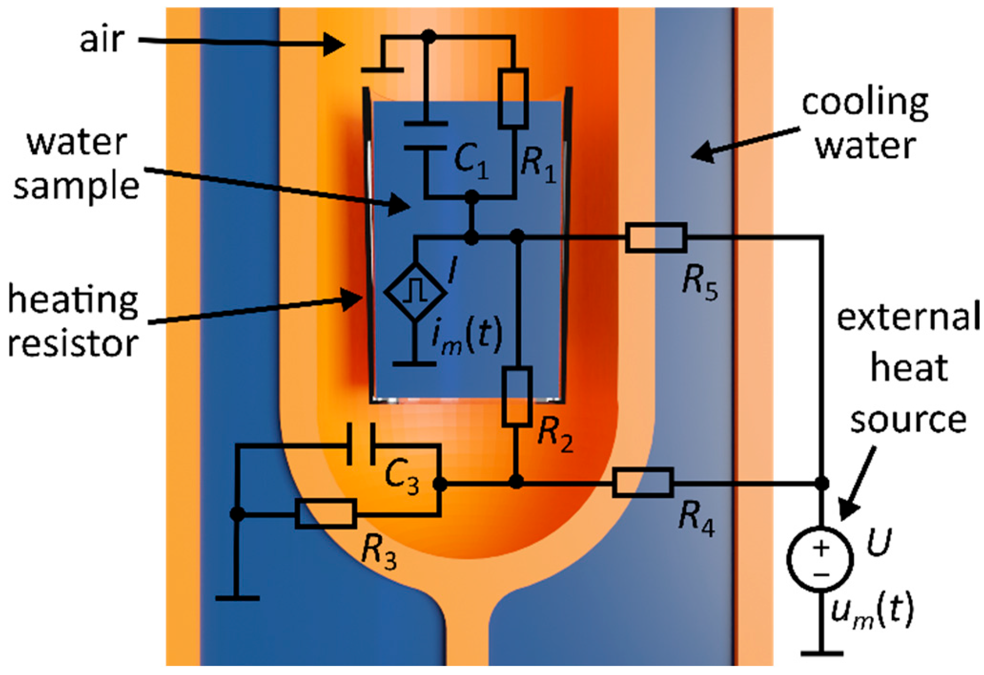
The approximate electrical equivalent circuit of the thermal system with lumped elements is shown in Figure 2. The current source $i_m\left(t\right)$ represents the controlled heat flow source in the form of the SMD 0408 16 kΩ resistor immersed in the water sample. The input thermal power was a rectangular pulse function corresponding to the resistive power dissipated by the heating resistor, with the adjustable amplitude regulated for each of the $m$-th measurements.

The capacitor $C_1$ described the heat capacity of the 2 mL water sample and could be roughly estimated according to Formula (1) as 8.368 J/(g °C). The heat capacity of the calorimeter’s airspace was introduced into the model by $C_2$. $R_1$ characterized the thermal resistance between the water sample and the environment, while $R_2$ corresponded to the thermal resistance between the water sample and the airspace inside the calorimeter. $R_3$ represented the thermal resistance between the calorimeter’s airspace and the environment.

In our project, we used Litz wire for the construction of the induction coil, in contrast to other authors who used copper tube windings cooled by forced water flow inside the tube [46]. The use of Litz wire was particularly advantageous due to the need to reduce the coil’s resistance by mitigating the skin effect at high RF frequencies. The system was cooled using a water jacket with an automatically cooled continuous water circuit, which absorbed heat from the heating carcass of the induction coil while simultaneously maintaining a constant reference temperature in the immediate vicinity of the heated sample. Despite using water cooling, we observed that a small portion of the temperature rise in the sample resulted from the inward heat flow generated by the resistive energy dissipated in the excitation coil. This effect was modeled by adding an external temperature source connected to the calorimeter’s airspace and the sample via thermal resistances $R_4$ and $R_5$, respectively. The transient temperature curve registered by the probe placed inside the excitation coil’s carcass served as an input signal $u_m\left(t\right)$.

A direct current was applied to the coil during the calibration experiments to generate resistive heat. Using an alternating magnetic field in the calibration measurements would have caused the uncontrolled heating of the resistor and wires due to eddy currents, as reported in [42,43]. This problem was eliminated in our experiments by measuring the temperature with nonmagnetic fiber optics sensors and the application of direct current in the excitation coil during the calibration procedure. While DC could not heat the nanoparticles, it allowed us to control the thermal power produced by the excitation coil.

Using a refrigerated circulator, we set the desired controlled temperature to 25 °C, similar to the environment temperature measured during our experiments. This allowed us to assume that the uniform ground potential for the whole model would be 25 °C.

The range of power values selected for calibration was based on the observed temperature increase in the initially tested nanoparticle solutions (OceanNanotech SPA-25, San Diego, CA, USA). With the magnetic fields used, in the order of several mH, a maximum temperature rise of about 10 °C was observed in the nanoparticle solution during the 3600 s measurement, which approximately corresponds to around 200 mW in a lossless, adiabatic system. To balance the calibration time with the accuracy required in determining the model parameters, five different heating resistor power values (0 mW, 14.1 mW, 56.4 mW, 127.0 mW, 225.7 mW) were selected. These corresponded to the voltage values set on the generator (15 V, 30 V, 45 V, 60 V), with 60 V being the highest available setting on the voltage power supply. Given the heating resistor’s resistance of 15,950 Ω, these voltage settings resulted in the corresponding power values. These were combined with the four different power loss values (0 W, 3.3 W, 22.2 W, 59.4 W) generated by the DC current in the excitation coil circuit. The upper limit of the selected range was chosen to match the maximum current available for the excitation coil load at the highest frequency designed for AC magnetometry {12 mH (25 A) at 350 kHz}. The power losses corresponded to different temperature curves recorded at the coil carcass and were subsequently used as the excitation signal for the voltage source $u_m\left(t\right)$. As a result, after discarding the combination that provided no meaningful contribution (0 mW, 0 W), a total of 19 calibration combinations were used.

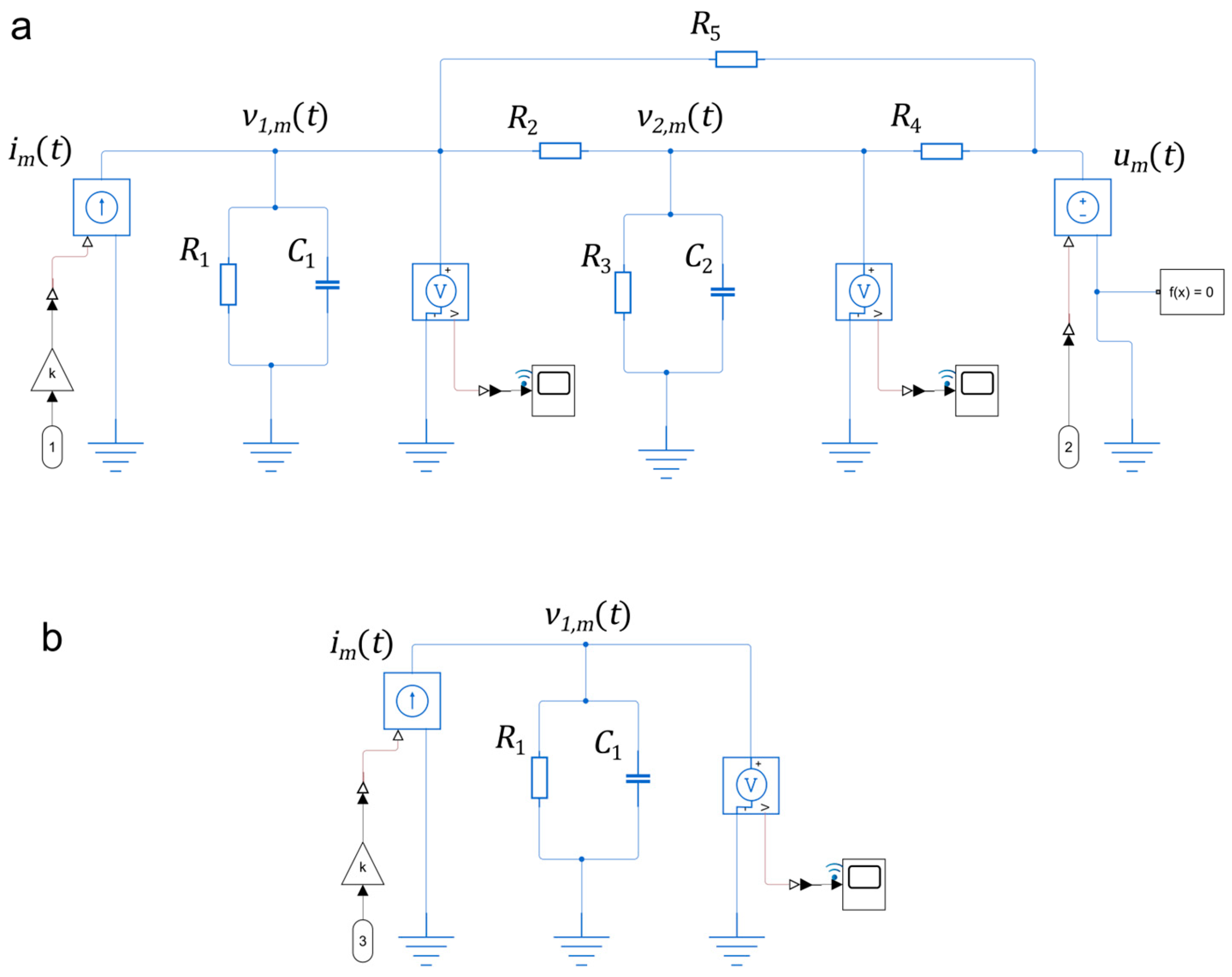
The proposed lumped model circuit (C2R5) and the equivalent lumped model corresponding to the corrected-slope method (C1R1) were created in the Simscape Simulink simulator (Figure 3). The heating resistor is represented by the current source unit pulse function $i_m\left(t\right)$ and its gain k, while the temperature of the inner wall of the coil carcass is described by the continuous function $u_m\left(t\right)$. The input excitation $i_m\left(t\right)$ was a rectangular pulse with a duration of 3600 s, after which it was turned off. Once the pulse ended, the system entered the cooling phase, and the temperature was recorded for an additional 3600 s. Throughout both the heating and cooling phases, $u_m\left(t\right)$ reflected the thermal response of the heated carcass.

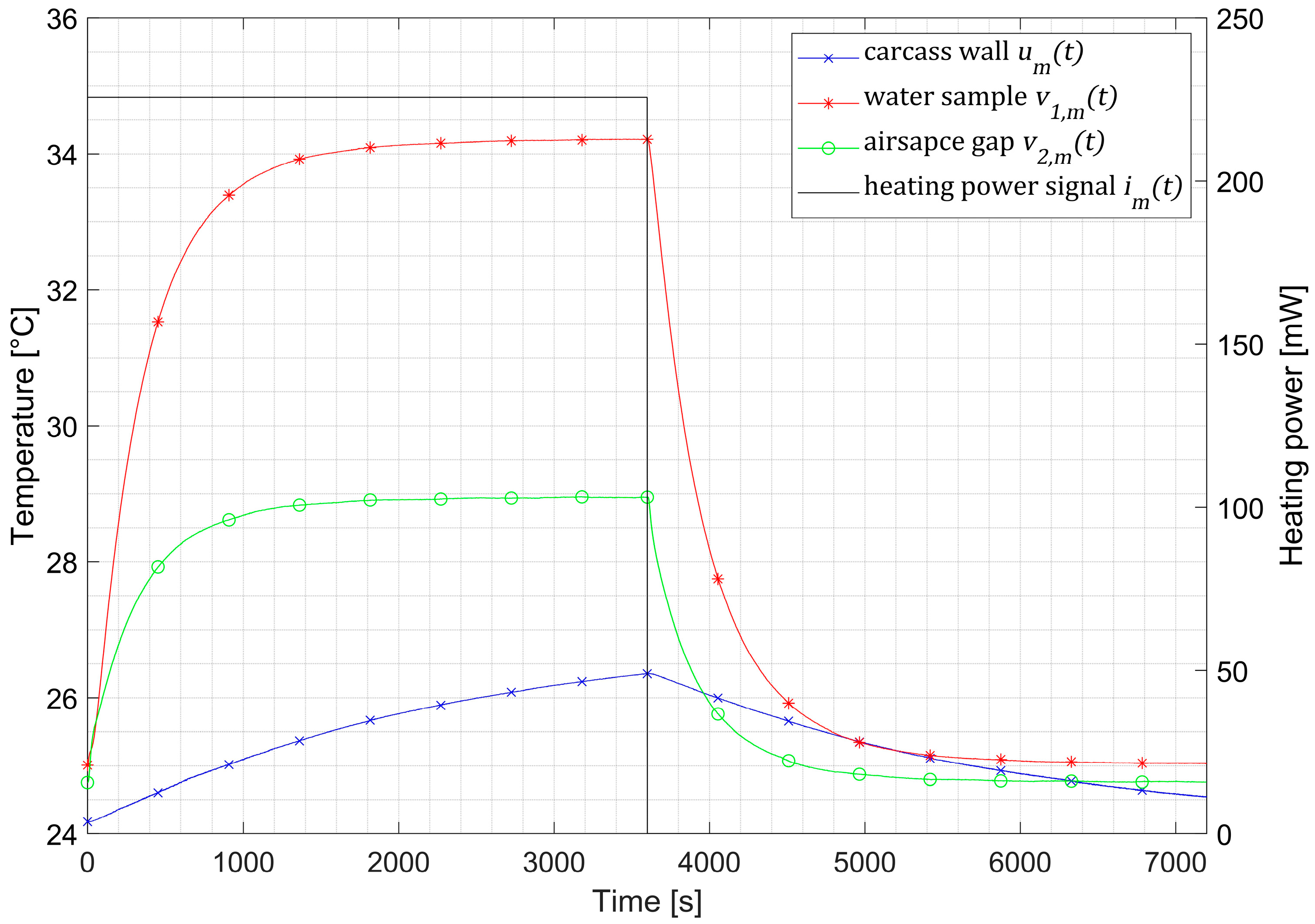
Several measurements were performed to identify the system RC parameters using two Osensa LUX 200+ temperature transmitters (OSENSA Innovations, Burnaby, BC, Canada) and three non-magnetic fiber-optic PRB G-40 probes, sampled at a frequency of 11 samples per second. As previously mentioned, the first probe measured the temperature of the 2 mL sample filled with water. The second and third probes recorded the temperature of the calorimeter’s airspace and the coil carcass, respectively. All temperatures were measured according to the manufacturer’s calibration note, with an accuracy of 0.1 °C and a precision of 0.02 °C. The transient temperature curves (Figure 4), measured by probes 1 and 2, correspond to the Simulink model’s potentials, measured by the voltmeters at two circuit nodes, namely $v_{1,m}\left(t\right)$ and $v_{2,m}\left(t\right)$ (Figure 3). The transient curves of the recorded temperature in the water sample, the airspace inside the calorimeter, and the excitation coil’s carcass, together with the input power pulse of the heating resistor, are presented in Figure 4.

2.3. Identification of Equivalent Electrical Circuit

Let us assume that an electric circuit is described by a nonlinear function f, which maps the excitations at given circuit nodes to the voltage at other nodes. The unknown parameters of this function are the values of lumped elements. The $m$-th time excitation at the $n$-th node can be described by the following equation:

$$v_{n,m}\left(t\right)=f\left(i_m\left(t\right),u_m\left(t\right),R_1,C_1,R_2,R_3,C_3,R_4,R_5\right)$$

(2)

where $i_m\left(t\right)$ is the current function corresponding to the heating power of the resistor-heater, $u_m\left(t\right)$ is the voltage function corresponding to the carcass temperature, $v_{n,m}$ is the voltage at measurement node $n\in \left\{\mathrm{1,2}\right\}$ corresponding to the temperature measured by fiber-optic probes placed inside the sample and its surroundings in measurement $m=1, \dots , 19$; and $R_1$, $C_1$, $R_2$, $R_3$, $C_3$, $R_4$, $R_5$ are the parameters presented in Section 2.2.

As a result, we obtained a nonlinear system of equations with seven unknowns. The measurements were selected to cover the expected thermal power range of the nanoparticle samples (from 0 mW to 225 mW) and the thermal power generated by the active excitation coil (up to 60 W). Five different current levels in the heating resistor and four thermal power levels in the operating excitation coil were used.

The values of the function $f$ were calculated numerically by MATLAB Simscape Toolbox Version 5.4. Due to the complexity of $f$, we could not guarantee that the minimized objective function was concave over its entire domain, meaning that local minima might exist. Therefore, the parametric fitting of the model to the measured data was performed using the surrogate optimization algorithm from the MATLAB Global Optimization Toolbox Version 4.8. The stopping criterion was set to a maximum of 700 iterations.

3. Results

The RC parameters of the proposed lumped model and the model derived from the corrected-slope function were estimated based on the MATLAB Global Optimisation toolbox and measured temperature curves. All the fitted parameters for both models are listed in

Table 1. The parameters of the model.

Element	Symbol	C2R5	C1R1
Thermal capacity of the water sample	$C_1$	$7.60 {\displaystyle \frac{\mathrm{J}}{\mathrm{g}·°\mathrm{C}}}$	$9.32 {\displaystyle \frac{\mathrm{J}}{\mathrm{g}·°\mathrm{C}}}$
Thermal resistance between the water sample and the environment	$R_1$	$44.25 {\displaystyle \frac{°\mathrm{C}}{\mathrm{W}}}$	$44.80 {\displaystyle \frac{°\mathrm{C}}{\mathrm{W}}}$
Thermal resistance between the water sample and the airspace	$R_2$	$1.39 {\displaystyle \frac{°\mathrm{C}}{\mathrm{m}\mathrm{W}}}$	-
Thermal capacity of the calorimeter airspace	$C_3$	$0.05 {\displaystyle \frac{\mathrm{J}}{\mathrm{g}·°\mathrm{C}}}$	-
Thermal resistance between the calorimeter’s airspace and the environment	$R_3$	$1.23 {\displaystyle \frac{°\mathrm{C}}{\mathrm{m}\mathrm{W}}}$	-
Thermal resistance between the external temperature source and the sample	$R_4$	$171.17 {\displaystyle \frac{°\mathrm{C}}{\mathrm{m}\mathrm{W}}}$	-
Thermal resistance between the external temperature source and the calorimeter’s environment	$R_5$	$1.50 {\displaystyle \frac{°\mathrm{C}}{\mathrm{m}\mathrm{W}}}$	-

. The fitted model response and the corresponding temperature curves measured for the same exemplary input power are presented in Figure 5. It is noteworthy that model C1R1 does not account for the heating effect had by the excitation coil on the sample, which, for the case of power losses in the excitation coil of around 60 W, resulted in an increase in the temperature of the sample by approximately 0.35 °C (Figure 5(a2)).

From all the fitted values, the value of $C_1$ could be easily compared to the theoretical thermal capacity of the 2 mL water sample, which, according to Formula (1), equals 8.368 J/(g °C) and differs by up to 12% in each model compared to the theoretical value. This discrepancy could result from the imprecise placement of the thermometer in the center of the sample, as mentioned by several authors before [16,47]. Our calibration protocol could be performed each time a new nanoparticle sample is placed, along with the positioning of all the fiber-optic thermometer probes. After calibration is completed and all probes are fixed in place within the measurement setup, the power resistor is removed from the nanoparticle solution while the positions of the probes remain unchanged, which partially eliminates the positioning error. Therefore, even though the probes’ positions might vary slightly with each measurement, this positioning error is partially compensated during the calibration process, where slightly different capacitance values are fitted instead of using the exact values calculated from the formula. This approach also enables the fitting of capacitance values for a variety of solutions, not limited to water-based ones, but also including more complex solvent mixtures.

The polyamide test tube was precisely filled with deionized water using the automatic pipette. However, it should be noted that although the test tubes were closed tightly, two tiny holes in the cup for the fiber-optic probe and the heating resistor were only partially isolated, allowing for the evaporation of a small amount of water, especially during the long 48 h calibration measurements. Both models were validated for five selected power values that were generated by the heating resistor and a single constant value of thermal power that was generated by the excitation coil. All of the excitations were different from those used for the model identification. The input power values were estimated based on the recorded heating curves and the equivalent lumped thermo-electric model, with the fitted parameter values assigned to the corresponding elements. Rectangular pulses with the same duration as those used in the calibration processes were used as input power functions. The amplitude $k$ of the pulse $i_m$, which corresponds to the excitation power of the heating resistor, was the only parameter estimated in each measurement during the validation phase. Single-parameter fitting was a less complicated problem than the least-square fitting of seven RC parameters conducted in the calibration process. Because of that simplification, a global optimization algorithm was replaced with the least-square linear algorithm, which converged much faster. All the values of the thermal power and the measurement errors are listed in

Table 2. Relative errors of input heating power according to identified lumped-element models.

Power at Excitation Coil [W]	True Input Power Value [mW]	Estimated Input Power Value [mW]		Relative Error [%]
		C2R5	C1R1	C2R5	C1R1
38.05	25.08	25.67	29.11	2.36	16.09
38.05	39.19	39.92	41.59	1.88	6.14
38.05	76.80	76.81	77.72	0.02	1.19
38.05	100.31	100.05	99.60	0.26	0.71
38.05	156.74	154.49	153.54	1.43	2.04
38.05	189.66	186.65	185.60	1.58	2.14

. The relative measurement error was calculated using the following formula:

$$e=\left|{\displaystyle \frac{{P_{true}-P}_{estimated}}{P_{true}}}\right|100\%$$

(3)

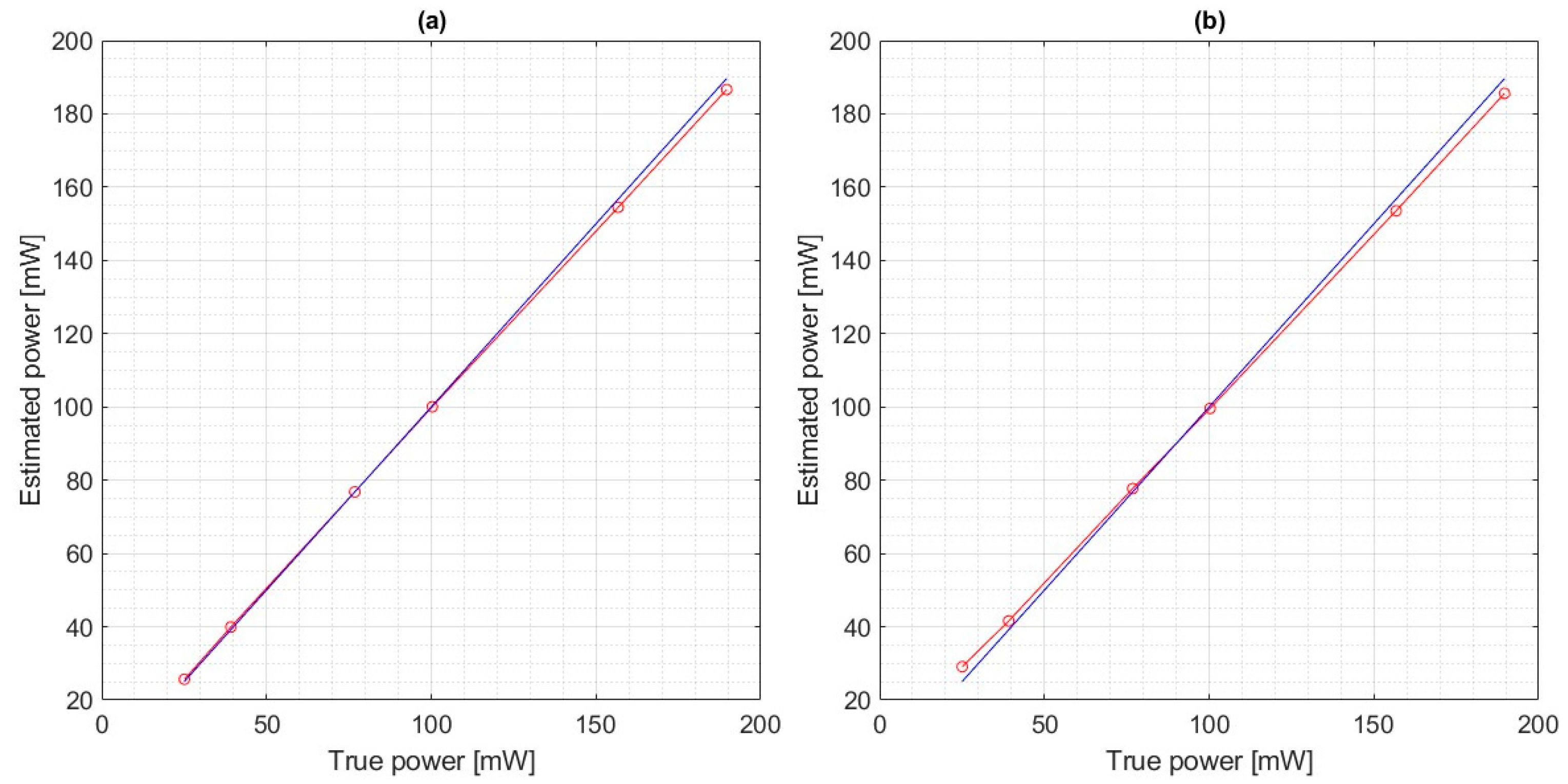
Identifying the equivalent electrical models allowed the calorimeter to be calibrated and used to measure the actual value of the input heating power, even when disturbed by an external heat flow. The estimated power values were plotted as a function of the true power values, as shown in Figure 6.

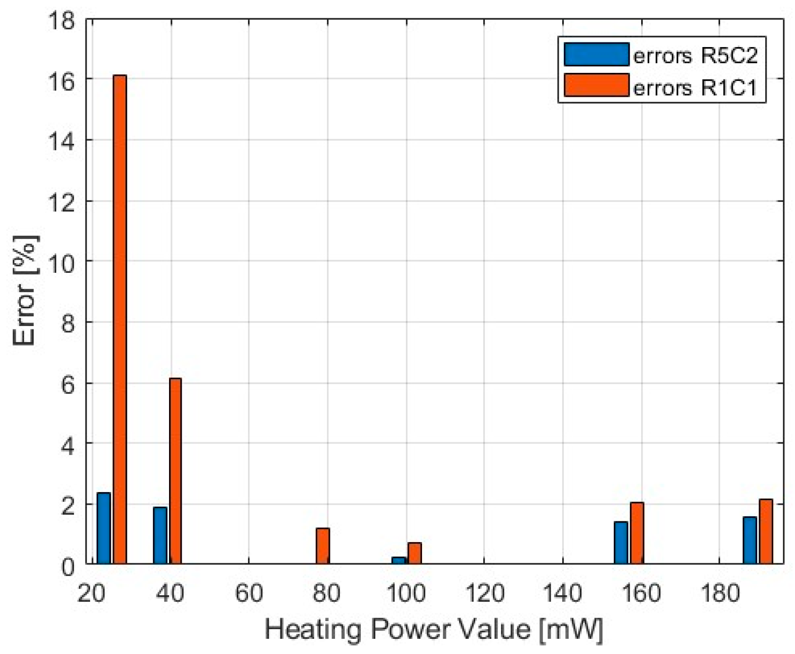
One can observe that both models’ responses remain approximately linear within the analyzed range. Compared to the commonly used R1C1 model, the C2R5 model applied to our non-adiabatic calorimeter resulted in an improvement across the entire range of calibrated power values. The most significant improvement in the estimated power accuracy is observed at low heating power levels, where the influence of heat from the transmitting coil represents a relatively large portion of the measured power. In this region, a noticeable increase in estimation accuracy is achieved, with the error decreasing from 16% for the R1C1 model to just 2.5% for the C2R5 model (Figure 7). Although the improvement in accuracy is less pronounced at higher power values, a reduction in error is still noticeable. For the upper calibration range, the error is reduced to approximately 1.5%.

4. Discussion

The results of our study demonstrate that our extended lumped-parameter thermal model can be effectively calibrated, offering a significant improvement over the corrected-slope method, which is widely used to measure the heating power of magnetic nanoparticles. This enhancement is particularly noticeable at low heating power values, where the influence of heat transfer from the excitation coil becomes a significant factor. By comparing our refined model to the traditional corrected-slope method, we observed a reduction in measurement errors, particularly at lower heating power values. The error analysis presented in Table 2 shows that for input power values around 25 mW, the relative error decreased from 16.09% to 2.36%, while for higher power values around 190 mW, the error reduction was more moderate, improving from 2.14% to 1.58%. This suggests that the refinements introduced in our model are particularly significant when the effects of external heat transfer cannot be neglected. Calibration using the global optimization toolbox provides a solution that minimizes error in the middle range of the calibrated values, while the error at the range boundaries remains relatively higher. In our model, identifying the source of heating power determination errors related to the heat flow generated by the excitation coil allowed us to eliminate large errors at low power values, thereby increasing measurement accuracy and leading to a more symmetric error distribution at both ends of the calibrated range.

Among the unmodeled sources affecting the remaining error, the most significant is the excessive heat transfer associated with factors such as the influence of ambient temperature on the sample. This is particularly relevant in the upper part of the calorimeter, where the sample is introduced into the system, and which is not covered by the water-cooling jacket. Addressing this issue would require considering the inhomogeneity of the calorimetric properties of the sample’s surroundings and potentially incorporating the thermal properties of the vessel walls containing the measured liquid.

Another source of error we must consider is the accuracy of the measurement probes, which is specified by the manufacturer’s calibration note at 0.1 °C. Additionally, errors arise from the process of setting and determining the input heating power, where the primary sources of uncertainty include the tolerance of the resistor and the precision and stability of the power supply voltage. However, rather than relying solely on the nominal tolerance of the resistor, we directly measured its resistance value using a precise Agilent 4263B LCR Meter (Santa Clara, CA, USA), which offers a basic accuracy of 0.1%. This approach allowed us to minimize uncertainty in power determination. It should be noted that the calculated error values refer to a system where heating power is generated by a concentrated heating element (SMD resistor) submerged in liquid. However, in the case of magnetic nanoparticle heating, energy dissipation is not specifically localized in space but rather more uniformly distributed throughout the sample volume. Previous studies [20,47] have repeatedly demonstrated that the temperature distribution within the sample is not perfectly homogeneous, mainly due to the uniformity of the magnetic field throughout the entire sample volume. This results in an additional source of error related to the positioning of the measurement probe. However, this type of error is not directly related to the calorimeter’s construction or a process affecting its non-adiabaticity and overall accuracy. Instead, it stems from calibration limitations caused by the lack of an available reference heating power source in the form of a nanoparticle solution.

Future work could explore the integration of the real-time monitoring of ambient temperature fluctuations or the adaptive control of the working cycles of the cooling system. Additionally, incorporating more complex models that capture spatial temperature variations within the sample and the calorimeter could provide even greater precision in calorimetric measurements. However, this would simultaneously increase the number of model parameters, complicate its structure, and require additional sensors for simultaneous measurements. Such modifications would also increase the computational complexity and extend the time required to find a solution through global optimization.

In this article, we present a model of a non-adiabatic calorimeter dedicated to measuring the SAR of superparamagnetic nanoparticles. However, it should be noted that the measurement uncertainty of SAR depends not only on effects related to the non-adiabatic nature of the measurement system in which the experiment is conducted but also on various other factors. According to some authors, the cumulative uncertainty can reach up to 14% [47]. This uncertainty is largely attributed to the heat loss generated by nanoparticles in the non-adiabatic calorimeter. Additionally, significant components of this error stem from the positioning of the fiber optic thermometer probe inside the sample, due to the inhomogeneity of the magnetic field inside the coil, particularly within the volume of the tested sample. This affects the non-uniform distribution of heating power within the sample.

Furthermore, the direct calculation of SAR using Formula (4) is as follows:

$$SAR={\displaystyle \frac{P}{m_{MNP}}}={\displaystyle \frac{P}{{\varphi }_{MNP}{V}_{MNP}}}$$

(4)

where $P$ is the heat power dissipated by the magnetic nanoparticles, $m_{MNP}$ is the mass of magnetic nanoparticles, and ${\varphi }_{MNP}$ and $V_{MNP}$ are the concentration and volume of the magnetic nanoparticle solution, respectively. Additional errors arise from inaccuracies in the reported concentration values or the measured sample volume. It is also important to consider that during long measurement durations, solvent evaporation may occur due to the insufficient sealing of the openings for the fiber optic probe or condensation on the walls of the sample container, introducing an additional source of error, which also affects the long-term calibration process.

Improving the measurement uncertainty of SAR is a multifactorial and complex task. The RC lumped-element model of a non-adiabatic calorimeter presented in this article maintains practical complexity while identifying the error sources associated with heat transfer from the transmitting coil. As a result, in the calibrated range of 20–200 mW, the measurement error related to the non-adiabatic nature of the calorimetric system was reduced to 2.5%.

5. Conclusions

In this study, we developed and validated an enhanced RC lumped-parameter calorimetric model for AC magnetometry, addressing the challenges of non-adiabatic heat transfer in heating power measurements of magnetic nanoparticles. Our approach improves upon the traditional corrected-slope method by incorporating the undesirable effects of heat flow from the excitation coil to the sample and its surroundings, as well as integrating the thermal parameters of the sample’s environment and employing multi-point temperature measurements.

The calibration protocol of the proposed non-adiabatic measurement system included 19 different heating power excitations, applied using a resistor-based heater with an adjustable resistive heating power and the heating power of the transmission coil. The influence of both these heating sources on the sample and its surroundings was integrated into the model. These measurement configurations were used to determine the model parameters via a global optimization algorithm from MATLAB’s global optimization toolbox. The results demonstrate that our refined model significantly reduces measurement errors, particularly at lower heating power values, where external heat transfer effects are most pronounced. Overall, our measurement system achieved an accuracy of less than 2.5% across the entire calibration range (20–200 mW) of heating powers, representing a substantial improvement over the corrected-slope method, which exhibited errors of up to 16% at low power levels.

The use of a direct current excitation coil during calibration allowed us to isolate and quantify the thermal effects of the coil’s heating without interference from eddy currents. This methodological innovation enabled simultaneous calibration measurements with different combinations of both excitation powers, effectively eliminating the additional heat source generated by eddy currents in the heater’s power delivery wires during the excitation of the transmission coil with alternating current.

Our findings provide a more accurate and reliable method for assessing the heating efficiency of magnetic nanoparticles compared to the corrected-slope method. The proposed lumped-parameter thermal model serves as a valuable tool for optimizing hyperthermia applications and advancing research in the field of magnetic nanoparticles.