
A Comparative Study of UCS Results Obtained from Triaxial Tests Under Multiple Failure State Conditions (Test Type II)


Abstract
1. Introduction

| # | Empirical Relationships | Method | Reference | Range of Input Parameters | UCS Range (MPa) | ||||
|---|---|---|---|---|---|---|---|---|---|
| ne (%) | Vp (m/s) | Rn (-) | |||||||
| L-Type | N-Type | From | To | ||||||
| 1 | UCS = 78.22ne + 201 | RA | [9] | 0.14–1.07 | – | – | – | 109.2 | 193.3 |
| 2 | UCS = 35.54Vp − 55 | RA | [9] | – | 4740–6690 | – | – | 109.2 | 193.3 |
| 3 | UCS = 8.36Rn(L) − 416 | RA | [9] | – | – | 64–72 | – | 109.2 | 193.3 |
| 4 | UCS = 2.208e0.067Rn(N) | RA | [10] | – | – | – | 23.9–73.4 | 11 | 259 |
| 5 | UCS = 1.4459e0.0706Rn(L) | RA | [11] | – | – | 20.00–65.76 | – | 6.32 | 196.5 |
| 6 | UCS = 0.9165e0.0669Rn(N) | RA | [11] | – | – | - | 23.00–75.97 | 6.32 | 196.5 |
| 7 | UCS = 4.24e0.059Rn(N) | RA | [12] | – | – | – | 48.30–61.80 | 60.8 | 202.9 |
| 8 | UCS = 124.28ne−0.56 | RA | [13] | 0.64–3.72 | – | – | – | 62.4 | 197 |
| 9 | UCS = 0.004Vp1.247 | RA | [13] | – | 2339–5753 | – | – | 62.4 | 197 |
| 10 | UCS = 0.0407Vp − 36.31 | RA | [14] | – | 1941–4751 | – | – | 23.77 | 161.7 |
| 11 | UCS = e(2.28lnRn(L)−4.04) | RA | [15] | – | – | 15–60 | – | 10.54 | 244.8 |
| 12 | UCS = 0.033Vp − 34.83 | RA | [16] | – | 1682–4657 | – | – | 32.51 | 133.5 |
| 13 | UCS = 2.38e0.065Rn(L) | RA | [17] | – | – | 25.89–67.07 | – | 17.55 | 198.2 |
| 14 | UCS = 0.087Vp − 355.8 | RA | [17] | – | 5384–6250 | – | – | 91.48 | 198.2 |
| 15 | UCS = 228.2e(−1.98ne) | RA | [17] | 0.06–0.4 | – | – | – | 91.48 | 198.2 |
| 16 | UCS = −17.88ln(ne) + 60.22 | BHM | [18] | 0.52–7.23 | – | – | – | 20.3 | 112.9 |
| 17 | UCS = 8.17e0.0004Vp + 3.93 | BHM | [18] | – | 1160–5935 | – | – | 20.3 | 112.9 |
| 18 | UCS = 7.03e0.0386Rn(L) + 8.39 | BHM | [18] | – | – | 16.8–55.7 | – | 20.3 | 112.9 |
| 19 | UCS = 4.15e0.0386Rn(L) + 6.08e0.0004Vp − 8.22 | BHM | [18] | – | 1160–5935 | 16.8–55.7 | - | 20.3 | 112.9 |
| 20 | UCS = 6.32e0.0004Vp − 9.6ln(ne) + 20.5 | BHM | [18] | 0.52–7.23 | 1160–5935 | – | – | 20.3 | 112.9 |
| 21 | UCS = 3.26e0.0386Rn(L) + 5.84e0.0004Vp − 3.56ln(ne) + 0.53 | BHM | [18] | 0.52–7.23 | 1160–5935 | 16.8–55.7 | – | 20.3 | 112.9 |
| 22 | UCS = 1.910Rn(N) − 10.3 | RA | [19] | – | – | – | 10–72 | 8 | 149 |
| 23 | UCS = 25.952e0.030Rn(L) | RA | [20] | – | – | 18–61 | – | 39 | 211.9 |
| 24 | UCS = 0.005Vp1.141 | RA | [20] | – | 2823–7943 | – | – | 39 | 211.9 |
| 25 | UCS = 0.004Rn(L)2.5972 | RA | [21] | – | – | 18.8–60 | – | 6.12 | 148 |
| 26 | UCS = 181.58ln(Vp) − 1443.9 | RA | [22] | – | 4108–7943 | – | – | 50.2 | 211.9 |
| 27 | UCS = 6.311Rn(L) − 194.92 | RA | [22] | – | – | 40–61 | – | 50.2 | 211.9 |
| 28 | UCS = 0.0367Vp − 31.18 | [23] | |||||||
| Equations (Reference) | Ref. | Correlation Coefficient (r) | Units and Notations | Rock Type | Number of Data |
|---|---|---|---|---|---|
| UCS = ax + b | [24] | 0.85 | -- | Sandstones | -- |
| UCS = 0.0642 Vp − 117.99, (MPa) | [25] | 0.90 | Vp: m/s | Sandstone, coal, quartz mica schist, phyllite, basalt | 43 |
| UCS = 56.71 Vp − 192.93, (MPa) | [26] | very small | -- | Cement mortar, sandstone, limestone | 75 |
| UCS = aVpb | [27] | 0.94 | -- | A wide range of British rock types | 150 |
| UCS = 9.95 Vp1.21, (MPa) | [28] | 0.83 | Vp: km/s | Marl, limestone, dolomite, sandstone, haematite, serpantine, diabase, tuff | 48 |
| Vp = 0.00317 UCS + 2.0195 | [29] | 0.80 | -- | -- | |
| UCS = 0.78 e0.88Vp | [30] | 0.73 | Vp: km/s | Volcanic group | -- |
| UCS = 0.78 Vp0.88 | [30] | 0.73 | Vp: km/s | Volcanic group | -- |
| UCS = 0.0407 Vp − 36.31, (N/mm2) | [14] | 0.85 | -- | 19 | |
| UCS = k ρ Vp2 + A, (kg/cm2) | [31] | ρ: g/cm3, Vp: km/s | -- | -- | |
| UCS = 0.036 Vp − 31.18, (MPa) | [23] | Vp: m/s | -- | -- | |
| UCS = 0.1564 Vp − 692.41, (MPa) | [32] | 0.90 | Vp: m/s | Sandstones | 9 |
| UCS = 0.0144 Vp − 24.856, (MPa) | [32] | 0.71 | Vp: m/s | Sandstones | 24 |
| UCS = 7.1912 Vp + 26.258, (MPa) | [33] | 0.57 | Vp: km/s | Sandstone, gravel stone, limestone, mudstone, shale | 8 |
| UCS = 21.677 Vp + 21.427 | [34] | 0.95 | Vp: km/s | Limestone, marble, dolomitic limestone, tuff, basalt | 8 |
| UCS = 0.0188 Vp + 0.0648 | [35] | 0.95 | Vp: km/s | Sandstone | -- |
| UCS = 2.304 Vp2.4315 | [36] | 0.97 | Vp: km/s | Diorite, quartzite, sandstone, limestone, marble, granadiorite, basalt, travertine, trachyte, tuff, andesite | 19 |
| UCS = 12.746 Vp1.194 | [4] | 0.79 | Vp: km/s | Limestone, sandstone, travertine, marl, dolomite, mudrock-shale, slate, siltstone | 97 |
| UCS = −7.155 + 6.194 Vp + 9.774 TS | [4] | 0.88 | Vp: km/s | 43 | |
| UCS = −10.029 + 5.734 Vp + 10.876 TS − 2.408 Is | [4] | 0.90 | Vp: km/s | 26 | |
| UCS = 9.95Vp1.21 | [37] | Diabase, dolomite, haematite, limestone, marl, sandstone, serpentine, tuff | |||
| UCS = 0.0028Rn(L)2.584 | [38] | Limestone, schist, travertine | |||
| UCS = (Vp − 2.0195)/0.0317 | [39] | Limestone, Marble, Dolomitic limestone, Dolomite, Gravelled limestone |
2. Brief Introduction to Triaxial Tests
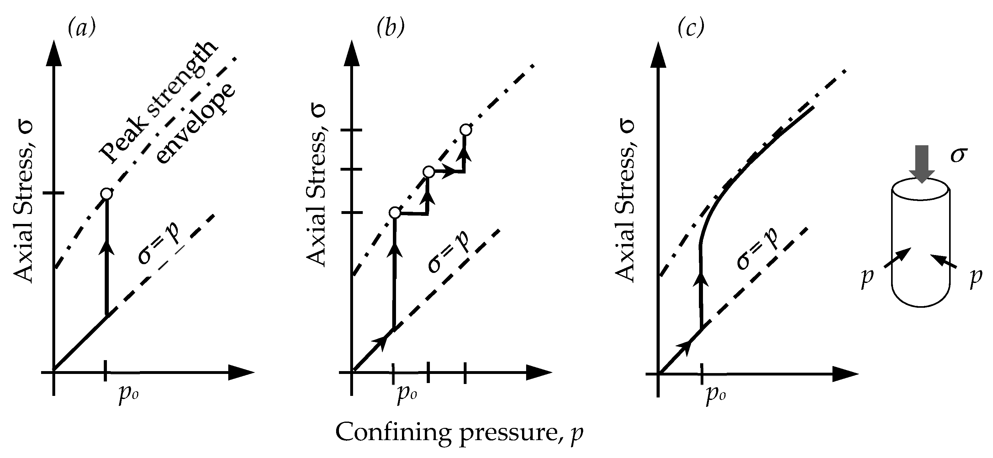
- Type I: An individual rock specimen is tested with a single pre-set confinement. It is required to perform at least three tests with three different confinements in order to obtain the peak strength envelope. This means that at least three samples are required to fulfil the test and construct the peak strength envelope. Typical results of one test are presented in Figure 1a and Figure 2a;
- Type II: Three different confinement levels are applied in the same sample. At each confinement level, the sample is tested until it tangents its peak strength at that confinement level, and then the confinement is changed to the next level for the test to continue. With the three different confinement levels in one test, it is possible to construct the peak strength envelope for the sample from only one test. Typical results of one test are presented in Figure 1b and Figure 2b;
- Type III: The test is carried out with the initial confinement until the sample tangents its peak strength. The linear portion of the axial stress versus axial strain curve has a slope of V (V = E is the Young’s modulus of the sample). After the initial step, the confinement and the axial stress are simultaneously increased in such a way that the obtained axial stress versus axial strain curve has the same slope as V. Typical results of one test are presented in Figure 1c and Figure 2c.
- Fitting a curve based on the results from triaxial tests. Depending on the behaviour of the rock, the fitting curve can be linear or non-linear;
- Plotting the strength envelope in a graph where the vertical axis represents the major principal stress (normally the axial stress during the triaxial test) and the horizontal axis represents minor principal stress (normally the confinement during the triaxial test);
- Extending the strength envelope until it intersects the vertical axis (at this point, the minor principal stress is zero). This intersection point can be interpreted as the UCS of the sample.
3. The Performed Test Procedure and Apparatus
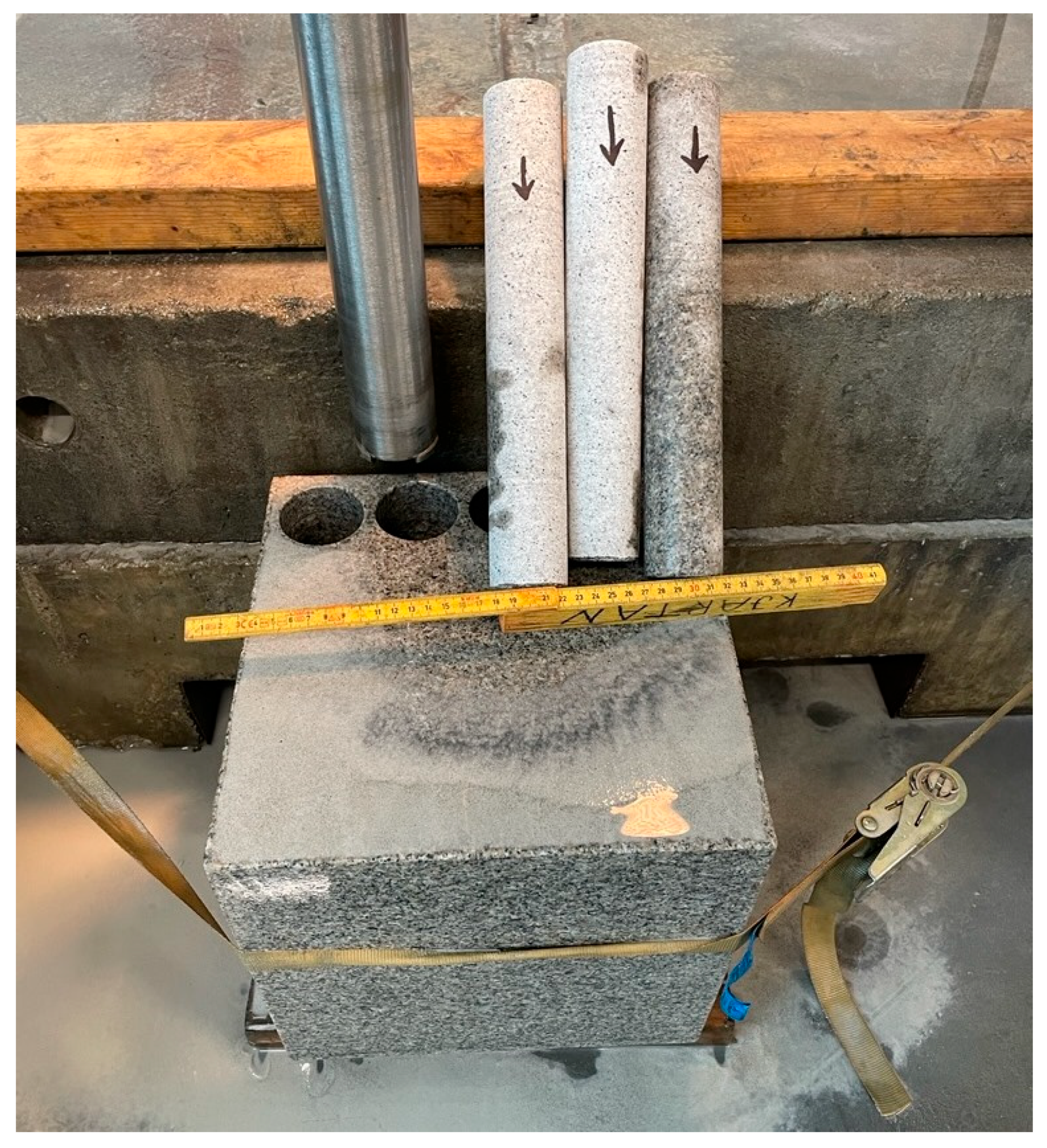
3.1. Sample Preparation
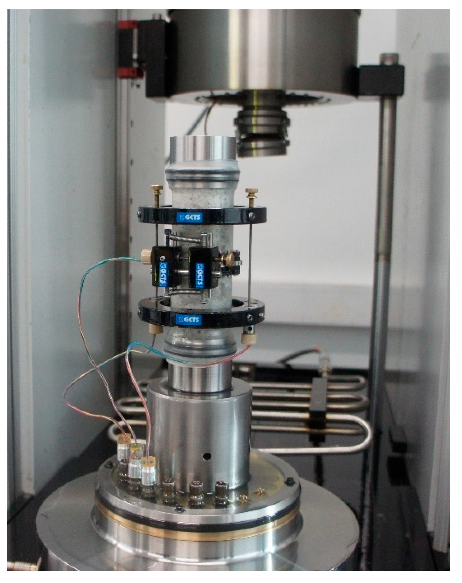
3.2. Test Apparatus
3.3. The Various Steps of the Test
- In “Step-0 MPa” in this test, the indication of corresponding peak strength is accurately monitored with no or minimum disturbance to the sample. This is achieved by high-frequency readings with clear and continuous plotting of the stress–strain curve, strict control of the speed of loading (based on the axial or radial strain rate), and an experienced operator;
- In principle, three loading steps after “Step-0 MPa” are sufficient but in our tests, five loading steps were used with selected confinement levels. The purpose of the five loading steps and the selected confinement levels is (a) to have more points for constructing the peak strength envelope, and (b) to observe the rock behaviour in a wide range of confinement.
4. Test Results
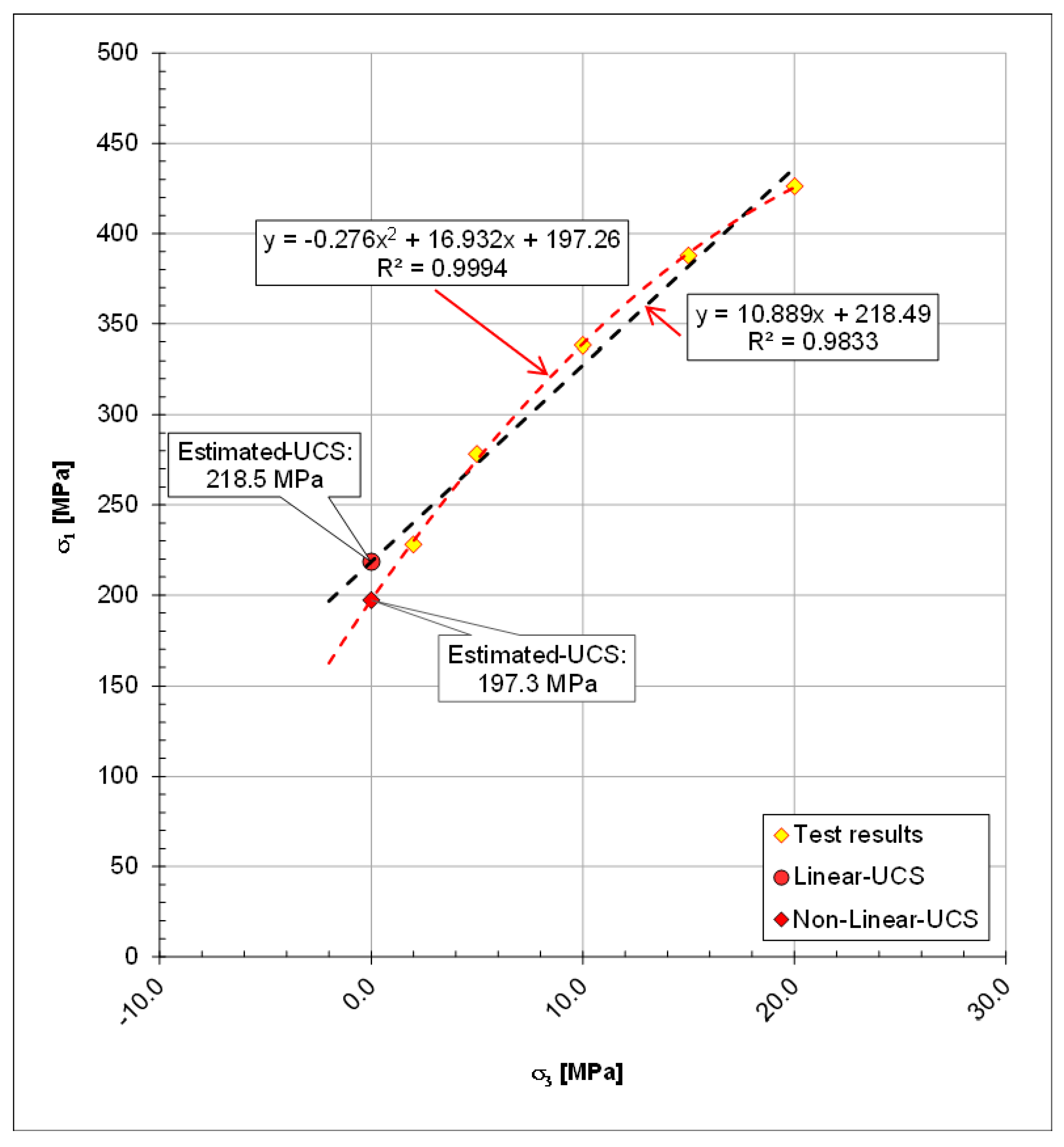
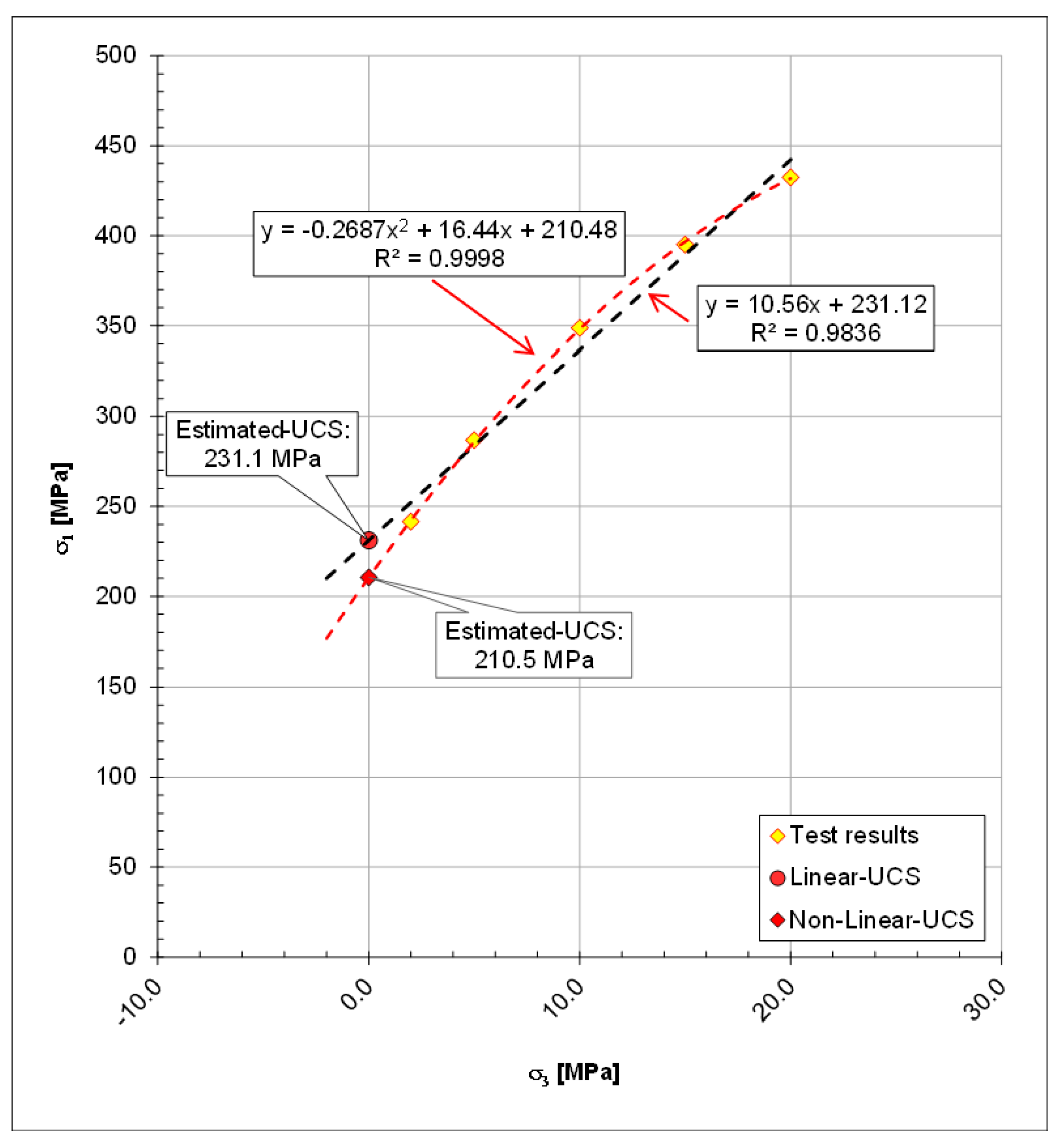
5. Estimating UCS Using Linear and Parabolic Equations
- Equation (1) is actually the Mohr–Coulomb failure criterion written in the form of principal stresses;
- σ1 and σ3 are major and minor principal stresses, respectively;
- k, σci,a, b, and c are the fitting parameters. The fitting parameters are defined by using the test results and a fitting procedure;
- k is related to the internal friction angle (ϕ) of the rock with the equation as k = (1 + sin(ϕ))/(1 − sin(ϕ));
- σci is also the UCS of the intact rock.
- The “Estimated-UCS” using parabolic fitting for sample A provided almost identical results with the “True-UCS” (197.26 versus 197.74 MPa, respectively, means a −0.2% error);
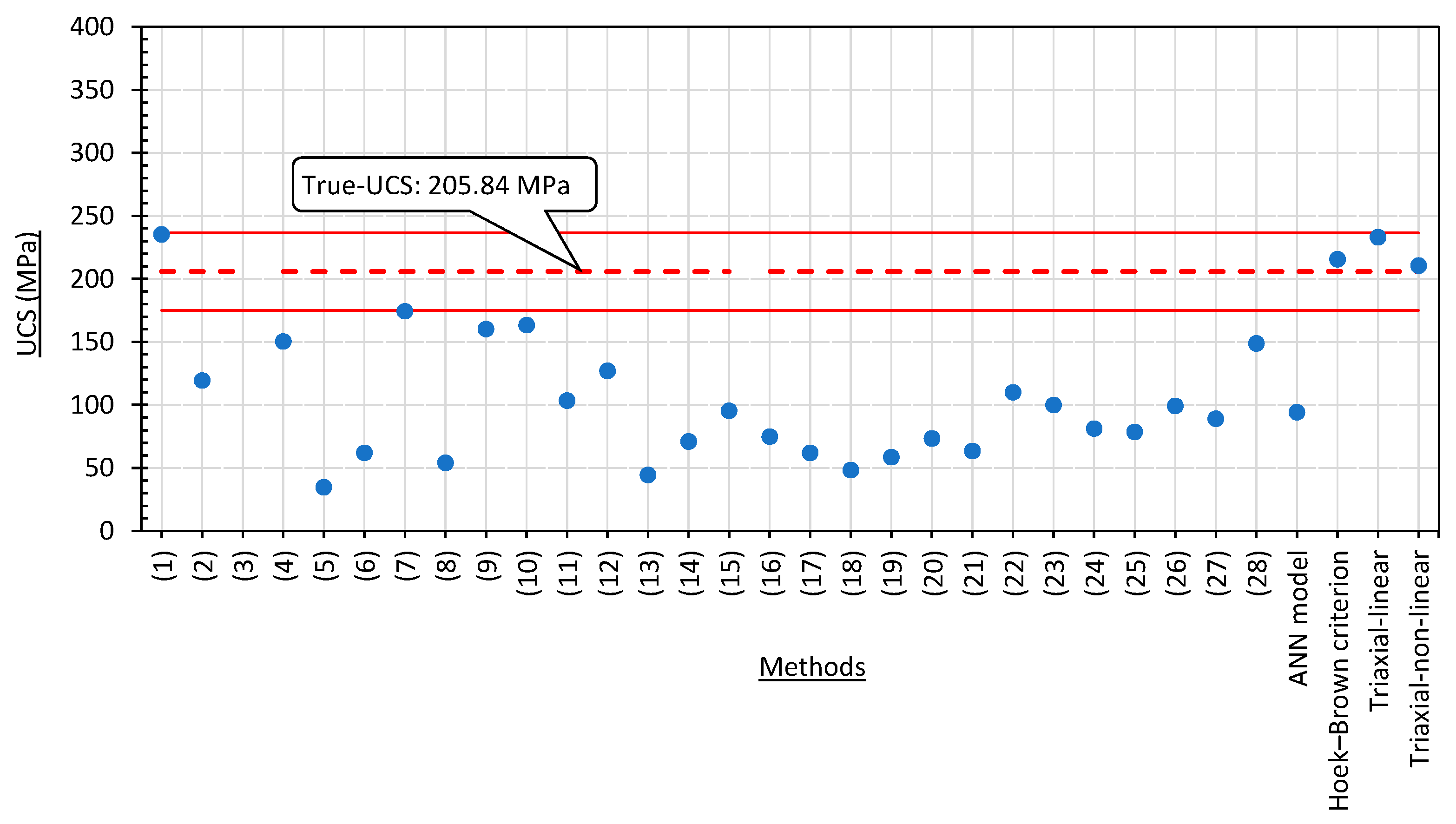
- For sample B, the “True-UCS” is 205.84 MPa, whilst the “Estimated-UCS” using the parabolic equation is 210.48 MPa (means a 2.2% error);
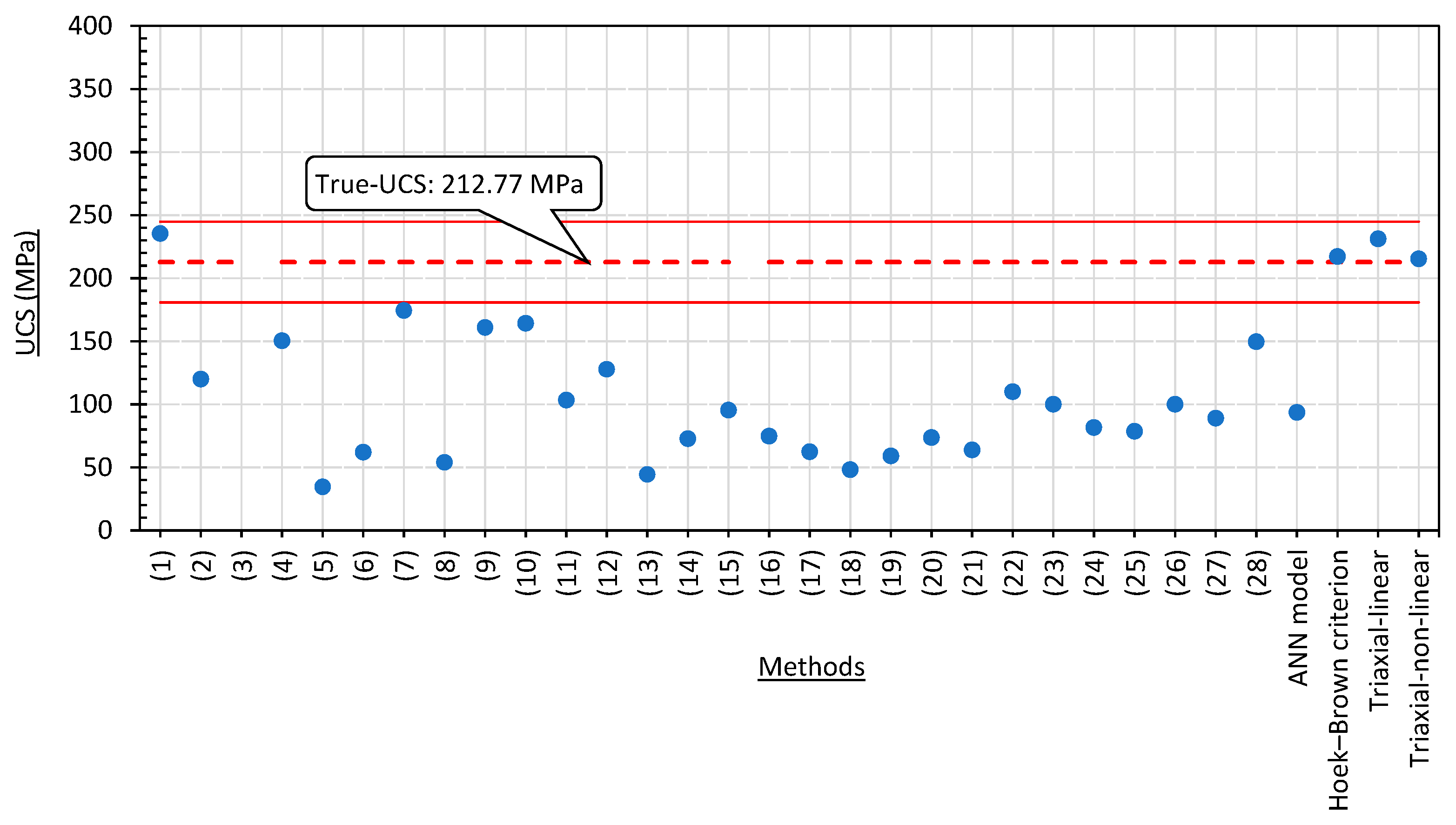
- For sample C, the “True-UCS” is 212.77 MPa, whilst the “Estimated-UCS” using the parabolic equation is 215.47 MPa (means a 1.3% error).
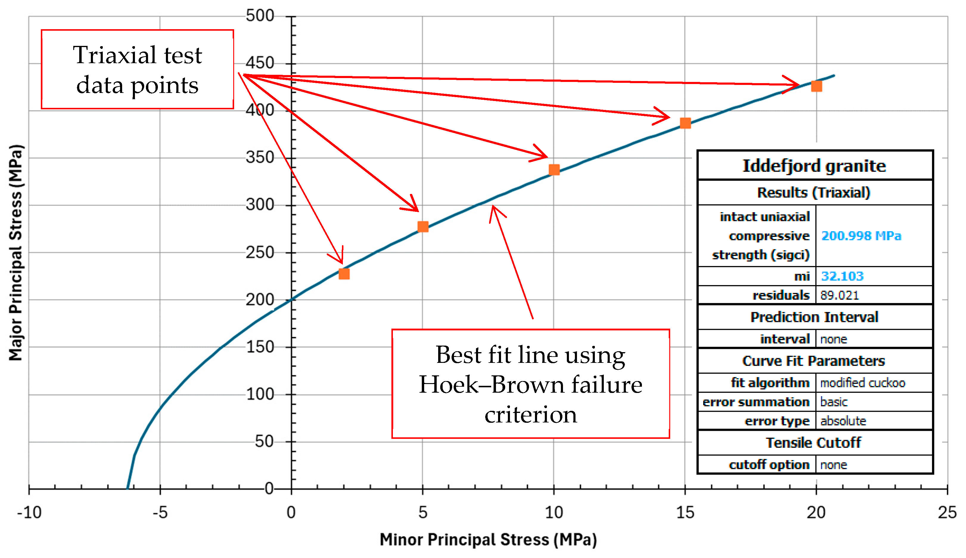
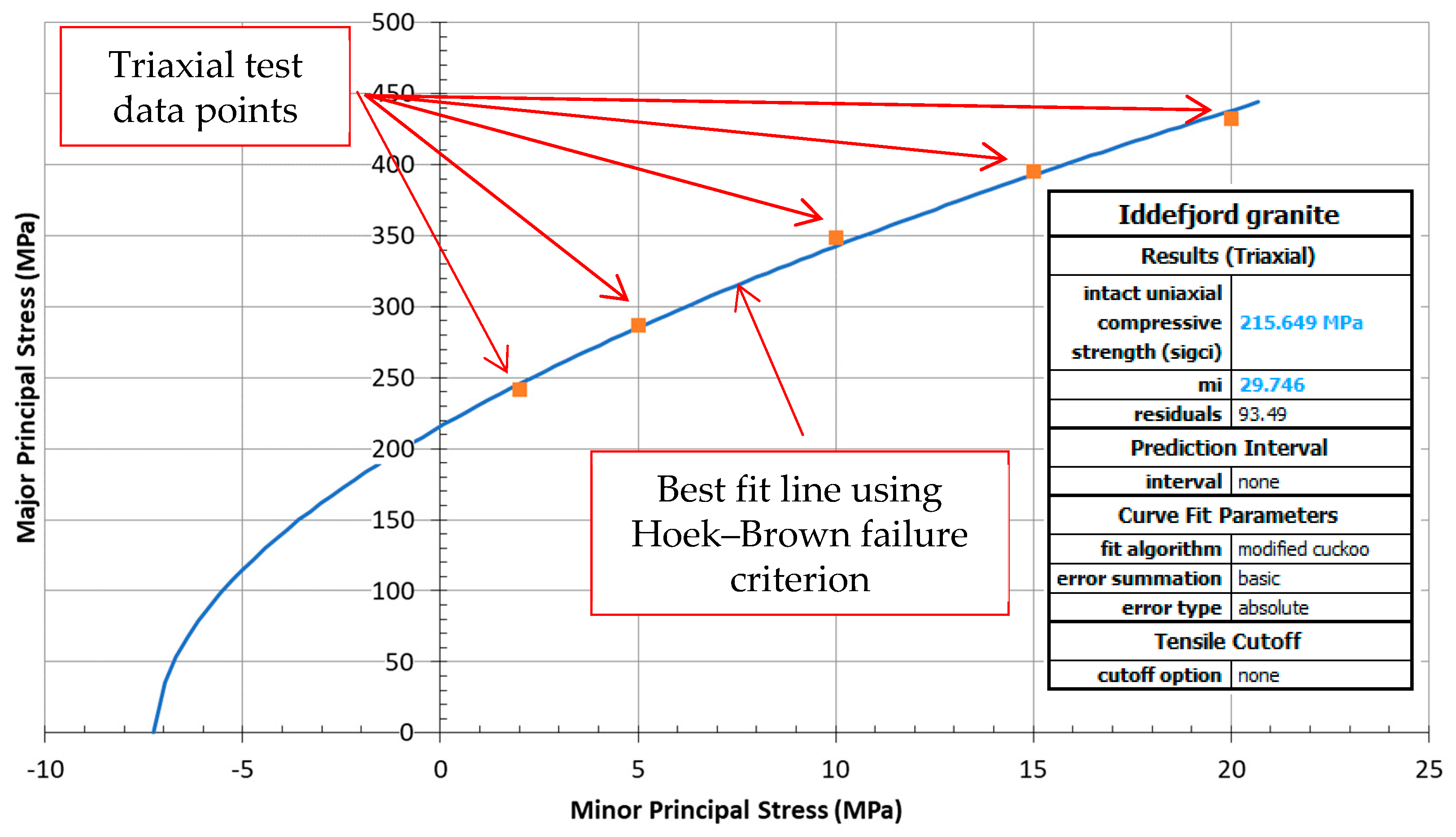
6. Estimating UCS Using Hoek–Brown Criterion Equation
- σ1 and σ3 are major and minor principal stresses, respectively;
- σci is the uniaxial compressive strength of the intact rock;
- mi is a material constant for the intact rock.
7. Comments on the Fitting Work
- In the linear fitting equation, the slope of the equation (parameter k) for samples A, B, and C is 10.89, 10.56, and 10.34, respectively. With these values of k, the corresponding internal friction angle for the rock samples are 56, 56, and 55 degrees, respectively.
- The values of “Estimated-UCS” obtained by the linear fitting equation (parameter σci), by parabolic fitting equation (parameter c), and by the Hoek and Brown criterion equation (parameter σci) are not too far from each other, as presented in Table 7;
- The obtained parameter mi for samples A, B, and C are 32, 30, and 29, respectively. These values are very much comparable to the recommended mi-value in such programs as RocLab and RocData [44], which is 32 ± 3 for granite;
- The obtained fitting parameters (k, a, b, and c) are relatively close for all samples A, B, and C. This is because the granite in this study is relatively homogenous. It is important to note that the fitting parameters are sample-dependent. Due to the inhomogeneous nature of rock, different rock types or even different samples from the same rock type have different UCS values. Consequently, they should have their own fitting parameters for each individual sample. Thus, it is not recommended to use the obtained fitting parameters in this study as general parameters for other cases. Instead, the form of equations can be used but the fitting parameters for each sample will be estimated directly from the obtained data of triaxial testing for that particular sample;
- The linear and parabolic fitting equations were obtained by built-in function in Excel. The Hoek–Brown fitting equation was obtained from commercial code RocData as mentioned or the “Goal Seek” in Excel can also be used. The mathematical algorithm behind both situations is the least squares method. Interested readers are recommended to refer to different mathematical books for more information on the method;
- The error between “Estimated-UCS” and “True-UCS” comes from two sources, which are (a) the sample’s behaviour and (b) the selection of the fitting equation. If the sample expresses uniform behaviour at every loading step, then it is easier to find a good fitting equation for the tests and vice versa. The right choice of fitting equation will also contribute significant error to the estimate. As demonstrated above, the linear fitting equation gives a larger error than the non-linear equation for the Iddefjord granite samples performed in this research.
8. Comparison of the Estimated UCS with Other Empirical Methods
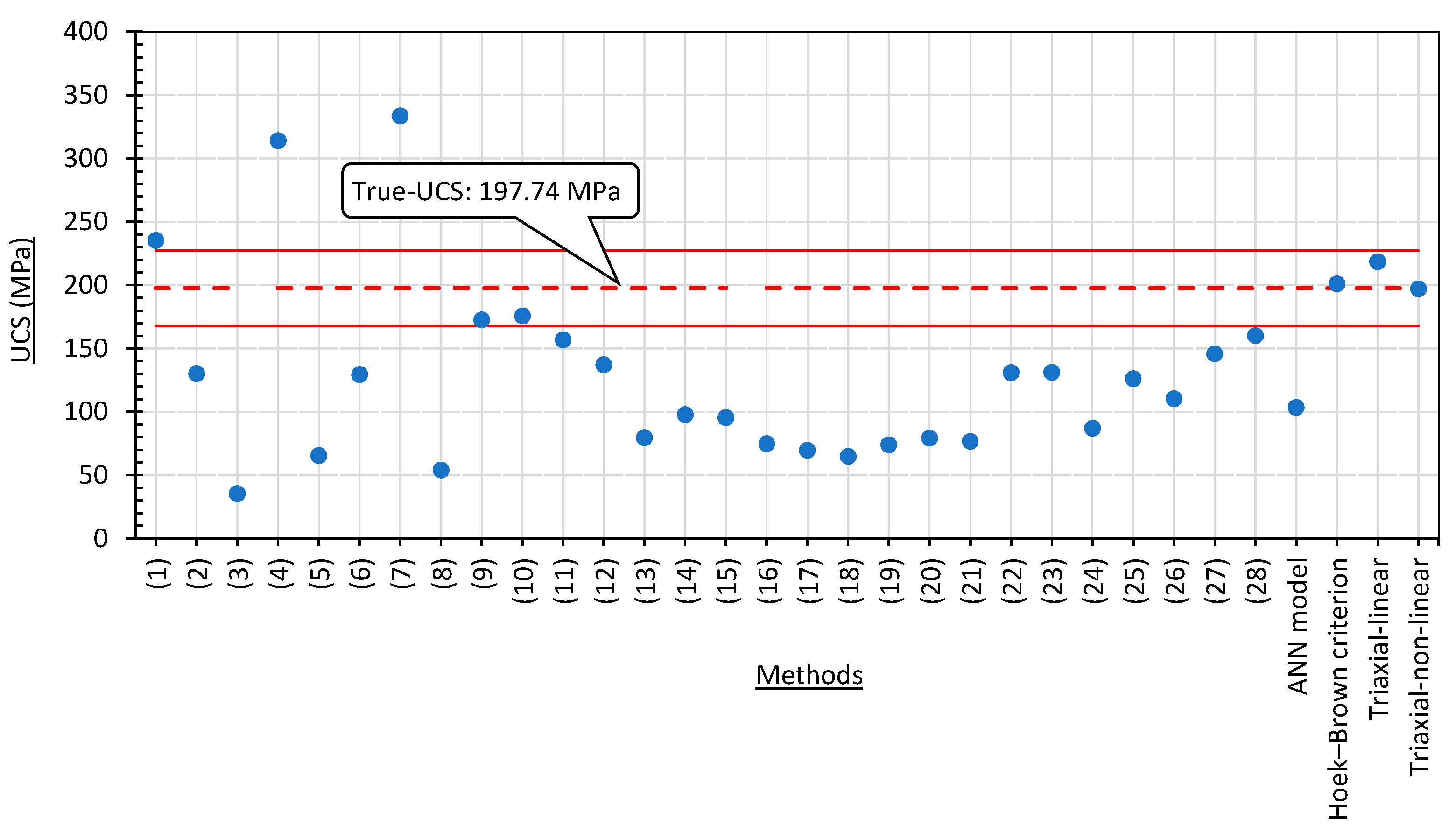
- There is a large variety in the results from empirical methods. Most of the empirical methods underestimate the UCS. Results from most of the methods were less than 75% of the “True-UCS”, and some methods even provided a negative value—meaning tension. These poor results are considered as not acceptable. The reason for such poor results may be that each empirical method may have certain limitations of the database and applicable range;
- It seems that method (1) proposed by Tuğrul and Zarif [9] is able to give reasonable estimates for all three samples;
- Some other correlations in Table 2 were randomly tested and it is interesting to find that the equation proposed by Sharma and Singh [25] gives good estimates for all three samples (within ±15% of deviation), even though the study by Sharma and Singh did not cover granitic rock. Unfortunately, there are only three samples in our study so we are not able to comment more on this method other than that our granite samples also support Sharma and Singh’s proposed equation;
- It is not clear in the empirical and ANN methods if their estimated UCS is corresponding to a 50 mm core or other core diameters. It is assumed in this paper that the empirical and ANN methods estimate UCS with a 50-millimeter core diameter;
- The results from method (1) are relatively good for all three samples. The level of error between the results from this method and the “True-UCS” is approximately 15%, which is an accuracy considered acceptable for empirical methods;
- The error between the “Estimated-UCS” based on triaxial tests and the “True-UCS” is within 15% for all tests in this study. With the linear fitting equation, the error is from 9.5 to 13.4%; with the parabolic fitting equation, the error is from −0.2 to 2.3%; and with the Hoek–Brown criterion equation, the error is from 1.7 to 4.8%. The non-linear fitting equations provided much more accurate results than the linear fitting equation in this particular test dataset.
9. Discussion of the Test and Obtained Results
- Estimating UCS with empirical methods resulted in a very large variation. Based on 32 empirical methods, calculations yielded results ranging from “−40” to “+330” MPa (“–” means tension, and “+” means compression) for the three granite samples in this research with an expected UCS of about 200 MPa. One probable cause could be that each empirical method is suitable within the limitations of the database that was used to build such empirical formulae. It seems that method (1) produced reasonable estimates compared to the “True-UCS” for all three samples in this research. The rest of the methods, including the ANN model, failed to give results for all three samples that fit to the “True-UCS”;
- On the other hand, the “Estimated-UCS” values based on the triaxial test were close to the “True-UCS” for all three samples in this research. The error between the “Estimated-UCS” based on triaxial tests and the “True-UCS” is within 15% (when using linear fitting equations) and within 5% (when using non-linear fitting equations). It is obvious that non-linear fitting equations provided results with much smaller error than the linear fitting for the test in this research. This may be due to the persistent behaviour of the Iddefjord granite;
- The reliability of the “Estimated-UCS” based on the results from the triaxial test can be evaluated by studying the behaviour of the tested rock sample and the obtained rock strengths at different confinements. Normally, a better coefficient of determination (R2—closer to 1) indicates a more reliable “Estimated-UCS”;
- The triaxial test performed in this research is triaxial test Type II. The method can also be applied for triaxial test Type III as the strength envelope is built for each individual rock sample. The use of results from triaxial test Type I may reduce the accuracy of the “Estimated-UCS” as test Type I is performed on different rock samples, and the inhomogeneity between the samples will have a negative impact on the accuracy of the calculation process;
- It is noted that the triaxial test and the UCS test might be different in the end effects, frictional constraints, alignment of the sample, failure mechanisms, loading rate, and loading path. However, if the triaxial test and UCS test follow a certain standard or method (ISRM’s suggested method for example), then the “Estimated-UCS” is expected to be comparable to the result from a conventional UCS test. As stated in this study, the NTNU/SINTEF laboratory has a comprehensive UCS database (which was obtained by using conventional UCS tests) for Iddefjord granite. The “Estimated-UCS” values obtained from the triaxial test data were compared to the database and found reasonable;
- It is necessary to mention again that the triaxial test procedure in this research study was not conventional. The first stage of the triaxial tests in this research (with zero confinement) was performed to facilitate the comparison between the “True-UCS” and “Estimated-UCS” on the same sample in order to demonstrate the reliability of the method. In a normal triaxial test Type II, the test will always start with a certain confinement. The zero-confinement step in our test procedure may cause some disturbance to the rock samples before carrying out the subsequent non-zero-confinement steps. This is similar to the limitation of the triaxial test Type II itself—after every testing step, the sample responds with a certain disturbance. To keep this disturbance at a minimum level, it requires an experienced operator to stop and move forward the test at the right moment—not too early (causing underestimation of peak strength) and not too late (causing too much disturbance to the sample leading to underestimation of the rock strength).
10. Conclusions and Concluding Remarks
- UCS estimated with empirical methods resulted in a very large variation. Only two out of twenty-nine empirical methods were able to provide the “Estimated-UCS” close to the “True-UCS” (within 15% of error). Thus, great care should be given when using empirical formulae for estimating the UCS;
- The “Estimated-UCS” based on results from the triaxial test is close to the “True-UCS” for all three samples in this research. The behaviour of the rock sample can be observed directly from the test results. Based on the observed behaviour, a proper fitting function (linear or non-linear) can be selected. The reliability of the calculation can also be evaluated based on the value of the coefficient of determination (R2) of the fitting equations;
- It can be stated that it is a much more reliable way to estimate UCS based on results from the triaxial test Type II than using empirical formulae, as demonstrated herein. With a proper fitting equation used, the error of this method can be less than 2.5%. With such accuracy, UCS can be considered to be an additional relevant outcome of triaxial test Type II;
- The method described herein is not limited to granite as used in this research, rather, it is expected to be a universal tool for all hard rock samples. The limitations in using this method for other rock types are just the same as for performing an ordinary triaxial test Type II. For example, too-brittle rock types are not suitable for triaxial tests as the sample will be broken and completely destroyed at a very early stage of the triaxial test Type II. Otherwise, the estimation of UCS can be calculated as soon as a triaxial test Type II has been performed successfully;
- The approach of determining UCS based on triaxial testing has been demonstrated after successfully applying a triaxial test Type II. This method can be applied for triaxial test Type III. The method might be applied with triaxial test Type I, however, inhomogeneity between rock samples will have a greater impact on the accuracy of the calculation when using results from this test type.
Author Contributions
Funding
Institutional Review Board Statement
Informed Consent Statement
Data Availability Statement
Acknowledgments
Conflicts of Interest
Abbreviations
| ANN | Artificial neural network |
| ASTM | American Society for Testing and Materials |
| BHM | Bayesian hierarchical modelling |
| BTS | Brazilian tensile strength |
| Is50 | Point load index |
| ISRM | International Society for Rock Mechanics and Rock Engineering |
| γd | Dry density |
| ne | Effective porosity |
| nt | Total porosity |
| RA | Regression analysis |
| Rn | Schmidt hammer rebound number |
| Rn(N) | Schmidt hammer rebound number for N-type |
| Rn(L) | Schmidt hammer rebound number for L-type |
| SDI | Slake durability index |
| UCS | Uniaxial compressive strength |
| Vp | Pulse velocity |
| Vs | Shear wave velocity |
References
- ISRM. Suggested Methods for Determining the Uniaxial Compressive Strength and Deformability of Rock Materials; International Society for Rock Mechanics: Lisbon, Portugal, 1979; 4p, Available online: https://isrm.net/isrm/page/show/1305 (accessed on 9 March 2025).
- ISRM. Suggested Methods for Determining the Strength of Rock Materials in Triaxial Compression: Revised Version; International Society for Rock Mechanics: Lisbon, Portugal, 1983; 6p. [Google Scholar]
- ASTM D7012-13; Standard Test Methods for Compressive Strength and Elastic Moduli of Intact Rock Core Specimens under Varying States of Stress and Temperatures. American Society of Testing and Materials: West Conshohocken, PA, USA, 2014. Available online: https://www.astm.org/d7012-13.html (accessed on 9 March 2025).
- Altindag, R. Correlation between P-wave velocity and some mechanical properties for sedimentary rocks. J. S. Afr. Inst. Min. Metall. 2012, 112, 229–237. [Google Scholar]
- Le, T.-T.; Skentou, A.D.; Mamou, A.; Asteris, P.G. Correlating the Unconfined Compressive Strength of Rock with the Compressional Wave Velocity Effective Porosity and Schmidt Hammer Rebound Number Using Artificial Neural Networks. Rock Mech. Rock Eng. 2022, 55, 6805–6840. [Google Scholar] [CrossRef]
- Skentou, A.D.; Bardhan, A.; Mamou, A.; Lemonis, M.E.; Kumar, G.; Samui, P.; Armaghani, D.J.; Asteris, P.G. Closed-Form Equation for Estimating Unconfined Compressive Strength of Granite from Three Non-destructive Tests Using Soft Computing Models. Rock Mech. Rock Eng. 2022, 56, 487–514. [Google Scholar] [CrossRef]
- Wang, M.; Wan, W. A new empirical formula for evaluating uniaxial compressive strength using the Schmidt hammer test. Int. J. Rock Mech. Min. Sci. Géoméch. Abstr. 2019, 123, 104094. [Google Scholar] [CrossRef]
- Wang, M.; Wan, W.; Zhao, Y. Prediction of the uniaxial compressive strength of rocks from simple index tests using a random forest predictive model. C. R. Mec. 2020, 348, 3–32. [Google Scholar] [CrossRef]
- Tuğrul, A.; Zarif, I.H. Correlation of mineralogical and textural characteristics with engineering properties of selected granitic rocks from Turkey. Eng. Geol. 1999, 51, 303–317. [Google Scholar] [CrossRef]
- Katz, O.; Reches, Z.; Roegiers, J.C. Evaluation of mechanical rock properties using a Schmidt Hammer. Int. J. Rock Mech. Min. Sci. 2000, 37, 723–728. [Google Scholar] [CrossRef]
- Aydin, A.; Basu, A. The Schmidt hammer in rock material characterization. Eng. Geol. 2005, 81, 1–14. [Google Scholar] [CrossRef]
- Fener, M.; Kahraman, S.; Bilgil, A.; Gunaydin, O. A comparative evaluation of indirect methods to estimate the compressive strength of rocks. Rock Mech. Rock Eng. 2005, 38, 329–343. [Google Scholar] [CrossRef]
- Sousa, L.M.; del Río, L.M.S.; Calleja, L.; de Argandona, V.G.R.; Rey, A.R. Influence of microfractures and porosity on the physico- mechanical properties and weathering of ornamental granites. Eng. Geol. 2005, 77, 153–168. [Google Scholar] [CrossRef]
- Vasconcelos, G.; Lourenço, P.B.; Alves, C.A.S.; Pamplona, J. Ultra-sonic evaluation of the physical and mechanical properties of granites. Ultrasonics 2008, 48, 453–466. [Google Scholar] [CrossRef]
- Bruno, G.; Vessia, G.; Bobbo, L. Statistical method for assessing the uniaxial compressive strength of carbonate rock by Schmidt hammer tests performed on core samples. Rock Mech. Rock Eng. 2013, 46, 199–206. [Google Scholar] [CrossRef]
- Khandelwal, M. Correlating P-wave velocity with the physico-mechanical properties of different rocks. Pure Appl. Geophys. 2013, 170, 507–514. [Google Scholar] [CrossRef]
- Mishra, D.A.; Basu, A. Estimation of uniaxial compressive strength of rock materials by index tests using regression analysis and fuzzy inference system. Eng. Geol. 2013, 160, 54–68. [Google Scholar] [CrossRef]
- Ng, I.T.; Yuen, K.V.; Lau, C.H. Predictive model for uniaxial com- pressive strength for Grade III granitic rocks from Macao. Eng. Geol. 2015, 199, 28–37. [Google Scholar] [CrossRef]
- Tandon, R.S.; Gupta, V. Estimation of strength characteristics of different Himalayan rocks from Schmidt hammer rebound, point load index, and compressional wave velocity. Bull. Eng. Geol. Environ. 2015, 74, 521–533. [Google Scholar] [CrossRef]
- Armaghani, D.J.; Tonnizam Mohamad, E.; Momeni, E.; Monjezi, M.; Sundaram Narayanasamy, M. Prediction of the strength and elasticity modulus of granite through an expert artificial neural network. Arab. J. Geosci. 2016, 9, 48. [Google Scholar] [CrossRef]
- Çelik, S.B.; Çobanoğlu, I. Comparative investigation of Shore, Schmidt, and Leeb hardness tests in the characterization of rock materials. Environ. Earth Sci. 2019, 78, 554. [Google Scholar] [CrossRef]
- Li, D.; Armaghani, D.J.; Zhou, J.; Lai, S.H.; Hasanipanah, M. A GMDH predictive model to predict rock material strength using three non-destructive tests. J. Nondestruct. Eval. 2020, 39, 1–14. [Google Scholar] [CrossRef]
- Goktan, R.M. Theoretical and Practical Analysis of Rock Rippability. Ph.D. Thesis, Istanbul Technical University, Istanbul, Turkey, 1988. [Google Scholar]
- Cheng, H.; Hu, Z.Y. Some factors affecting the uniaxial strength of weak sandstone. Bull. Eng. Geol. Environ. 2003, 62, 323–332. [Google Scholar] [CrossRef]
- Sharma, P.K.; Singh, T.N. A correlation between P-wave velocity, impact strength index, slake durability index and uniaxial compressive strength. Bull. Eng. Geol. Environ. 2007, 67, 17–22. [Google Scholar] [CrossRef]
- Çobanoğlu, İ.; Çelik, S.B. Estimation of uniaxial compressive strength from point load strength, Schmidt hardness and P-wave velocity. Bull. Eng. Geol. Environ. 2008, 67, 491–498. [Google Scholar] [CrossRef]
- McCann, D.M.; Culshaw, M.G.; Northmore, K.J. Rock mass assessment from seismic measurements. Geol. Soc. Lond. Eng. Geol. Spec. Publ. 1990, 6, 257–266. [Google Scholar] [CrossRef]
- Christaras, B.; Mariolakos, I.; Foundoulis, J.; Athanasias, S.; Dimitriou, A. Geotechnical input for the protection of some Macedonian Tombs in Northern Greece. In Proceedings of the 6th International Symposium Conservation of Monuments in the Mediterranean Basin, Rhodes, Greece, 6–11 May 1997; pp. 125–132. [Google Scholar]
- Yasar, E.; Erdogan, Y. Correlating sound velocity with the density, compressive strength and Young’s modulus of carbonate rocks. Int. J. Rock Mech. Min. Sci. Géoméch. Abstr. 2004, 41, 871–875. [Google Scholar] [CrossRef]
- Entwisle, D.C.; Hobbs, P.R.N.; Jones, L.D.; Gunn, D.; Raines, M.G. The Relationships between Effective Porosity, Uniaxial Compressive Strength and Sonic Velocity of Intact Borrowdale Volcanic Group Core Samples from Sellafield. Geotech. Geol. Eng. 2005, 23, 793–809. [Google Scholar] [CrossRef]
- Inoue MOhomi, M. Relation between uniaxial compressive strength and elastic wave velocity of soft rock. In Proceedings of the International Symposium on Weak Rock, Tokyo, Japan, 21–24 September 1981; pp. 9–13. [Google Scholar]
- Chary, K.B.; Sarma, L.P.; Lakshmi, K.J.P.; Vijayakumar, N.A.; Lakshmi, V.N.; Rao, M.V.M.S. Evaluation of engineering properties of rock using ultrasonic pulse velocity and uniaxial compressive strength. In Proceedings of the National Seminar on Non-Destructive Evaluation, Hyderabad, India, 7–9 December 2006; pp. 379–385. [Google Scholar]
- Tercan, A.E.; Unver, B.; Tiryaki, B.; Özbilgin, D. A study of relationships among mechanical, index and petrographic properties of some sandstones using canonical correlation analysis. Mining 2005, 44, 3–14. (In Turkish) [Google Scholar]
- Yaşar, E.; Erdoğan, Y. Yapı-kaplama kayalarının P dalga hızı ile fiziko-mekanik özellikleri arasındaki ilişkilerin istatiksel analizi. Türkiye IV. Marble Semposioum (Mersem’2003) 2003, 353–362. (In Turkish) [Google Scholar]
- Zukui, L.; Xinxu, Z.; Jinhai, Z.; Daixu, T.; Yongsong, T.; Jing, Y.; Yanqing, L. The experiment investigation of the correlation of acoustic logging and rock mechanical and engineering characteristics. In Proceedings of the ISRM International Symposium—2nd Asian Rock Mechanics Symposium, Beijing, China, 11–14 September 2001; pp. 89–92. [Google Scholar]
- Kılıç, A.; Teymen, A. Determination of mechanical properties of rocks using simple methods. Bull. Eng. Geol. Environ. 2008, 67, 237–244. [Google Scholar] [CrossRef]
- Kahraman, S. Evaluation of simple methods for assessing the uniaxial compressive strength of rock. Int. J. Rock Mech. Min. Sci. Géoméch. Abstr. 2001, 38, 981–994. [Google Scholar] [CrossRef]
- Yagiz, S. Predicting uniaxial compressive strength, modulus of elasticity and index properties of rocks using the Schmidt hammer. Bull. Eng. Geol. Environ. 2008, 68, 55–63. [Google Scholar] [CrossRef]
- Yaşar, E.; Erdoğan, Y. Estimation of rock physicomechanical properties using hardness methods. Eng. Geol. 2004, 71, 281–288. [Google Scholar] [CrossRef]
- Aday, C.; Goktan, R.M. Correlations Between L and N-type Schmidt Hammer Rebound Values Obtained During Field Testing; Eurock ’92; Thomas Telford: London, UK, 1992; pp. 47–50. [Google Scholar]
- Hoek, E.; Brown, E.T. The Hoek–Brown failure criterion and GSI–2018 edition. J. Rock Mech. Geotech. Eng. 2019, 11, 445–463. [Google Scholar] [CrossRef]
- Singh, M.; Raj, A.; Singh, B. Modified Mohr–Coulomb criterion for non-linear triaxial and polyaxial strength of intact rocks. Int. J. Rock Mech. Min. Sci. Géoméch. Abstr. 2011, 48, 546–555. [Google Scholar] [CrossRef]
- Shen, J.; Jimenez, R.; Karakus, M.; Xu, C. A Simplified Failure Criterion for Intact Rocks Based on Rock Type and Uniaxial Compressive Strength. Rock Mech. Rock Eng. 2013, 47, 357–369. [Google Scholar] [CrossRef]
- RocScience Inc. RocData Program. 2016. Available online: https://www.rocscience.com/software/rsdata (accessed on 9 March 2025).

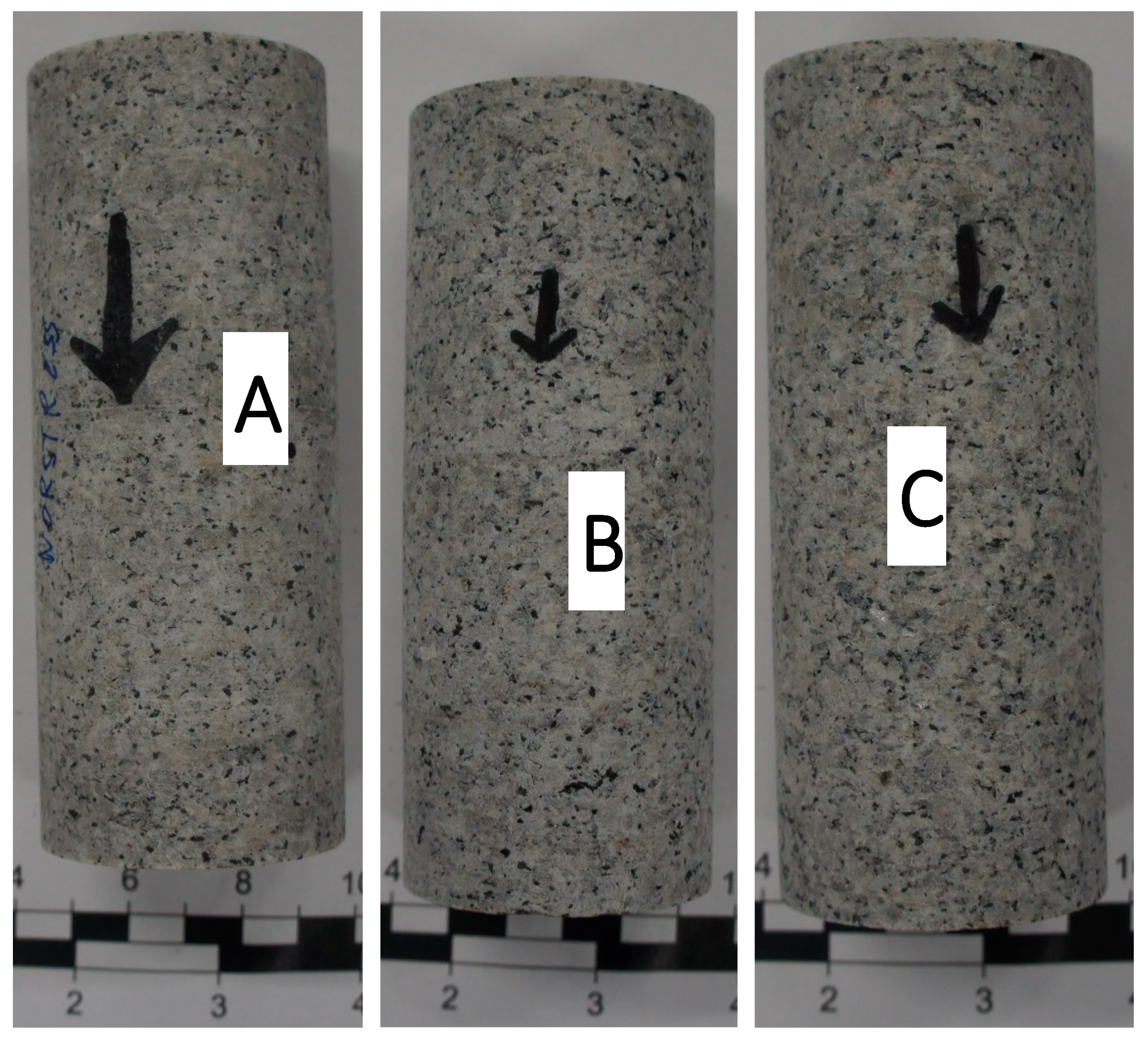


| Sample | Diameter (mm) | Height (mm) | Weight (g) | Density (kg/m3) | Sound Travel Time (ms) | Vp (m/s) | ne (%) | Schmidt Hammer Rn(N) | Converted Rn(L) |
|---|---|---|---|---|---|---|---|---|---|
| A | 48.39 | 124.06 | 598.95 | 2625 | 23.8 | 5213 | 0.44 | 74 | 54 |
| B | 48.35 | 119.21 | 576.50 | 2634 | 24.3 | 4906 | 0.44 | 63 | 45 |
| C | 48.34 | 119.20 | 576.71 | 2636 | 24.2 | 4926 | 0.44 | 63 | 45 |
| Confinement σ3 (MPa) | Peak Strength σ1 (MPa) | ||
|---|---|---|---|
| Sample A | Sample B | Sample C | |
| 0 | 197.7 | 205.8 | 212.8 |
| 2 | 228.1 | 241.5 | 243.7 |
| 5 | 278.2 | 286.9 | 285.5 |
| 10 | 338.3 | 348.8 | 344.1 |
| 15 | 387.8 | 395.0 | 390.2 |
| 20 | 426.3 | 432.5 | 430.7 |
| Sample | “True-UCS” MPa | “Estimated-UCS” (Linear Fitting) | “Estimated-UCS” (Parabolic Fitting) | ||
|---|---|---|---|---|---|
| MPa | Error to the “True-UCS” | MPa | Error to the “True-UCS” | ||
| A | 197.7 | 218.5 | 10.5% | 197.26 | −0.2% |
| B | 205.8 | 233.1 | 11.7% | 210.48 | 2.2% |
| C | 212.8 | 231.2 | 8.0% | 215.47 | 1.3% |
| Sample | “True-UCS” MPa | “Estimated-UCS” (Hoek–Brown Fitting) | |
|---|---|---|---|
| MPa | Error to the “True-UCS” | ||
| A | 197.7 | 201.0 | 1.7% |
| B | 205.8 | 215.6 | 4.8% |
| C | 212.8 | 217.2 | 2.1% |
| Sample | Fitting Equation | Fitting Parameters | ||
|---|---|---|---|---|
| k | σci | |||
| A | 10.89 | 218.49 | ||
| B | 10.56 | 231.12 | ||
| C | 10.34 | 231.24 | ||
| a | b | c | ||
| A | −0.28 | 16.93 | 197.26 | |
| B | −0.27 | 16.44 | 210.48 | |
| C | −0.20 | 14.82 | 215.47 | |
| mi | σci | |||
| A | 32 | 201 | ||
| B | 30 | 216 | ||
| C | 29 | 217 | ||
Disclaimer/Publisher’s Note: The statements, opinions and data contained in all publications are solely those of the individual author(s) and contributor(s) and not of MDPI and/or the editor(s). MDPI and/or the editor(s) disclaim responsibility for any injury to people or property resulting from any ideas, methods, instructions or products referred to in the content. |
© 2025 by the authors. Licensee MDPI, Basel, Switzerland. This article is an open access article distributed under the terms and conditions of the Creative Commons Attribution (CC BY) license (https://creativecommons.org/licenses/by/4.0/).
Share and Cite
Trinh, N.Q.; Grøv, E.; Vistnes, G. A Comparative Study of UCS Results Obtained from Triaxial Tests Under Multiple Failure State Conditions (Test Type II). Appl. Sci. 2025, 15, 3176. https://doi.org/10.3390/app15063176
Trinh NQ, Grøv E, Vistnes G. A Comparative Study of UCS Results Obtained from Triaxial Tests Under Multiple Failure State Conditions (Test Type II). Applied Sciences. 2025; 15(6):3176. https://doi.org/10.3390/app15063176
Chicago/Turabian StyleTrinh, Nghia Quoc, Eivind Grøv, and Gunnar Vistnes. 2025. "A Comparative Study of UCS Results Obtained from Triaxial Tests Under Multiple Failure State Conditions (Test Type II)" Applied Sciences 15, no. 6: 3176. https://doi.org/10.3390/app15063176
APA StyleTrinh, N. Q., Grøv, E., & Vistnes, G. (2025). A Comparative Study of UCS Results Obtained from Triaxial Tests Under Multiple Failure State Conditions (Test Type II). Applied Sciences, 15(6), 3176. https://doi.org/10.3390/app15063176