Structural Reliability Analysis of Aero-Engine Turbine Components Based on Particle Swarm Optimization Back Propagation Neural Network

Abstract

Aero-engine turbine components have complex structures, harsh service load environments, and strong nonlinear structural responses, so it is difficult to establish the explicit limit state function, which is a typical nonlinear implicit function reliability analysis problem. To address this challenge, based on Particle Swarm Optimization and a Back Propagation Neural Network (PSO-BPNN), a reliability analysis approach is proposed in this paper. In the proposed method, the PSO algorithm is employed to optimize the initial weights and biases of the BPNN. This global optimization capability prevents the neural network from falling into local extrema and mitigates overfitting, thus improving the accuracy and generalization of the BPNN in approximating implicit limit state functions. On this basis, the Monte Carlo simulation (MCS) method is used to call the established neural network to calculate the failure probability, and the original implicit limit state function is not needed at this time. The proposed PSO-BPNN approach exhibits higher computational precision and efficiency, particularly for problems with strong nonlinearity and high dimensionality. Numerical examples are used to verify the efficiency and accuracy of the proposed approach, which is further applied to analyze the reliability of an aero-engine turbine casing structure. The results demonstrate that the proposed method not only offers high computational efficiency and accuracy but also provides significant advantages in handling complex nonlinear implicit reliability analysis problems. This indicates its strong potential to serve as a reliable and practical tool for engineering reliability analysis, particularly in the aerospace domain, where structural components often operate under extreme conditions.

1. Introduction

The performance and reliability of the aero-engine significantly influence flight safety. As one of the critical components of an aeroengine, the reliability of the turbine casing plays a vital role in ensuring the healthy operation of the aero-engine [1,2,3]. The high-pressure turbine casing endures extreme loads and operates in a harsh working environment. Consequently, it is essential to investigate the reliability of the high-pressure turbine casing to enhance the safety and reliability of the aero-engine during aircraft operation. In recent years, numerous studies have been conducted to evaluate the reliability and service life of turbine components. In this context, the reliability analysis of turbine components remains a challenging task, given the complexity of their structures, the high dimensionality of input variables, and the strong nonlinearity of responses under severe operating conditions.

In recent years, numerous studies have been conducted to evaluate the reliability and service life of turbine components. For instance, Banaszkiewicz et al. [4] proposed a multi-layered method for assessing steam turbine life, integrating damage calculation, probabilistic analysis, and fracture mechanics. Guan et al. [5] developed a methodology to extend the lifespan of steam turbine rotors by utilizing ultrasonic inspection data for fatigue life assessment while incorporating uncertainties through probabilistic approaches. Despite their contributions, these methods face significant challenges, such as high computational complexity, strong dependency on extensive data, and limited generalizability of the models, particularly for complex structural components in aero-engines. Therefore, efficient and accurate methods are urgently needed to address these limitations and improve the reliability analysis of turbine components.

Structural reliability analysis is based on probability theory, mathematical statistics, and stochastic process theory, which assesses the probability that a structural system can withstand applied loads and environmental impacts while maintaining its functionality within a specified service life under given working conditions. The limit state function of a structure is commonly denoted as G, where G < 0 indicates structural failure. The failure probability can be approximated through numerical methods and is expressed as the frequency of failure sample points among all sample points [6]. The analysis methods primarily consist of numerical methods and approximation methods. Among the numerical methods, the Monte Carlo simulation (MCS) [7] is a widely recognized sampling-based approach that provides high accuracy and reliability in estimating failure probabilities. Failure probability is represented by the ratio of failure sample points to the total number of sample points. Despite its accuracy, MCS becomes computationally prohibitive when large-scale simulations are required, particularly when finite element model calculations are involved. Therefore, variance reduction techniques such as importance sampling (IS) [8] have been proposed to reduce the number of required samples. Nevertheless, IS still demands tens of thousands of sample points to obtain reliable results. Another approach involves employing surrogate model techniques to reduce the computational cost associated with individual sample points in MCS. Rashki et al. [9] proposed an improved MCS method that distributes sample points uniformly in the design space, using the probability density value of sample points as weights to approximate the most probable failure points (MPP) and identify the failure region. This method significantly reduces computational cost while maintaining accuracy, although it still relies on traditional approximate methods for identifying the MPP and failure region. Gallagher et al. [10] introduced a sampling method for model inference and uncertainty quantification, enabling the estimation of parameter distributions and prediction uncertainties. However, this approach still evaluates a large number of sample points in the non-failure region, resulting in low computational efficiency despite its high accuracy.

To address the limitations inherent in numerical methods, approximate methods have been extensively employed in structural reliability. The fundamental principle of these methods lies in substituting the original limit state function with an approximate representation, thereby significantly enhancing computational efficiency. Among these methods, the first-order second moment (FOSM) method [11] and the second-order reliability method (SORM) [12] estimate failure probabilities by expanding the limit state function approximately. Despite their widespread use, these methods face notable challenges when applied to problems involving multiple most probable failure points or pronounced nonlinearity in the vicinity of the failure surface. To overcome such challenges, surrogate models have emerged as an alternative. Commonly used surrogate models include the Kriging model [13,14], polynomial chaos expansion (PCE) [15,16], and response surface methods (RSM) [17,18], which have demonstrated effective performance in addressing these issues. The Kriging model is renowned for its strong local interpolation properties, enabling the prediction of both response values and associated errors at sample points. Leveraging this capability, numerous adaptive Kriging models [19,20,21] have been developed for structural reliability analysis. However, the construction of the Kriging model is computationally intensive for large datasets, and its performance deteriorates in high-dimensional problems. Similarly, the PCE model exhibits strong global interpolation properties but suffers from the “curse of dimensionality”, where computational costs increase exponentially with the number of input variables. To mitigate this, sparse approximation techniques have been proposed, but challenges remain for high-dimensional problems. The RSM is comparatively simpler to construct but frequently lacks accuracy when dealing with complex limit state functions. Consequently, researchers have developed advanced versions of the RSM, such as high-order response surface methods and continuously interpolated high-precision response surface methods. Despite these advancements, the quality and accuracy of the surrogate model largely depend on the sample data, posing challenges in addressing multi-dimensional and high-dimensional problems. While these approaches improve efficiency, they face limitations such as reduced accuracy in highly nonlinear problems, the curse of dimensionality, and high reliance on sample data quality.

With the rapid development of machine learning, the neural network-based surrogate model has demonstrated significant potential in structural reliability analysis. Unlike traditional methods, the neural network model avoids the need to construct complex explicit limit state functions and offers higher accuracy and faster computational speed, particularly when addressing high-dimensional and highly nonlinear problems. Common neural network approaches include the artificial neural network (ANN) [22,23,24] and back propagation neural network (BPNN) [25,26,27]. The ANN model exhibits powerful nonlinear modeling capabilities and adaptability, but its high data requirements and expensive training costs often limit its applicability in certain scenarios. As a significant branch of the ANN, the BPNN model features efficient learning capabilities. By employing an error back propagation algorithm, the BPNN iteratively adjusts weights to minimize errors, thereby optimizing network performance and improving learning efficiency. However, BPNNs face challenges such as susceptibility to local optima, reliance on gradient information, and slow convergence speeds, which can limit their accuracy and efficiency in certain applications.

To address these challenges, Particle Swarm Optimization (PSO) has been proposed as an effective optimization technique. PSO excels at global optimization and does not rely on gradient information, making it well-suited for optimizing BPNN structures. Specifically, PSO can optimize the initial weights and biases of BPNNs, thereby improving convergence speed, mitigating overfitting, and enhancing overall accuracy. The idea of combining PSO with BPNN stems from the need for a more robust and adaptive surrogate model capable of overcoming the limitations of traditional numerical and approximation methods. Building on the results of previous studies and the demonstrated potential of PSO and BPNN, this paper proposes a method that integrates PSO with a BPNN for turbine component analysis.

The proposed PSO-BPNN approach utilizes PSO to optimize the convergence and accuracy of BPNN models, while MCS is employed for failure probability calculation. This integration not only reduces computational costs but also improves the efficiency of addressing high-dimensional and nonlinear reliability problems. The proposed method is validated through numerical and practical engineering examples, with a specific focus on the reliability analysis of an aero-engine high-pressure turbine casing. The results demonstrate the potential of this method to serve as an effective and efficient tool for structural reliability analysis in broader engineering applications.

The remainder of this paper is organized as follows. Section 2 introduces the fundamental principles of structural reliability analysis and key concepts. A brief overview of the PSO-BPNN method is introduced in Section 3, and the application in reliability analysis of the PSO-BPNN method is also elaborated at the same time. Numerical and engineering examples are given in Section 4 to verify the accuracy, efficiency, and engineering applicability of the proposed method. Section 5 discusses the advantages, limitations, and potential improvements of the proposed PSO-BPNN method. Finally, Section 6 presents the conclusions of this paper.

2. The Principle of Structural Reliability Analysis

The importance of structural reliability lies in ensuring long-term functionality, operational safety, and cost-effective maintenance. Proactively addressing structural reliability significantly reduces risks, prevents early defects or failures, and minimizes the likelihood of catastrophic events throughout a structure’s service life. Furthermore, achieving high reliability ensures that structures meet their intended functions while reducing long-term maintenance costs. This approach is particularly critical in fields such as aerospace, civil engineering, and energy systems, where structural failures can result in severe consequences.

2.1. The Limit State of the Structure

To accurately describe the working state of a structure in the analysis and design of structural reliability, a clear definition of the boundaries between structural safety, durability, functionality, and failure is required. These boundaries are collectively referred to as the limit state of the structure. The limit state is defined as the specific condition beyond which the entire structure, or a part of it, can no longer meet the functional requirements specified in the design. This specific condition is mathematically represented by the limit state function.

The limit state of a structure essentially represents the critical transition point between its functional and failed states. When this value is exceeded, the structure is considered to be in an unsafe, non-durable, or inapplicable state. Conversely, if this value is not exceeded, the structure remains in a safe, durable, and applicable state. Let the basic random variables of the structure be represented by the random vector $\mathit{X}=(X_1,X_2,\dots ,X_n)$. The function that describes the working state of the structure can then be expressed as Equation (1), referred to as the limit state function.

$$Y=g(\mathit{X})$$

(1)

Then, the working state of the structure can be shown by Equation (2).

$$Y=g(\mathit{X})\left\{\begin{array}{c}<0\hspace{1em}\hspace{1em}failure state\\ =0\hspace{1em}\hspace{1em} limit state\\ >0\hspace{1em}\hspace{1em}reliable stat\mathrm{e}\end{array}\right.$$

(2)

The limit state of a structure can be defined either objectively based on the actual condition of the component or subjectively by experts, who take into account experience, specific requirements, and human control factors.

2.2. Degree of Reliability for Structure

In the current unified standards for structural reliability design, structural reliability is defined as the ability of structural components to fulfill predetermined functions within a specified time frame and under specified conditions. Furthermore, structural reliability is quantitatively described as the probability of successfully completing these functions within the given time and conditions. Thus, structural reliability can be regarded as a probabilistic measure of a structure’s performance. Under the influence of various random factors, the capability of a structural system to perform its specified functions can be more accurately assessed when it is expressed in terms of probability.

Let $P_s$ denote the probability that the structure successfully completes its predetermined function within the specified time and conditions. This probability $P_s$ represents the reliability of the structure. Conversely, the probability that the structure fails to complete the predetermined function is referred to as the failure probability, denoted as $P_f$. Since reliability and failure are two mutually exclusive events, the reliability and failure probabilities are complementary, and this relationship can be expressed by Equation (3).

$$P_f+P_s=1$$

(3)

According to the definition of structural reliability and the basic principles of probability theory, if the random vector composed of the basic random variables of the structure is denoted as $\mathit{X}=(X_1,X_2,\dots ,X_n)$, the corresponding joint probability density function as $f_X(\mathit{x})$, and the limit state function represented by this random vector as $Y=g(\mathit{X})$, then the failure probability of the structure can be expressed as shown in Equation (4).

$$P_f=P(Y<0)={{\displaystyle \int }}_F{f}_X(\mathit{x})\mathrm{d}\mathit{x}$$

(4)

where $F=\left\{\mathit{x}\right|g(\mathit{x})\le 0\}$ represents the failure domain of the structure.

If the structure has two independent random variables, R and S, with their corresponding probability density functions denoted as $f_R(r)$ and $f_S(s)$, and their probability distribution functions represented as $F_R(r)$ and $F_S(s)$, respectively, the structural limit state function can be expressed as shown in Equation (5).

$$Y=g(R,S)=R-S$$

(5)

Then, the failure probability of the structure can be expressed using Equation (6).

$$P=P(Y<0)={\int }_0^{+\infty }[{\int }_0^s{f}_R(r)\mathrm{d}r]f_S(s)\mathrm{d}\mathrm{s}={\int }_0^{+\infty }{F}_R(s)f_S(s)\mathrm{d}\mathrm{s}$$

(6)

In the analysis of structural reliability, R is generally used to represent the resistance of the structure, while S represents the effect of the action on the structure. The resistance R can either be a single basic random variable or a comprehensive random variable represented by several basic random variables. In practical structural analysis, there are often numerous random variables, and moreover, the limit state function may be nonlinear, making the problem relatively complex. As a result, solving the failure probability through numerical integration becomes very difficult, or even impossible, in such cases. To address this challenge, the concept of the reliability index $\beta$ is introduced.

Assuming that R and S both follow a normal distribution, their means and standard deviations are ${\mu }_R$, ${\mu }_S$, ${\sigma }_R$, and ${\sigma }_S$, respectively. Then, the limit state function $Y=R-S$ also follows a normal distribution, with its mean and standard deviation denoted as ${\displaystyle \frac{{\mu }_S+{\mu }_S}{2}}$ and ${\sigma }_Y=\sqrt{{\sigma }_R^2+{\sigma }_S^2}$, respectively. The probability of $Y<0$ is referred to as the failure probability. At this point, the failure probability of the structure can be expressed as shown in Equation (7).

$$P_f=P(Y<0)=F_Y(0)={\int }_{-\infty }^0{\displaystyle \frac{1}{\sqrt{2\pi }{\sigma }_Y}}\exp [-{\displaystyle \frac{{(Y-{\mu }_Y)}^2}{2{\sigma }_Y^2}}]\mathrm{d}Y$$

(7)

The reliability index and the failure probability can be converted using Equation (8).

$$\beta =-{\Phi }^{-1}(P_f)$$

(8)

where ${\Phi }^{-1}\left(•\right)$ is the inverse cumulative distribution function (CDF) of the standard normal distribution.

Due to the complexity of structures, it is generally difficult to define the explicit limit state function. The surrogate model method is an effective approach to address such challenges. This method uses a finite number of structural analysis results to fit an explicit expression, which approximately replaces the unknown limit state function for reliability index calculation. However, commonly used surrogate models, such as the Kriging model, PCE model, and RSM model, often struggle to handle scenarios with multiple inputs or high-dimensional problems.

To overcome these limitations, a particle swarm optimization–back propagation neural network (PSO-BPNN) method for reliability analysis is proposed. This method trains a neural network using a finite number of structural analysis results, enabling it to serve as an approximate replacement for the implicit limit state function in reliability index calculations.

3. Reliability Analysis Method Based on PSO-BPNN

3.1. Back Propagation Neural Network

The BPNN is a multilayer, fully connected feedforward artificial neural network trained using the error back propagation algorithm. The error backpropagation algorithm used in the BPNN is a supervised neural network training algorithm characterized by its simple structure, strong nonlinear approximation capability, and self-learning and self-adaptive features [28,29]. A large amount of data generated through ANSYS 2022R1 finite element analysis software can be used as sample data. The error back propagation algorithm is employed to calculate the weights of the neuron connections, thereby establishing an optimized neural network model capable of accurately representing the input–output relationships.

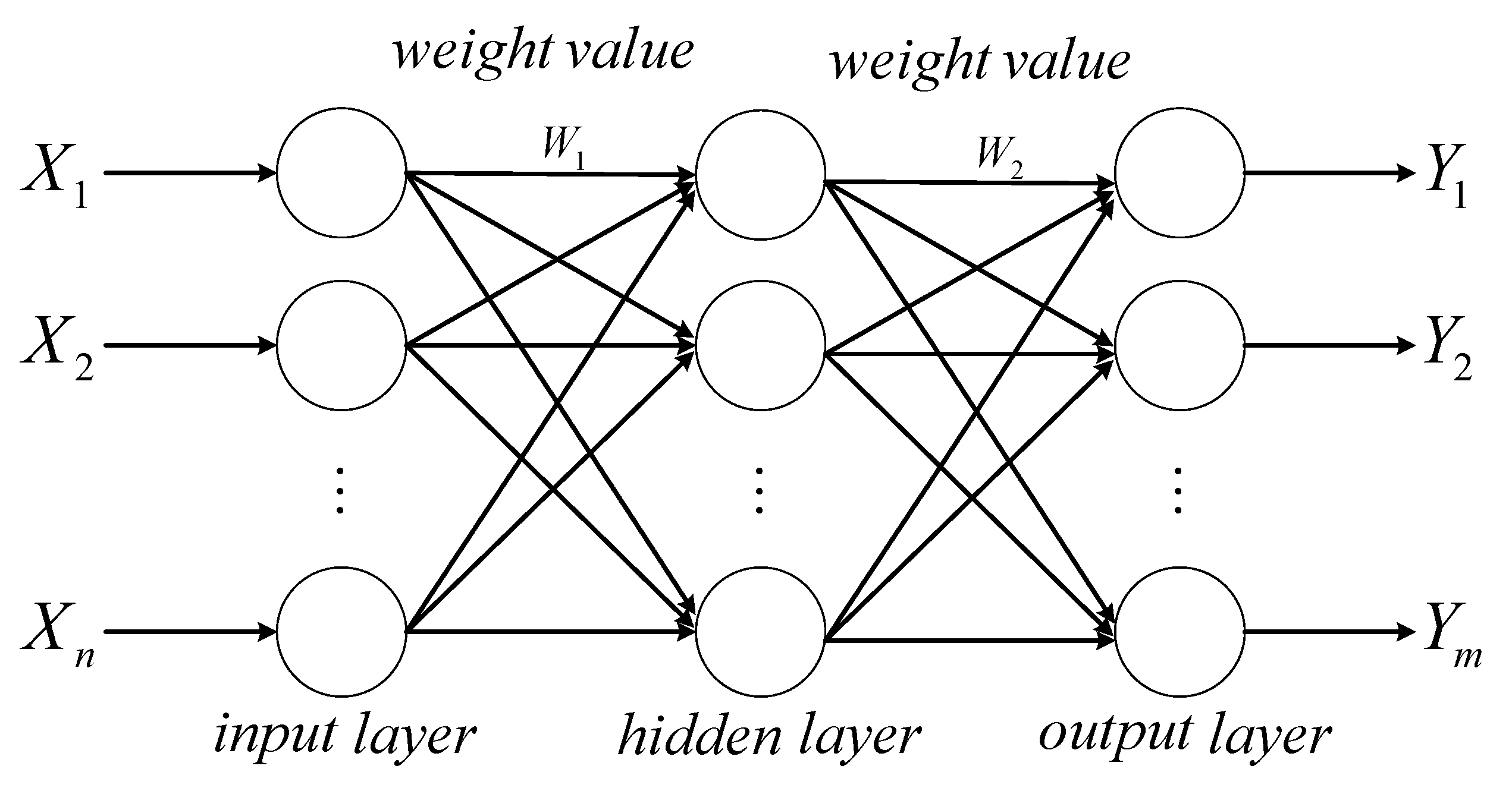
The neural network structure is designed with n input nodes, l hidden layer nodes, and m output nodes, as shown in Figure 1. A BPNN with one hidden layer and a continuous activation function can theoretically approximate any nonlinear continuous function. The hidden layer employs the sigmoid activation function “tansig”, while the output layer uses the linear activation function “purelin”. The network’s learning algorithm is based on the Levenberg–Marquardt algorithm.

The BPNN is trained using a large number of samples $(\mathit{X},\mathit{Y})$, with the weights $(W_1,W_2)$ and biases $(B_1,B_2)$ continuously adjusted via the network’s adaptive algorithm. The training process aims to minimize the mean squared error (MSE) of the objective function, thereby accurately capturing the input–output relationship. However, a major limitation of the BPNN is its susceptibility to becoming trapped in local extrema. This limitation arises from the fact that no additional parameters are introduced during the training process, and the algorithm solely relies on adjusting the initial weights and biases based on the training samples. As a result, the performance of the model is highly sensitive to the initial values of these parameters. If the weights and biases are initialized randomly, there is a considerable risk that the MSE optimization process will converge to a local extremum, leading to suboptimal weight and bias values. Consequently, this issue may cause the trained network to produce inaccurate predictions, negatively impacting its reliability and generalization capability.

3.2. PSO-BPNN Method

PSO is a population-based optimization algorithm inspired by the social and behavioral characteristics of biological systems. It is designed to solve complex optimization problems by iteratively improving candidate solutions based on a predefined fitness function. PSO has significant advantages, such as its ability to escape local extrema and its strong capability for finding global optima [30].

In the PSO algorithm, the objective function is referred to as the fitness function, which evaluates the quality of each candidate solution. Each particle within the search space is characterized by its position and velocity, and its fitness value is determined by the fitness function. The particles iteratively update their positions and velocities by comparing their personal best fitness value (individual best) with the global best fitness value (shared among the swarm). Through this process of interaction and adjustment, the particle population converges to the optimal value of the fitness function, thereby achieving optimization of the objective function [31].

The predefined fitness function in this study is shown in Equation (9).

$$\mathrm{fit}\left(x\right)={\displaystyle \frac{1}{c+1+Y+my}}$$

(9)

where $c$ is the estimated value of the limit state function $Y=g\left(\mathit{X}\right)$; $y$ is the penalty term, representing the degree of constraint violation; $m$ is the penalty coefficient, controlling the weight of the penalty term.

The fitness function was designed to fulfill two main objectives: (1) minimize the unreliability by reducing the value of $c$, and (2) penalize solutions that violate physical or operational constraints. The term ${\displaystyle \frac{1}{c+1}}$ ensures that particles closer to the failure threshold receive lower fitness values, encouraging the search toward safer and more reliable solutions. Meanwhile, the penalty term $Y$ and its coefficient $m$ are crucial for guiding the optimization process toward feasible regions of the design space. The value of $m$ was determined through a sensitivity analysis to balance constraint satisfaction and algorithm convergence, ensuring that the penalty neither overwhelms the optimization process nor allows infeasible solutions to persist.

The choice of this fitness function is crucial for achieving effective optimization within the PSO-BPNN framework. As the PSO algorithm iteratively adjusts the particles’ positions and velocities, the fitness function plays a central role in evaluating the quality of each candidate solution. By minimizing the fitness value, the PSO algorithm optimizes the neural network’s parameters, improving its ability to approximate the implicit limit state function and predict failure probabilities accurately.

The PSO-BPNN method integrates PSO with the BPNN by treating the weights and biases of the neural network as particles within the swarm. PSO is employed to optimize these particles by iteratively updating their positions (the weights and biases) and velocities according to a predefined fitness function. The fitness function evaluates the performance of the neural network, aiming to minimize the error of the neural network. Through this process, the PSO-BPNN method seeks to identify the optimal set of weights and biases that enhance the accuracy and generalization capability of the BPNN. This ultimately establishes a more precise input–output relationship, thus improving the network’s overall predictive performance.

In the standard PSO algorithm, the particle swarm is composed of $\mathit{N}=(N_1,N_2,N_3,\dots ,N_n)$ particles. The position of the ith particle is represented by ${\mathit{x}}_{\mathit{i}}=(x_{i1},x_{i2},x_{i3},\dots ,x_{id})$, and its velocity is denoted as ${\mathit{v}}_{\mathit{i}}=(v_{i1},v_{i2},v_{i3},\dots ,v_{id})$. At the tth iteration, the velocity and position of the particle are updated for the (t + 1)th iteration according to Equations (10) and (11).

$${\mathit{x}}_{\mathit{i}}^{t+1}={\mathit{x}}_{\mathit{i}}^t+{\mathit{v}}_{\mathit{i}}^{t+1}$$

(10)

$${\mathit{v}}_{\mathit{i}}^{t+1}=w{\mathit{v}}_{\mathit{i}}^t+c_1{r}_1\left(P_{i\mathrm{best}}^t-{\mathit{x}}_{\mathit{i}}^t\right)+c_2{r}_2\left(G_{\mathrm{best}}^t-{\mathit{x}}_{\mathit{i}}^t\right)$$

(11)

where $w{v}_i^t$ is the inertial term of particle motion; $w$ is inertia weight; $c_1{r}_1(P_{i\mathrm{best}}^t-x_i^t)$ is the individual confidence term; $c_1$ is the acceleration factor, generally non-negative constant; $P_{i\mathrm{best}}^t$ is the individual extreme point; $r_1$ is a random number, where the value range is $[0,1]$; $c_2{r}_2(G_{\mathrm{best}}^t-x_i^t)$ is the group extreme point; $c_2$ is the acceleration factor, generally non-negative constant; $r_2$ is a random number, where the value range is $[0,1]$.

The steps of the PSO-BPNN method are outlined as follows:

(1)

Generate the initial population adaptively based on random variables.

(2)

Obtain the objective function. It is the functional equation fitted by the BPNN.

(3)

Determine the fitness function based on the minimum value of the search objective and calculate the fitness result, as shown in Equation (9).

(4)

Update the position, velocity, and inertia weight of the particles, and obtain the fitness function value through each iteration.

(5)

End when the result meets the convergence condition; if the convergence condition is not met, repeat steps 3 and 4 until the condition is satisfied.

To ensure that the output of the BPNN accurately approximates the behavioral characteristics of the target function, this paper employs the PSO algorithm to perform a global optimization of the network’s weight and bias parameters. Given that the PSO algorithm significantly enhances the stability and convergence performance of neural networks in practical applications, a surrogate relationship is established between the trained neural network and the target limit state function, as expressed in Equation (12).

$$\overline{g}(\mathit{X})\approx g(\mathit{X})$$

(12)

where $\overline{g}(\mathit{X})$ represents the limit state function approximated by the neural network, which has been optimized using the PSO algorithm, and $g(\mathit{X})$ denotes the target limit state function.

3.3. Failure Probability Calculation Process Based on the PSO-BPNN Method

This paper proposes a method for structural reliability analysis that integrates the particle swarm optimization back propagation neural network to calculate failure probability. By employing the PSO-BPNN method, it addresses the limitations of the traditional MCS, such as high computational cost and slow convergence rate.

The core concept of the traditional MCS method is to approximate the population mean using the sample mean when the sample size is sufficiently large. The fitted limit state function $\overline{g}(\mathit{X})$ divides the input variable space into the failure domain $F=\left\{\mathit{x}\right|g(\mathit{x})\le 0\}$ and the safe domain $\mathrm{S}=\left\{\mathit{x}\right|g(\mathit{x})>0\}$. To distinguish between failure and safe states in structural reliability analysis, a failure domain indicator function $I_F\left({\mathit{x}}_j\right)$ is introduced. If $\overline{g}(\mathit{X})\le 0$, then $I_F({\mathit{x}}_j)=1$; otherwise, $I_F({\mathit{x}}_j)=0$. The MCS method generates N samples of input variables based on their joint probability density function. The sample failure probability is then calculated, as shown in Equation (13), as the ratio of the number of samples m falling within the failure domain to the total number of samples N.

$${\widehat{P}}_f={\displaystyle \frac{1}{N}}\sum _{j=1}^N{I}_F\left({\mathit{x}}_j\right)={\displaystyle \frac{m}{N}}$$

(13)

The MCS method is straightforward to implement, and its accuracy converges to the true solution as the sample size increases. However, in practical engineering applications, the structural limit state function is often highly complex or even implicit, such as a finite element model. Evaluating the limit state function for each sample to compute response values involves considerable computational cost. To address this issue, the method proposed in this paper is designed to overcome the computational challenges associated with the MCS method in structural reliability analysis. By introducing a substitution of limit state function, the computational burden of repeatedly evaluating the limit state function can be significantly reduced. Specifically, a neural network is trained to approximate the functional relationship of the limit state function, thereby eliminating the need to directly evaluate the original function. The detailed steps are as follows:

(1)

Collection and preprocessing of sample data.

In this step, the Latin Hypercube Sampling (LHS) method is used to generate K sets of input data by sampling the random variables $\mathit{X}=\{X_1,X_2,\dots ,X_n\}$. For each input sample, the performance response is calculated, and the corresponding limit state function $g(\mathit{X})$ is evaluated to obtain K sets of output results. To ensure numerical stability and prevent data with small magnitudes from being annihilated during computation, it is essential to normalize all input and output parameters. Since the activation function used between the input layer and the hidden layer is an S-shaped function, the data are normalized and mapped to the [0, 1] interval. This ensures compatibility with the activation function and facilitates better con-vergence during training. The mapping function for normalization is provided in Equation (14):

$$x_{\mathrm{st}}={\displaystyle \frac{x-x_{\min }}{x_{\max }-x_{\min }}}$$

(14)

where $x_{\mathrm{st}}$ represents the normalized data; $x$ denotes the original data; $x_{\max }$ and $x_{\min }$ correspond to the maximum and minimum values of the original dataset for each parameter, respectively.

(2)

Determine the structure of the BPNN.

The structure of BPNN is defined employing $\mathit{X}=\{X_1,X_2,\dots ,X_n\}$ as the system input and $g(\mathit{X})$ as the output variable.

(3)

Split dataset.

Divide the dataset into a training set and a testing set, where 80% of the sample data are allocated to the training set, while the remaining 20% are used as the testing set. This division is a critical step in effectively training the BPNN, as it helps mitigate the risk of overfitting and ensures the model exhibits strong generalization capability.

(4)

Configurate training parameters.

Prior to training the BPNN, the training parameters must be appropriately configured. Specifically, the learning rate is set to 0.01, the maximum number of training iterations is set to 1000, and other parameters are maintained at their default values. These configurations are designed to balance training efficiency and effectiveness. They ensure that it converges to a satisfactory solution without incurring excessively long training times or encountering issues such as infinite loops.

(5)

Use the PSO algorithm to optimize neural network.

The initial connection weights and thresholds of the BPNN are selected as the target parameters for optimization using the PSO algorithm. Through the iterative optimization process of the PSO algorithm, the optimal initial connection weights and thresholds are determined once the convergence condition (the maximum number of iterations, $\max gen=50$) is satisfied. The parameters corresponding to the optimal particle are then assigned to the weight and threshold parameters within the network structure of the BPNN. Subsequently, the neural network is executed and trained to develop the optimal model.

(6)

Model validation.

After completing the model training, the performance of the model is evaluated using the test set samples. If the goodness of fit satisfies the convergence condition ($R^2\ge 99\%$), the process is considered complete. Otherwise, the sample size K is increased, and steps 1–5 are repeated until the convergence condition is fulfilled. Finally, the network model that meets the specified requirements is obtained and output.

(7)

Calculate failure probability.

The MCS method is employed for failure probability calculation. A total of N samples are generated for each of the random input variables $\mathit{X}=\{X_1,X_2,\dots ,X_n\}$. In this study, the LHS method is employed for generating random samples, as it improves sampling efficiency and ensures better coverage of the input variable distributions compared to simple random sampling. Once the samples are generated, the next step involves evaluating the limit state function for each sample. The optimal PSO-BPNN model obtained in step 5 is then used to evaluate the corresponding limit state function values $\overline{g}(\mathit{X})$. The trained PSO-BPNN serves as a surrogate model, significantly reducing computational costs compared to directly evaluating the finite element model. Subsequently, the failure probability estimate ${\widehat{P}}_f$ is determined using Equation (13).

The algorithm flowchart is shown in Figure 2.

This approach leverages the computational efficiency of the PSO-BPNN model and the robustness of the MCS method to provide accurate failure probability estimates. The integration of the LHS technique ensures that the stochastic space of the input variables is thoroughly explored, improving the reliability of the results.

4. Example

4.1. Nonlinear Limit State Function

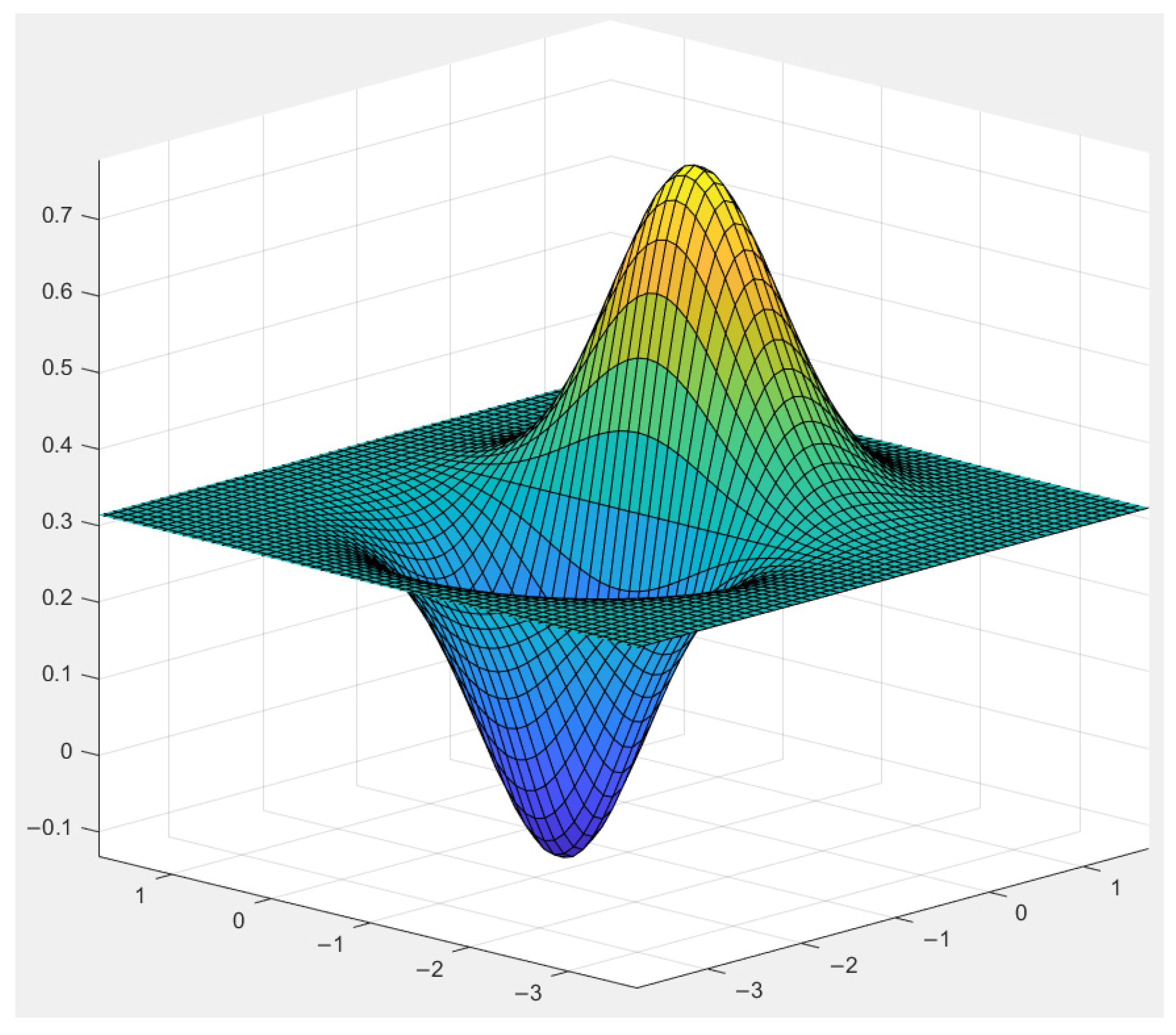
Consider the functional form as shown in Equation (15):

$$Y=g(\mathit{X})=X_1\exp (-X_1^2-X_2^2)+0.414$$

(15)

where $X_i(i=1,2)~N(0,1)$ are independent of each other.

The relationship between the input variables and the output response of the functional form is illustrated in Figure 3, which demonstrates a high degree of nonlinearity.

To demonstrate the computational performance of the PSO-BPNN method in effectively handling a highly nonlinear limit state function, the failure probability was calculated for the same example using both the MCS method and the PSO-BPNN method. The cumulative sample size required for the MCS method was $1\times {10}^5$, whereas the PSO-BPNN method required only $2\times {10}^3$ samples. A comparison of the computational results obtained from the two methods is presented in

Table 1. Failure probability calculated by two methods.

Method	$\mathbf{Failure} \mathbf{Probability} {\mathbf{P}}_{\mathit{f}}$	$\mathbf{Number} \mathbf{o}\mathbf{f} \mathbf{S}\mathbf{a}\mathbf{m}\mathbf{p}\mathbf{l}\mathbf{e}\mathbf{s} \mathit{N}$	$\mathbf{Error}$
MCS	$9.667\times {10}^{-3}$	$1\times {10}^5$	-
Proposed	$9.958\times {10}^{-3}$	$2\times {10}^3$	2.92%

, highlighting the efficiency and accuracy of the PSO-BPNN method relative to the MCS method.

4.2. The Limit State Function with High-Dimensional Variables

Consider the functional form as shown in Equation (16):

$$Y=g(\mathit{X})={\displaystyle \frac{\left(X_1^2+8\right)\left(X_2-0.5\right)}{20}}+{\displaystyle \sum _{i=1}^{20}{X}_i}{X}_{i+1}-15$$

(16)

where $X_i(i=1,2,\dots 20)~N(1,1.5)$ are independent of each other. The limit state function incorporates 20 random variables, classifying it as a high-dimensional reliability analysis problem.

To demonstrate the computational performance of the PSO-BPNN method in addressing a high-dimensional limit state function, the failure probability for the same example was calculated using both the MCS method and the PSO-BPNN method. The cumulative sample size for the MCS method was significantly larger, whereas the PSO-BPNN method required only $1.5\times {10}^3$ samples. A comparison of the computational results obtained using the two methods is presented in

Table 2. Failure probability calculated by two methods.

Method	$\mathbf{Failure} \mathbf{Probability} {\mathbf{P}}_{\mathit{f}}$	$\mathbf{Number} \mathbf{o}\mathbf{f} \mathbf{S}\mathbf{a}\mathbf{m}\mathbf{p}\mathbf{l}\mathbf{e}\mathbf{s} \mathit{N}$	$\mathbf{Error}$
MCS	$1.8619\times {10}^{-2}$	$1\times {10}^5$	-
Proposed	$1.7913\times {10}^{-2}$	$1.5\times {10}^3$	3.79%

. The findings demonstrate that the PSO-BPNN method achieves superior computational accuracy while significantly reducing the required sample size.

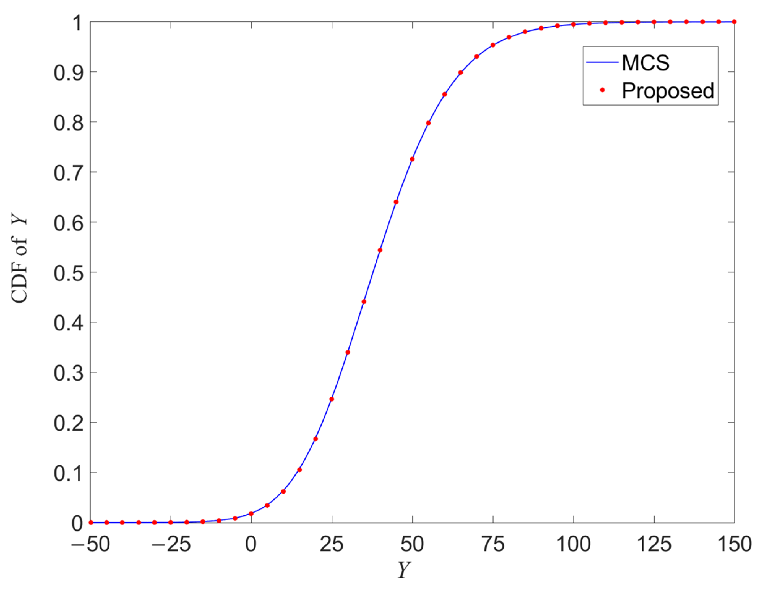
The cumulative distribution function (CDF) of the output Y obtained using the two methods is presented in Figure 4. As shown in the figure, the CDF curves produced by the two methods are nearly identical across the entire range. This observation further validates the accuracy and efficiency of the proposed method in managing a high-dimensional limit state function.

4.3. Structure of the Aero-Engine Turbine Casing

In this section, reliability analysis of the aero-engine turbine casing is used as an example. The failure probability is calculated using the PSO-BPNN method to validate the engineering feasibility and practical applicability of the proposed method.

The turbine casing functions as the foundation for the entire turbofan engine. Most turbine casings are thin-walled welded structures featuring localized structural characteristics, such as weld seams and transition fillets. These regions often display abrupt geometric changes, leading to stress concentrations and an increased risk of failure under loading conditions. The occurrence of a crack in these areas could critically compromise the flight safety of the aircraft. In this paper, a reliability analysis is performed on the turbine casing structure of a specific type of turbofan engine. ANSYS finite element software is employed to develop a stress–response relationship model for the turbine casing structure.

(1)

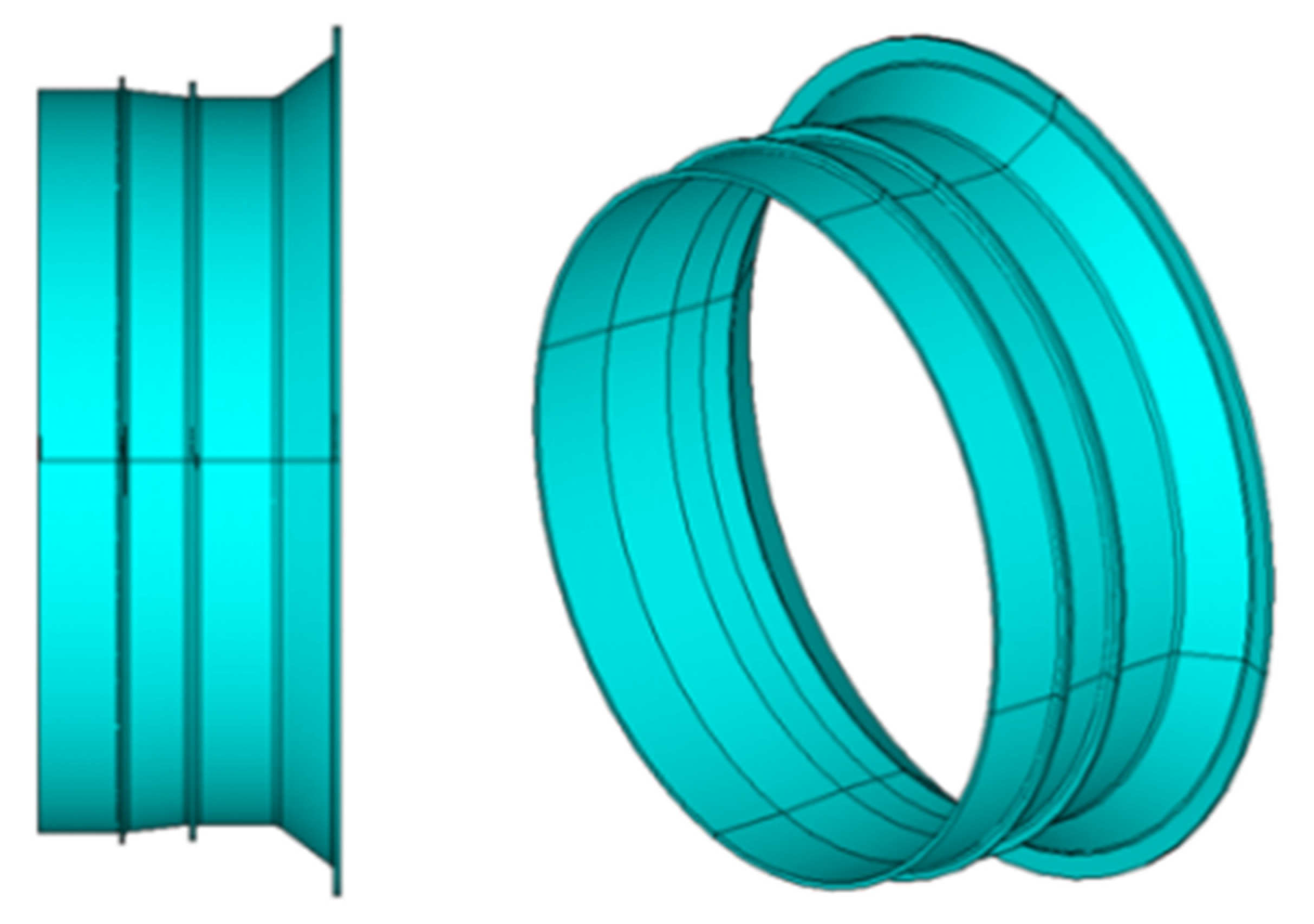
Simplified geometric modeling of the turbine casing.

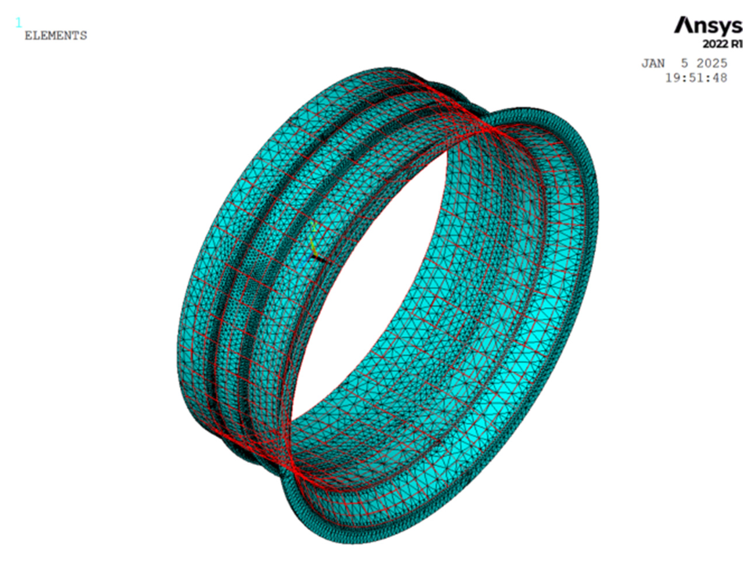
For the geometric modeling and material property definition of a certain type of turbofan engine turbine casing, the influence of the support on the mounting edge is ignored, simplifying it into an axisymmetric model. The stiffening ribs on the outer surface of the turbine casing are considered, and the mounting holes on the mounting edge of the turbine casing are appropriately simplified. The simplified turbine casing model is shown in Figure 5.

(2)

Load and constraint application.

During engine operation, stages such as startup, shutdown, and working condition transitions occur. These result in changes in internal gas temperature, which induce thermal stress in the structure. The turbine casing is subjected to the combined effects of mechanical stress and thermal stress, necessitating a thermo-mechanical coupling analysis. Considering that one-way coupling analysis is more efficient and can maintain an adequate level of accuracy for relatively simple structural problems, this paper employs the one-way coupling method to perform the thermo-mechanical coupling analysis on the turbine casing.

The internal–external pressure difference (ΔP) is the primary load responsible for the mechanical stress in the turbine casing, contributing approximately 90% of the total stress level. Therefore, in the thermo-mechanical coupling analysis, the mechanical load is simplified to only account for the internal–external pressure difference. The load spectrum of the turbine casing is depicted in Figure 6. The boundary condition is defined as a fixed support applied at the rear mounting edge of the turbine casing, as illustrated in Figure 7.

The application of mechanical loads and boundary conditions on the turbine casing structure is illustrated in Figure 8.

In this study, six random variables are considered, including the material yield strength ${\sigma }_{P0.1}(\mathrm{MPa})$, elastic modulus $E(\mathrm{GPa})$, Poisson’s ratio $\mu$, linear expansion coefficient $\alpha ({10}^{-6}/°\mathrm{C})$, external pressure $P_1(\mathrm{MPa})$, and internal pressure $P_2(\mathrm{MPa})$. These variables are treated as random inputs to capture their inherent uncertainties, while other parameters are treated as deterministic. The random treatment of these variables ensures that the reliability analysis reflects the variability and uncertainties present in real-world operating conditions. The range of variations for these variables is specified in

Table 3. Distribution type and parameters of random variables.

Variables	Distribution Type	Mean Value	Standard Deviation
${\sigma }_{P0.1}$	Normal	550	55
$E$	Normal	170	24.3
$\mu$	Normal	0.3	0.03
$\alpha$	Normal	1.44	0.144
$P_1$	Normal	0.1	0.01
$P_2$	Normal	1.6	0.16

, covering distribution type, mean value, and standard deviation to ensure the reliability analysis is representative of actual operating conditions.

Based on the strength failure criterion of the turbine casing structure, the limit state function is defined as shown in Equation (17):

$$Y=g(\mathit{X})={\sigma }_{P0.1}-{\sigma }_{\max }(E, \mu , \alpha , P_1, P_2)$$

(17)

where ${\sigma }_{\max }(E, \mu , \alpha , P_1, P_2)$ represents the maximum stress function of the turbine casing, which is characterized as an implicit limit state function and can be obtained through finite element analysis.

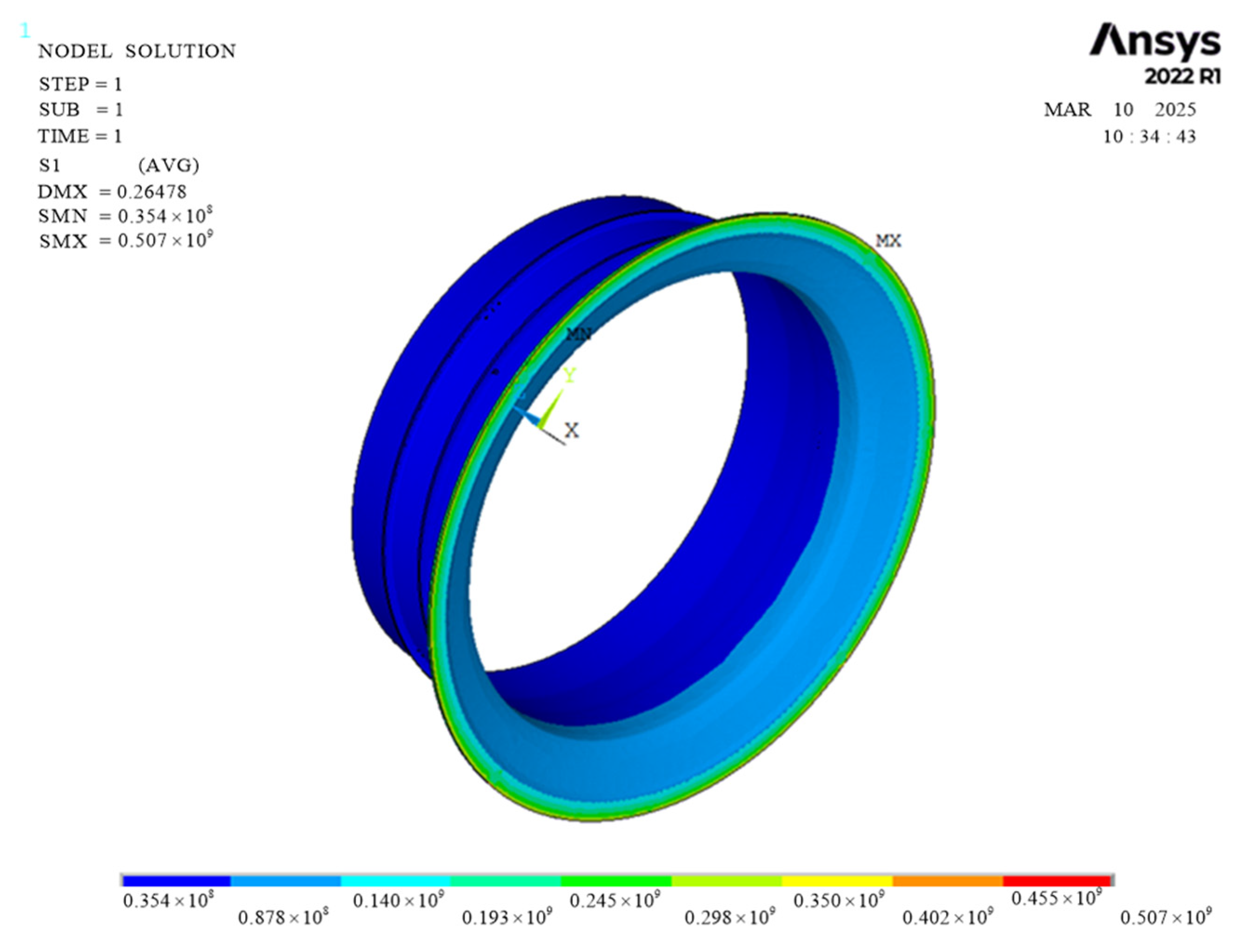
The stress contour diagram of the casing structure, corresponding to the mean values of the random variables $E$, $\mu$, $\alpha$, $P_1$, and $P_2$ is illustrated in Figure 9.

In the context of the PSO-BPNN framework, random variables $E, \mu , \alpha , P_1$, and $P_2$ serve as the inputs to the model. They represent the key factors influencing the structural reliability of the turbine casing. The output of the PSO-BPNN model is the maximum stress ${\sigma }_{\max }(E, \mu , \alpha , P_1, P_2)$.

The limit state function in this example is implicit, requiring finite element analysis to obtain the corresponding response outputs. The traditional MCS approach involves double-layer sampling, necessitating numerous calls to the finite element model. This leads to significant computational costs and excessive time consumption, making it impractical for engineering applications. To address this issue, the PSO-BPNN method proposed in this paper is employed to efficiently compute the failure probability.

The calculation results are presented in

Table 4. Failure probability calculated by PSO-BPNN method.

Method	$\mathbf{Failure} \mathbf{P}\mathbf{r}\mathbf{o}\mathbf{b}\mathbf{a}\mathbf{b}\mathbf{i}\mathbf{l}\mathbf{i}\mathbf{t}\mathbf{y} {\mathbf{P}}_{\mathit{f}}$	$\mathbf{Number} \mathbf{o}\mathbf{f} \mathbf{S}\mathbf{a}\mathbf{m}\mathbf{p}\mathbf{l}\mathbf{e}\mathbf{s} \mathit{K}$	${\mathit{R}}^2$
Proposed	$2.43\times {10}^{-3}$	1000	99.993%

. In this example, when the sample size K = 1000, the constructed neural network model demonstrates a high goodness of fit ($R^2=99.993\%$), indicating that the selected independent variables explain approximately 99.993% of the variance in the dependent variable. This outcome verifies the strong correlation between the independent and dependent variables, establishing a solid foundation for further practical applications and confirming the effectiveness and accuracy of the network model. The failure probability calculated using the PSO-BPNN method is $2.43\times {10}^{-3}$, highlighting the engineering practicality and reliability of the proposed algorithm.

5. Discussion

The results presented in Section 4 demonstrate the efficiency and accuracy of the proposed PSO-BPNN-based reliability analysis approach. To further justify these findings and validate the effectiveness of the proposed method, a detailed discussion is provided below:

(1)

Comparison with existing methods.

Compared to traditional reliability analysis methods, the proposed PSO-BPNN approach demonstrates significant advantages. Traditional methods often face challenges when dealing with complex nonlinear implicit functions, primarily due to their limitations in capturing global optimization solutions and their susceptibility to overfitting. In contrast, the PSO-BPNN method utilizes the global optimization capability of the PSO algorithm to optimize the weights and biases of the BPNN. This enhances the neural network’s ability to approximate complex implicit limit state functions while effectively avoiding local extrema. Furthermore, the integration of the MCS method ensures robust and accurate estimation of failure probabilities.

(2)

Efficiency and computational cost.

Numerical results reveal that the proposed method achieves a high level of computational efficiency. For example, in the face of high nonlinearity or high-dimensional situations, the computational time was significantly reduced compared to conventional methods, all while maintaining accuracy. This improvement in computational efficiency can be attributed to the optimized neural network training process.

(3)

Improvements in accuracy.

The accuracy of the proposed approach has been validated through numerical examples, with results closely aligning with benchmark solutions obtained using traditional methods. The integration of PSO ensured that the neural network effectively avoided overfitting, a common challenge in reliability analysis when employing machine learning models.

(4)

Advantages in practical applications.

The practical utility of the proposed method was demonstrated in the reliability analysis of an aero-engine turbine structure, a complex engineering problem characterized by pronounced nonlinearities. The results confirm that the method effectively addresses the challenges posed by such real-world applications, providing accurate and reliable outcomes. This highlights its potential as a valuable tool for engineering reliability assessments, especially in aerospace engineering, where implicit nonlinear functions are prevalent.

(5)

Limitations and future directions.

Although the proposed approach performed well in the presented examples, further research is required to evaluate its scalability for even more complex systems. Additionally, the integration of adaptive sampling techniques into the PSO-BPNN framework could further improve its computational efficiency. Future work could also focus on comparing the proposed method with other advanced machine learning-based approaches to better understand its relative performance and potential advantages.

In conclusion, the proposed PSO-BPNN-based reliability analysis approach features both accuracy and efficiency, while offering substantial advantages in addressing complex nonlinear implicit reliability problems in engineering applications.

6. Conclusions

In order to solve the challenges in calculating failure probabilities arising from the highly nonlinear, high-dimensional, and implicit characteristics of the limit state function in reliability analysis, this paper proposes a novel structural reliability analysis method that integrates PSO with the BPNN. In the proposed method, the PSO algorithm is introduced to optimize the BPNN model, effectively mitigating overfitting issues and improving processing accuracy and convergence speed.

Numerical results demonstrate that the proposed method achieves a relatively small prediction error for failure probabilities while significantly reducing computational cost compared to MCS. This illustrates the method’s reliable computational accuracy and stability, even when applied to limit state functions characterized by high nonlinearity and dimensionality. In the practical case of an aero-engine turbine casing, the PSO-BPNN method demonstrated both efficiency and robustness in addressing complex engineering challenges. These results underscore the method’s strong potential for broader applications across various engineering disciplines.

Nevertheless, further research is critical to improving the scalability and adaptability of the proposed method. One promising direction lies in integrating adaptive sampling techniques into the PSO-BPNN framework, which could substantially enhance computational efficiency, particularly for solving highly complex or high-dimensional problems. Additionally, extending the application of the proposed method to other engineering fields, such as civil or automotive engineering, could not only broaden its practical utility but also further validate its versatility in addressing a wide range of real-world challenges.