Featured Application
The results of this study allow for the optimization of fault diagnosis in bearings of rotating electrical machines, which makes it possible to anticipate breakdowns and thus reduce maintenance costs and production interruptions.
Abstract
This study uses deep learning techniques to optimize fault diagnosis in rolling element bearings of rotating electrical machines. Leveraging the Case Western Reserve University bearing fault database, the methodology involves transforming one-dimensional vibration signals into two-dimensional scalograms, which are used to train neural networks via transfer learning. By employing SqueezeNet—a pre-trained convolutional neural network—and optimizing hyperparameters, this study significantly reduces the computational resources and time needed for effective fault classification. The analysis evaluates the effectiveness of two wavelet transforms (amor and morse) for feature extraction in correlation with varying learning rates. Results indicate that precise hyperparameter tuning enhances diagnostic accuracy, achieving a classification accuracy of 99.37% using the amor wavelet. Scalograms proved particularly effective in identifying distinct vibration patterns for faults in bearings’ inner and outer races. This research underscores the critical role of advanced signal processing and machine learning in predictive maintenance. The proposed methodology ensures higher reliability and operational efficiency and demonstrates the feasibility of transfer learning in industrial diagnostic applications, particularly for optimizing resource-constrained systems. These findings improve the robustness and precision of machine fault diagnosis systems.
1. Introduction
Today, industry faces increasing demands for operational efficiency, reliability and sustainability, which has driven the development of advanced technologies for machinery maintenance. These advances are manifested in applications of maintenance techniques in various fields [1,2,3]. The need to improve the reliability and availability of rotating electrical machines is a compelling reason considering that machine failures are common. Early and rapid fault detection avoids long periods of downtime and expensive repairs. In this way, early fault detection helps to preserve an industry’s economic resources.
Within this context, bearings, essential elements in rotating equipment, stand out as critical components due to their role in the transmission of loads and movement. Their proper performance is essential to avoid unplanned stops and catastrophic failures that can lead to significant economic losses and safety risks. Bearing failure can cause major breakdowns or damage to the machinery where it is installed; in the most serious cases, it can also cause catastrophic failures. Therefore, predicting possible malfunctions in advance to correct them prevents unplanned downtime and, in turn, reduces production losses and associated costs. In this regard, the statistical data provided in [4] show that 41% of failures in electric motors are due to bearings, while 37% occur in the stator, 10% in the rotor and 12% due to other various causes.
This is where machine learning techniques, signal processing and spectrum analysis come into play. These tools are capable of processing sensor data in real time and helping to identify failure patterns before serious operational problems arise. From this angle, the deep learning-based approach is particularly relevant in this context, because these models can autonomously learn from large datasets and are, in turn, competent in recognizing complex patterns in bearing signals if they are, indeed, appropriately modified and trained on a regular basis. This fact allows them to detect anomalies and incipient faults with increasing accuracy. Moreover, the optimization methodology plays a crucial role in fault diagnosis, as it involves the appropriate configuration of machine learning algorithms, the selection of relevant features and the continuous improvement of the model as more data are collected.
Bearing failure investigation is an area extensively studied by the global scientific community and a crucial issue in condition monitoring of rotating machines [5,6,7,8]. Kiral and Karagülle developed an approach based on finite element analysis of vibrations to identify single or multiple failures under the influence of an unbalanced force in different elements of the bearing structure, using time and frequency domain properties [9]. Sawalhi and Randall carried out a detailed investigation into the nature of vibration signals at different phases of impacts of faulty rolling elements, using these data to calculate the size of the defects [10]. Smith and Randall performed a detailed analysis of the signals from Case Western Reserve University (CWRU) using their reference methodology, which is based on discrete separation preprocessing and the use of envelope spectrum to detect faults [11]. In the field of artificial intelligence [12], numerous articles have been published suggesting various techniques to train models for bearing diagnosis. In the field of machine learning, Dong et al. presented an approach based on Support Vector Machines and the Markov model to anticipate the degradation process of bearings [13]. Pandya et al. obtained features based on acoustic emission analysis using the Hilbert–Huang transform and used them to train a k-Nearest Neighbors model [14]. Piltan et al. suggested a nonlinear observer-based technique called Advanced Fuzzy Sliding Mode Observer (AFSMO) to optimize the average fault detection performance using a decision tree model [15]. In the field of deep learning, Pan et al. used the second-generation wavelet transform to strengthen the accuracy and robustness of fault diagnosis using deep learning techniques [16]. Zhao et al. conducted a benchmark study in the field of deep learning, in which they evaluated four models: a multilayer perceptron, an autoencoder, a convolutional neural network and a recurrent neural network [17]. Duong et al. proposed to generate wavelet images of defect signatures from bearing signals, which allow the visualization of distinctive patterns associated with different types of failures, with the aim of using them to train a convolutional neural network (CNN) [18].
The application of machine learning techniques in fault diagnosis represents a significant advance in efficiency and accuracy in the early detection of problems and proposes applicable solutions in industrial machinery and engineering systems in general. Escrivá et al. used an artificial neural network (ANN) method for short-term prediction of total power consumption in buildings [19]. In fact, machine learning techniques have become an essential part of asset management and predictive maintenance in various sectors, such as industrial, energy, aeronautical and automotive. In this vein, machine learning optimizes error detection in complex systems, as prediction algorithms can learn to recognize operational data patterns in real time, allowing them to identify subtle anomalies that human operators may not notice. This is achieved by training machine learning algorithms on historical data containing examples of normal conditions and known errors. Once trained, these algorithms can then generate alerts when they detect deviations from the normal model. Furthermore, machine learning can efficiently process large amounts of data, which is especially useful for troubleshooting. It should be noted that modern machines generate large volumes of data from the implantation of sensors that measure vibration, temperature, pressure and other physical parameters, and machine learning algorithms are able to process and analyze the information quickly and accurately. This makes it easier to detect problems early and, consequently, reduces the manual workload.
In recent years, deep learning techniques have significantly improved fault identification systems across various industries. Among these techniques, Long Short-Term Memory networks (LSTMs), autoencoders (AEs), convolutional neural networks (CNNs), recurrent neural networks (RNNs) and Generative Adversarial Networks (GANs) have been widely used. LSTM networks, a specialized type of RNN, are particularly effective in capturing long-term dependencies in sequential data, making them suitable for time-series analysis in fault detection. Studies, such as the one in [20], have demonstrated that LSTM-based approaches can accurately model temporal patterns and detect anomalies indicative of faults. Similarly, autoencoders, which learn compressed representations by reconstructing input data, have been employed for anomaly detection by training on normal operational data, with high reconstruction errors signaling faults. Research, including [21], highlights the effectiveness of autoencoder-based methods, especially when combined with LSTM networks for improved performance. CNNs, known for their ability to extract spatial features, have been applied in fault detection by analyzing patterns in sensor data or images. Their hierarchical feature extraction capabilities make them well suited for identifying complex fault signatures, as seen in [22], which discusses the integration of CNNs with other DL models for enhanced fault diagnosis. RNNs, designed to process sequential data by maintaining a state that captures information from previous inputs, have also been utilized in fault detection. However, traditional RNNs often struggle with long-term dependencies, a limitation that LSTMs address. Lastly, GANs, which consist of a generator and a discriminator network trained adversarially, have been increasingly explored in fault detection. GANs can generate synthetic fault data to augment training datasets or detect anomalies by evaluating the discriminator’s ability to differentiate between normal and faulty data. The integration of these DL techniques has significantly enhanced fault identification, with each method contributing unique advantages—LSTMs and RNNs excel in modeling temporal dependencies, AEs in learning data representations for anomaly detection, CNNs in extracting spatial features and GANs in generating synthetic data to improve detection frameworks.
This study uses deep learning techniques to optimize fault diagnosis in rolling element bearings of rotating electrical machines. Leveraging the Case Western Reserve University bearing fault database, the proposed methodology involves transforming one-dimensional vibration signals into two-dimensional scalograms, which are used to train neural networks via transfer learning. By employing SqueezeNet—a pre-trained convolutional neural network—and optimizing hyperparameters, this study significantly reduces the computational resources and time needed for effective fault classification. The analysis evaluates the effectiveness of two wavelet transforms (amor and morse) for feature extraction in correlation with varying learning rates. Results indicate that precise hyperparameter tuning enhances diagnostic accuracy. The proposed methodology ensures higher reliability and operational efficiency and demonstrates the feasibility of transfer learning in industrial diagnostic applications, particularly for optimizing resource-constrained systems. These findings improve the robustness and precision of machine fault diagnosis systems.
This manuscript is organized as follows: Section 2.1 summarizes the experimental setup and data processing. Section 2.2 presents the methodology employed. Section 3 presents the results of the study, including the performance of the different algorithms tested. Section 4 discusses the results by analyzing the effect of the different variables considered. Finally, Section 5 concludes by presenting the main advantages and disadvantages of the proposed method.
2. Materials and Methodology
2.1. Materials
In this work, fault diagnosis techniques have been applied to the Case Western Reserve University (CWRU) bearing fault database [23]. The test bench used consists of a 2 HP motor, a torque transducer or encoder, a dynamometer, an electronic control system and test bearings that support the motor shaft (Figure 1).
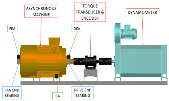
Figure 1.
Test bench.
It is worth noting that the bearings used at the transmission end were SKF 6205-2RS JEM (AB SKF, Gothenburg, Sweden), in which bores of 0.007, 0.014 and 0.021 inches were made. In addition, at the fan end, SKF 6203-2RS JEM were used, in which bores of 0.028 and 0.040 inches were made. Thus, the characteristics are listed in Table 1.

Table 1.
Bearing construction features.
Vibration data were collected using accelerometers, which were fixed to the housing with magnetic bases located above the shaft at both the drive end and the fan end of the motor housing. Vibration signals were collected using a 16-channel DAT recorder and further processed. In terms of sampling rate, digital data were obtained at both 12,000 and 48,000 samples per second. Speed and power data were collected using the torque transducer and recorded by hand.
Rolling bearings consist of several different components: inner ring, balls or rollers, cage and outer ring (Figure 2). Damage to any of these elements causes one or more characteristic frequencies to appear in the frequency spectrum, allowing to identify them.
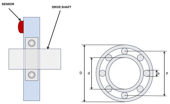
Figure 2.
Construction parameters of the bearing: D is the bearing outer diameter, d is the bearing inner diameter, b is the diameter of each ball, P is the pitch diameter.
The four possible frequencies of wear characteristic of a bearing and their mathematical expressions are as follows:
- -
- Ball pass frequency of the outer race or BPFO: The frequency with which defects in the outer ring pass through the rolling elements. Physically, this is the number of balls or rollers that pass a point on the outer race each time the shaft rotates one complete revolution. If there is a crack or a pitting defect in the outer race, every time a rolling element moves over it, a small impact occurs, generating vibrations at this frequency. When performing vibration analysis, an increase in amplitude at this frequency suggests an outer race fault.
- -
- Ball pass frequency of the inner race or BPFI: The frequency with which rolling elements cross defects in the inner ring. Physically, this is the number of balls or rollers that pass a point on the inner race each time the shaft completes a full revolution. A defect on the inner race produces periodic impacts as each rolling element moves over it, generating vibrations at this frequency. Unlike outer race defects, inner race defects usually change frequency with load or speed variations because the inner ring rotates with the shaft.
- -
- Ball spin frequency or BSF is the failure frequency of the rollers. Physically, this is the number of revolutions a bearing ball makes each time the shaft completes one full revolution. If a rolling element itself has a defect (such as a dent or crack), it will generate vibrations at this frequency as it rolls and contacts the races. However, BSF defects are harder to detect because rolling elements do not always make continuous contact with the raceways.
- -
- Fundamental cage frequency or FTF (Fundamental train frequency) is the rotation frequency of the cage containing the rolling elements. Physically, this is the number of revolutions that the bearing cage makes each time the shaft makes one complete revolution. A cage defect (such as misalignment or wear) disrupts the normal rolling motion of the bearing and can cause uneven loading, leading to vibrations at this frequency. However, cage defects are less common than raceway or rolling element defects.
According to the notation used in the equations, Nb corresponds to the number of balls, b to the diameter of each ball, P to the pitch diameter, the angle β to the contact angle of the balls with the outer and inner races, and rpm is the rotational frequency of the shaft.
2.2. Fault Diagnosis Methodology
The methodology used in this study for fault detection in rotating electrical machine bearings follows a structured approach. It begins with data acquisition, where vibration signals are collected from the Case Western Reserve University (CWRU) database using sensors. These signals are stored in an appropriate format for further analysis. Next, data preprocessing is performed to enhance signal quality. This involves filtering and removing noise, normalizing and segmenting the signals. Once the signals are preprocessed, they are transformed into scalograms, which are two-dimensional representations of time–frequency characteristics. This step employs wavelet transforms, specifically the amor and morse wavelets, to highlight fault patterns. The resulting scalogram images are stored for neural network training. In the training phase, a deep learning approach is applied using transfer learning with the SqueezeNet convolutional neural network. The model is fine-tuned by configuring hyperparameters such as the learning rate, number of epochs and minibatch size. The network is trained on the scalograms and validated using test data to ensure reliability. After training, the model is evaluated and optimized. Performance is assessed using a confusion matrix, which helps identify misclassifications. Hyperparameters are adjusted as needed, and comparisons between different wavelet transforms are made to determine the most effective feature extraction method. Finally, the trained model is deployed for fault classification and diagnosis. It is used to analyze new vibration data and classify conditions as either normal, inner race fault or outer race fault. Based on the predictions, reports are generated, and alerts are issued for predictive maintenance, helping to prevent costly machine failures and downtime. (Figure 3).
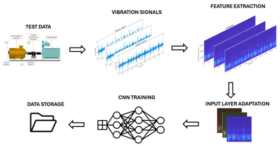
Figure 3.
Outline of the methodology.
In this study, SqueezeNet was selected for transfer learning due to its efficiency in extracting meaningful features from scalograms while maintaining a compact architecture. However, other lightweight convolutional neural networks, such as MobileNet and ShuffleNet, are also commonly used in similar applications. A comparative analysis of these architectures provides deeper insight into the advantages of choosing SqueezeNet over alternative models. MobileNet employs depthwise separable convolutions, significantly reducing computational cost while maintaining high classification accuracy. It is particularly effective in mobile and embedded systems where computational resources are limited. Similarly, ShuffleNet optimizes efficiency by introducing pointwise group convolutions and channel shuffling, which enhance computational speed and reduce model complexity. These architectures have been widely adopted in tasks that require real-time inference with limited hardware capabilities. SqueezeNet, on the other hand, was designed specifically to achieve a significantly smaller model size. By utilizing fire module combinations of squeeze and expand layers, it dramatically reduces the number of parameters while maintaining high accuracy. This architecture is particularly well suited for fault diagnosis applications, where real-time processing and low memory usage are essential. Additionally, the reduced model size of SqueezeNet enables faster inference speeds, making it an optimal choice for industrial settings where rapid fault detection is critical. A preliminary assessment suggests that while MobileNet and ShuffleNet offer competitive accuracy, SqueezeNet achieves similar classification performance with fewer parameters, leading to reduced memory consumption and faster training times. This balance between efficiency and accuracy reinforces its suitability for the proposed fault diagnosis system.
The methodology also includes continuous optimization, where machine learning algorithms are fine-tuned and improved as feedback is obtained on their performance. This iterative approach seeks to maximize accuracy and minimize false positives and negatives in fault diagnosis. The process is explained in the following sections.
2.2.1. Vibration Signal Processing
An illustrative example of the vibration signals in the time domain is presented below in Figure 4, specifically for a 0.007” diameter flaw.
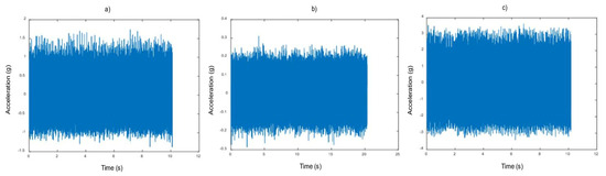
Figure 4.
Representation of the original vibration signals: (a) Inner track failure; (b) No failure; (c) Outer track failure.
A more detailed analysis of these signals, in addition to observing the presence of noise in them, shows that the signals affected by the fault have a duration of 10 s, in contrast to the signals of bearings without fault, which have a duration of 20 s. For this reason, a normalization process is carried out, and the signals are segmented into 0.1 s intervals. In this way, 200 segments are obtained from the signals with a duration of 20 s, while 100 segments are generated from those with a duration of 10 s, thus allowing a homogenization in the analysis, as can be seen in Figure 5.
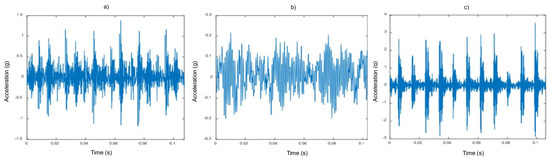
Figure 5.
Representation of the standardized vibration signals: (a) Inner track failure; (b) No failure; (c) Outer track failure.
Given the limited availability of ball bearing failure data in the database, it has been decided to avoid their inclusion in the study. This choice is based on the search for greater effectiveness in the training of the neural network, allowing it to concentrate on the classification of failures already identified and documented with sufficient representation in the available data. By reducing the complexity of the problem by focusing on specific failures with sufficient data, the aim is to improve the accuracy and robustness of the classification model, thus more effectively fulfilling the main objective of this research work, which is the correct identification and classification of the existing failure signals in the conditions of this database.
2.2.2. Time Frequency Analysis
Vibration signals obtained from failed bearings have characteristics that can be obtained by spectrum analysis. Therefore, we begin by representing the vibration signals from the bearings in the Matlab environment together with their respective scalograms. This is done to visualize the relationship between the signal in the time domain and its representation in the time–frequency domain by means of the scalogram. It is important to remember that a scalogram is a two-dimensional representation of a signal that shows how its energy varies over time and in different frequency bands. Therefore, each point in the scalogram corresponds to a specific moment in time and to a particular frequency. This allows to observe how the characteristics of the signal, the vibration peaks or oscillations, manifest themselves at different frequencies as it evolves over time.
This representation is particularly useful since bearing failures generate specific vibration patterns over time and at different frequencies. For example, a failure on the outer race might manifest as a series of high-energy spikes at certain frequencies, while a failure on the inner race might have a different pattern.
Figure 6 shows the vibration signal from a normal bearing without failure. Despite not having any defects, the signal in Figure 6 has a certain amplitude of vibration that is completely normal and corresponds to its base spectrum. In addition, the scalogram shows a more uniform energy, contrary to what was observed in previous cases.
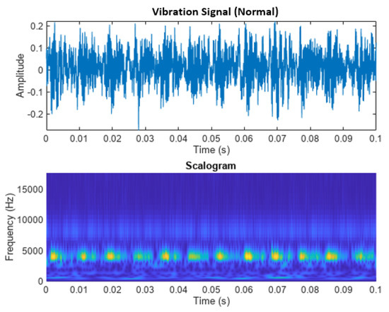
Figure 6.
Sign and scalogram of a healthy bearing.
Figure 7 shows the vibration signal from a bearing with a failure on the outer race. During the 0.1 s shown in Figure 7, the vibration signal contains 16 pulses because the BPFI of the bearing is 159.63 Hz. If we divide this number of pulses by the 0.1 s of representation the result is 160 Hz. Consequently, the scalogram shows the alignment of the 16 peaks with the pulses of the vibration signal.
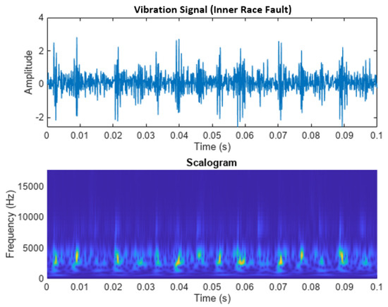
Figure 7.
Signal and scalogram of a fault in the inner race of a bearing.
Figure 8 shows the vibration signal of a fault in the outer track with its scalogram. In this case, although barely noticeable to the naked eye, the outer race failure shows 7 distinct peaks during the first 0.1 s, which is consistent with the ball passing frequencies of 75.06 Hz. Because the pulses in the time domain signal are not as prominent as in the inner race failure case, the distinct peaks in the scalogram show less contrast with the background.
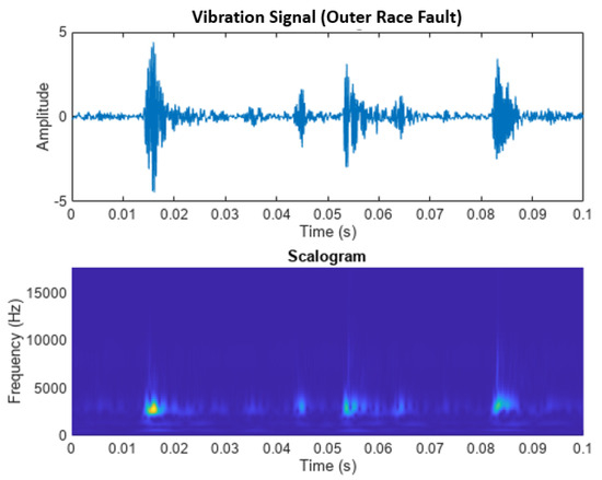
Figure 8.
Signal and scalogram of a fault in the outer race of a bearing.
The number of distinct peaks is a good characteristic to differentiate between inner race failures, outer race failures and normal conditions. Therefore, a scalogram can be a good candidate for classifying bearing failures.
Subsequently, to automate this process of transforming signals into scalograms, a helper function has been created in Matlab. This function allows to input a vibration signal and obtain its scalogram quickly and efficiently. This facilitates the analysis of a large volume of vibration signal data and helps to identify fault patterns in a more systematic way.
2.2.3. Input Layer Adaptation
Knowing how the data have been structured, the next step is to configure a data warehouse. For this purpose, Matlab specifically has the “fileEnsembleDatastore” function, which specializes in the development of algorithms used in predictive maintenance. When using this data store, it is necessary to specify the path where the files are located, their extension, as well as define the data variables that will be available in the store (“DataVariables”), the variables that describe the conditions or labels of the data (“ConditionVariables”) and the property that lists all the variables that will be available in the data store (“SelectedVariables”).
Similarly, a custom function is used by calling the “ReadFcn” function in the code and assigning it the arbitrary name “@readCWRUBearing”. This will facilitate the task of reading and processing the data, simplifying and optimizing the code.
Next, the one-dimensional vibration signals are converted into scalograms, and the images are archived for use in the training process. Each scalogram is sized to 227 by 227 by 3, which matches the input format required by the SqueezeNet neural network. To improve the programming code, a helper function called “convertSignalToScalogram” has been designed that takes the signal in its raw state and splits it into multiple segments. After the program is executed, a folder called “train_image” is automatically generated in the directory where Matlab is working. All scalogram images corresponding to the bearing signals in the folder called “train_data” will be stored in the folder “train_image”.
To avoid overtraining, the data have been segmented into training and validation sets. For this purpose, using the Matlab function “splitEachLabel”, 80% of the images located in the “train_image” folder are used for the training phase, and the remaining 20% are used for the validation set.
2.2.4. Transfer Learning Training
Following the order established in the methodology, we proceed to adapt the previously trained convolutional neural network “SqueezeNet” to carry out the task of classifying scalograms. It is important to note that “SqueezeNet” has previously been subjected to rigorous training with a dataset of more than one million images, which has allowed it to acquire highly enriched feature representations. In the transfer learning technique, a pre-trained network is taken and used as a starting point for a new task. This approach is considerably more efficient in terms of time and resources compared to training a network from scratch with randomly initialized weights. In addition, it enables the rapid transfer of learned features, even with a smaller training dataset.
Specifically, in “SqueezeNet”, the convolutional layer called “conv10” is used for the extraction of key features of the image and the classification layer identified as “ClassificationLayer_predictions” to carry out the classification of the input image. Both layers are essential in the process of combining the features extracted by the network into probabilities associated with each class, thus determining the loss value and the prediction labels. When “SqueezeNet” needs to be retrained to classify new images, it is necessary to replace the layers with new layers that are specifically adapted to the characteristics of the images of interest.
In most neural network architectures, the last layer that can be fine-tuned during training is usually a layer known as the “fully connected” or “fullyConnectedLayer”. However, in networks like SqueezeNet, this last layer is 1 by 1 in size. In this work, this convolutional layer is replaced with a new one that has several filters equal to the number of classes we want to classify. Additionally, the classification layer that assigns the network’s output classes is replaced by a new layer that does not include class labels. By using the “trainNetwork” function, it automatically adjusts the output classes during the training process.
To control the learning rate in the transferred layers, we made use of the “trainingOptions” function in Matlab and set a relatively low initial learning rate. Then, after having created the new convolutional layer, we increased the learning rates in the new final layers. This combination of learning rate settings results in fast learning exclusively in the newly added layers, while the other layers learn more gradually. Moreover, during the transfer learning process, it is not necessary to perform many training epochs. It is worth mentioning that one epoch is equivalent to a complete training cycle covering the entire dataset. On the other hand, the “ValidationFrequency” option in the “trainingOptions” function allows validating the network at each iteration during training by setting a specific value.
The following parameters have been used in the network training options consistently, to evaluate the influence of the wavelet transform and the learning rate:
- -
- MaxEpochs = 4 (maximum number of training epochs)
- -
- Shuffle = every-epoch (change the order of training and validation data before each training epoch)
- -
- Validation frequency = 30 (validation frequency in number of iterations)
- -
- MiniBatchSize = 20 (minibatch size for each training iteration)
2.2.5. Training Data Validation
To verify the accuracy of the trained neural network model, it is necessary to apply the same processing to the test data as was used on the training data. In this case, the test data are in the “test_data” folder.
Once this process is complete, we proceeded to classify the test image dataset using the pre-trained network. From this point, the accuracy of the predictions made by the model can be evaluated and represent the confusion matrix, which gives detailed information about the effectiveness of the model in classifying the test samples.
Multiple trainings of the network are carried out, verifying that there is some variability in the precision of the predictions between iterations. However, the average accuracy remains around 99%. Although the training dataset is relatively small in size, this example demonstrates that transfer learning is beneficial and manages to achieve a considerably high level of accuracy.
3. Results
In the task of optimizing fault diagnosis in rotating machine bearings by applying deep learning technology, various experiments have been carried out in the training process in which two types of wavelets have been used: the “amor” (analytical morlet Gabor wavelet) and the “morse” (generalized morse wavelet). The distinction between “amor” and “morse” wavelets primarily lies in their mathematical formulation and flexibility, which impacts their application to data analysis. The amor (analytic Morlet) wavelet is a commonly used wavelet in continuous wavelet transforms (CWTs) due to its close resemblance to the Fourier transform, making it well suited for time–frequency analysis of signals with well-defined oscillatory components. However, it lacks full adaptability in terms of shape parameters. The morse wavelet, on the other hand, provides greater flexibility because it is defined by two parameters (symmetry and time-decay), allowing it to adapt better to different signal characteristics. This adaptability makes morse wavelets more useful in analyzing a broader range of signals, especially in cases where the amor wavelet may not be optimal. In terms of practical application, the amor wavelet is often preferred for general-purpose time–frequency analysis due to its simplicity and frequency localization properties. The morse wavelet can be tuned to different types of signals, potentially leading to better resolution and interpretability in certain cases, such as non-stationary or highly transient signals.
Likewise, these parameters have been studied independently, and with the same values, in correlation with the learning rate to find out how the neural network behaves. In this sense, it started with an initially high learning rate and has been reduced exponentially. These tests have been carried out to examine the impact of the wavelets and the variation in the learning rate on the performance of this transfer learning neural network model.
Firstly, the results obtained in the training and validation process regarding the amor wavelet in the neural network have been compiled in Table 2.
Table 2.
Results with the training data with the application of the amor wavelet.
If the wavelet transform is replaced by morse and configured with the same learning rate values, the results of the training and validation of the neural network are shown in Table 3.
Table 3.
Results with training data using the morse wavelet application.
Next, the results obtained during the testing process in the neural network are analyzed, in which both wavelet transforms have been used in correlation with the confusion matrix. It is also worth mentioning that the following tables indicate, on the one hand, the values correctly predicted by the network for the three identified classes (inner race fault, normal and outer race fault) and, on the other hand, the values of the incorrectly predicted classes (misclassified). Thus, with respect to those obtained with the amor wavelet, the results of the confusion matrices for different learning rates can be verified in Table 4.
Table 4.
Results with test data using the amor wavelet application.
Replacing the amor wavelet transform with the morse wavelet and applying the same learning rate values again, the results in the test phase are presented in Table 5.
Table 5.
Results with test data using the morse wavelet application.
4. Discussion
To discuss in detail the above results regarding accuracy and training time, Figure 9 and Figure 10 have been developed. In these Figures accuracy an training time are compared for cases A to E, where the learning rate is progressively reduced.
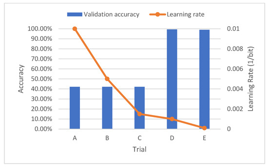
Figure 9.
Accuracy with training data and amor wavelet.
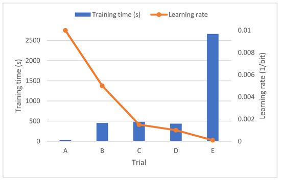
Figure 10.
Training time and amor wavelet.
Regarding the first graph, the accuracy starts at a low level, specifically below 50%, when starting with a learning rate of 0.01. As the learning rate is reduced, accuracy increases, although not significantly. However, to achieve satisfactory results, it is necessary to decrease the learning rate considerably, specifically below 0.0015, as observed in test C. Regarding the training time, the behavior is like the learning rate, that is, it increases exponentially as the learning rate is reduced.
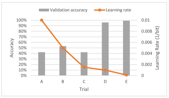
Figure 11.
Accuracy with training data using the morse wavelet.
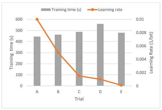
Figure 12.
Time with training data using the morse wavelet.
According to the results, if high values are applied to the learning rate, low accuracy is obtained. On the other hand, if they are reduced enough, high accuracy is obtained, in the same way as with the results of the previous wavelet. However, it can be observed that the trend is not the same as in the previous case.
On the other hand, regarding the training time, it is observed that it is relatively short and that, in addition, it remains constant, even with low learning rates. This aspect is also interesting if we compare it with the training time results of the previous wavelet.
Likewise, to more conveniently assess the precision, the results have been represented in Figure 13 and Figure 14.
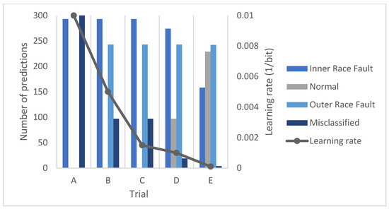
Figure 13.
Accuracy results with test data using the amor wavelet.
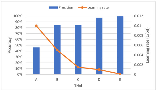
Figure 14.
Average accuracy results with test data using the amor wavelet.
As can be seen, the above results are quite clear, since as the learning rate decreases, the number of classes correctly predicted by the network increases. In fact, this can also be seen reflected in the accuracy graph.
On the other hand, if the number of predictions is considered, the network identifies a greater number of faults located in the inner track. In this regard, it should be noted that as the learning rate decreases, the number of predictions for each class tends to equalize.
Again, to more conveniently assess the accuracy, the same graphs have been represented for the morse wavelet results, as seen in Figure 15 and Figure 16.
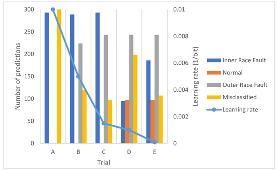
Figure 15.
Accuracy results with test data using the morse wavelet.
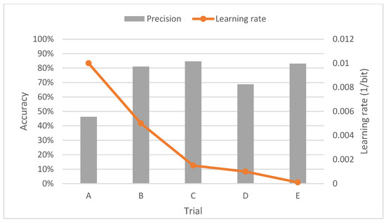
Figure 16.
Average accuracy results with test data with the application of the morse wavelet.
As with the other wavelet transform, the results are enlightening, since as the learning rate is reduced, the number of classes correctly predicted by the network increases. However, the overall accuracy remains relatively constant, although with a slight increase as the learning rate is reduced.
In regard to the number of predictions, once again, the network detects a higher number of errors in the internal track. In addition, there is a tendency to equalize the number of correct predictions as we decrease the learning rate. On the other hand, the maximum results obtained from the tests and their general representation can also be exposed, both in the training and validation phase and in the test phase (Figure 17).
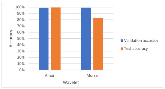
Figure 17.
Maximum precision results.
It should be noted that, to conclude which of the results is better in terms of accuracy, that is, which has the highest precision, it is necessary to observe the results obtained only with the data from the test group, since these are the ones that the neural network evaluates after having been trained. On this premise, it can be stated that the best result is obtained using the amor wavelet with an accuracy of 99.34% at a learning rate of 0.0001.
To highlight how our results compare with prior studies, [7] presents a review of bearing fault detection and diagnosis using the Case Western Reserve University dataset with deep learning approaches. Models like convolutional neural networks (CNNs) achieved up to 99.91% accuracy without requiring preprocessing, while Deep Belief Networks (DBNs) reached 100% accuracy, even in noisy environments. Additionally, Generative Adversarial Networks (GANs) have enhanced fault detection by generating synthetic data. On the other hand, strategies like Reinforcement Learning (RL) have shown improvements in detection without the need for labeled data, and transfer learning with ResNet-50 achieved an accuracy of 99.99%, outperforming models such as VGG-16 and VGG-19.
Results in our study indicate that precise hyperparameter tuning enhances diagnostic accuracy. Scalograms proved particularly effective in identifying distinct vibration patterns for faults in bearings’ inner and outer races. Scalograms have been employed in this study to convert one-dimensional time-domain signals into two-dimensional time–frequency representations. Scalograms provide a highly localized time–frequency representation, making them particularly useful for analyzing transient and non-stationary signals, such as vibration signals from faulty bearings. Unlike the Short-Time Fourier Transform (STFT), which uses a fixed window size and may lead to poor time–frequency resolution trade-offs, the wavelet transform adapts its resolution dynamically. High-frequency components are represented with fine time resolution, while low-frequency components maintain high frequency resolution. This adaptability is critical in bearing fault diagnosis, where faults often generate impulses that appear as transient events within the signal. Compared to the Hilbert–Huang Transform (HHT), which decomposes signals into intrinsic mode functions (IMFs) using empirical mode decomposition (EMD), wavelet-based scalograms offer a more robust representation without requiring additional signal decomposition steps. While HHT is effective for extracting mode-dependent features, it is highly sensitive to noise and mode-mixing issues, which may introduce artifacts in the time–frequency representation. Additionally, the MUSIC algorithm, which is based on eigenvalue decomposition for spectral estimation, is effective for resolving closely spaced frequency components but lacks the ability to capture time-domain variations effectively. Since bearing faults manifest as transient events rather than stationary frequency components, MUSIC is less suited for this application.
5. Conclusions
The results of applying the proposed methodology for predicting bearing failures offer valuable insights into the field of predictive maintenance. Through rigorous analysis and experimentation, the capabilities and limitations of this approach in early detection of bearing problems have been identified, highlighting its potential as an effective tool for improving the reliability and efficiency of rotating machines in industrial environments.
The results of this study reveal the evolution in accuracy throughout the training process of the neural network. This means that as the network gains more knowledge through training, its ability to make accurate predictions improves significantly. It is also evident that the proper tuning of the hyperparameters, such as the learning rate, plays an essential role in this process. When properly configured, these hyperparameters allow for promising results in detecting bearing faults with high accuracy, which is essential in predictive maintenance and machinery diagnostic applications.
The correct selection of hyperparameters is a key consideration in the development of machine learning models. This study demonstrates that by carefully choosing these values, the variability in the results obtained can be significantly reduced. Consequently, greater consistency in the convergence of the results is observed, which facilitates the interpretation and practical application of the neural network in the detection of bearing faults and other industrial applications. A broader exploration of hyperparameters could further optimize model performance. Although initial tuning was performed, it would be interesting to expand hyperparameter search range using cross-validation techniques in future studies.
Regarding the feasibility of using transfer learning, the results obtained in this study are fruitful in applying this technique in a new case study. Transfer learning proves to be a valuable tool that improves not only the generalization capability of the model, but also its convergence speed and accuracy. This is particularly noteworthy given that these outstanding results are achieved with a relatively small dataset compared to more conventional applications such as object recognition. In summary, transfer learning shows significant potential for industrial and diagnostic applications, supporting its utility and feasibility in improving predictive maintenance and machinery diagnostic systems. It has been acknowledged the importance of testing on actual industrial sites. While this study was based on the CWRU dataset, future work will focus on real-world validation under complex operating conditions to assess noise robustness and environmental adaptability.
Future research should explore the potential of hybrid models that combine deep learning with classical machine learning techniques, like Support Vector Machines or Random Forest, to enhance the robustness of fault detection systems. Another key area of study is the interpretability of deep learning models, as developing methods to explain neural network decisions would improve trust and facilitate adoption in industrial environments. Additionally, integrating multi-sensor data, such as temperature and acoustic emissions, could create a more comprehensive diagnostic system. Real-time adaptation through online learning techniques would allow the model to continuously update with new data, further improving its predictive capabilities. Finally, cross-dataset validation on different bearing fault datasets beyond the CWRU database would help assess the generalization of the proposed method across various machines and industrial settings.
In industrial applications, deploying this methodology on edge computing platforms could enable real-time fault monitoring, reducing unplanned downtime and maintenance costs. Integrating the approach into predictive maintenance systems would automate fault detection in large-scale industrial operations, improving reliability and efficiency. Optimization for low-power embedded systems would also allow implementation in resource-limited environments, making fault diagnosis more accessible in remote industrial settings.
Author Contributions
Conceptualization, E.Q.-C.; methodology, A.G.-B. and E.Q.-C.; software, A.G.-B. and I.A.-M.; validation, A.G.-B. and I.A.-M.; formal analysis, A.G.-B., G.E.-E. and I.A.-M.; investigation, A.G.-B., E.Q.-C. and G.E.-E.; resources, E.Q.-C. and G.E.-E.; data curation, A.G.-B. and I.A.-M.; writing—original draft preparation, E.Q.-C. and A.G.-B.; writing—review and editing, E.Q.-C. and I.A.-M.; visualization, E.Q.-C. and G.E.-E.; supervision, E.Q.-C. and G.E.-E.; project administration, E.Q.-C.; funding acquisition, E.Q.-C. and G.E.-E. All authors have read and agreed to the published version of the manuscript.
Funding
Funding support has been received from the research support plan of the Instituto de Automática e Informática Industrial ai2, Universitat Politècnica de València.
Institutional Review Board Statement
Not applicable.
Informed Consent Statement
Not applicable.
Data Availability Statement
The original contributions presented in the study are included in the article, further inquiries can be directed to the corresponding author.
Conflicts of Interest
The authors declare no conflicts of interest.
References
- García, E.; Quiles, E.; Correcher, A.; Morant, F. Predictive Diagnosis Based on Predictor Symptoms for Isolated Photovoltaic Systems Using MPPT Charge Regulators. Sensors 2022, 22, 7819. [Google Scholar] [CrossRef] [PubMed]
- García, E.; Quiles, E.; Zotovic-stanisic, R.; Gutiérrez, S.C. Predictive Fault Diagnosis for Ship Photovoltaic Modules Systems Applications. Sensors 2022, 22, 2175. [Google Scholar] [CrossRef] [PubMed]
- Ochoa, J.; García, E.; Quiles, E.; Correcher, A. Redundant Fault Diagnosis for Photovoltaic Systems Based on an IRT Low-Cost Sensor. Sensors 2023, 23, 1314. [Google Scholar] [CrossRef] [PubMed]
- Muthukumaran, S.; Rammohan, A.; Sekar, S.; Maiti, M.; Bingi, K. Bearing Fault Detection in Induction Motors Using Line Currents. ECTI Trans. Electr. Eng. Electron. Commun. 2021, 19, 209–219. [Google Scholar] [CrossRef]
- Cascales-Fulgencio, D.; Quiles-Cucarella, E.; García-Moreno, E. Computation and Statistical Analysis of Bearings’ Time- and Frequency-Domain Features Enhanced Using Cepstrum Pre-Whitening: A ML- and DL-Based Classification. Appl. Sci. 2022, 12, 10882. [Google Scholar] [CrossRef]
- Rolling Element Bearing Fault Diagnosis. Available online: https://es.mathworks.com/help/predmaint/ug/Rolling-Element-Bearing-Fault-Diagnosis.html (accessed on 12 December 2024).
- Neupane, D.; Seok, J. Bearing Fault Detection and Diagnosis Using Case Western Reserve University Dataset with Deep Learning Approaches: A Review. IEEE Access 2020, 8, 93155–93178. [Google Scholar] [CrossRef]
- Pacheco-Chérrez, J.; Fortoul-Díaz, J.A.; Cortés-Santacruz, F.; María Aloso-Valerdi, L.; Ibarra-Zarate, D.I. Bearing Fault Detection with Vibration and Acoustic Signals: Comparison among Different Machine Leaning Classification Methods. Eng. Fail. Anal. 2022, 139, 106515. [Google Scholar] [CrossRef]
- Kiral, Z.; Karagülle, H. Vibration Analysis of Rolling Element Bearings with Various Defects under the Action of an Unbalanced Force. Mech. Syst. Signal Process 2006, 20, 1967–1991. [Google Scholar] [CrossRef]
- Sawalhi, N.; Randall, R.B. Vibration Response of Spalled Rolling Element Bearings: Observations, Simulations and Signal Processing Techniques to Track the Spall Size. Mech. Syst. Signal Process. 2011, 25, 846–870. [Google Scholar] [CrossRef]
- Smith, W.A.; Randall, R.B. Rolling Element Bearing Diagnostics Using the Case Western Reserve University Data: A Benchmark Study. Mech. Syst. Signal Process. 2015, 64–65, 100–131. [Google Scholar] [CrossRef]
- Heidari, A.; Navimipour, N.J.; Unal, M. Applications of ML/DL in the Management of Smart Cities and Societies Based on New Trends in Information Technologies: A Systematic Literature Review. Sustain. Cities Soc. 2022, 85, 104089. [Google Scholar] [CrossRef]
- Dong, S.; Yin, S.; Tang, B.; Chen, L.; Luo, T. Bearing Degradation Process Prediction Based on the Support Vector Machine and Markov Model. Shock Vib. 2014, 2014, 717465. [Google Scholar] [CrossRef]
- Pandya, D.H.; Upadhyay, S.H.; Harsha, S.P. Fault Diagnosis of Rolling Element Bearing with Intrinsic Mode Function of Acoustic Emission Data Using APF-KNN. Expert. Syst. Appl. 2013, 40, 4137–4145. [Google Scholar] [CrossRef]
- Piltan, F.; Prosvirin, A.E.; Jeong, I.; Im, K.; Kim, J.M. Rolling-Element Bearing Fault Diagnosis Using Advanced Machine Learning-Based Observer. Appl. Sci. 2019, 9, 5404. [Google Scholar] [CrossRef]
- Pan, J.; Zi, Y.; Chen, J.; Zhou, Z.; Wang, B. LiftingNet: A Novel Deep Learning Network with Layerwise Feature Learning from Noisy Mechanical Data for Fault Classification. IEEE Trans. Ind. Electron. 2018, 65, 4973–4982. [Google Scholar] [CrossRef]
- Zhao, Z.; Li, T.; Wu, J.; Sun, C.; Wang, S.; Yan, R.; Chen, X. Deep Learning Algorithms for Rotating Machinery Intelligent Diagnosis: An Open Source Benchmark Study. ISA Trans. 2020, 107, 224–255. [Google Scholar] [CrossRef]
- Duong, B.P.; Kim, J.Y.; Jeong, I.; Im, K.; Kim, C.H.; Kim, J.M. A Deep-Learning-Based Bearing Fault Diagnosis Using Defect Signature Wavelet Image Visualization. Appl. Sci. 2020, 10, 8800. [Google Scholar] [CrossRef]
- Escrivá-Escrivá, G.; Álvarez-Bel, C.; Roldán-Blay, C.; Alcázar-Ortega, M. New Artificial Neural Network Prediction Method for Electrical Consumption Forecasting Based on Building End-Uses. Energy Build. 2011, 43, 3112–3119. [Google Scholar] [CrossRef]
- Liu, X.; Ma, H.; Liu, Y. A Novel Transfer Learning Method Based on Conditional Variational Generative Adversarial Networks for Fault Diagnosis of Wind Turbine Gearboxes under Variable Working Conditions. Sustainability 2022, 14, 5441. [Google Scholar] [CrossRef]
- Jose Saucedo-Dorantes, J.; Arellano-Espitia, F.; Delgado-Prieto, M.; Alfredo Osornio-Rios, R.; Glowacz, A.; Antonino-Daviu, J.A.; Caesarendra, W. Diagnosis Methodology Based on Deep Feature Learning for Fault Identification in Metallic, Hybrid and Ceramic Bearings. Sensors 2021, 21, 5832. [Google Scholar] [CrossRef]
- Liu, Z.; Tan, C.; Liu, Y.; Li, H.; Cui, B.; Zhang, X. A Study of a Domain-Adaptive LSTM-DNN-Based Method for Remaining Useful Life Prediction of Planetary Gearbox. Processes 2023, 11, 2002. [Google Scholar] [CrossRef]
- Welcome to the Case Western Reserve University Bearing Data Center Website|Case School of Engineering. Available online: https://engineering.case.edu/bearingdatacenter/welcome (accessed on 9 December 2024).
Disclaimer/Publisher’s Note: The statements, opinions and data contained in all publications are solely those of the individual author(s) and contributor(s) and not of MDPI and/or the editor(s). MDPI and/or the editor(s) disclaim responsibility for any injury to people or property resulting from any ideas, methods, instructions or products referred to in the content. |
© 2025 by the authors. Licensee MDPI, Basel, Switzerland. This article is an open access article distributed under the terms and conditions of the Creative Commons Attribution (CC BY) license (https://creativecommons.org/licenses/by/4.0/).