Modeling and Simulation of Standing Wave Configurations for Outflow Improvement and Minimizing Undesired Recirculation

Abstract

River surfing has evolved from natural rivers to artificial standing waves, like the Fuchslochwelle in Nuremberg, where optimizing wave quality and safety remains a challenge. Key issues include recirculation zones that pose risks, particularly at higher inflows. This study addresses safety and performance improvements by introducing geometric modifications to reduce recirculation zones. Using STAR-CCM+ simulations, 16 configurations of baffles and inlays were analyzed. A 3D-CAD model of the Fuchslochwelle was developed to test symmetrical and asymmetrical configurations, focusing on reducing vorticity. Results showed that baffles placed 2 m from the inlay reduced recirculation zones by over 50%. Asymmetrical setups, combining wall and inlay baffles, also proved effective. Following simulations, a baffle was installed at 3 m, enhancing safety and quality. Previously, inflows above 7.5 m³/s caused dangerous backflow, requiring surfers to swim or dive to escape turbulence. With the baffle, safe operation increased to 9 m³/s, a 20% improvement, making the system suitable for surfers of all skill levels. These finding provide a novel approach to enhancing flow dynamics, applicable to a wide range of artificial standing waves. The valuable insights gained enable operators to optimize the dynamics and accessibility through geometric modifications while ensuring safety for users.

1. Introduction

River surfing, characterized by standing waves remaining stationary over time, has grown in popularity since its inception in 1972 by the Pauli brothers in Munich, Germany. Initially, natural river features created these waves, but modifications to riverbeds and the development of artificial systems have allowed the sport to spread globally. Notable examples include the Eisbachwelle in Munich and waves in the Snake River in Wyoming, USA. The recent trend of creating artificial standing waves in existing rivers, e.g., as seen in Hanover and Nuremberg (Germany), aims to provide surfing opportunities without direct ocean access [1,2]. However, since building these artificial waves is still in its inception and each wave geometry is different, optimal inflow and outflow conditions have not been achieved yet. Laminar inflow conditions facilitate a glassy and desired wave surface. Outflow conditions behind the wave should exhibit a constant downstream flow carrying the surfer away from the wave. Recirculation areas (Figure 1) and back flow should be minimized or avoided since these may drag the surfer back into the wave, endangering them.

Reducing the water flow rate (m³/s) is one way to reduce such potential endangering characteristics; however, this leads to reduced wave quality. Hence, in this study, we focus on improving outflow conditions by changing the bottom topology behind the wave by simultaneously improving the wave quality, i.e., enabling more water flow. This study simulates the surfing conditions at the Fuchslochwelle in Nuremberg whereby the concept can be transferred to any other standing waves. Despite the growing popularity of river surfing, research in this area remains limited compared to studies on ocean waves. Early investigations by Hornung and Killen [4] focused on artificially generated waves to study the forces acting on surfboards. Subsequent research has expanded this notion to include numerical simulations [5,6,7] and experimental studies [8] on surfboard geometries and fin configurations [9,10]. Although numerical research on surfboard and fin dynamics is well documented, studies on surf waves themselves, particularly standing river waves, are sparse. Historical research on waves dates back hundreds of years, focusing primarily on ocean waves and artificial reefs designed for coastal protection and tourism enhancement. Scarfe et al. [11] provided an overview of surfing science, emphasizing the influence of coastal profiles on wave formation. Numerous studies [12,13,14,15] have explored the design and optimization of artificial reefs, combining experimental and numerical approaches to improve wave quality and shoreline protection. For standing river waves, the literature is less extensive. According to Fuchs [3], artificial river waves can be generated through various methods: sheet-flow on wave-like bathymetry (mapping of underwater topography), spatial wave tubes, hydraulic jumps at bottom drops, and hydraulic jumps with adjustable installations. The Fuchslochwelle utilizes the latter method, relying on hydraulic jumps—a phenomenon widely studied for energy dissipation and cavitation prevention [16,17,18,19,20,21]. Optimal river surf waves aim to create waves with a wide or long surfable face, allowing surfers to generate speed and maintain control, while minimizing air mixture (i.e., glassy surface). This is often achieved through abrupt channel bed drops but should avoid being overly steep to ensure better maneuverability for the surfer. Froude numbers between 2.5 and 3 typically result in surfable waves [20], though adjustable deflectors can produce waves at lower Froude numbers. Fuchs [3] also highlighted that the length of the recirculation zone behind the wave is critical for surfer safety, with shorter zones reducing the risk of injuries from tumbles. Oertel et al. [22] focused on small-scale surf waves to validate numerical solutions compared to experimental data, while Borman et al. [23] used a three-dimensional transient two-phase RANS CFD-VoF model to predict the position of waves and hydraulic jumps in a complex hydraulic environment, validated against full-scale experiments. They showed that two-phase CFD can predict hydraulic flow features in medium/large-scale open channel flows. Asiaban et al. [24] introduced a flat-bed technology for creating river surf waves without drops using a numerical model. Their study focused on wave sensitivity to ramp slope, tailwater depth, and kicker configurations. They found that the ramp slope has a minimal impact on the wave behavior, while kicker geometry and position, and tailwater depth can significantly reinforce and accelerate the wave. This study seeks to bridge the gap in the literature by presenting an adaptive and innovative approach to minimizing recirculation zones in artificial river surf waves, with a particular focus on configurations similar to the Fuchslochwelle. By conducting CFD simulations, this research aims to (1) gain insights into the flow field, (2) understand the factors contributing to recirculation zones, (3) propose geometric modifications that minimize these recirculation zones, and aim to (4) enhance surfer safety. This work involves 3D-CAD modeling of the Fuchslochwelle, a comprehensive high-performance-computation (HPC) simulation setup, and it also involves an analysis of different geometric configurations to identify the most effective design improvements regarding outflow conditions.

2. Materials and Methods

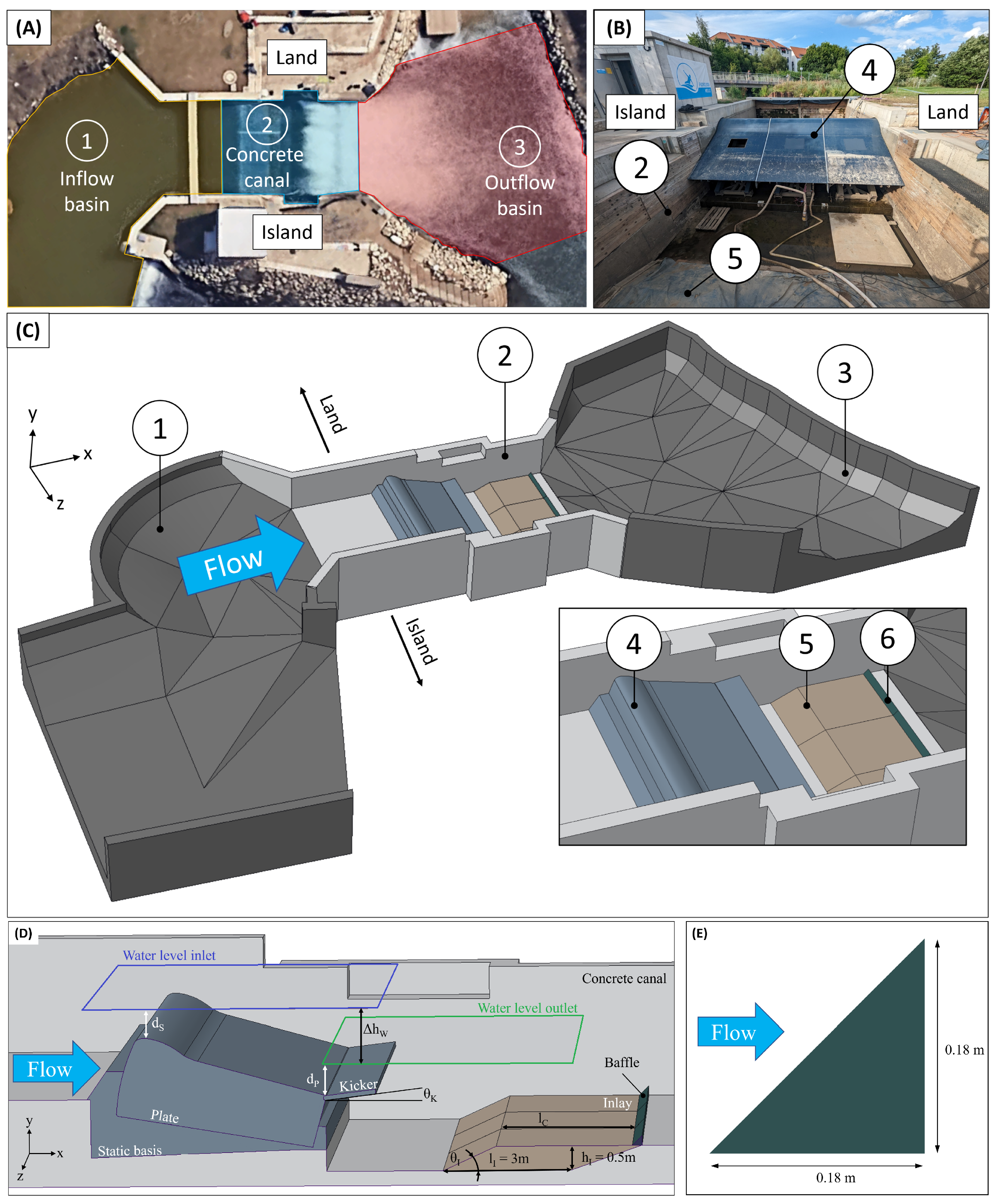
2.1. Geometry

The Fuchslochwelle comprises various components, as depicted in Figure 2. These include the inflow basin, a concrete canal where the wave module is installed, inlays, a baffle, and the outlet basin. The basins represent the natural riverbeds, which were measured prior to the study to ensure accurate representation, especially of the outflow topology. The wave module itself consists of several subcomponents, including a static base, a plate, and a so-called kicker, as illustrated in Figure 2D.

The CAD model was designed using PTC Creo Parametric v10.0 (PTC Inc., Boston, MA, USA). Each component was designed as a .prt file and assembled into a comprehensive .asm file. This approach allowed for the generation and simulation of various wave configurations. Figure 2D highlights the different parameters that can be changed to achieve different wave setups. Various parameters, including mass flow rate (Q), the difference between upper and lower water level ($\Delta h_W$), the distance between the plate and upper ($d_S$) and lower ($d_P$) water levels, the kicker angle (${\theta }_K$), and the inlay angle (${\theta }_I$), were kept constant throughout all conducted simulations, as shown in

Table 1. The constant parameters used in all simulations, including the mass flow rate (Q), the water level difference ($\Delta h_W$), the distances between the plate and the upper ($d_S$) and lower ($d_P$) water levels, and the kicker angle (${\theta }_K$) and the inlay angle (${\theta }_I$).

Environment		Wave Module			Inlay
Q/m3/s	$\Delta h_W$/m	$d_S$/m	$d_P$/m	${{\theta }_K/}^{\circ }$	$h_l$/m	$l_l$/m	${{\theta }_l/}^{\circ }$
9.3	1.14	0.717	0.91	6	0.5	3	24.65

.

This study focuses on installing and modifying baffles on the inlay, considering its asymmetries, angles, and position on the inlays. The geometry of the used baffle is shown in Figure 2E.

Table 2. The simulation names, along with the inlay and baffle setups are presented for the (A) symmetric configuration (SCB) and (B) asymmetric configuration with baffles at the bottom (ACB) and a symmetric configuration group with baffles on both the bottom and side walls (SCBW). Inlay setup defines which inlay is installed, with each entry referring to one inlay. For example, 0-1-0 means that only the inlay in the middle over the entire length of the concrete canal is placed. Similarly, the setup in the baffle column defines which baffle is installed, with each entry referring to one baffle. For example, 0-1-0 means that only the middle baffle is placed on the middle inlay. Symbols > and < denote baffles at the side walls, while \ and / denote diagonal baffles on the inlay. All geometric variants are shown in Figure 3.

(A)	Name	Inlay Setup	Baffle		Figure 3	(B)	Name	Inlay Setup	Baffle		Figure 3
			Setup	lc/m					Setup	lc/m
SCB	$S_D$	1-1-1	0-0-0	-	A1	ACB	$S_A$	1-1-1	1-1-1	3-2-3	C1
	$S_I$	0-1-0	0-0-0	-	A5		$S_{VF}$		\-1-/	\-2-/	C2
	$S_I^{1m}$	0-1-0	0-1-0	1	A6		$S_{VH}$		/-1-\	/-2-\	C3
	$S_I^{2m}$	0-1-0	0-1-0	2	A7	SCBW	$S_W$	1-1-1	>0-0-0<	-	B1
	$S_I^{3m}$	0-1-0	0-1-0	3	A8		$S_W^{1m}$		>1-1-1<	1	B2
	$S_C^{1m}$	1-1-1	1-1-1	1	A2		$S_W^{2m}$		>1-1-1<	2	B3
	$S_C^{2m}$	1-1-1	1-1-1	2	A3		$S_W^{3m}$		>1-1-1<	3	B4
	$S_C^{3m}$	1-1-1	1-1-1	3	A4

summarizes all the simulations conducted for the symmetric and asymmetric configurations of the inlay and baffle setups. A total of 15 wave/inlay/baffle simulations were performed to simulate the flow conditions. A final 16th simulation was performed using the actual implemented baffle geometry. A visual representation of the configurations is shown in Figure 3(A1–A8), which depicts the symmetric configuration with baffles at the bottom ($SCB$); Figure 3(B1–B4), which depicts the symmetric configuration with the baffles at the bottom and wall ($SCBW$); and Figure 3(C1–C3), which depicts the asymmetric configuration with baffles at the bottom ($ACB$).

2.2. Boundary Conditions and Setup

For the simulation, for the sake of computational effort and feasibility, we decided to exclude the inflow basin to decrease the simulation area. The inflow is defined as rectangular plane. Hence, the impact of the inflow basin on the wave characteristics and potentially on the recirculation zones has not been considered. Figure 4 illustrates the boundary conditions used in this study. For both the inlet and outlet boundaries (shown in red), a velocity inlet condition is applied.

By default, the direction of this condition is the inner normal direction. Specifically, for the outflow, the direction is adjusted to point outward (i.e., in the outer normal direction). This approach is based on the principle that the volume of water entering the domain is equal to the volume leaving it, maintaining constant water levels at both the inlet and outlet. The inlet water level is maintained at a constant height of 1.85 m, while the outlet water level is determined by the inlet level and the differential height $\Delta h_W$. The inflow and outflow velocities of the water are calculated based on the mass flow rate Q = 9.3 m³/s (see Table 1) of the simulation setup, divided by the cross-sectional area of the water inlet and outlet. For the air phase, the inflow and outflow velocities are set to 1 m/s to simulate the interaction with the atmospheric boundary conditions effectively. The air boundary (depicted in orange) was set to a pressure outlet condition of 0 Pa, related to the reference pressure of 101,325 Pa. For the wall boundaries (indicated in gray: bottom and side walls), a no-slip wall condition was employed. For the simulation, two distinct setups were employed. The first setup was utilized for simulating the initial 100 physical seconds, during which the system was in a transient state. To ensure numerical stability, a first-order time discretization with a time step of $\Delta t=0.01$ seconds and a sharpening factor of 0 was selected. For the next 100 physical seconds, a second-order time discretization with a $\Delta t=0.003$ seconds and a sharpening factor of 0.6 was used. Gravity was set to 9.81 m/s² in the negative y direction. The water was assumed to have a constant density of 997.5 kg/m³ and a constant dynamic viscosity of 8.89 × 10⁻⁴ Pa s. For air, the ideal gas law was applied. Additionally, the air was modeled with a constant dynamic viscosity of 1.855 Pa s.

2.3. Numerical Methods

To simulate the free boundary two-phase flow, the volume of fluid (VoF) method is used [25]. The flow is computed using the incompressible Navier–Stokes equations through a cell-centered finite volume method (FVM) with the CFD software STAR-CCM+ 2020.2 (Siemens PLM Software, Plano, TX, USA). The modeling of the turbulent flow is based on the Reynolds-Averaged Navier–Stokes (RANS) equations in combination with an SST (Menter’s Shear Stress Transport) $k-\omega$ turbulence model [26,27]. As previously described, two different time discretization setups are used. The first-order discretization is applied for the initial 100 physical seconds, followed by second-order time discretization for the subsequent 70 physical seconds, resulting in a total physical simulation time of 170 physical seconds. It is important to note that during the grid independence study, a total simulation time of 200 physical seconds was initially considered. However, it was observed that after 70 s of second-order time discretization, the results reached a sufficient level of convergence, with minimal changes occurring beyond this point considering the wave height and the average velocity magnitude at the probes. Therefore, for the final simulation, a total of 170 s was deemed adequate. The simulations were performed on the Meggie cluster at the RRZE of the University of Erlangen-Nuremberg. The 32 used nodes resulted in 64 Intel Xeon E5-2630v4 “Broadwell” chips (Intel Corp., Santa Clara, CA, USA) with 10 cores per chip.

2.4. Mesh Generation and Grid Independence Study

For the simulations, we employed a structured grid generation approach, utilizing the Trimmed Cell Mesher to create a hexahedral dominant mesh. This mesher is particularly adept at handling complex geometries (e.g., the ground and the interface between the two phases), ensuring that the mesh conforms well to the intricate details of the surf wave structure. The grid generation process involved several steps to refine the mesh and ensure accurate simulation results. Initially, a coarse grid was generated to outline the primary features of the simulation domain. Subsequent refinement steps were applied, particularly around critical regions such as the interface between the two phases of water and air. Boundary layer meshing techniques were employed to ensure that near-wall regions were adequately resolved, allowing for precise modeling of the boundary layer effects.

Table 3. Different prism layer setups employed to achieve $y+$ values > 30. Since velocity magnitudes vary across different locations in the simulation, various prism layer configurations are necessary to ensure the proper application of wall functions.

Setting	Name	Thickness	#Cells	Stretch Factor
1	Inflow	70 mm	8
2	Wave module	40 mm	12
3	Edge	60 mm	6	1.1
4	Refinement	50 mm	16
5	Global	50 mm	12

shows the different prism layer setups to achieve $y+$ values between 5 and 220. An exemplary mesh and corresponding $y+$ values can be found in the Supplementary Materials Section (Supplementary Figures S1 and S2).

Please note that we conducted the grid independence study using a simplified channel geometry. The difference lies in replacing the outlet basin with an extension of the concrete channel. This modification allows us to reduce computation time without neglecting the complex structures of the wave module. The decision to conduct the study with this simplified geometry is based on the assumption that the essential flow characteristics and turbulence structures relevant to grid independence are similar in both geometries. Therefore, the results of this study can be applied to the actual simulation volume, as the main flow features and grid resolution requirements determined in the simplified geometry are also applicable to the more complex geometry. The simplified geometry for the grid independence study can also be found in the Supplementary Materials Section (Supplementary Figure S3).

Table 4. Grids and runtimes used for the grid independence study. Setup 2 results in numerical instabilities on the coarsest grid. Results of the grid independence study: the average wave height over the last 1, 5, and 10 s, and the average velocities at different probe locations (see Figure 5) over the last second. For further simulations, Grid 3 is used as a compromise between accuracy and computation time. Also, the grid resolution is sufficient to resolve geometric features such as baffles.

Grid	#Nodes	Base Size	#Cells	Runtime/h Setup 1 per 100 s	Runtime/h Setup 2 per 100 s	Average Wave Height over the Last X Seconds/m			Average over the Last Second, of Velocity Magnitude at Probes/m/s
						1 s	2 s	3 s	Probe 1	Probe 2	Probe 3	Probe 4
1	32	2.3	$0.7\times {10}^6$	06:13	-	-	-	-	-	-	-	-
2	32	1.1	$1.1\times {10}^6$	06:20	16:50	0.96	0.94	0.95	2.88	5.03	5.29	5.42
3	32	0.6	$\mathbf{2.2}\times {\mathbf{10}}^{\mathbf{6}}$	10:16	19:46	0.92	0.92	0.93	2.68	5.00	5.28	5.35
4	32	0.5	$3.2\times {10}^6$	12:39	22:03	0.98	0.98	0.98	2.96	5.01	4.96	5.27
5	64	0.4	$5\times {10}^6$	16:38	28:24	0.90	0.90	0.92	2.96	5.02	4.98	5.37

shows tested grids and run times for the grid independence study. To validate the reliability of the simulation results, a comprehensive grid independence study was conducted. Multiple grids with varying levels of refinement were tested to ensure that the results were not unduly influenced by the grid size.

To determine the most suitable grid for this study, the velocity magnitude of the wave at four locations along the wave module and the wave height at a specific position are evaluated as criteria. Figure 5 illustrates the positions of the four probes (indicated by numbers 1–4) and the wave height measurement at Position 5. Table 4 presents the results for the average wave height over time periods of the last 1, 5, and 10 s, along with the average velocity magnitudes at the probe positions. Based on these evaluations, Grid 3 is selected for further simulations as it offers a balanced compromise between accuracy and computational efficiency. The resolution of Grid 3 is sufficient to accurately capture geometric features such as the baffles.

2.5. Evaluation

To evaluate which baffle configuration most effectively reduces the resulting recirculation zones, the vorticity within a control volume is calculated. This control volume is highlighted in green in Figure 6A and encompasses dimensions of 10 m in the x direction (the maximum length of the recirculation zone generated in the default configuration) and 8 m in the z direction (width of the concrete canal). The calculation of vorticity $\mathsf{\Psi }$, which is visually shown in Figure 6B, is defined as follows:

$$\mathsf{\Psi }:=\nabla \times \mathbf{v}$$

(1)

The vorticity indicates the local angular velocity of the fluid at a specific point in the field (in one cell), which is defined as the cross product of the velocity vector ($\mathbf{v}$) and the nabla operator (∇). To gain a comprehensive understanding of the effects of geometric changes on the tumble, the following procedure is applied: First, the absolute value of each individual vector component is calculated. Then, three different sums are formed—${\mathsf{\Psi }}_x$, ${\mathsf{\Psi }}_y$, and ${\mathsf{\Psi }}_z$—which represent the sum of all respective x, y, and z components of each vorticity vector within the volume $V_{tmbl}$. These sums are then normalized by dividing by the actual volume of $V_{tmbl}$. The resulting scalar values allow for the quantification of the remaining tumbles in three spatial dimensions and the identification of any new tumbles arising from the geometric modifications. For athletes, this implies that a high ${\mathsf{\Psi }}_z$ value corresponds to circulating motion in the fluid field, contributing to the undesired tumbling effect that pulls surfers back into the wave. Reducing this effect may enhance athlete safety. To prevent the introduction of circulating motions in other spatial directions that could create new undesired flow dynamics, vorticity is also monitored in the y and z directions.

3. Results and Discussion

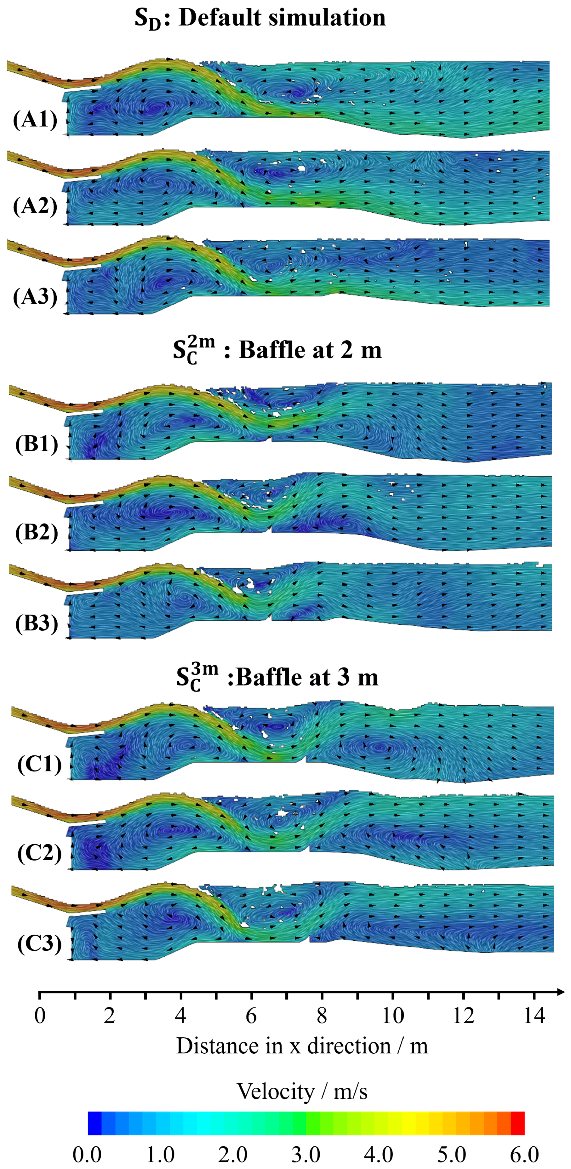
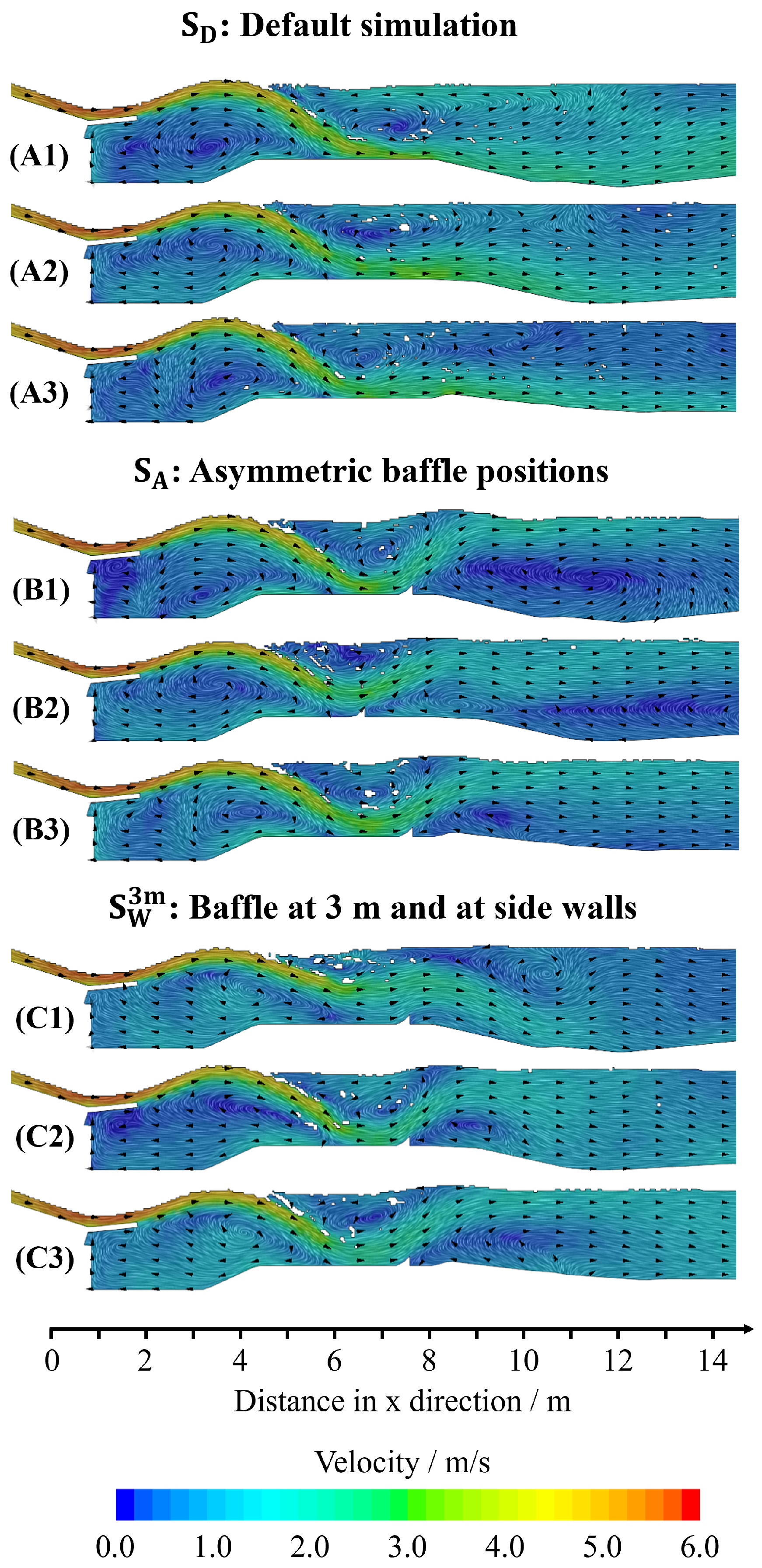
For the investigation of the flow field, three different sections are considered. They are located at 25%, 50%, and 75% of the depth (z direction) of the concrete canal for the simulation volume and represent the land, the middle, and the island sections, respectively. The sections used are visualized in Figure 7 for the simulation volume. Particular care was taken to ensure that the figures accurately represent the flow behavior over time, especially concerning the expansion of the tumble, recurring vortices, and jet behavior, even though the resulting plots represent just one time step. The average simulation time for all simulations was 11:28 h for Setup 1 and 19:00 h for Setup 2.

3.1. Flow Behavior

A comparison of the different variants is conducted using the measured wave height, averaged over the last 5 s, and the value for vorticity for the last iteration. The values for all simulations are summarized in

Table 5. Evaluation of all geometry variants with vorticity $\mathsf{\Psi }$ values of all three space dimensions x, y, z and the wave height. For the configurations, see Figure 3.

Sim.	Name	Wave Height (m)	${\mathbf{\Psi }}_{\mathit{x}}$ ($1/\mathbf{s}·{\mathbf{m}}^3\times {10}^6$)	${\mathbf{\Psi }}_{\mathit{y}}$ ($1/\mathbf{s}·{\mathbf{m}}^3\times {10}^6$)	${\mathbf{\Psi }}_{\mathit{z}}$ ($1/\mathbf{s}·{\mathbf{m}}^3\times {10}^6$)
SCB	$S_D$	0.64	1.27	1.05	4.28
	$S_I$	0.75	1.53	1.01	3.37
	$S_I^{1m}$	0.78	1.42	1.15	3.68
	$S_I^{2m}$	0.76	1.31	1.12	3.21
	$S_I^{3m}$	0.74	1.43	0.91	2.63
	$S_C^{1m}$	0.62	1.20	0.97	3.86
	$S_C^{2m}$	0.65	1.21	0.73	2.07
	$S_C^{3m}$	0.71	1.55	0.75	2.16
ACB	$S_A$	0.64	1.32	0.73	2.04
	$S_{VF}$	0.68	1.30	1.05	2.53
	$S_{VH}$	0.65	1.48	1.01	2.81
SCBW	$S_W$	0.70	1.25	0.87	3.78
	$S_W^{1m}$	0.69	1.14	0.86	3.66
	$S_W^{2m}$	0.76	1.21	0.79	2.48
	$S_W^{3m}$	0.71	1.44	0.70	1.96

. The ${\mathsf{\Psi }}_z$ value is particularly important as it indicates the vorticity of the recirculation zone and resulting tumble in the x and y planes (see Figure 7).

Within the symmetric simulations, we see that different simulation setups do not yield identical ${\mathsf{\Psi }}_y$ values and wave heights across different simulation volumes. This variability is expected due to the non-identical and highly time-dependent flow fields. Geometric changes using a baffle significantly decrease the ${\mathsf{\Psi }}_z$ value. Simulations $S_C^{2m}$ and $S_C^{3m}$ reduce the ${\mathsf{\Psi }}_z$ value by half compared to the default $S_D$ simulation, showing the greatest reduction at a baffle positioned at 2 m. Additionally, ${\mathsf{\Psi }}_y$ decreases for all variants except $S_I^{1m}$ and $S_I^{3m}$, while ${\mathsf{\Psi }}_x$ increases for all variants except $S_C^{1m}$ and $S_C^{2m}$. Most symmetric variants cause the wave height to be greater compared to the default configuration, with the exception of the $S_C^{1m}$ simulation. The 0-1-0 inlay setup $(S_I^{1m},S_I^{2m},S_I^{3m})$ effectively reduces the ${\mathsf{\Psi }}_z$ value but also increases ${\mathsf{\Psi }}_x$ and ${\mathsf{\Psi }}_y$. Conversely, the 1-1-1 inlay setup with baffles $(S_C^{1m},S_C^{2m},S_C^{3m})$ significantly decreases the ${\mathsf{\Psi }}_z$ value with minimal impact on ${\mathsf{\Psi }}_x$. Although the wave height increases, it is not as pronounced as in the 0-1-0 inlay setup. Within the $ACB$ and $SCBW$ groups, most variations perform worse than the $S_C^{2m}$ setup from the symmetric group. Asymmetric baffle configurations ($S_{VF}$ and $S_{VH}$) on the inlay do not lead to improvements. The best performance is observed in the $S_W^{3m}$ simulation, where a combination of baffles at the wall and on the inlay achieves the lowest ${\mathsf{\Psi }}_z$ value with a slight increase in ${\mathsf{\Psi }}_x$. The symmetric baffle configuration $\left(S_A\right)$ setup also performs well in terms of ${\mathsf{\Psi }}_z$ but falls short regarding wave height. The most effective variants are $S_C^{2m}$, $S_C^{3m}$, $S_A$, and $S_W^{3m}$, with the $S_W^{3m}$ setup showing the best results in terms of reducing the recirculation zone, significantly increasing wave height while achieving the lowest ${\mathsf{\Psi }}_z$ value and only a minor drawback in ${\mathsf{\Psi }}_x$. Some general flow features occur independently of the wave module settings, geometric variants or the visualized section. The as-is state, which shows the flow pattern without the usage of a baffle, is visualized in Figure 8(A1–A3). The water accelerates on the wave module and forms a jet, which is directed into the lower water level. After the wave crest (i.e., highest point of the wave), the jet re-enters the water, lowering to the ground and losing velocity. The jet flows along the inlay downstream and spreads out over the entire height of the water. Under the wave crest, a large vortex arises, stabilizing the wave height. The recirculation zone is localized from the point where the water jet re-enters the water until the jet is fully spread out [Figure 8(A1–A3)].

The re-entering process also introduces air into the system. The air bubbles are carried by the current and rise to the water surface, resulting in an upward movement (y direction) in the recirculation zone. Additionally, the re-entering process generates vortices that follow the current along the border of the reflux and the jet on the ground, mostly dissolving at the water surface. In the default simulation $S_D$, we observed that the velocity within the recirculation zone decreases progressively from the land section [Figure 8(A1)] over the center section [Figure 8(A2)] to the island section [Figure 8(A3)]. In comparison, Figure 8(B1–B3) illustrates the influence of a baffle on the flow behavior and the recirculation zone, placed at a distance of 2 m on the inlay. The $S_C^{2m}$ simulation demonstrates that the recirculation zone is significantly affected by the presence of the baffle. The jet is deflected upwards (y direction), reducing the formation of the recirculation zone in all sections. As a result, the recirculation area is shortened to approximately 2 to 3 m. Temporally, in the island section [Figure 8(B3)], the vortices tend to dissolve [Figure 8(B1)], whereas in the land section, the vortices often rise from the ground and remain in their current position. Despite fluctuations, meaning that the smaller recirculation areas detach regularly, the overall wave stability in the $S_C^{2m}$ simulation is maintained. The wave height is comparable across different sections. From the $S_C^{3m}$ simulation, as shown in Figure 8(C1–C3), it is evident that the size of the recirculation zone is directly dependent on the position of the baffle. In simulations $S_C^{2m}$ and $S_C^{3m}$, the baffle is installed after the impact point of the re-entering water jet on the inlay, redirecting the flow and minimizing the recirculation zone. The closer the baffle is to the impact point, the earlier the jet spreads into the water, further reducing the recirculation zone. The temporal behavior differs significantly between simulations $S_C^{2m}$ and $S_C^{3m}$. Simulation $S_C^{2m}$ exhibits vortices forming behind the baffles, which grow, detach, and dissolve in the current. In contrast, simulation $S_C^{3m}$ shows different characteristics across different sections. The land section [Figure 8(C1)] forms a large and stable vortex behind the baffle, resulting in a unique water surface shape due to jet redirection. The center section [Figure 8(C2)] behaves similarly to simulation $S_C^{2m}$, while the island section [Figure 8(C3)] sporadically shows vortices, with cross-sectional currents dominating and preventing vortex formation. Overall, the flow field in simulation $S_C^{3m}$ is more stable over time, whereas the flow field in $S_C^{2m}$ fluctuates constantly. Wave stability is maintained in both simulations, but the wave height increases significantly from 0.65 m in simulation $S_C^{2m}$ to 0.71 m in simulation $S_C^{3m}$.

In comparison to the symmetric simulations (SCB), Figure 9 shows the resulting flow fields for a selected asymmetric simulation with baffles at the bottom and symmetric simulation with baffles at the bottom and walls. The simulated configuration for $S_A$, as shown in Figure 9(B1–B3) combines elements from previous simulations (asymmetric positioning of baffle on the inlay at 2 m and 3 m), leading to a mostly time-stable flow. The center section, however, shows continuous vortex detachments similar to $S_C^{2m}$. The vortex in the land section is significantly expanded compared to $S_C^{3m}$, resulting in a different water surface profile. Other features, such as recirculation zones, vortex behavior, and wave dynamics, align with previous results for their respective sections. In comparison, the simulation setup for $S_W^{3m}$ combines baffles on the inlay at 3 m and the walls. The land and island sections are asymmetric with distinct behaviors. In the land section [Figure 9(C1)], a vertical flow arises from the water surface to the ground, creating an additional vortex behind the baffle. This vertical current redirects the jet back to the inlay. The vortex alternates with the vertical stream, leading to instability. The center and island sections show sporadic vortices that dissolve quickly, similar to previous results. The recirculation zone in the land section is shallow due to early jet spread, while the center and island sections maintain comparable recirculation zones to earlier simulations. Flow behaviors in simulations with diagonal baffles resemble previous results and are not detailed separately.

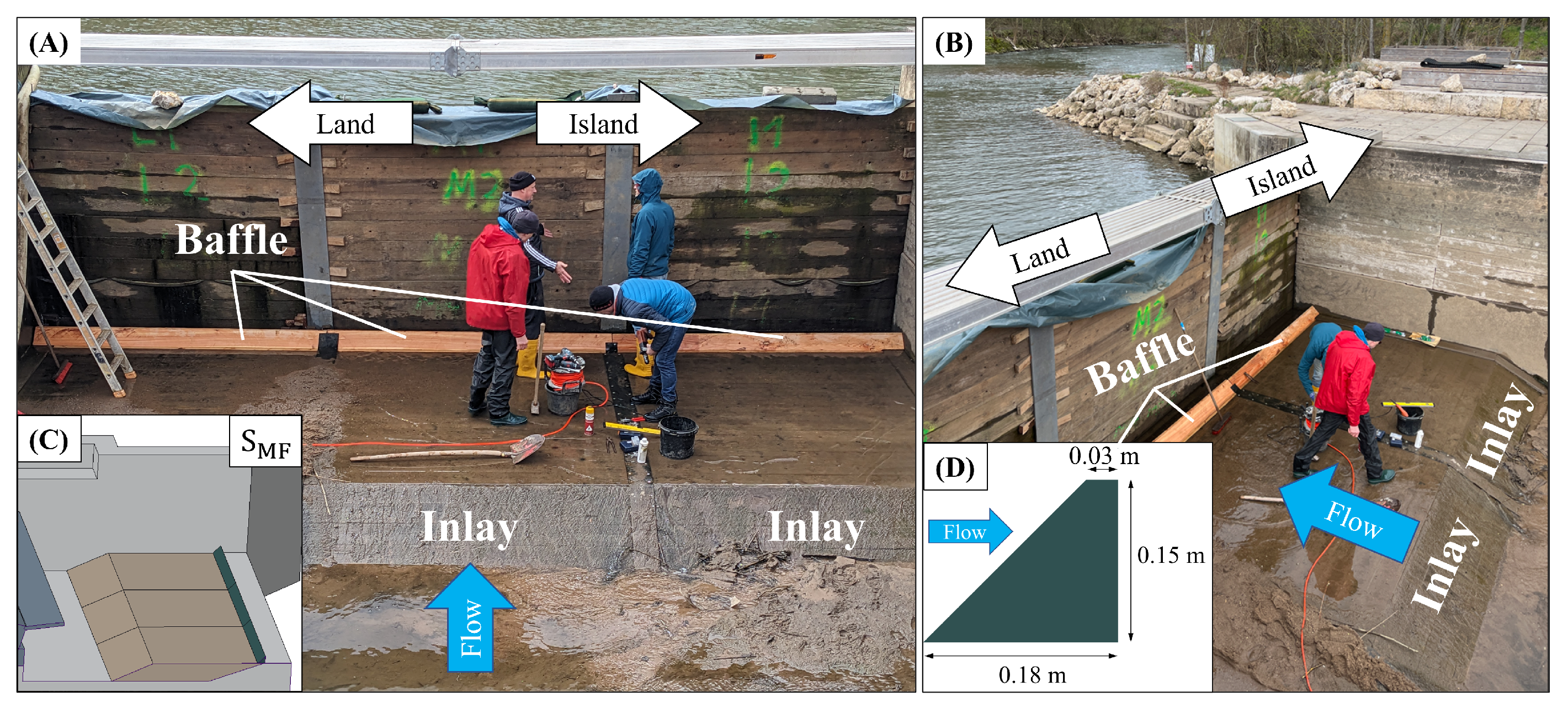
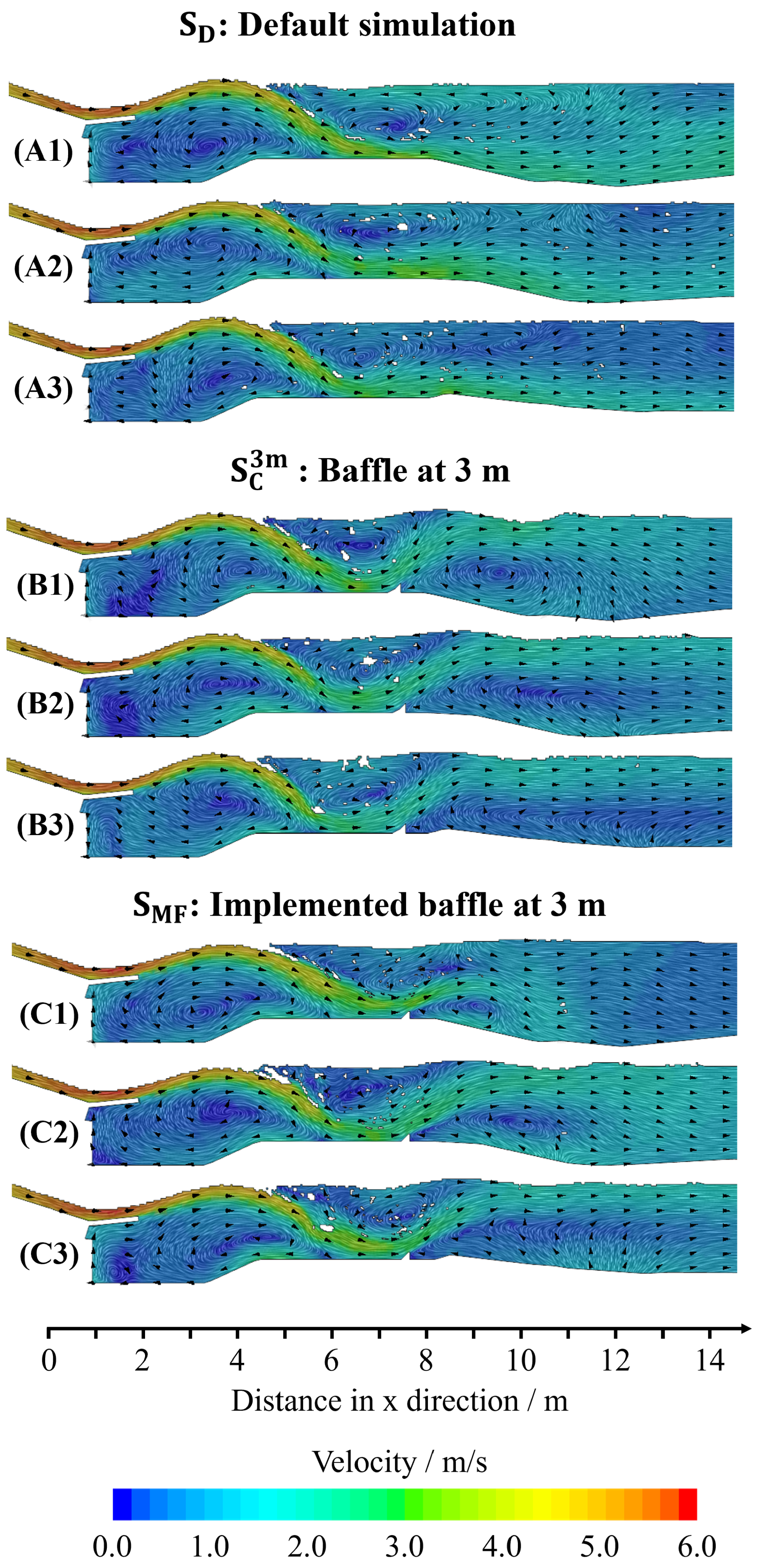
3.2. Real-World Implementation of the Baffle

Based on the presented results, the Nürnberger Dauerwelle e.V. decided to implement a baffle into the actual Fuchslochwelle, which is shown in Figure 10A,B. The used geometry of the real baffle [Figure 10C] was slightly modified in comparison to the baffle geometry used for the simulation [Figure 10D] to facilitate easier manufacturing. The top edge of the baffle was cut off to reduce the risk of injuries for falling surfers. Due to installation constraints, the baffle’s position was fixed at a distance of $l_c$ = 3 m to ensure safe installation and prevent the baffle from being torn out due to water pressure.

To accurately simulate the dimensions of the modified and built-in baffle [Figure 10C], the cell width was limited to a maximum of 3 cm. This refinement around the baffle increased the number of cells in the simulation from approximately $3.5\times {10}^6$ to $6.2\times {10}^6$. The results are presented in Figure 11.

The land section [Figure 11(C1)] shows notable differences to the previous simulations. In $S_{MF}$, instead of the large and stable vortex observed in $S_C^{3m}$, an unstable behavior emerges. The jet is redirected by the baffle but does not reach the water surface. Instead, it is redirected again by a current flowing from the surface to the ground, with the result that the jet ends up in the middle of the water with a tendency toward the ground before spreading upward. The jet remains attached to the vortex behind the baffle, whose center moves over time but never detaches. In the center section of simulation $S_{MF}$ [Figure 11(C2)], the behavior is mostly comparable to the land section of simulation $S_C^{3m}$. A vortex forms behind the baffle, redirecting the jet and creating a distinct water surface shape. This behavior is unstable over time, with the vortex constantly moving. The island section behaves similarly in both simulations, with vortices arising sporadically. The wave height is comparable between both simulations. However, an evaluation of the $\mathsf{\Psi }$ values is not feasible due to the mesh refinement, which leads to an increase in these values as more vorticity vectors are calculated within the same area, resulting in incomparability. Following a two-month test phase with inflows ranging from 5.5 to 10.5 m³/s, the wave operator and surfers provided very positive feedback regarding the system’s performance with the installed baffle. Previously, inflows exceeding 8.5 m³/s created a strong backflow on the water surface behind the wave, leading to challenging and, at times, dangerous situations for less-experienced surfers. Surfers had to either swim vigorously against the backwash or dive beneath it to reach deeper currents and escape the turbulent zone behind the wave. Hence, inflow was limited to 7.5 m³/s water for safety reasons. The introduction of the baffle has substantially mitigated these issues. The modification now allows for the wave to be operated at higher inflows, even above 8.5 m³/s, without the risk of recirculation pulling surfers back into the wave. This adjustment has broadened access of higher inflows to the wave system, making it suitable not only for experienced surfers but also for beginners and first-time surfers, thereby enhancing their safety and overall experience. Hence, inflow up to 9 m³/s can be achieved without any safety concerns, i.e., increase in inflow of 20% considering the previous possible inflow of 7.5 m³/s. To comprehensively assess the impact of the baffle, feedback was collected from a diverse group of surfers, varying in body size, weight, and skill level. This broad range of input was critical for understanding how the modification affected different types of users. Experienced surfers who had previously felt uncomfortable in higher inflows and beginners had no problems exiting the flow area behind the wave with ease. This feedback was pivotal in confirming that the baffle made the wave system safer and more accessible across all skill levels.

Tailwater Dynamics and Areas for Optimization

Here, we refer to the conditions that arise immediately downstream of the wave (the tailwater region) and the ways in which these conditions may be refined to enhance performance and safety. Overall feedback was positive, yet some surfers have mentioned that the tailwater region behind the wave can feel somewhat chaotic due to higher turbulence and increased air entrainment. Under certain conditions, parts of the surface flow may become stagnant, requiring surfers to actively swim out of this zone. Although this situation is considered safe—i.e., there is no risk of being pulled back into the wave—it still represents an opportunity for further optimization. From an ergonomic standpoint, the baffle introduces a slight elevation on the riverbed. However, strong currents near the bottom effectively lift surfers over this obstruction, minimizing the potential for contact. As a result, any risk posed by the baffle is negligible. A secondary issue arises when a surfer reaches the bottom area between the wave and the baffle, where hold-down times can increase slightly. Although there is no significant hold-down or pull-back, and surfers are ultimately carried downstream, this slower flow contrasts with the previous setup, which provided a constant, robust outflow. Adapting to this new dynamic may require some adjustments to be made by surfers and highlights another avenue for refinement. Despite these minor concerns, installing the baffle has markedly improved wave performance and safety, allowing for higher inflows without risking recirculation. This improvement makes the system accessible to surfers of varied skill levels, with overall feedback from those familiar with both configurations being overwhelmingly positive.

3.3. Limitations

The simulation results have not yet been validated through in situ measurements on the actual Fuchslochwelle. Specifically, we have not measured the wave height or the velocities on the wave module, which are used as convergence criteria and for the grid independence study. As a result, we cannot confidently assert that the simulation accurately reflects real-world conditions. Relying on subjective judgment or visual estimation would not provide a sufficient basis for validation. The geometry used in the simulations is a simplified version of the real-world setup. Although this simplification was necessary for computational feasibility, it may not fully capture all the intricacies of the actual environment. For example, the outflow basin, which changes its topology over time, was modeled using a basic measuring method that cannot accurately represent the exact terrain. However, the rocks in the outflow basin move slightly over time due to the constant flow forces. Moreover, the inflow basin was not explicitly modeled; instead, a constant velocity was applied to a simplified rectangular inlet, potentially leading to deviations between simulated and observed flow characteristics. Similarly, the wave module was not precisely modeled but rather approximated in its shape. Furthermore, the area beneath the wave module was closed off in the simulation; however, in reality, this area is open. This could have an effect on the tumble forming the wave and influencing the wave height. These simplifications may introduce uncertainties that could affect the accuracy and applicability of the simulation results. It is important to address this in future simulations for not neglecting potential influences on the overall flow behavior and wave characteristics.

4. Conclusions

In this study, we investigated the impact of geometric modifications to the bottom topology downstream of the wave on the outflow behavior and wave stability of the Fuchslochwelle, an artificial standing wave used for river surfing. A computational fluid dynamics (CFD) simulation in STAR-CCM+ was set up to model various configurations of baffles and inlays to minimize recirculation zones and enhance surfer safety.

• A realistic 3D-CAD model of the Fuchslochwelle was created. A total of 16 configurations were simulated, including both symmetrical and asymmetrical baffle and inlay configurations. The default configuration, intended to represent the current state of the Fuchslochwelle, exhibited similar recirculation patterns to those reported by surfers.
• In the symmetrical group, the reduction in these recirculation zones was most effectively achieved by placing baffles on the inlay at 2 m. In contrast, in the $ACB$ and $SCBW$ groups, recirculation was best minimized by a combination of baffles at the wall and baffles on the inlay at 3 m.
• We simulated a baffle geometry that was subsequently constructed and installed in the Fuchslochwelle. Although this baffle was installed at 3 m rather than the 2 m suggested by the simulations as the optimal placement, it still resulted in a significant reduction in the undesired recirculation zone. This reduction in recirculation was also reported by experienced surfers.
• The results of this study demonstrate that baffles placed on the inlay at 2 m and on the sidewalls can reduce recirculation zones by more than half in terms of vorticity. This approach can be adopted by other wave operators to improve flow conditions in their installations.
• For future work, priority should be given to validation through in situ measurements to further enhance confidence in the presented simulations. Additionally, the impact of geometric simplifications, such as the neglected inflow basin, should be investigated. Lastly, improvements to the numerical setup should be considered to enhance stability, realism, and accuracy.

References

1. Leinewelle, e.V. Surfen mitten in Hannover. 2024. Available online: https://www.enercity-leinewelle.de/ (accessed on 12 February 2025).
2. Nürnberger Dauerwelle e.V. Die FuchslochWelle-SURFEN IN DER STADT. 2024. Available online: https://www.nuernberger-dauerwelle.de/fuchslochwelle/ (accessed on 12 February 2025).
3. Fuchs, H. Effect of adjustable flaps on river surf waves at abrupt drops. In Proceedings of the 37th IAHR World Congress: Learning from the Past for the Future, Kuala Lumpur, Malaysia, 13–18 August 2017; ETH Zurich: Zurich, Switzerland, 2017; p. 7. [Google Scholar] [CrossRef]
4. Hornung, H.G.; Killen, P. A stationary oblique breaking wave for laboratory testing of surfboards. J. Fluid Mech. 1976, 78, 459–480. [Google Scholar] [CrossRef]
5. D’Ambrosio, D. Hydrodynamic Characterization of Planing Surfboards Using CFD. In Proceedings of the 13th Conference of the International Sports Engineering Association, Tokyo, Japan, 22–25 June 2020; p. 68. [Google Scholar] [CrossRef]
6. Oggiano, L. Numerical Comparison between a Modern Surfboard and an Alaia Board using Computational Fluid Dynamics (CFD). In Proceedings of the 5th International Congress on Sport Sciences Research and Technology Support, Funchal, Portugal, 30–31 October 2017; pp. 75–82. [Google Scholar] [CrossRef]
7. Oggiano, L.; Pierella, F. CFD for Surfboards: Comparison between Three Different Designs in Static and Maneuvering Conditions. In Proceedings of the the 12th Conference of the International Sports Engineering Association, Brisbane, Australia, 26–29 March 2018; p. 309. [Google Scholar] [CrossRef]
8. Forsyth, J.R.; Barnsley, G.; Amirghasemi, M.; Barthelemy, J.; Elshahomi, A.; Kosasih, B.; Perez, P.; Beirne, S.; Steele, J.R.; In Het Panhuis, M. Understanding the relationship between surfing performance and fin design. Sci. Rep. 2024, 14, 8734. [Google Scholar] [CrossRef] [PubMed]
9. Falk, S.; Kniesburges, S.; Janka, R.; Grosso, R.; Becker, S.; Semmler, M.; Döllinger, M. Computational hydrodynamics of a typical 3-fin surfboard setup. J. Fluids Struct. 2019, 90, 297–314. [Google Scholar] [CrossRef]
10. Falk, S.; Kniesburges, S.; Janka, R.; O’Keefe, T.; Grosso, R.; Döllinger, M. Numerical Investigation of the Hydrodynamics of Changing Fin Positions within a 4-Fin Surfboard Configuration. Appl. Sci. 2020, 10, 816. [Google Scholar] [CrossRef]
11. Scarfe, B.E.; Elwany, M.H.S.; Mead, S.T.; Black, K.P. The Science of Surfing Waves and Surfing Breaks—A Review; UC San Diego, Scripps Institution of Oceanography: La Jolla, CA, USA, 2003. [Google Scholar]
12. Antunes Do Carmo, J.S.; Neves, M.G.; Ten Voorde, M. Designing a multifunctional artificial reef: Studies on the influence of parameters with most influence in the vertical plane. J. Coast. Conserv. 2011, 15, 99–112. [Google Scholar] [CrossRef]
13. Black, K.; Mead, S. Design of Surfing Reefs. Reef J. 2009, 1, 177–191. [Google Scholar]
14. Cáceres, I.; Trung, L.H.; Dirk Van Ettinger, H.; Reniers, A.; Uijttewaal, W. Wave and Flow Response to an Artificial Surf Reef: Laboratory Measurements. J. Hydraul. Eng. 2010, 136, 299–310. [Google Scholar] [CrossRef]
15. Ten Voorde, M.; Do Carmo, J.S.A.; Neves, M.G. Designing a Preliminary Multifunctional Artificial Reef to Protect the Portuguese Coast. J. Coast. Res. 2009, 251, 69–79. [Google Scholar] [CrossRef]
16. Hager, W.H.; Bretz, N.V. Hydraulic jumps at positive and negative steps. J. Hydraul. Res. 1986, 24, 237–253. [Google Scholar] [CrossRef]
17. Kawagoshi, N.; Hager, W.H. Wave type flow at abrupt drops: I. Flow geometry. J. Hydraul. Res. 1990, 28, 235–252. [Google Scholar] [CrossRef]
18. Moore, W.L.; Morgan, C.W. Hydraulic Jump at An Abrupt Drop. Trans. Am. Soc. Civ. Eng. 1959, 124, 507–516. [Google Scholar] [CrossRef]
19. Mossa, M.; Petrillo, A.; Chanson, H. Tailwater level effects on flow conditions at an abrupt drop. J. Hydraul. Res. 2003, 41, 39–51. [Google Scholar] [CrossRef]
20. Ohtsu, I.; Yasuda, Y. Transition from supercritical to subcritical flow at an abrupt drop. J. Hydraul. Res. 1991, 29, 309–328. [Google Scholar] [CrossRef]
21. Rajaratnam, N.; Ortiz, N.V. Hydraulic Jumps and Waves at Abrupt Drops. J. Hydraul. Div. 1977, 103, 381–394. [Google Scholar] [CrossRef]
22. Oertel, M.; Mönkemöller, J.; Schlenkhoff, A. Artificial stationary breaking surf waves in a physical and numerical model. J. Hydraul. Res. 2012, 50, 338–343. [Google Scholar] [CrossRef]
23. Borman, D.J.; Sleigh, P.A.; Coughtrie, A.; Horton, L. Hydraulic Free-Surface Modelling with a Novel Validation Approach. In Proceedings of the 9th South African Conference on Computational and Applied Mechanics, Somerset West, South Africa, 14–16 January 2014. [Google Scholar]
24. Asiaban, P.; Rennie, C.D.; Egsgard, N. Sensitivity Analysis of Adjustable River Surf Waves in the Absence of Channel Drop. Water 2021, 13, 1287. [Google Scholar] [CrossRef]
25. Hirt, C.; Nichols, B. Volume of fluid (VOF) method for the dynamics of free boundaries. J. Comput. Phys. 1981, 39, 201–225. [Google Scholar] [CrossRef]
26. Menter, F.R. Two-equation eddy-viscosity turbulence models for engineering applications. AIAA J. 1994, 32, 1598–1605. [Google Scholar] [CrossRef]
27. Wilcox, D.C. Reassessment of the scale-determining equation for advanced turbulence models. AIAA J. 1988, 26, 1299–1310. [Google Scholar] [CrossRef]
Figure 1. Exemplary surf wave illustration showing four distinct flow regions, inflow, surf wave, recirculation zone, and outflow, from (A) side view and (B) top view, with light blue arrows indicating flow direction, a dark blue vortex representing wave stabilization, and a red vortex depicting the undesired tumbling effect [3].
Applsci 15 03127 g001
Figure 2. The figure shows a (A) satellite picture of the Fuchslochwelle with the inflow basin, the concrete canal and outflow basin; (B) the wave module and inlay within the concrete canal; and (C) CAD model of the Fuchslochwelle: (1) inflow basin, (2) concrete canal, (3) outflow basin, (4) wave module, (5) inlay, and (6) potential baffle. (D) Schematic CAD view of the primary variables for various geometry variants, featuring different configurations of the wave module (gray), inlays (beige), and baffle (dark green). The blue plane represents the water level at the inlet, while the green plane indicates the water level at the outlet. The flow direction of the water is illustrated by the light blue arrow. The physical values for the simulations are further detailed in Table 1. Subfigure (E) shows the geometry of the installed baffle with its dimensions shown in meters.
Applsci 15 03127 g002
Figure 3. The figure shows different variants of (A1A8) symmetric with baffles at the bottom (SCB); (B1B4) symmetric with baffles at the bottom and side walls (SCBW); and (C1C3) asymmetric baffle at the bottom (ACB) inlay (beige) and baffle (green) positions. In (B1B4), side wall baffles are depicted on one side for illustration purposes; however, in the simulations, they were implemented on both sides.
Applsci 15 03127 g003
Figure 4. Boundary conditions for the simulation volume: Red indicates the velocity inlet and outlet, gray represents the no-slip wall, and orange denotes the pressure boundary.
Applsci 15 03127 g004
Figure 5. Visualization of probe locations for velocity measurements (1–4, red dots) and the wave height measurement (5, black line), which were selected to facilitate validation. The light blue arrow indicates the flow direction.
Applsci 15 03127 g005
Figure 6. (A) Vorticity calculation volume V t m b l (green), measuring 10 m in length and 8 m in width, encompassing all cells below the water surface. (B) The image illustrates the rotational components of vorticity Ψ x (blue), Ψ y (red), and Ψ z (green) in their respective planes within the three-dimensional space. The rotating arrows indicate the direction and sense of rotation of the components in the x, y, and z directions, corresponding to the orientation of the coordinate system shown in the upper left corner. Part (1) indicates the wave module, part (2) represents the concrete canal, and part (3) represents the inlay.
Applsci 15 03127 g006
Figure 7. Visualization of the localization of the sections for a further velocity flow field presentation. The sections are positioned at 25% (land), 50% (middle), and 75% (island) of the depth of the concrete canal.
Applsci 15 03127 g007
Figure 8. The figure shows the velocity flow field comparison for (A1A3) for the default configuration ( S D ); (B1B3) for the configuration with baffles positioned at 2 m ( S C 2 m ); and (C1C3) the configuration with baffles at 3 m ( S C 3 m ). Sections (1, 2, 3) represent land, middle, and island, respectively, as shown in Figure 7.
Applsci 15 03127 g008
Figure 9. The figure shows the velocity flow field comparison for (A1A3) for the default configuration ( S D ); (B1B3) for the configuration with asymmetric baffle positions ( S A ); and (C1C3) the configuration with baffles at 3 m and at the side walls ( S W 3 m ). Sections (1, 2, 3) represent land, middle, and island, respectively, as shown in Figure 7.
Applsci 15 03127 g009
Figure 10. The actual (A,B) Fuchslochwelle is shown in a drained condition in which the baffle is implemented. Subfigures (C,D) show the geometry of the installed baffle with its dimensions.
Applsci 15 03127 g010
Figure 11. The figure shows the velocity flow field comparison for (A1A3) for the default configuration ( S D ); (B1B3) for the configuration with baffles positioned at 2 m ( S C 3 m ); and (C1C3) for the configuration with baffles at 3 m ( S M F ). Sections (1, 2, 3) represent land, middle, and island, respectively, as shown in Figure 7.
Applsci 15 03127 g011