A Hybrid Deep Learning Approach for Integrating Transient Electromagnetic and Magnetic Data to Enhance Subsurface Anomaly Detection

Abstract

Recent advancements in geophysical exploration have highlighted the importance of integrating electromagnetic (EM) and magnetic data to enhance subsurface target detection. Conventional inversion techniques often struggle with the non-uniqueness of solutions and sensitivity to noise when relying on a single data modality. In this study, we introduce a novel deep learning framework, MagEMNet, designed to jointly invert EM and magnetic responses. This convolutional neural network (CNN)-based model effectively combines these two complementary data types, improving the estimation of target characteristics such as location, orientation, and physical properties. Trained on synthetic datasets generated through forward modeling, MagEMNet leverages the adaptive moment estimation (Adam) optimizer and a dynamic learning rate strategy to enhance convergence. Our results show that MagEMNet not only outperforms traditional inversion techniques in terms of accuracy but also accelerates the inversion process, offering an efficient solution for real-world applications, including unexploded ordnance (UXO) detection and subsurface resource assessment.

1. Introduction

In recent years, electromagnetic (EM) and magnetic methods have been essential in geophysical exploration, widely applied in subsurface detection for identifying targets with varying electrical and magnetic properties [1,2,3,4]. However, traditional inversion techniques face significant limitations, including susceptibility to local minima and dependence on initial values, which can lead to inaccurate results. These challenges are further compounded by the non-uniqueness of solutions, a common issue when using single-type geophysical data [5,6,7]. Specifically, transient electromagnetic (TEM) methods effectively capture conductivity variations but are limited in depth penetration, while magnetic methods excel in detecting deeply buried ferromagnetic targets but are often hindered by geological noise [7,8,9].

To overcome these challenges, joint inversion approaches, which integrate data from multiple geophysical modalities, have been developed [10,11,12,13,14]. These methodologies capitalize on the complementary nature of EM and magnetic responses, thereby enabling the derivation of more constrained and reliable subsurface models. Joint inversion techniques can be broadly categorized into two frameworks: those based on empirical relationships between physical properties and those relying on spatial distribution coupling. The former assumes predefined relationships, such as the correlation between resistivity and density, and has been successfully applied to the joint inversion of electromagnetic, seismic, and gravity data [15]. However, these methods are often limited by the variability of such relationships across different geological contexts. The latter, on the other hand, eliminates the need for direct correlation by employing structural coupling, such as cross-gradient functions, to achieve spatially coherent inversions. This approach has been effectively demonstrated in the integration of gravity and magnetic datasets [9].

Joint inversion methodologies, which integrate data from multiple geophysical sources, have emerged to overcome these limitations. By leveraging the complementary nature of EM and magnetic responses, joint inversion approaches provide a more constrained and reliable subsurface model, improving both the accuracy and robustness of inversion results. Pasion et al. [8] demonstrated that combining magnetic and TEM data enables more effective target discrimination, especially in applications such as unexploded ordnance (UXO) detection, where traditional methods may struggle due to environmental noise and complex subsurface interactions. Zhang and Wang [9] further highlighted that integrating gravity and magnetic data using cross-gradient joint inversion significantly reduces the ill-posedness inherent in single-method inversions, offering a more stable solution for complex geological settings. Abubakar et al. [5] showed that combining EM with elastic data enhances the inversion’s robustness, allowing for a more comprehensive understanding of the subsurface by incorporating both electrical and mechanical properties. The effectiveness of joint inversion has been further validated in a range of geophysical applications, showing improved robustness and stability compared to traditional methods [16].

Among various applications of magnetic data inversion, unexploded ordnance (UXO) detection is a prominent example. The following studies provide insights into advancements and limitations in this domain: Magnetic data inversion has been extensively studied in the context of UXO detection. For example, Sanchez et al. [17] highlighted the importance of magnetic moments in UXO clearance, while Maha Abdelazeem and Gobashy [18] proposed a Kaczmarz regularization-based approach to address magnetic anomaly inversion. Furthermore, Butler [19] and Butler et al. [20] investigated the impact of magnetic backgrounds and multisensor methods for UXO detection, providing valuable insights into the challenges of signal discrimination and data fusion. Although these traditional approaches have advanced UXO detection, they often rely on regularization or sequential constrained inversion, which can be limited when dealing with highly complex geological settings. In contrast, the framework proposed in this study integrates TEM and magnetic data through a deep learning paradigm, enabling simultaneous data fusion and leveraging the strong generalization capacity of convolutional neural networks (CNNs) to improve both accuracy and robustness in joint inversion.

Recent advancements in deep learning (DL) have enabled further innovation in geophysical inversion. Deep neural networks (DNNs), particularly CNNs, offer powerful tools for analyzing complex data relationships in joint inversion tasks. Algorithms such as CNNs have demonstrated remarkable potential in solving complex geophysical problems, including one-dimensional inversion of electromagnetic data [21,22], structural interpretation of seismic images [23], and magnetization direction prediction [24]. CNNs have also been employed for gravity inversion tasks, including depth-to-basement prediction [25] and three-dimensional gravity analysis [26]. Li et al. [7] showcased the potential of DL-based inversion techniques for subsurface EMI response, achieving faster and more accurate inversion results compared to traditional algorithms. However, ML-based methods are not without challenges; the scarcity of high-quality training datasets often restricts their generalizability, posing a significant obstacle to their widespread application [27]. Building on this foundation, we propose MagEMNet, a CNN-based joint inversion framework designed to integrate both electromagnetic induction (EMI) and magnetic field data. This approach leverages adaptive moment estimation (Adam) [28] and a learning rate decay strategy to optimize convergence and enhance the model’s predictive accuracy.

By simultaneously incorporating EMI and magnetic datasets, MagEMNet addresses the limitations of single-method inversions and captures the interrelationships between different geophysical properties, resulting in a more comprehensive understanding of subsurface targets. Simulated and field experiments demonstrate that our framework not only improves inversion accuracy but also significantly accelerates computational speed, providing a practical and efficient solution for applications such as UXO detection and subsurface resource exploration.

Our key contributions can be succinctly summarized as follows:

(1)

Proposing a Unified Deep Learning Framework for Joint Inversion: We developed MagEMNet, a CNN-based model tailored for the joint inversion of electromagnetic (EM) and magnetic data. By leveraging the complementary nature of these two modalities, MagEMNet achieves higher accuracy and robustness compared to traditional single-modality methods, addressing challenges such as non-uniqueness and noise susceptibility.

(2)

Innovative Integration of Physics-Constrained Learning and Advanced Deep Learning Architectures: The framework incorporates Squeeze-and-Excitation (SE) blocks [29] to enhance feature selection and a physics-constrained loss function to ensure physical consistency in inversion results. This integration significantly improves the reliability of parameter recovery while preserving interpretability and adherence to geophysical principles.

(3)

Comprehensive Validation Through Synthetic and Field Experiments: The study presents rigorous evaluations of MagEMNet using a large-scale synthetic dataset generated from a three-dimensional orthogonal magnetic dipole model. Field experiments further demonstrate the model’s practical applicability, with results showing depth errors of less than 10 cm and efficient inversion of target parameters.

This paper is organized as follows. Section 2 introduces the integrated detection framework, detailing the structures and functionalities of the unmanned aerial vehicle magnetic (UAVMAG) and the unmanned aerial vehicle time-domain electromagnetic (UAV-TDEM) systems. Section 3 describes the proposed MagEMNet framework, including its CNN-based architecture, physics-constrained loss function, and the forward modeling techniques utilized for synthetic data generation. Section 4 presents the experimental results, including comprehensive synthetic and field evaluations, along with comparisons against traditional inversion methods. Finally, Section 5 concludes the study and outlines directions for future research.

2. System

The integrated detection framework combines the unmanned aerial vehicle magnetic (UAVMAG) measurement system and the unmanned aerial vehicle time-domain electromagnetic (UAV-TDEM) detection system, operating sequentially to prevent mutual interference. Both systems are equipped with RTK GPS, specifically the T300 unit, manufactured by Shanghai Sinan Satellite Navigation Technology Co., Ltd. (Shanghai, China), which provides centimeter-level positioning accuracy and delivers timing precision up to 20 ns (pulse per second, pps). The RTK GPS ensures precise spatial registration within a unified coordinate framework, enabling high-fidelity synchronization between magnetic and electromagnetic measurements.

2.1. UAV-TDEM System

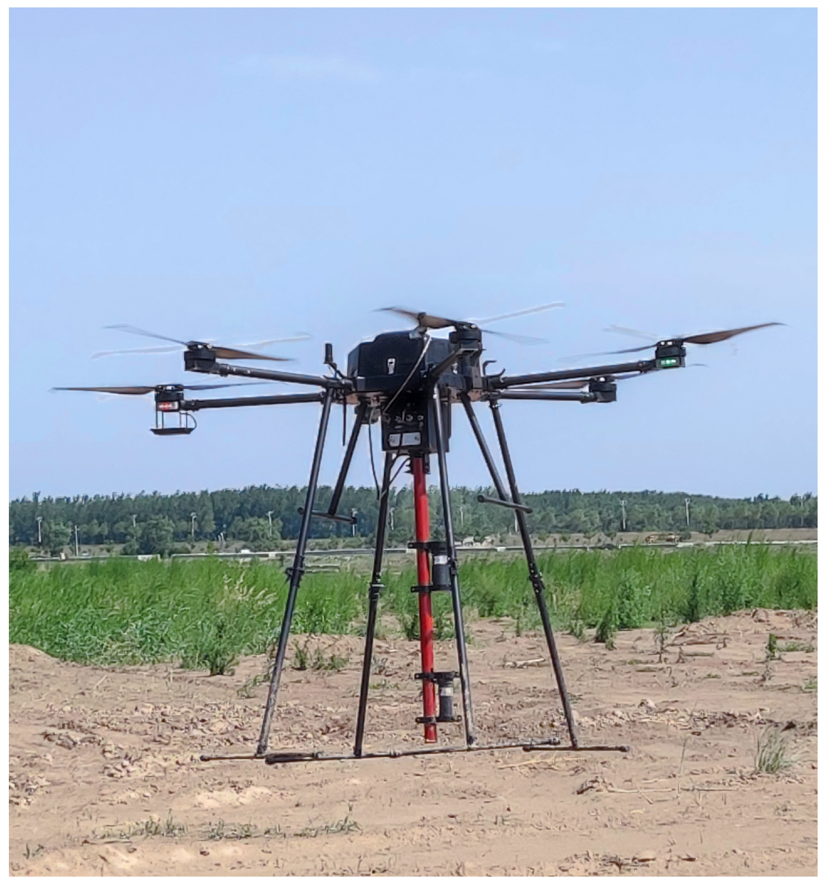
The UAV-TDEM system is meticulously designed for efficient and high-resolution subsurface exploration, particularly for detecting shallow targets. The architecture incorporates a sophisticated UAV platform, a host control system, and electromagnetic transceiver sensors, working in concert to accurately capture electromagnetic field data. Real-time georeferencing through RTK GPS technology ensures spatial synchronization. Figure 1 presents the structural layout of the UAV-TDEM system.

The UAV platform forms the foundation of the system, offering stability and precision in navigation, both of which are essential for achieving high-quality data in extensive survey missions. Following comprehensive performance evaluations, a six-rotor UAV from Sunward Technology Co., Ltd. (Zhuzhou, China) was selected, distinguished by its payload capacity, stability, and reliability under survey conditions. This UAV can support sustained flight with a considerable payload for up to 40 min, enabling efficient, large-scale surveys in a single mission.

The host system within the UAV-TDEM setup consists of a control module, transmitter, and data acquisition module. The control module oversees signal generation and data collection timing, transmitting commands to adjust frequency and timing settings. This coordination ensures synchronized operations between the UAV’s flight and the data acquisition process, maintaining precise control over the electromagnetic data capture.

The transmitter employs an H-bridge circuit to manage current direction within the transmitting coil, creating a bipolar waveform to produce a consistent primary magnetic field with a maximum current output of 8 A. Once transmission ceases, the receiver captures the secondary field generated by eddy currents within subsurface anomalies. The data acquisition module then amplifies and digitizes the signals, with onboard storage for post-processing. Real-time data visualization is available via Wi-Fi connection to a base station, allowing immediate quality control and data validation during field operations.

The transceiver sensor array includes a 1 m × 1 m transmitting coil for primary magnetic field generation and a 0.5 m × 0.5 m receiving coil to capture the induced secondary field. The receiving coil operates with a high bandwidth of 140 kHz, ensuring precise transient response measurements essential for characterizing subsurface anomalies. Advanced signal processing features, such as low-pass filtering and analog-to-digital conversion, enhance data accuracy by reducing noise. The RTK GPS integration further ensures precise geospatial alignment, providing centimeter-level accuracy critical for spatially synchronized measurements.

The transceiver sensor array is suspended from the UAV via non-magnetic nylon ropes to mitigate interference from the UAV’s frame and electronic components. This suspension mechanism significantly reduces platform-induced noise, isolating the electromagnetic response of shallow subsurface targets. The UAV’s flight path is programmed to maintain a 0.5 m line spacing at a controlled speed of 1 m/s, ensuring data consistency and high lateral resolution across the survey area.

2.2. UAVMAG System

The UAVMAG system is tailored for high-resolution magnetic field measurements aimed at subsurface anomaly detection, such as unexploded ordnance (UXO) and geological structures. It integrates a high-sensitivity magnetometer array, RTK GPS, and a specialized UAV platform to ensure precise spatial positioning and accurate magnetic data capture. Figure 2 presents the structural layout of the UAVMAG system.

To reduce platform-induced magnetic interference, the magnetometers are attached to a rigid vertical suspension boom beneath the UAV, secured with non-magnetic, non-conductive nylon connectors. This configuration minimizes magnetic noise by distancing the sensors from potential sources of interference, allowing the magnetometers to detect subsurface-related magnetic signals without significant contamination from the UAV’s electronic and structural components.

The suspended sensor assembly maintains a stable orientation relative to the ground during flight, enabling consistent magnetic data acquisition even as the UAV maneuvers along its flight path. The UAV follows a pre-programmed survey route with a line spacing of 0.5 m and a speed of 1 m/s, achieving high-resolution magnetic data collection across the survey grid.

The magnetic sensor suite includes two high-precision magnetometers designed for capturing both scalar and vector magnetic field components. The Mag-03MS1000 magnetometer, with a range of $\pm 70$, $\pm 100$, $\pm 250$, $\pm 500$, and $\pm 1000\mathrm{\mu }\mathrm{T}$, provides noise levels as low as 6–$10\mathrm{pT}/\sqrt{\mathrm{Hz}}$ at $1\mathrm{Hz}$. Its compact dimensions ($32\times 32\times 152\mathrm{mm}$) and lightweight design ($0.16\mathrm{kg}$) make it ideal for UAV-based applications where weight is a constraint. Complementing this sensor is the CAS-18-VL magnetometer, which extends the measurement range to $10,000$–$105,000\mathrm{nT}$ with a noise sensitivity of $0.3\mathrm{pT}/\sqrt{\mathrm{Hz}}$ at $1\mathrm{Hz}$. The CAS-18-VL’s dimensions ($53\mathrm{mm}$ in diameter and $130\mathrm{mm}$ in length) and weight ($0.5\mathrm{kg}$) make it suited for high-intensity magnetic surveys, providing a robust detection capability for a wide range of anomaly intensities.

To facilitate readers in quickly understanding the specific parameters of the system, we present the technical specifications of the UAVMAG system, as shown in

Table 1. The technical specifications of the UAVMAG system.

Module	Technical Index	Specifications
UAV	Flight speed	14 m/s, maximum air speed; 2–4 m/s, recommended speed
	Mass of payload	10 kg, maximum payload; 5 kg, standard payload
	Takeoff weight	19 kg, standard
	Endurance	35 min with a payload of 5 kg
Magnetic sensors	CAS-18-VL	Operating range: 10,000 nT to 105,000 nT
		Noise sensitivity: 0.3 pT/$\sqrt{\mathrm{Hz}}$ @ 1 Hz
	Mag-03MS1000	Operating range: ±100 nT
		Noise sensitivity: 4 pT/Hz @ 1 Hz
Power	Data acquisition module	3200 mAh lithium polymer battery; voltage: 24 V

.

Both magnetometers are synchronized with the UAV’s RTK GPS, ensuring spatial alignment of magnetic readings with precise positional data. The RTK GPS offers centimeter-level positioning accuracy, crucial for high-resolution mapping of magnetic anomalies, and enables the integration of magnetic data with geospatial coordinates, facilitating comprehensive anomaly characterization.

The data acquisition module operates at a high sampling rate of 160 Hz, capturing subtle magnetic field variations that indicate the presence of subsurface ferromagnetic materials. The acquired magnetic field signal consists of the geomagnetic field, UAV interference magnetic field, and magnetic anomaly signal. Within a small area, the geomagnetic field remains approximately stable over short periods and spatially uniform [30]. To eliminate its influence, the DC component is removed, while the UAV interference magnetic field is suppressed using the LTI model proposed by other members of our laboratory, as detailed in reference [31]. Additionally, this module includes real-time filtering capabilities to mitigate high-frequency noise and other unwanted interference. Post-processing techniques further enhance data integrity, effectively isolating target-related magnetic anomalies for accurate interpretation.

In summary, the UAVMAG system integrates high-sensitivity magnetometers and precise spatial control, making it a versatile tool for detecting shallow subsurface magnetic anomalies across large survey areas. Its robust design and advanced positioning technology make it suitable for applications such as UXO detection, geological surveying, and environmental monitoring, providing a reliable solution for remote sensing tasks that require both high accuracy and operational efficiency.

3. Materials and Methods

3.1. Electromagnetic and Magnetic Field Response Modeling

In geophysical exploration, both electromagnetic (EM) and magnetic methods are utilized to investigate subsurface properties by detecting contrasts in conductivity and magnetization, respectively. In this study, a dipole model is employed for both EM and magnetic forward modeling, allowing for a unified and consistent description of the target’s response across both modalities. The magnetic polarizability tensor (MPT) serves as the principal descriptor of the target’s intrinsic magnetization properties, ensuring that the EM and magnetic responses can be coherently integrated.

3.1.1. Electromagnetic Forward Modeling

The time-domain electromagnetic (TEM) method is widely used to detect conductive anomalies in the subsurface. This method operates by generating primary magnetic fields that induce eddy currents within conductive targets, which in turn produce secondary magnetic fields that decay over time. Under far-field conditions—where the distance between the sensor and the target significantly exceeds the target’s dimensions—the secondary field response can be approximated by a 3D orthogonal magnetic dipole model, which simplifies the complex response of the target into three independent magnetic dipole components oriented along orthogonal axes, represented by the intrinsic magnetic dipole strength $L_1$, $L_2$, and $L_3$ [7,32].

The induced magnetic moment $\overrightarrow{m}\left(r_T\right)$ at the target location $r_T$ can be expressed as follows:

$$\overrightarrow{m}\left(r_T\right)={\displaystyle \frac{2\pi }{{\mu }_0}}M·{\overrightarrow{B}}_T\left(r_T\right),$$

(1)

where ${\overrightarrow{B}}_T$ is the primary magnetic field at the target location, ${\mu }_0$ denotes the permeability of free space, and M is the magnetic polarizability tensor (MPT) that describes the target’s anisotropic magnetization response in its local coordinate system. The MPT M is represented as follows:

$$M=U\left[\begin{array}{ccc}{L}_1& 0& 0\\ 0& L_2& 0\\ 0& 0& L_3\end{array}\right]U^T,$$

(2)

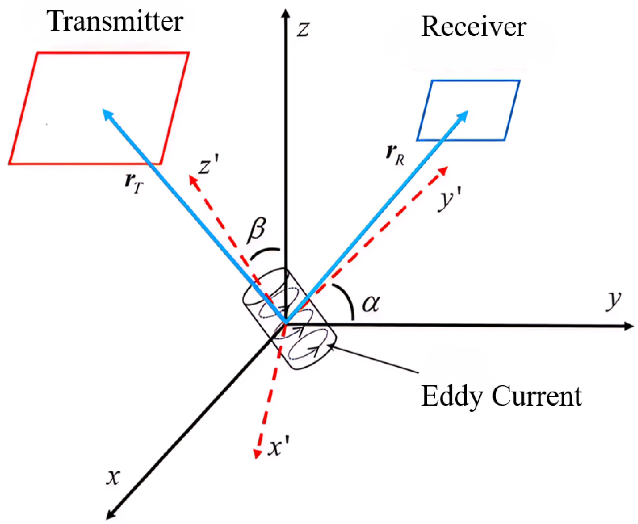
where $L_1$, $L_2$, and $L_3$ are the principal magnetic polarizability components along each orthogonal axis. Due to the axial symmetry of the problem, the rotation matrix U aligns the local coordinate system of the target with the global coordinate system and is defined as follows:

$$U=\left[\begin{array}{ccc}cos\alpha cos\beta & sin\alpha cos\beta & -sin\beta \\ -sin\alpha & cos\alpha & 0\\ cos\alpha sin\beta & sin\alpha sin\beta & cos\beta \end{array}\right],$$

(3)

where $\alpha$ and $\beta$ are the azimuth and dip angles, respectively, which specify the target’s orientation in space.

To fully illustrate the relationship between the local coordinate system of the object and the global coordinate system, we provide a schematic diagram of the dipole model, as shown in Figure 3.

The total secondary field response F of the three orthogonal dipole components can be expressed as the sum of the responses generated by each component. Based on the forward model, we define the response as follows:

$$F(r_T,r_R)=\sum _{i=1}^3{F}_i(r_T,r_R)=\sum _{i=1}^3{\displaystyle \frac{{\mu }_0}{4\pi |r_R{|}^3}}{m}_i·\left[{\displaystyle \frac{3r_R{r}_R^T}{|r_R{|}^2}}-\mathbf{I}\right],$$

(4)

where

• $r_T$ and $r_R$ denote the positions of the target and receiver, respectively.
• $F_i(r_T,r_R)$ represents the secondary field response from each orthogonal dipole component (i.e., $i=1,2,3$).
• ${\mu }_0$ is the permeability of free space.
• $m_i$ denotes the intrinsic dipole strengths in the i-th direction, specifically $L_1$, $L_2$, and $L_3$ corresponding to the three orthogonal dipole components.
• $r_R{r}_R^T$ is the outer product of the receiver position vector ${\mathbf{r}}_R$, forming a matrix.
• $\mathbf{I}$ is the identity matrix, ensuring the response considers both radial and angular components of the field generated by each dipole orientation.

This formulation captures the combined secondary field response as the sum of contributions from each of the three orthogonal dipole components, characterized by the target parameters $(x,y,z,L_1,L_2,L_3,\alpha ,\beta )$. Here, $\alpha$ and $\beta$ represent the rotation and inclination angles of the dipole orientations relative to the coordinate system, which affects the directional response of each component.

This unified expression allows the model to calculate the total secondary field response at the receiver position, given the dipole parameters and orientation angles. This response formula serves as a critical component for forward modeling, forming the basis of synthetic data generation used for training and validating inversion models in electromagnetic and magnetic field analysis.

3.1.2. Magnetic Forward Modeling

The magnetic method similarly employs a dipole model to capture the static magnetic field generated by the target. In this case, the target is treated as a magnetic dipole with an effective magnetic moment that aligns with the target’s principal magnetic response axes, which are characterized by the same magnetic polarizability tensor M used in TEM modeling. This approach ensures that the EM and magnetic forward models maintain a unified physical description of the target’s magnetization properties.

The static magnetic field ${\overrightarrow{B}}_M$ observed at an observation point $\overrightarrow{r}$ relative to the target can be represented as follows:

$${\overrightarrow{B}}_M={\displaystyle \frac{{\mu }_0}{4\pi }}\left({\displaystyle \frac{3({\overrightarrow{m}}_{\mathrm{eff}}·\overrightarrow{r})\overrightarrow{r}}{|\overrightarrow{r}{|}^5}}-{\displaystyle \frac{{\overrightarrow{m}}_{\mathrm{eff}}}{|\overrightarrow{r}{|}^3}}\right)$$

(5)

where the effective magnetic moment ${\overrightarrow{m}}_{\mathrm{eff}}$ is defined as

$${\overrightarrow{m}}_{\mathrm{eff}}={\displaystyle \frac{2\pi }{{\mu }_0}}M·{\overrightarrow{B}}_{earth}$$

(6)

By utilizing the same magnetic polarizability tensor M across both EM and magnetic models, the static magnetic response aligns with the transient response in the TEM model, thereby achieving a consistent description of the target’s physical properties.

In this study, we assume that the magnetic response is dominated by induced magnetization rather than remanent magnetization. This assumption is based on prior research in UXO detection, which has shown that most UXO undergo significant demagnetization due to mechanical shocks and high-temperature exposure during manufacturing or detonation [33,34,35]. Consequently, remanent magnetization is often negligible compared to induced magnetization in practical detection scenarios.

3.1.3. Unified Modeling and Consistency Verification

Both the electromagnetic and magnetic field responses are governed by the magnetic polarizability tensor M, ensuring a consistent physical representation of the target’s magnetization across both methods. While TEM modeling captures the time-decaying secondary EM field, magnetic modeling provides a static magnetic field representation. By employing a shared MPT and the effective magnetic moment formulation, both forward models converge within a single, unified framework, enabling integrated analysis and enhancing the robustness of inversion results.

3.2. Synthetic Dataset Generation

To effectively train the deep learning-based inversion model, a comprehensive synthetic dataset was generated using a forward modeling approach based on a three-dimensional orthogonal magnetic dipole model. These synthetic data simulate the electromagnetic and magnetic field responses of various subsurface targets, thereby allowing the network to learn diverse scenarios and achieve generalization to complex geological environments.

To avoid the issue of non-uniqueness in the inversion process—where different parameter combinations could yield similar responses—the range of target parameters was carefully constrained in accordance with the specific experimental setup.

Table 2. Parameter range of forward model.

Parameter	Range	Spacing	Unit
x	[3.5, 6.5]	0.01	m
y	[3.5, 6.5]	0.01	m
z	[−3, −0.5]	0.01	m
$\alpha$	(0, 360)	1	degree
$\beta$	(0, 90)	1	degree
$L_1$	[0.1, 10]	0.01	-
$L_2$	[0.1, 10]	0.01	-
$L_3$	[1, 100]	1	-

illustrates the predefined ranges for each parameter, including spatial coordinates $(x,y,z)$, magnetic polarizability values $(L_1,L_2,L_3)$, and orientation angles $(\alpha ,\beta )$.

The data acquisition was conducted over an observation plane positioned above the target area, as depicted in Figure 4. This plane contains 49 measurement points arranged in a grid format, with a 0.5 m spacing between each point, covering a total area of 3.5 m ∗ 6.5 m. The target parameters were generated based on systematic rules, allowing variations in spatial location, orientation, and polarizability. For each parameter set, the forward model simulated both the electromagnetic response and the magnetic field response at the observation points. To improve the model’s robustness, a noise level of 5% was added to each simulated magnetic anomaly response, rather than the total geomagnetic field, ensuring that the introduced perturbation accurately represents realistic measurement uncertainties encountered in practical surveys. This approach enhances the generalization capability of the inversion network.

The synthetic dataset comprises a diverse array of scenarios by systematically varying the target’s spatial position, orientation angles $(\alpha ,\beta )$, and magnetic polarizability components $(L_1,L_2,L_3)$. This approach produced realistic time-domain electromagnetic (TEM) and magnetic survey data. The TEM data captures the transient secondary magnetic fields, whereas the magnetic data record the static magnetic field distribution. This synthetic dataset is intended to serve as an extensive training set, providing the inversion model with a broad spectrum of input–output relationships that are essential for accurate parameter recovery in real-world applications.

A total of 100,000 data samples were generated using the magnetic dipole model, and part of the dataset is shown in Figure 5. It is important to note that the magnetic anomaly data in this study represent only the field perturbation generated by the target itself, excluding the Earth’s background magnetic field. This ensures that the dataset focuses solely on the localized anomaly caused by the target, rather than the absolute geomagnetic field intensity. Each data sample includes the true target parameters $\mathbf{p}$, the electromagnetic anomaly response vector ${\mathbf{Y}}_{\mathrm{EM}}$, and the magnetic anomaly response vector ${\mathbf{Y}}_{\mathrm{Mag}}$. Both ${\mathbf{Y}}_{\mathrm{EM}}$ and ${\mathbf{Y}}_{\mathrm{Mag}}$ are represented as $1\times 49$ vectors corresponding to the measurement points on the observation plane, while $\mathbf{p}$ contains the parameters $[x,y,z,L_1,L_2,L_3,\alpha ,\beta ]$. Since the target is assumed to be axially symmetric, only two orientation parameters, inclination $\alpha$ and declination $\beta$, are required to describe its orientation, rather than a full three-axis rotation. This assumption simplifies the representation while maintaining accuracy in target characterization. This extensive dataset forms the basis for the deep learning model, enabling it to capture complex dependencies and accurately infer target characteristics from observed field responses.

The proposed MagEMNet model employs a Convolutional Neural Network (CNN) augmented with Squeeze-and-Excitation (SE) blocks, specifically designed for the joint inversion of electromagnetic (EM) and magnetic field data, as shown in Figure 6. This network architecture is tailored to capture the complex, multi-scale spatial features inherent in geophysical datasets, ensuring that critical information related to subsurface structures is effectively retained and emphasized throughout the feature extraction process. The architecture leverages convolutional operations and an attention-based mechanism to achieve improved representation learning, which is essential for accurate inversion predictions.

3.3. MagEMNet Architecture

3.3.1. Convolutional Layers

The initial convolutional layers serve as the primary feature extractors, designed to learn spatial representations from the dual-channel input data (representing EM and magnetic field responses). The first convolutional layer operates with a kernel size of $3\times 3$, a stride of 1, and padding to preserve spatial dimensions. This layer maps the input data to a 32-channel feature space, allowing the model to disentangle the spatial dependencies within the geophysical data. A second convolutional layer further extends the feature space to 64 channels, enhancing the model’s capacity to capture increasingly abstract features.

The convolutional blocks are designed to detect spatial patterns at different scales, which is particularly advantageous in geophysical inversion, where both large-scale and fine-grained information about subsurface properties is essential. By employing a hierarchical feature extraction approach, these layers enable the network to capture both localized details and broader structural information.

3.3.2. Squeeze-and-Excitation (SE) Blocks

To refine and enhance the learned feature representations, SE blocks are incorporated following each convolutional layer, as shown in Figure 7. The SE blocks introduce an adaptive attention mechanism that emphasizes informative feature channels while suppressing less relevant ones, effectively improving the model’s sensitivity to important features within the data. This is achieved through a two-step “squeeze” and “excitation” process.

In the squeeze step, global average pooling is applied to each feature map across spatial dimensions, transforming the feature map into a channel descriptor vector. This vector captures the global spatial context, condensing the spatial information into a compact representation. Formally, given an input feature map $\mathbf{X}\in {\mathbb{R}}^{b\times c\times h\times w}$, where b is the batch size, c is the number of channels, and h and w are the spatial dimensions, the global context vector $\mathbf{s}$ is computed as

$$\mathbf{s}={\displaystyle \frac{1}{h\times w}}\sum _{i=1}^h\sum _{j=1}^w{\mathbf{X}}_{ij}.$$

(7)

The excitation step then passes $\mathbf{s}$ through two fully connected (FC) layers. The first FC layer reduces the dimensionality of $\mathbf{s}$ by a factor of 16, effectively capturing essential information while reducing computational complexity. This bottleneck operation is followed by a ReLU activation, adding non-linearity and enhancing the network’s representation power. The second FC layer restores the original channel dimensions, and a sigmoid activation is applied to produce an attention map $\mathbf{y}\in {\mathbb{R}}^{b\times c\times 1\times 1}$. The resulting attention map is then used to recalibrate the original feature map by channel-wise multiplication:

$$\mathbf{Z}=\mathbf{X}·\mathbf{y},$$

(8)

where $\mathbf{Z}$ denotes the refined feature map, selectively amplified based on the importance of each channel.

3.3.3. Pooling and Fully Connected Layers

Following each SE-enhanced convolutional block, a max-pooling layer with a kernel size of $2\times 2$ is employed. This downsampling operation reduces the spatial dimensions, retaining significant features while discarding spatial redundancy, thereby enhancing computational efficiency.

After the convolutional and SE blocks, the feature maps are flattened and passed through fully connected (FC) layers, which act as high-level classifiers to interpret the abstracted feature representation. The first FC layer consists of 128 neurons, enabling a dense representation of the learned features. This layer is followed by a ReLU activation to introduce non-linearity, allowing the network to better capture complex feature interactions.

The final FC layer maps the features to the desired output dimensions, corresponding to the inversion targets. This final layer operates without an activation function, allowing the model to directly produce raw values suitable for regression-based inversion tasks.

3.3.4. Summary of Architectural Design

The MagEMNet architecture synergizes convolutional and attention mechanisms to create a robust model tailored for geophysical inversion. By integrating SE blocks, the network dynamically adjusts channel importance, highlighting critical features within EM and magnetic data. This strategic design enables MagEMNet to capture multi-scale spatial patterns and focus on relevant subsurface information, ultimately providing a more accurate and interpretable solution for the inversion of subsurface geophysical properties.

4. Physics-Constrained Loss Function

To enhance the physical consistency and accuracy of the inversion results, we propose a physics-constrained loss function, L, that combines a prediction error component with a physics-based constraint derived from the forward model. This dual-component structure enforces adherence to the underlying physical principles governing magnetic and electromagnetic field responses, thereby improving the reliability and generalizability of the model.

The physics-constrained loss function, L, is formulated as follows:

$$L={\displaystyle \frac{1}{N}}\sum _{i=1}^N{\left({\mathbf{p}}_{\mathrm{pred},i}-{\mathbf{p}}_{\mathrm{true},i}\right)}^2+{\displaystyle \frac{\lambda }{M}}\sum _{i=1}^M{\left(d_i-F_{EM}\left({\mathbf{p}}_{\mathrm{pred}}\right)\right)}^2$$

(9)

where

• ${\mathbf{p}}_{\mathrm{pred},i}$ represents the predicted target parameters for the i-th data sample, which include spatial coordinates and physical characteristics: $[x,y,z,L_1,L_2,L_3,\alpha ,\beta ]$.
• ${\mathbf{p}}_{\mathrm{true},i}$ is the true target parameter vector for the i-th data sample, containing the known values for $[x,y,z,L_1,L_2,L_3,\alpha ,\beta ]$.
• $\lambda$ is a weighting factor that balances the contributions of the prediction error and the physics-based constraint in the total loss function.
• $F_{EM}$ is the forward operator that applies the physics-based model to predict the electromagnetic anomaly response vector ${\mathbf{Y}}_{\mathrm{EM}}$, represented as $1\times 49$ vectors for each observation point on the grid.
• $d_i$ denotes the actual observed electromagnetic field data at the i-th observation point, serving as a reference to evaluate the accuracy of the model’s predictions.

The first term in the loss function quantifies the mean squared error (MSE) between predicted and actual responses, aiming to minimize the direct difference between the model’s output and the observed data. This term enables the model to closely match the actual data distribution, thereby reducing general predictive error and improving the overall performance.

The second term imposes a physics-based constraint by assessing the difference between observed surface data d and simulated responses $F_{EM}\left({\mathbf{p}}_{\mathrm{pred},i}\right)$, calculated through the forward model. The forward operator $F_{EM}$, based on our three-dimensional orthogonal dipole model, serves as a link between the predicted response and the underlying physical properties. This component enforces that the estimated subsurface parameters align with known physical behaviors, as dictated by the forward model.

The total loss function, L, is a linear combination of the prediction error and physics-based constraint terms, balancing between data accuracy and adherence to physical laws. The scaling factor $\lambda$ regulates the influence of the physics constraint relative to the prediction error.

By optimizing this loss function, the model achieves both accuracy and physical consistency, making it well suited for real-world applications where physical laws must be respected. This approach not only enhances predictive reliability but also supports stable inversion by ensuring that model predictions conform to established geophysical principles.

5. Experiments and Results

5.1. Implementation Details

The proposed model was trained and tested on an NVIDIA RTX 3090 GPU using the PyTorch 3.7 deep learning framework, enabling efficient and accelerated computation. The Adam optimizer was employed with an initial learning rate of 0.005 and a weight decay of ${10}^{-2}$. A batch size of 35 was utilized to balance memory efficiency and model convergence. The training was conducted over 500 epochs to ensure thorough learning and optimal parameter adjustment.

To enhance the adaptability of the learning rate during training, a StepLR scheduler was applied with a step size of 9 and a decay factor ($\gamma$) of 0.95. This scheduling strategy gradually reduced the learning rate, aiding the model in achieving finer convergence and mitigating potential oscillations around optimal solutions. The learning rate scheduler dynamically adjusted the learning rate at regular intervals, ensuring stability in the optimization process and facilitating effective convergence.

5.2. Quality Assessment Metrics

To quantitatively evaluate the performance of the proposed MagEMNet, we utilize a set of commonly adopted metrics in machine learning and deep learning to gauge predictive accuracy. These metrics include the coefficient of determination ($R^2$), explained variance score (EV), mean squared error (MSE), root mean squared error (RMSE), and mean absolute error (MAE). Each metric provides insights into different aspects of the model’s predictive performance, facilitating a comprehensive quality assessment.

5.2.1. Coefficient of Determination ($R^2$)

The $R^2$ score evaluates the proportion of variance in the dependent variable that is predictable from the independent variables. It is defined as

$$R^2=1-{\displaystyle \frac{{\sum }_{i=1}^N{(Y_i-{\widehat{Y}}_i)}^2}{{\sum }_{i=1}^N{(Y_i-\overline{Y})}^2}},$$

(10)

where $Y_i$ denotes the actual value, ${\widehat{Y}}_i$ is the predicted value, and $\overline{Y}$ is the mean of the actual values. An $R^2$ score close to one indicates that the model explains a high proportion of the variance, suggesting good predictive capability.

5.2.2. Explained Variance (EV)

The explained variance score measures the extent to which the model accounts for the variance of the prediction. It is defined as

$$\mathrm{EV}=1-{\displaystyle \frac{\mathrm{Var}(Y-\widehat{Y})}{\mathrm{Var}\left(Y\right)}},$$

(11)

where $\mathrm{Var}(Y-\widehat{Y})$ and $\mathrm{Var}\left(Y\right)$ represent the variances of the prediction residuals and the actual data, respectively. A higher EV score signifies a better fit of the model to the data.

5.2.3. Mean Squared Error (MSE)

The MSE is a standard metric for evaluating the average of the squared differences between actual and predicted values:

$$\mathrm{MSE}={\displaystyle \frac{1}{N}}\sum _{i=1}^N{(Y_i-{\widehat{Y}}_i)}^2.$$

(12)

This metric is sensitive to large errors, providing a measure of prediction accuracy.

5.2.4. Mean Absolute Error (MAE)

The MAE quantifies the average absolute difference between actual and predicted values:

$$\mathrm{MAE}={\displaystyle \frac{1}{N}}\sum _{i=1}^N|Y_i-{\widehat{Y}}_i|.$$

(13)

Unlike MSE and RMSE, MAE is less sensitive to outliers, thereby providing a robust measure of central tendency in prediction errors.

These metrics collectively offer a well-rounded evaluation of the predictive accuracy and reliability of the MagEMNet model across different scenarios, supporting the model’s validation in both laboratory and field applications.

5.3. Results

5.3.1. Synthetic Experiments

Our proposed model, MagEMNet, a dual-channel convolutional neural network (CNN) with two convolutional layers, was trained on a joint dataset that integrates both magnetic and electromagnetic response data. This combined dataset allows MagEMNet to capture complex interdependencies between various physical properties, thereby improving the accuracy of parameter inversion.

Following training, MagEMNet was evaluated on an independent test set, achieving a coefficient of determination $R^2=0.92$ and a mean square error (MSE) of 0.956, reflecting the model’s strong predictive performance and ability to generalize well to unseen data.

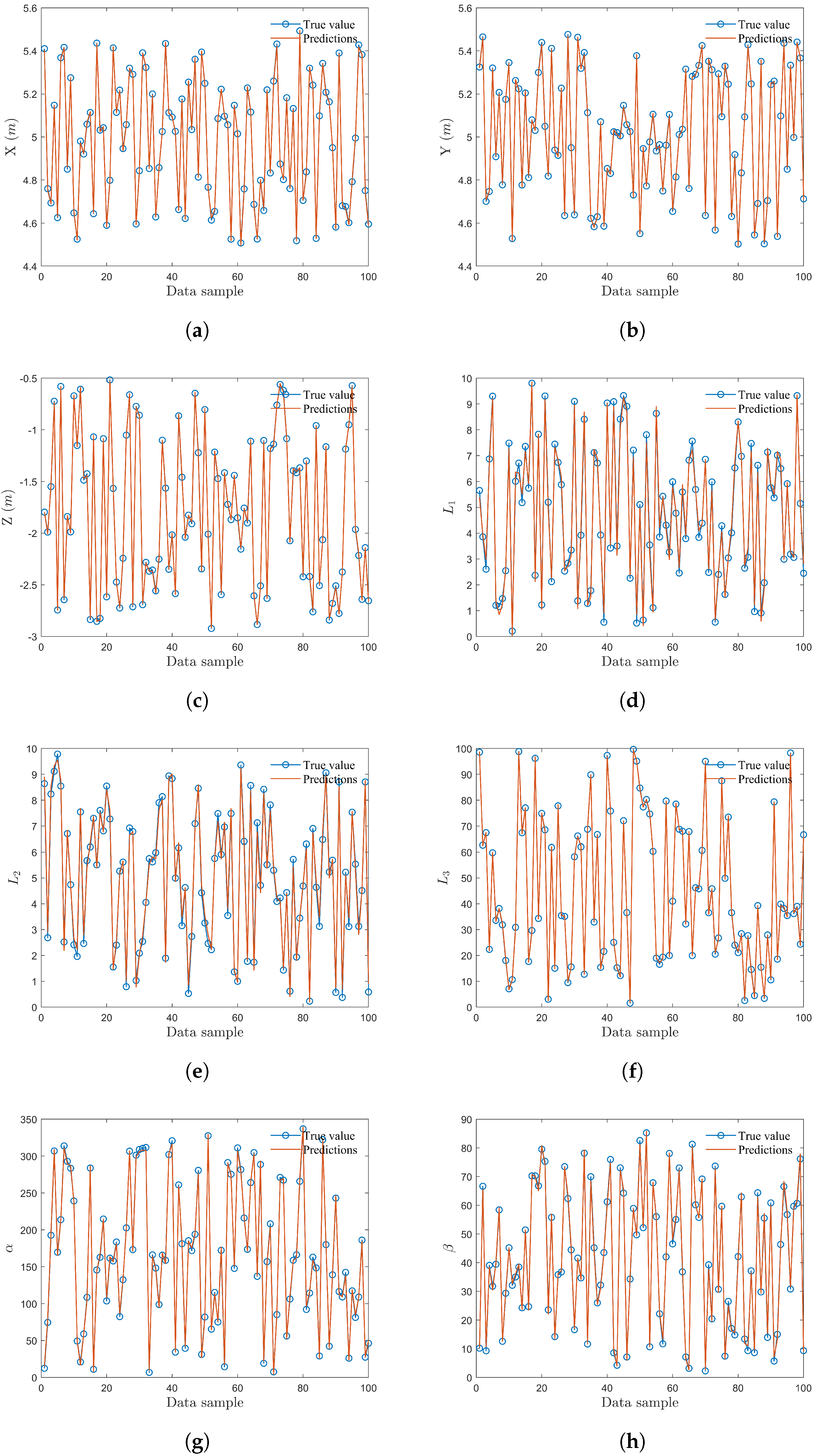
To further assess the effectiveness of MagEMNet, we randomly selected 100 samples from the test set for additional predictions. The predicted values were then compared with the true values, as depicted in Figure 8.

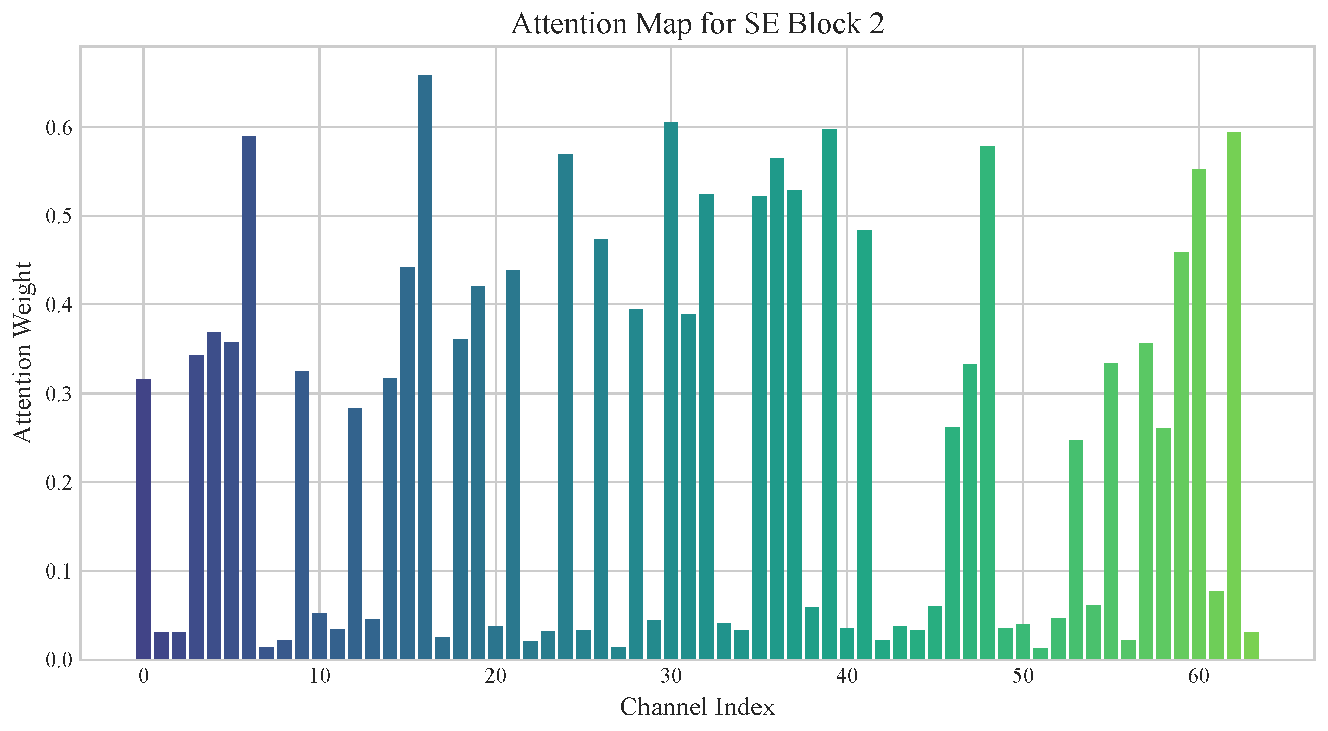
The attention weights for SE Block 1 are illustrated in Figure 9. The focus is concentrated on specific channels with high weights. The attention weights for SE Block 2 are displayed in Figure 10. This block demonstrates a more even distribution of attention across multiple channels.

For spatial parameters, the model showed high consistency between the predicted and true values of the target’s position coordinates x, y, and z. The dipole moment $L_3$ exhibited slightly lower accuracy due to its larger magnitude, which introduces greater variability in predictions. Conversely, the parameters $L_1$ and $L_2$, with lower magnitudes, were more susceptible to the influence of $L_3$, resulting in minor deviations for a few samples. Overall, the deviations were minimal and did not significantly impact the prediction quality.

Moreover, MagEMNet achieved strong accuracy in predicting the rotational angle $\alpha$ and inclination angle $\beta$, with no substantial discrepancies noted across the sample set. These findings validate the efficacy of MagEMNet in accurately inverting target parameters, confirming its robustness and suitability for subsurface exploration applications.

We systematically evaluated the performance of our proposed MagEMNet inversion model by conducting comparative analyses with several established inversion methods, include DNN [7], LM [36], and BAD [37]. This evaluation includes both qualitative and quantitative assessments to highlight MagEMNet’s efficacy in accurately resolving subsurface parameters.

Table 3. Quality assessment metrics comparison on our dataset.

Method	Coefficient of Determination (${\mathit{R}}^2$)	Explained Variance (EV)	MSE	MAE
DNN	0.853	0.824	1.152	0.552
LM	0.658	0.634	1.562	0.854
BAD	0.781	0.755	1.359	0.635
Ours	0.929	0.927	0.956	0.483

The best results are highlighted in bold in the table.

presents the experimental results obtained using these methods on our dataset. For quantitative analysis and comparison, we calculated response estimation outcomes based on the specified metrics. As shown in Table 3, our method consistently outperformed others in terms of quantitative performance.

5.3.2. Field Experiments

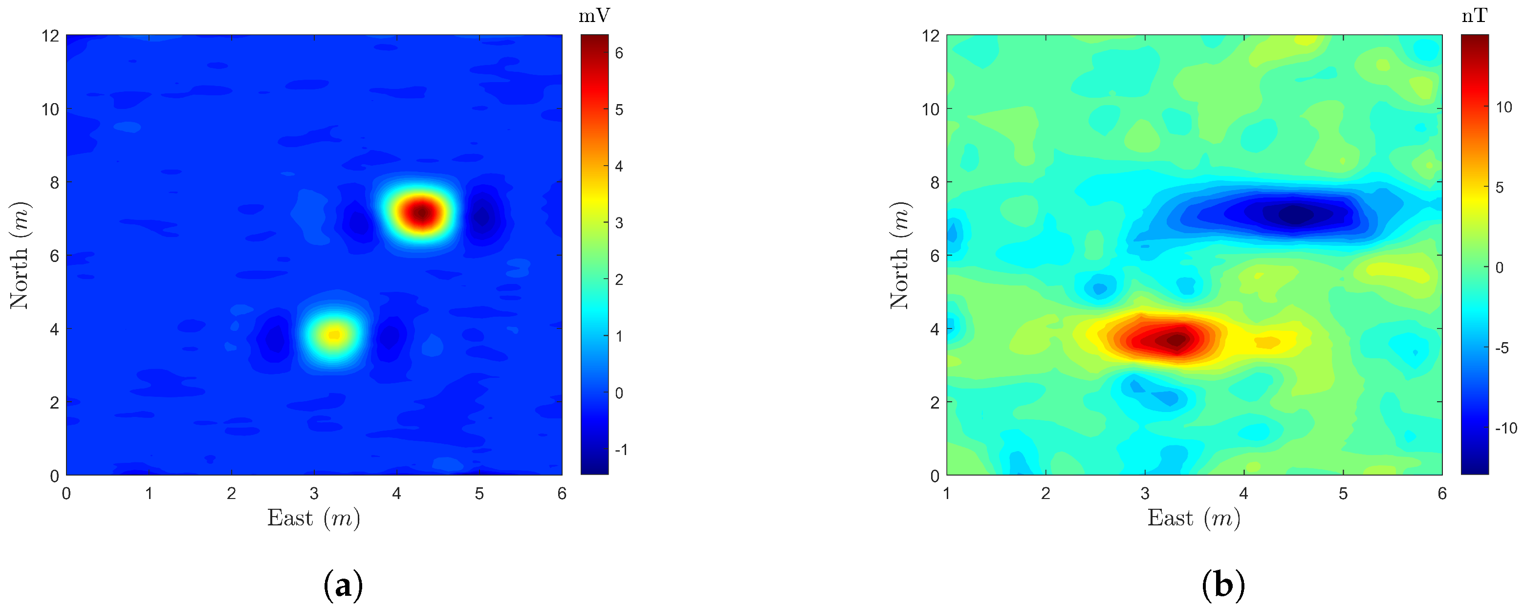
The experimental site was located in Huayin City, Shaanxi Province, where the integrated exploration system was systematically assessed for performance. A 7 m × 10 m test area was designated, characterized by a lack of vegetative cover and a series of terrain undulations with vertical variations of approximately 30 cm. A joint experiment was conducted employing the laboratory-developed UAV-borne magnetic detection system (UAV-MAG) in combination with an integrated UAV-based time-domain electromagnetic detection system (UAV-TDEM). Within the test area, two steel targets were precisely positioned at coordinates (4.49, 7.19, −0.80) and (3.32, 3.76, −0.40), with respective dimensions of $\mathrm{\Phi }8\times 28$ cm and $\mathrm{\Phi }6\times 18.5$ cm.

Figure 11 illustrates the electromagnetic and magnetic responses within the survey area, clearly highlighting the responses of the two targets. The vertical axis represents the northward position, meaning the top of the figure corresponds to the northernmost area in the survey. The horizontal axis represents the eastward position, ensuring a conventional north-up orientation as commonly used in maps. In the electromagnetic response, only the Z-component was collected, resulting in exclusively positive values. Due to the rapid attenuation of the electromagnetic response, the anomaly regions are relatively compact. In contrast, the magnetic response exhibits both positive and negative anomalies, attributed to the relative orientation between the targets and the geomagnetic field.

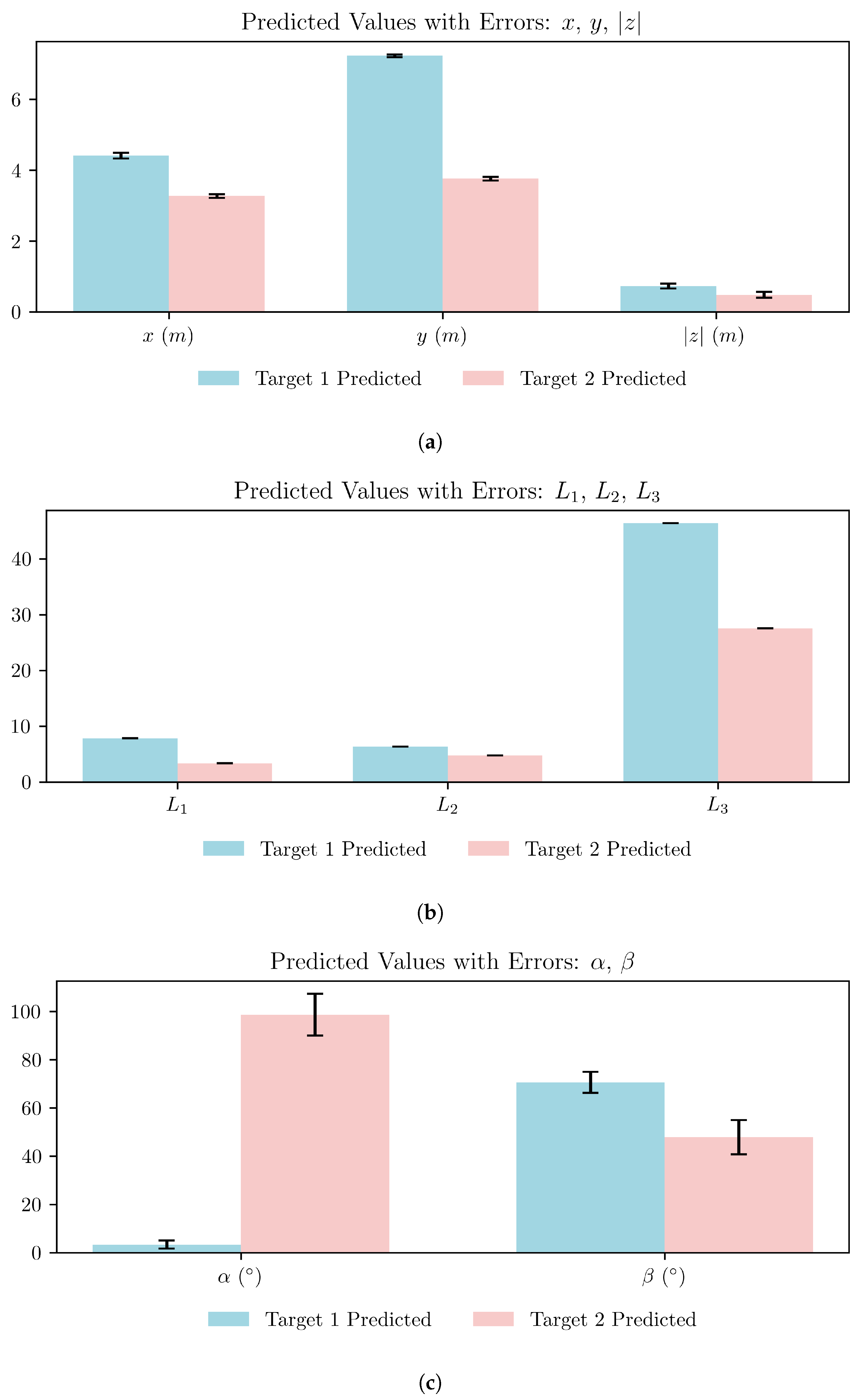
Given that our simulation region spans the range $[3.5,6.5]$, we initially rescaled the area to ensure alignment with the defined simulation boundaries. Subsequently, two sets of data were input into MagEMNet for inversion, with the results presented in

Table 4. Inversion results of measured sample.

Sample 1	Target 1	MagEMNet	Target 2	MagEMNet
x (m)	4.49	4.41	3.32	3.27
y (m)	7.19	7.23	3.71	3.76
z (m)	−0.80	−0.73	−0.40	−0.48
$L_1$	-	7.84	-	3.36
$L_2$	-	6.35	-	4.75
$L_3$	-	46.37	-	27.53
$\alpha {(}^{\circ })$	5.00	3.36	90.00	98.64
$\beta {(}^{\circ })$	75.00	70.63	55.00	47.89
Time (s)	-	0.0012	-	0.0009

. Figure 12 shows the predicted values for two targets with corresponding error bars. The visualization highlights the differences between the predicted parameters for both targets, including spatial and angular metrics.

The inferred coordinates of the two target locations closely approximate the actual values, with depth errors within 10 cm. Target 1, having relatively larger dimensions, resulted in a higher $L_3$ value compared to Target 2. Additionally, both targets exhibit symmetry, as indicated by the similarity between the inverted $L_1$ and $L_2$ values. These findings confirm the proposed method’s high accuracy and robust generalization capability.

6. Conclusions and Future Work

This study introduced MagEMNet, a novel convolutional neural network (CNN)-based framework tailored for the joint inversion of electromagnetic (EM) and magnetic data. Addressing the inherent limitations of traditional single-modality geophysical inversion methods, MagEMNet effectively integrates the complementary strengths of EM and magnetic field responses, enabling precise and robust subsurface exploration while maintaining computational efficiency. The model’s architecture incorporates advanced deep learning features, including Squeeze-and-Excitation (SE) blocks and a physics-constrained loss function, enhancing its capacity to capture complex spatial relationships and adhere to the underlying physical principles governing geophysical processes.

The synthetic dataset generation and forward modeling processes were meticulously designed using a unified three-dimensional orthogonal magnetic dipole model. This ensured a consistent representation of subsurface properties, providing a strong foundation for model training. The effectiveness of MagEMNet was validated through comprehensive synthetic and field experiments, demonstrating its superior performance in accurately predicting key target parameters such as spatial position, dipole orientation, and magnetic polarizabilities. Quantitative assessments confirmed high predictive accuracy, with a coefficient of determination ($R^2$) exceeding 0.92 and significantly reduced error metrics compared to traditional methods like DNN, LM, and BAD. Field experiments further validated the model’s practical applicability, showing its ability to resolve target parameters with depth errors of less than 10 cm and delineate target characteristics with remarkable precision.

MagEMNet also showcases the capability of deep learning to overcome the non-uniqueness problem prevalent in traditional inversion methods. Unlike conventional techniques, which often require extensive prior knowledge and are susceptible to local minima, MagEMNet leverages data-driven training to achieve superior inversion results. Moreover, the introduction of a physics-constrained loss function imbues the model with physical interpretability, enhancing its robustness and preventing over-reliance on data-driven learning alone. These advancements underscore the framework’s potential to address the challenges posed by the complexity and heterogeneity of subsurface targets.

While MagEMNet demonstrates significant advancements in joint inversion of electromagnetic (EM) and magnetic data, several challenges remain that need to be addressed to enhance its applicability in more complex and diverse geological scenarios. These challenges and the corresponding proposed solutions are outlined below.

(1) Data Complexity and Dataset Size: The performance of MagEMNet is highly dependent on the quality and representativeness of the training datasets. For larger or geologically complex datasets, capturing the required diversity to model subsurface heterogeneities can be a considerable challenge. To address this, future research will focus on generating synthetic datasets using advanced forward modeling techniques capable of simulating complex geological features and various noise levels. Additionally, collaborations with research institutions to collect diverse real-world datasets will be pursued to ensure broader generalization.

(2) Computational Resource Requirements: The processing and training of large-scale three-dimensional (3D) datasets significantly increase memory and computational demands. This limitation is particularly critical for real-time applications and high-resolution data inversion tasks. To overcome this, we propose adopting strategies such as distributed training, model parallelization, and computationally efficient architectures (e.g., lightweight CNN variants or transformer-based models). These optimizations aim to reduce computational costs while maintaining or improving model accuracy.

(3) Geological Assumptions and Complexity: The training data utilized in this study assume relatively homogeneous and isotropic geological conditions. Such simplifications may not adequately represent heterogeneous or anisotropic subsurface environments, which are common in real-world settings. Future iterations of MagEMNet will integrate physics-informed priors and more sophisticated geological models to better capture these complexities. This will enhance the physical realism of training data and improve the reliability of inversion results.

(4) Model Interpretability and Generalization: As MagEMNet is scaled to include more diverse datasets and geological conditions, maintaining model interpretability and avoiding overfitting become critical challenges. To address these issues, we plan to incorporate regularization techniques and domain adaptation methods to improve generalization. Additionally, attention-based explainability modules will be explored to provide insights into the decision-making process of the model, thereby enhancing its interpretability for practical applications.

By addressing these challenges, MagEMNet can further evolve into a robust and versatile tool for joint geophysical inversion across a wider range of geological environments. These future directions will not only improve its computational efficiency and generalization capabilities but also extend its applicability to more complex and heterogeneous geological contexts, contributing to the broader field of geophysical exploration.

The practical implications of MagEMNet are broad, spanning applications such as unexploded ordnance detection, subsurface resource exploration, and environmental monitoring. Its ability to detect both ferromagnetic and non-ferromagnetic metal targets, as well as derive accurate position, shape, and orientation information with sub-decimeter accuracy, confirms its versatility in field applications. Furthermore, the negligible prediction time required for subsurface anomaly characterization makes MagEMNet a viable tool for real-time exploration tasks.

Future research directions include enhancing the generalization capabilities of MagEMNet by incorporating multi-scale data integration and domain adaptation techniques. Additionally, expanding the framework to include other geophysical modalities, such as gravity and seismic data, will enable a more comprehensive understanding of subsurface environments. Leveraging such multimodal approaches could further reduce solution ambiguity and improve the reliability of inversion results in complex geological settings.

In summary, MagEMNet represents a significant step forward in geophysical inversion, offering a robust, efficient, and scalable solution for subsurface exploration. Its integration of advanced machine learning techniques with geophysical principles provides a powerful framework for addressing the challenges of subsurface characterization in diverse geological scenarios.