Design and Calibration of a Sensory System of an Adaptive Gripper

Abstract

The design and calibration of an adaptive gripper’s sensor system are presented in this research. Including the final constructive variants, the variants of the planned force sensor and slip sensors are detailed, highlighting their primary functional and constructive features. The key elements regarding the calibration of the force and slip sensors on each gripper module of the adaptive gripper are then displayed. Each sensor must be examined and calibrated independently due to its construction particularities. The important force and slip sensor behavior graphs are displayed, along with the calibration needed to ensure the adaptive gripper operates as intended. This paper suggestively shows, among the few papers of this kind, for the first time, the laborious but absolutely necessary process of calibrating force and slip sensors for gripping in general, and for adaptive gripping in particular.

1. Introduction

Adaptive grippers are gripping systems used in industrial robots to grip parts of various shapes and sizes. Also, in many cases, it is more efficient to design a gripper adapted to a series of real robotic applications, for gripping parts of varied shapes and with relatively large variations in size. In addition, adaptive gripper systems are able to take into account the particularities of the gripped part (shape and weight) and make decisions to obtain a safe grip, thanks to the provision of appropriate sensory systems. As examples of such grippers, three cases are first presented: Robotiq 2 Finger Adaptive [1], with a single contact area with the gripped object on each holder element; the SamPlIng gripper [2], which has two contact areas with the gripped object on the holder elements, and the evaluation of dynamic adaptation for a sinusoidal test signal is presented without details about the calibration of the sensors used; the Cassino 1 gripper [3], which uses piezoelectric force sensors, without detailing the calibration stage; and the Cassino2-LARM Hand gripper [4], which has a higher degree of adaptation to the type of gripped part. An adaptive gripper with three jaws that can be replaced by three fingers is described in [5], with the possibility of two fingers adapting to the orientation of the surface of the piece to be gripped by self-orientation. A gripper similar to the Barrett gripper is described in [6], which can grip small parts especially by grasping, without referring to the calibration of the sensors used. In the paper [7], a gripper with local adaptivity, with two fingers, specialized for gripping and manipulating, including the mounting of electronic cables, is described without referring to the sensors used. Another somewhat adaptive gripper capable of gripping parts at predetermined points is described in [8], which shows the use of depth sensors, without detailed references to them. These grippers tend to be used more and more to replace grippers with jaws [9], which are limited to gripping a single type of shape or size. In the papers [10,11], which focus on the calibration of sensors used in robotic gripping systems, specifically a force sensor and a slip sensor, different situations are analyzed than the one in this work and at a much more general level. The information in this regard is limited, and the complexity of the calibration process is not adequately highlighted, which is what the present paper aims to address. This paper briefly presents the design, highlighting the innovative aspects, and in more detail the calibration of the force sensor and the slip sensor for each gripper module. This paper first presents the logical architecture for the design of the electro-electronic part of each gripping module. It then describes the main elements of the design of the slip sensor and the force sensor on each gripping module, after which the calibration of the force sensor and the slip sensor and the results of the validation tests of their proper functioning are presented. At the end of this paper, the gripping of two real parts with the designed adaptive gripping system is described, which validates the correct functioning of the designed and calibrated sensors used.

2. Materials and Methods

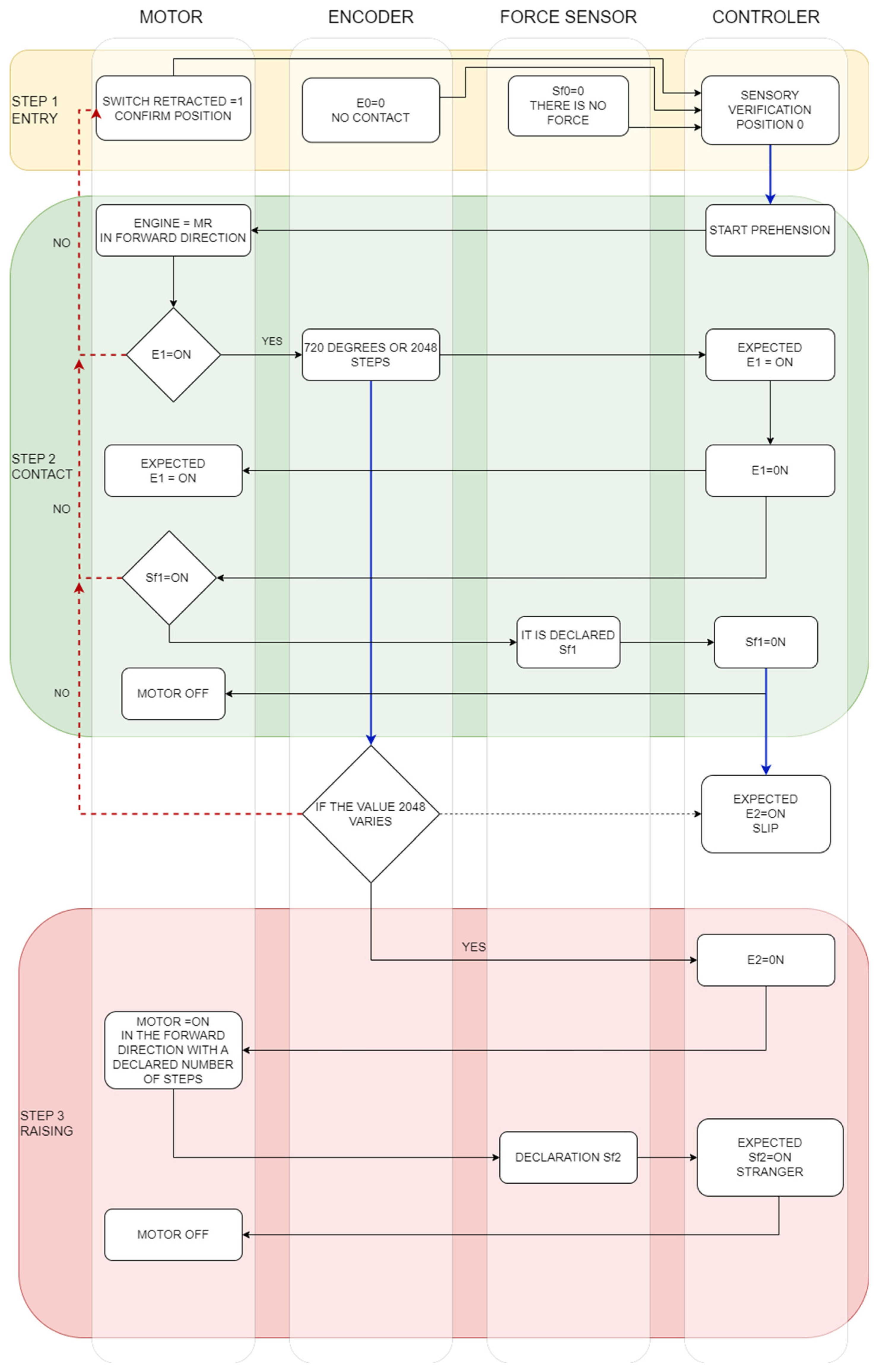
2.1. Logical Architecture of the Sensory System to Achieve Self-Adaptation

The logical architecture (Figure 1) for each gripping module is designed to perform gripping independently from a mechanical, electrical, and software perspective. Self-adaptive gripping is achieved in 3 steps:

Step 1—The sensor states are declared in the retracted position of the grasping module. If the module is in the forward position or in another intermediate position, then the controller makes the decision to reach the forward position and waits for the command to perform a new grasp.

Step 2—The module advance command has been received, and the sensory system is in the “ON” state permanently waiting for the collection of new states. This stage can be completed if the sensory system has fulfilled its software condition; namely, the module jaw has come into contact with the object to be grasped. After entering into contact, the clamping is performed until the force declared in the software is reached. The object does not move after the clamping has been performed.

Step 3—After step 2 has been completed, the sensory system detects that condition “3” in step 2 has not been met, which means that the slipping of the grasped object has been detected, and it enters the withdrawal phase. If, after the subsequent tightening, the sensory system detects movement, the tightening will be performed again; this will be repeated until the sensory system reaches the maximum declared thresholds, namely, the following:

-

The force has exceeded the maximum limits;

-

The slip has reached its maximum point.

When one of the maximum limits, among the above conditions, is reached, then the module will stop gripping.

According to the above logical architecture, the necessary steps were taken to design the slip sensor and force sensor on each gripping module and then to calibrate them, after which testing was carried out in real gripping situations with the designed and physically realized adaptive gripping; the details are presented below.

2.2. Sensory System Design

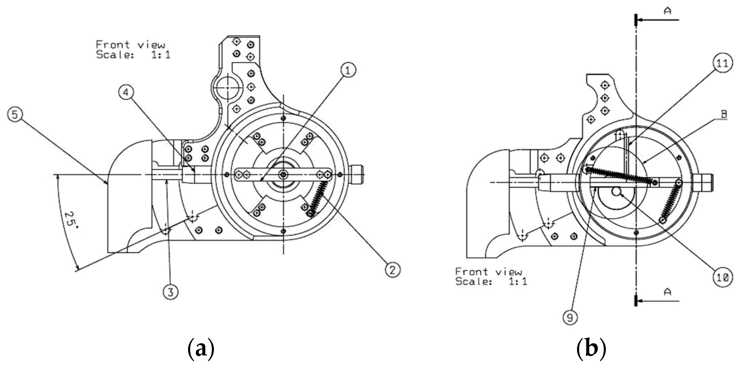
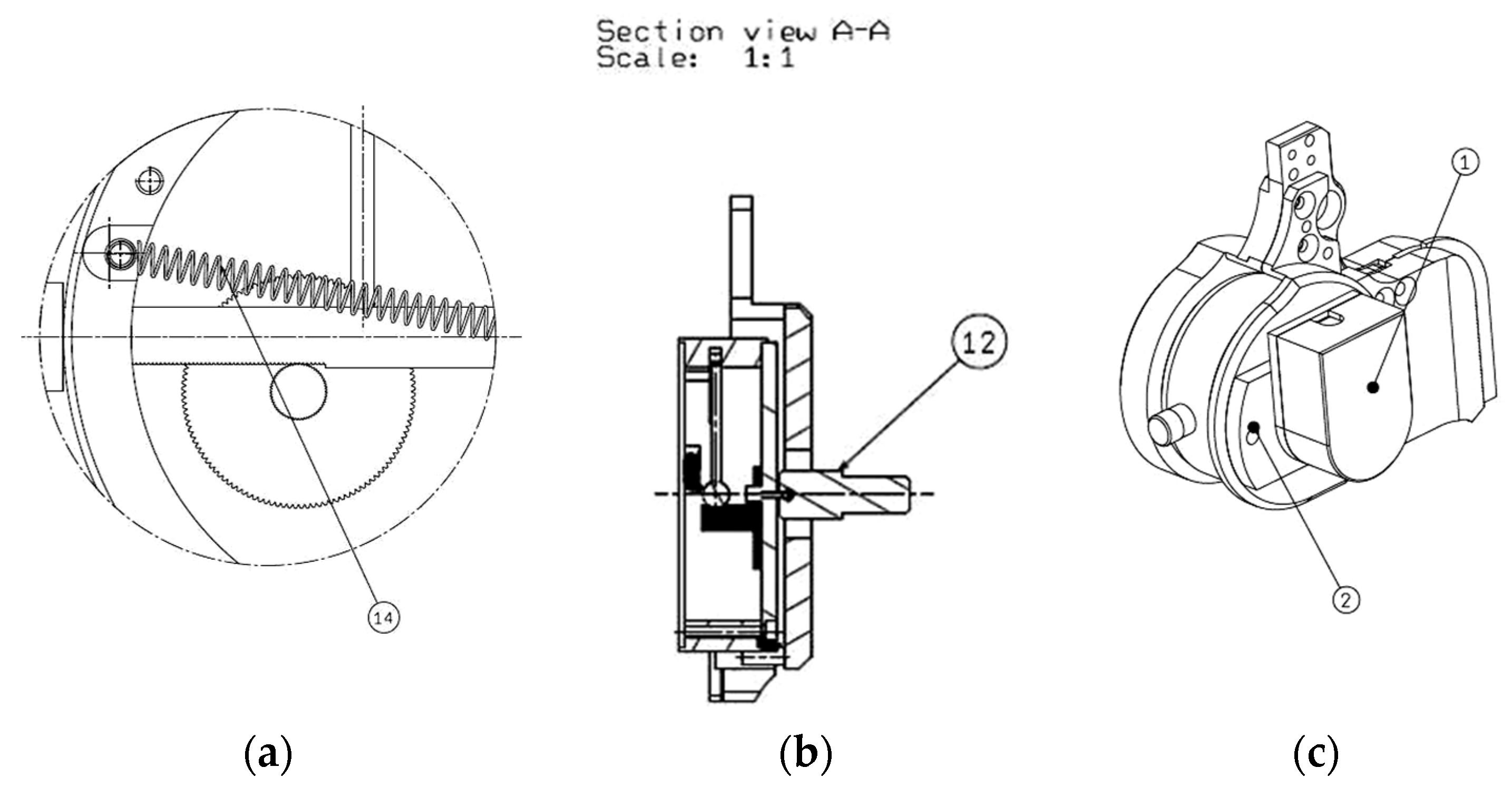
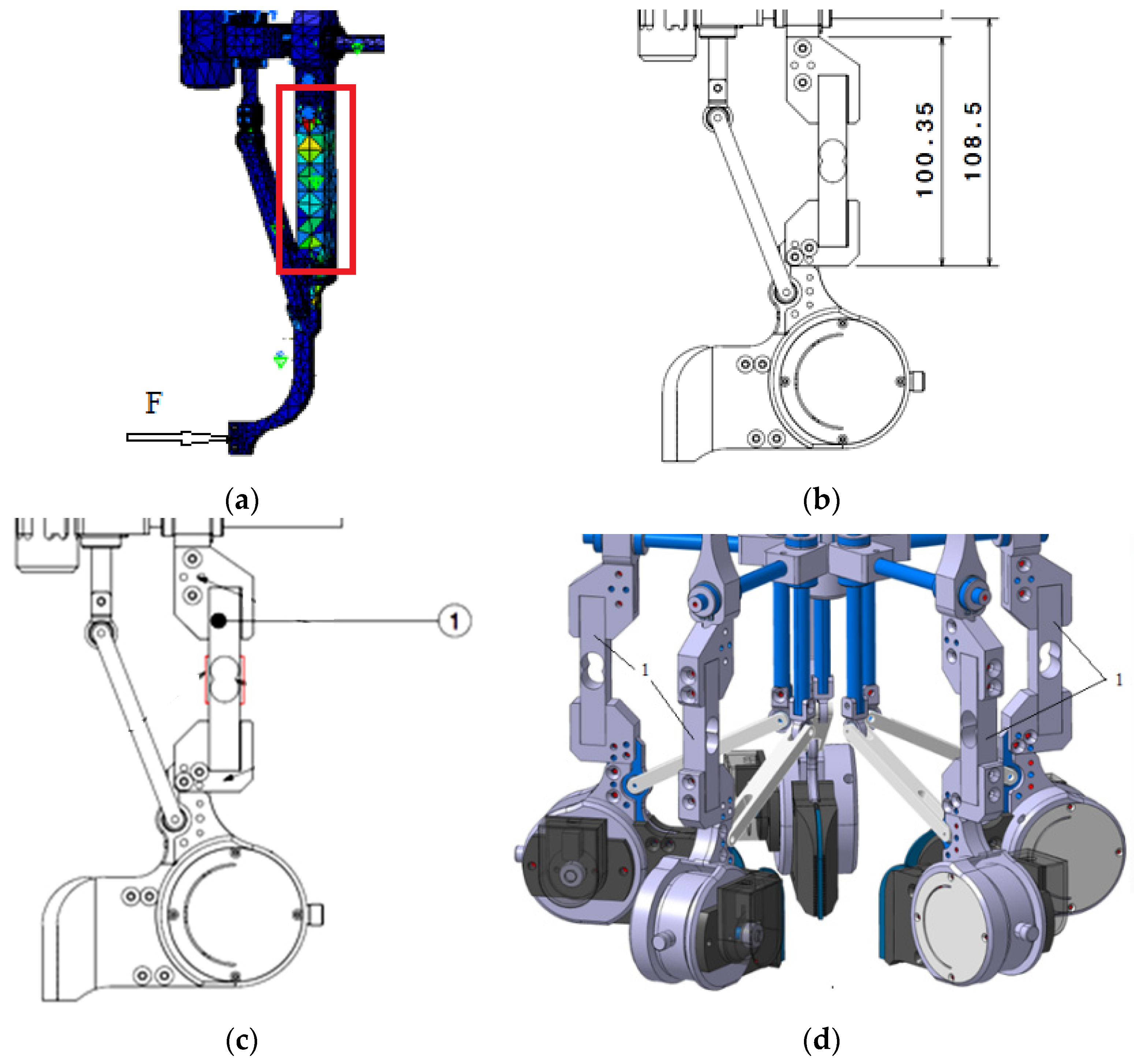
2.2.1. Slip Sensor Design

The self-adaptive gripper described requires a slip detection system to ensure safe and efficient gripping, especially for objects with irregular shapes and variable sizes. To this end, each of the five modules is equipped with a specialized slip sensor, designed to accurately measure the relative movements between the gripper and the manipulated object, without influencing the contact between them. Unlike existing solutions, the described sensor is optimized for gripping objects with small and medium thicknesses, commonly found in the automotive industry. In order to increase the gripping power and prevent the component from slipping and maintain the hold, the slip sensor’s job is to detect the part being gripped and send the appropriate signal if a slip is detected [12]. There are different architectures for slip sensors, including those presented in [13,14]. In this case, a variation with improved performance for the particular grip scenarios under consideration—namely, the grip of components with small and medium thicknesses and different shapes from the composition of subassemblies in vehicle construction—was achieved by designing the slip sensor.

As a result, the designed sensor must be able to measure slip without influencing the contact of the grasped object with the sensor jaws. To achieve this objective, the following are required:

-

The detection system for determining the slip of the object must be capable of performing simultaneous translational and rotational movements.

-

For the accuracy and sensitivity of the slip determination, an incremental optical encoder with a resolution of 1024 must be used.

-

The mechanism must not generate negative forces on the slippage measurement system.

-

It must be integrated dimensionally into the entire grasping module.

-

It must respect the kinematic structure of the grasping module from a dimensional point of view.

The sensor uses a mechanical design (Figure 2a,b), combining translational and rotational motions to detect slip. A flat strip (5), with a sticky surface, is placed in contact with the object. When the object begins to slip, the relative motion between the strip and the object triggers a rotational motion, amplified by a rack-and-pinion mechanism, which transmits the information to a high-resolution (1024) incremental optical encoder. The encoder converts the mechanical motion into digital data, signaling the slip. Thus, the sliding sensor system is based on the principle of detecting sliding by rotating around an axis an adherent system that comes into direct contact with the grasped object (Figure 2a) [15,16]. The component that comes into direct contact with the grasped object is a flat strip (5) that has an adherent surface in the contact area to ensure the transmission of movement. The flat strip is extended outside the jaws to make contact with the object by sliding the component (3), performing a translational movement by sliding through the component (4). The translational movement of the flat strip detects the contact with the object. The sensory system detects the sliding and detection of the object by transforming the movement of the R-T-R type (rotational movement into translational movement and from translation to rotation). Through this exchange of types of generated movements, the sensitivity of the movement increases [15]. After the gripping–approaching movement to the piece to be grasped is performed, the jaws are in contact with the object, and its movement can be performed. If it slides in the jaws, the flat band, from the translational movement it initially makes, performs a rotational movement with the entire translational system, moving component (1) at the same time. Component (1) is the part that ensures the return to position 0 of the sliding sensor with the help of the extension spring (2). The sliding sensor is equipped with an RGB LED that signals when the sensor is activated and when the sliding movement is performed by changing colors, and this can be observed through the slot (6) in Figure 2b.

With the aid of component (11) in Figure 2b, the sliding sensor that detects the grabbed object by translational movement guarantees its movement by preventing rotation. With a comprehensive illustration in Figure 3a, the rod that executes the translational movement has a toothing that resembles a rack and imprints the rotational movement on the gear wheel (10). Figure 3a provides a detailed view of the circled area in Figure 2b, highlighting the driving zone between the rack and pinion where the motion is amplified in terms of output rotations [17].

Rotation amplification is necessary because sensitivity in sliding is crucial. The translation system makes a stroke of 13 mm, and the rotation system makes 13 complete rotations, which means that at 1 mm, it rotates 360°. The sliding sensor’s movement is divided according to the translation stroke—namely, the object is gripped over 8 mm, with the rotation system rotating 280°; 5 mm of the stroke is left to compensate for the movement of the flat strip during sliding, where it performs both rotation and translation; to determine the sliding, a rotational movement of 25° is allowed. Following the translational movement, the entire system tensions an extension spring (14), which has the role of returning the mechanism to the forward position [15]. In the section of the sensory system in Figure 4b, it is highlighted that all movements made aim to generate rotations in component (12), which has the role of transmitting the final rotational movement to the encoder, which has the final role of determining the slip. In Figure 3c, an isometric representation of the designed slip sensor assembly is shown, where 1 is the encoder and 2 is the sensor body. Following the detailed design of all components, the CAD version was obtained (Figure 4a), respecting the dimensional integration conditions in the gripper module mechanism assembly. This led to the physical realization of the component parts and the slip sensor assembly shown in Figure 4b,c.

For the components of the slip sensor, we used the aluminum alloy AlCu4MgSi (alloy 2017 or similar), chosen for its high mechanical strength, lightness, good machinability, corrosion resistance, and relatively low cost. For the side parts that flank the jaws, we opted for black POM C (polyoxymethylene). The choice of this material is justified because it has high wear resistance, dimensional stability, impact resistance, and chemical compatibility with numerous lubricants and chemicals, which is important in the industrial environment.

The data from the encoder are processed by the controller of the respective module. If the sensor detects slippage, the controller automatically adjusts the gripping force to stabilize the object. The RGB LED provides visual feedback on the sensor’s status (active, slippage detected). The dimensional and kinematic integration of the sensor in the module is crucial for the optimal functioning of the entire system.

The designed sensor has the following important advantages:

• Precise detection of slip: the combination of translational and rotational movements, amplified by the rack-and-pinion mechanism, increases the sensitivity of the sensor;
• High resolution: the 1024-pulse incremental optical encoder ensures precise detection of even the smallest movements;
• Optimal integration: the compact design and kinematic compatibility allow for easy integration into the gripping module.

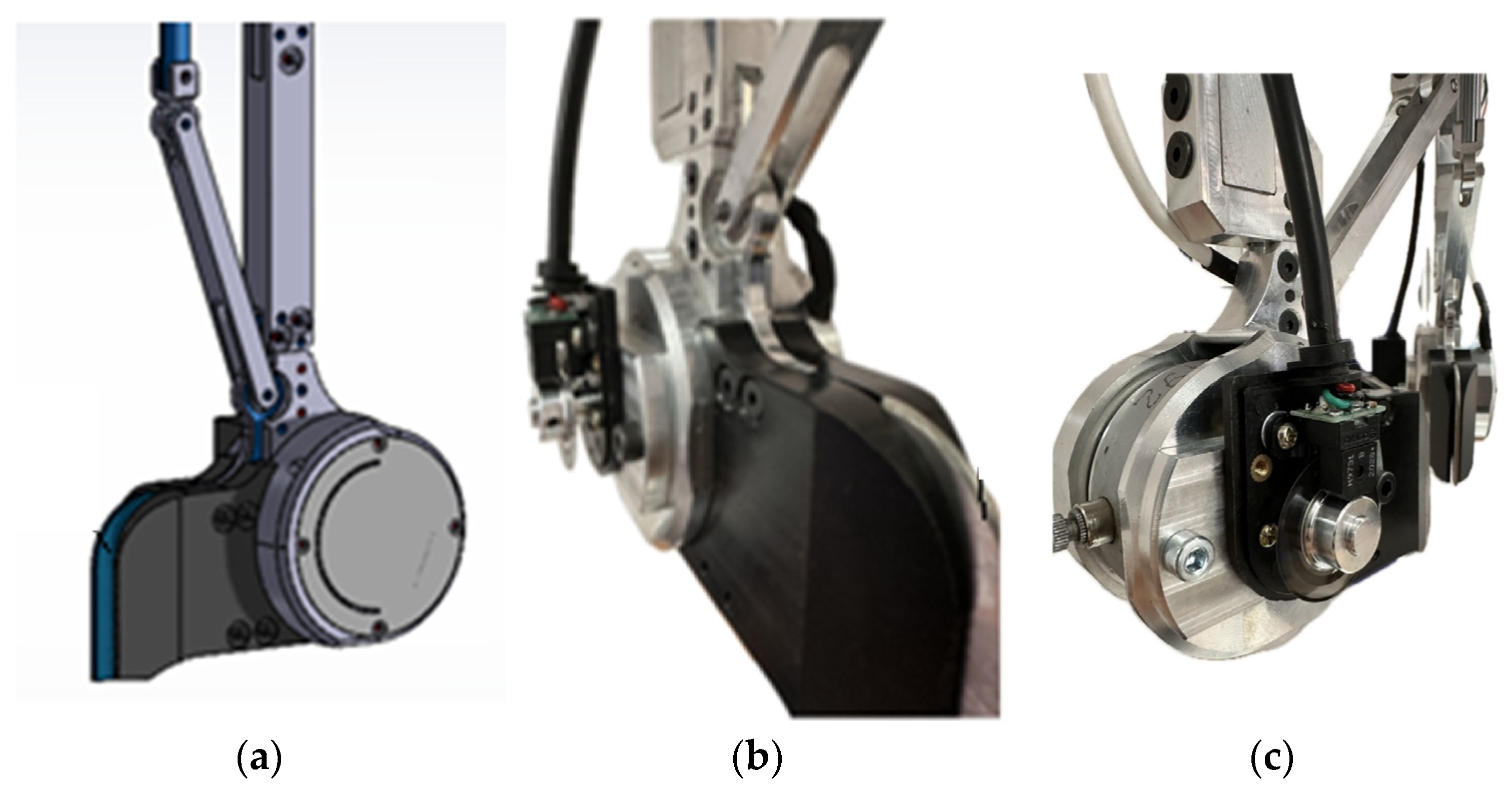
2.2.2. Force Sensor Design

The force sensor has the role of measuring the gripping force, in real time, up to the value necessary to grip a part, including adjusting this force to avoid the tendency of the part to slip in the gripper. In [18,19], systems for adapting the gripper configuration to the shape of the piece being gripped are described, supporting the adoption of the solution proposed in this paper. The force sensors in the equipment of some grippers, including adaptive grippers, are described in [20,21,22,23]. In this case, a Wheatstone bridge resistive force sensor was used, which was placed in the most appropriate part of the mechanical structure of the gripping module for maximum efficiency. For this, the material from which the components of the gripping module mechanism were made, namely duralumin, was first determined, and the gripping force applied to the gripping module jaw was established at a force of F = 1 kg. The MEF analysis of the mechanical structure of a gripping module was then used, and the area of maximum deformation was identified: the area framed in red in Figure 5a. The respective redesigned element is shown in Figure 5b, highlighting the size of the part of the element containing the force sensor. In Figure 5c, this part of the mechanism of the gripping module is shown, in which the notations represent the following: 1—the support piece of the force sensor, 2—the mounting parts in the mechanism element, 3—the Wheatstone half-bridge formed by two piezoresistive sensors, and 4—cutout to increase the sensitivity to deformation. Figure 5d shows the CAD shape of the force sensor area integrated into the respective element of the gripping module, with the parts marked with 1.

The use of a resistive Wheatstone bridge force sensor in this application offers several benefits over other types of force sensors, such as piezoelectric or capacitive ones, namely, the following:

Low cost: Resistive Wheatstone bridge sensors are generally cheaper than piezoelectric or capacitive sensors, which makes the solution more economical, especially in industrial applications where multiple sensor modules are required;

Robustness: Resistive sensors are generally more robust and more resistant to shock and vibration than piezoelectric sensors, which are more fragile. This is an important feature for a gripper operating in a demanding industrial environment;

Linearity: Resistive Wheatstone bridge sensors, properly calibrated, provide a fairly good linear relationship between the applied force and the output signal. This linearity simplifies signal processing and the implementation of control algorithms;

Simplicity: Integrating a resistive sensor into a circuit is relatively straightforward, requiring a simple signal amplifier (such as the HX711 used in this application). This reduces system complexity and overall cost.

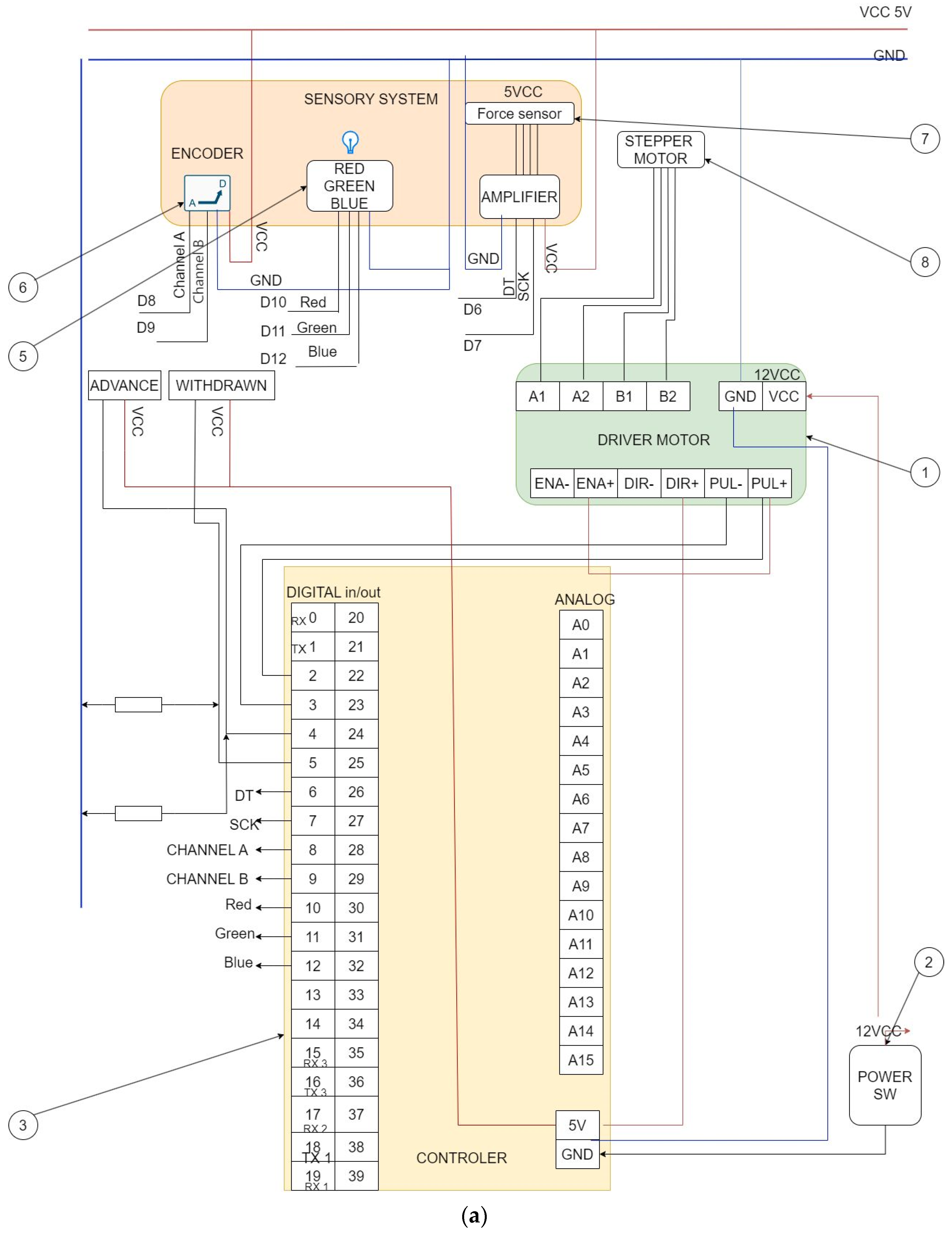
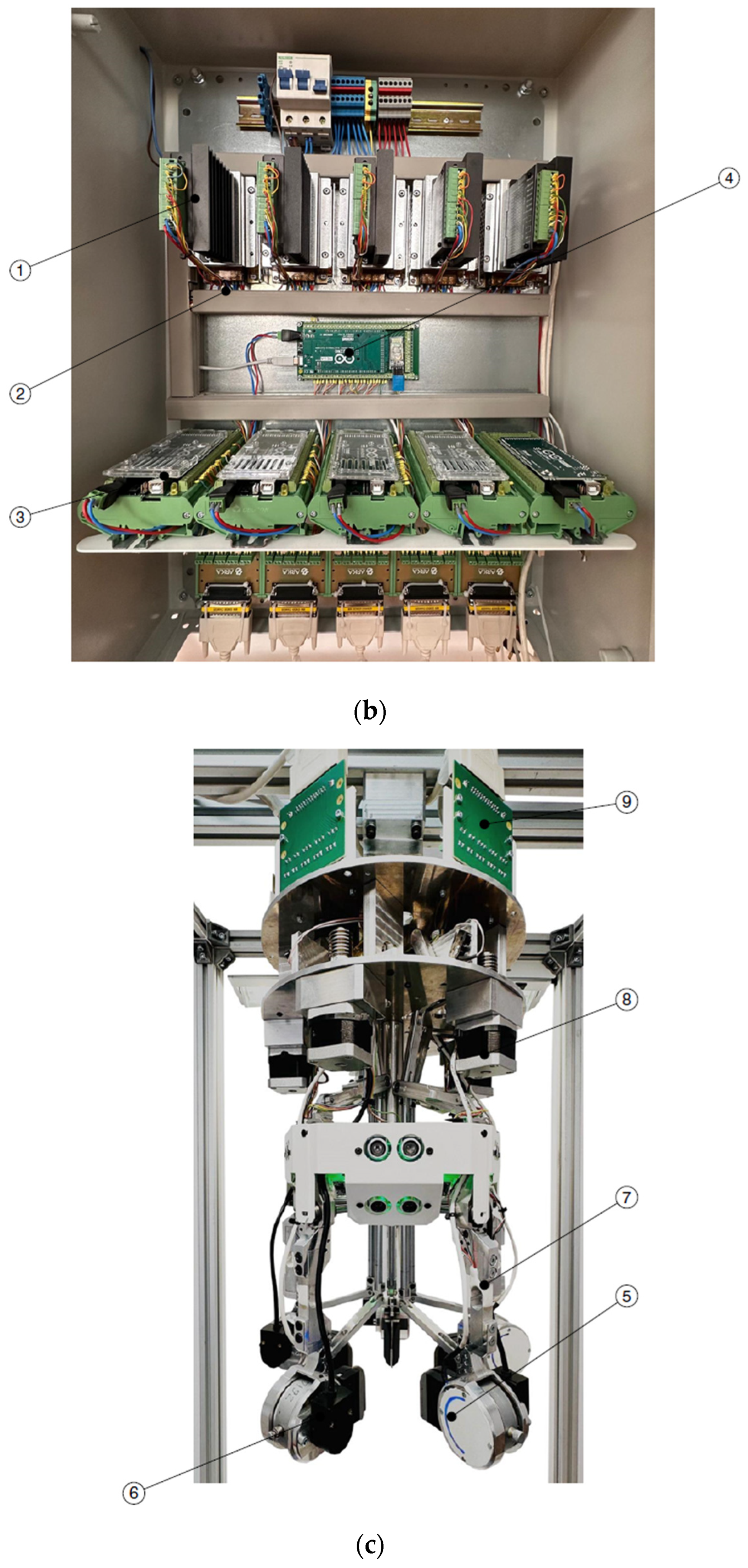
2.3. Design of the Electrical and Electronic Schematic of Each Gripping Module

For the design of the electrical scheme, the logical structure and all the electrical and electronic parts implemented on each module were taken into account. The important elements that were taken into account are as follows: the stepper motor with the programmable driver, the incremental optical encoder, the force sensor with the signal amplifier, the controller, and the stroke limitation contactors. The electrical and electronic scheme is shown in Figure 6a, the practically realized version in Figure 6b, and the real adaptive gripper in Figure 6c. The notations in Figure 6a are as follows: 1. Motor Driver Module 1, 2. Power Supply Module 1, 3. Controller Module 1 (Slave 1), 4. Master Controller (Figure 6b), 5. RGB LED, 6. Encoder, 7. Force Sensor, 8. Stepper Motor, and 9. Communication Module with Control Panel (Figure 6c). The electrical diagram (Figure 6a) illustrates a modular and distributed architecture, which reflects the mechanical design of the gripper. Each module (Slave I-V) has a dedicated controller (3), which locally manages the actuation of the stepper motor (8) via a driver (1). Each jaw’s movement can be precisely and independently controlled thanks to the incorporation of force sensors (7) and incremental optical encoders (6) in each module. To guarantee the best possible reading of the values, a signal amplifier is built into the force sensor circuit. The system is mechanically protected by travel limiters, which are the default in the diagram. Through a communication system (9), serial, or a communication bus, a main controller (Master, 4) oversees and manages the five Slave modules’ operations, enabling synchronized and adaptive gripper operation. Each module receives the required voltage from the power supply module (2). Each module’s state is visually shown by an RGB LED (5), which displays red for error, green for a successful grip, and blue for inactivity. The operation proceeds as follows: the Master controller receives commands from the user interface (not shown in the diagram) and transmits the instructions to the Slave controllers. The Slave controllers process the data from the sensors, control the stepper motor, and adjust the gripping force as needed. The two-way communication between the Master and Slave allows for adaptive, real-time control of the gripper.

The system maintains real-time responsiveness and accuracy through a combination of factors:

-

Hardware interrupts: The code uses hardware interrupts (attachInterrupt) to continuously monitor signals from the incremental encoder. This method ensures rapid detection of any change in probe position, without the need for constant checking in the main loop (loop()), which significantly improves response time.

-

Efficient slip detection algorithm: The slip detection algorithm (although simplified in the provided code) quickly analyzes variations in the probe’s angular position. Comparing consecutive encoder values allows for the rapid detection of unexpected movement, indicating slip.

-

PID controller: The PID controller quickly calculates the necessary adjustments to the clamping force based on data from the force and slip sensors. The derivative component of the PID controller is crucial for rapid response to sudden changes in position (slip). The PID function is implemented directly in the main loop, ensuring a continuous and real-time response.

-

High sampling rate: The code reads data from the sensors at a high enough frequency (10 Hz for the slip sensor, depending on how fast the loop() loop for the force sensor executes) to quickly detect any changes.

The integration of the sensor system with the overall adaptive grip control architecture is based on a distributed architecture, with a main controller (Master) and five secondary controllers (Slave), one for each module. Although the provided source code does not explicitly present a complete Master–Slave architecture, we can deduce the operating principle based on the available information:

-

Data acquisition from sensors: Each module (Slave) has its own set of sensors: a force sensor and a slip sensor (incremental encoder). The Slave controller collects data from these sensors locally, with a specified sampling frequency. The collected data are preprocessed locally (filtering, scaling) before being transmitted to the Master controller.

-

Communication with the Master controller: The Slave controllers transmit module status data to the Master controller via a digital communication channel using binary logic. This communication is bidirectional, allowing the Master controller to send commands to the Slave modules.

-

Master-level data processing and control: The Master controller receives data from all five modules. It processes these data to assess the overall condition of the gripper and the object being handled. The PID-based control algorithm makes decisions based on these data, adapting the gripping force and movements of each module.

-

Slave-level local control: The Slave controller receives commands from the Master controller and executes them locally. Using the PID algorithm, each Slave controller adjusts the gripping force and jaw movement to reach the setpoint set by the Master controller and to compensate for any detected slippage.

3. Results

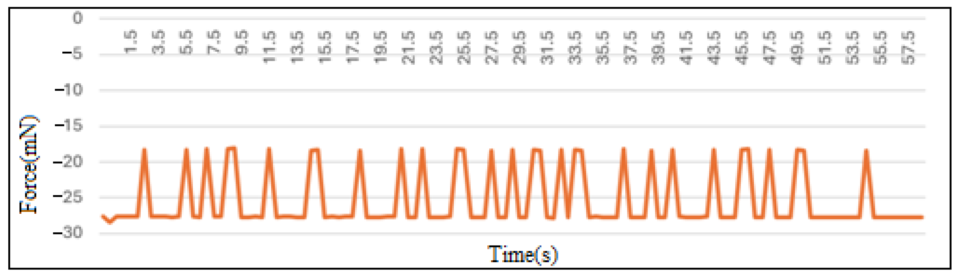
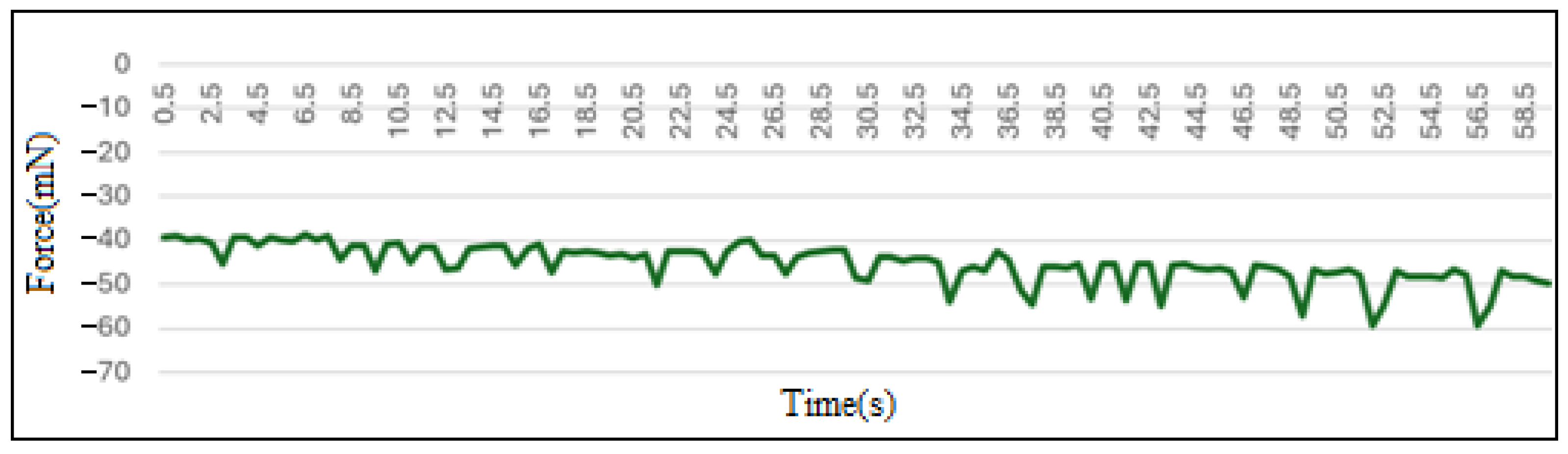
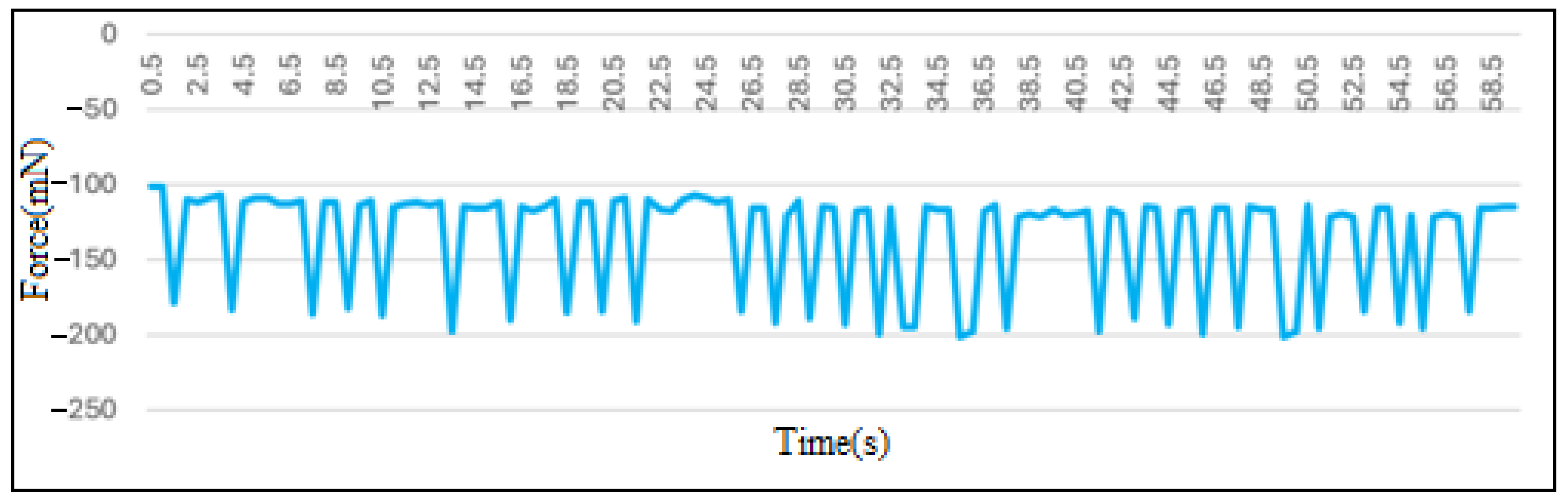
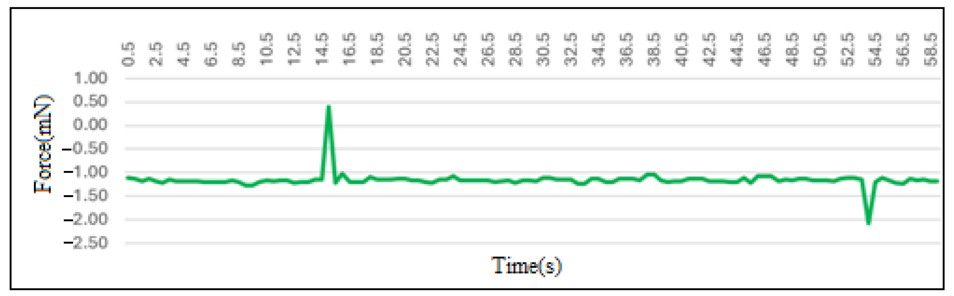
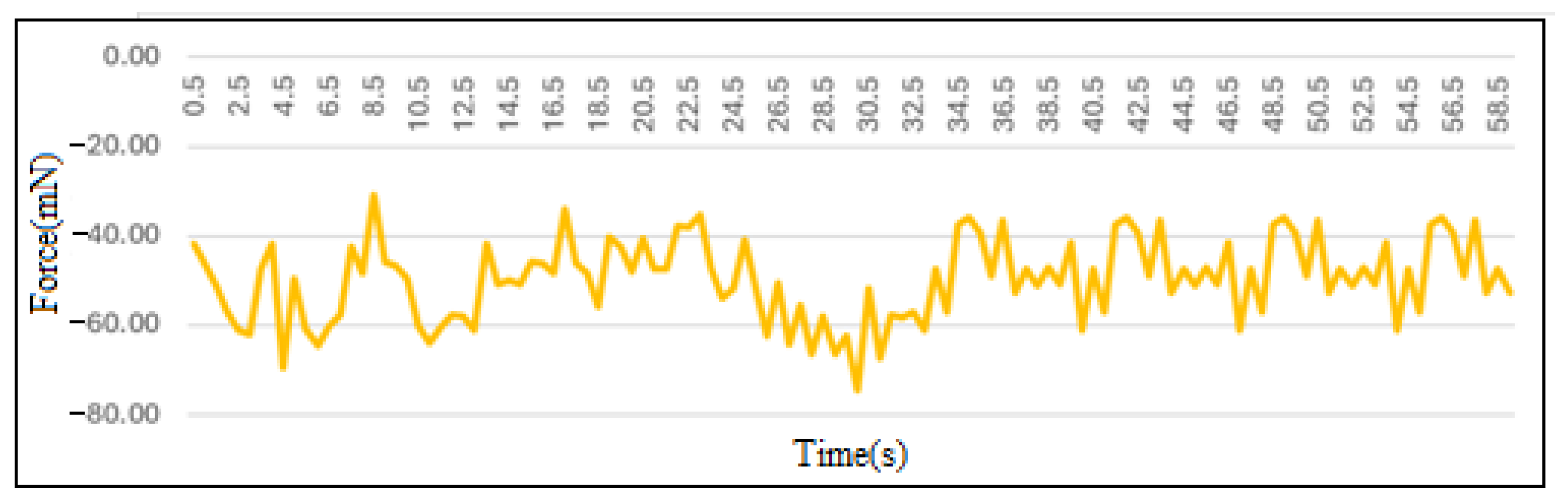
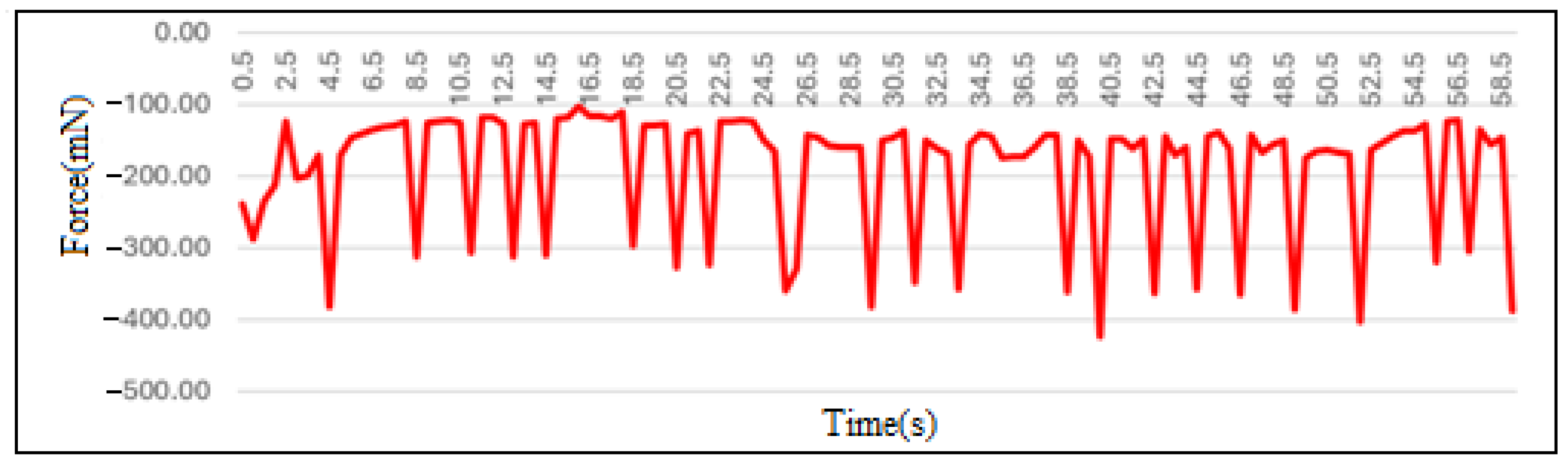
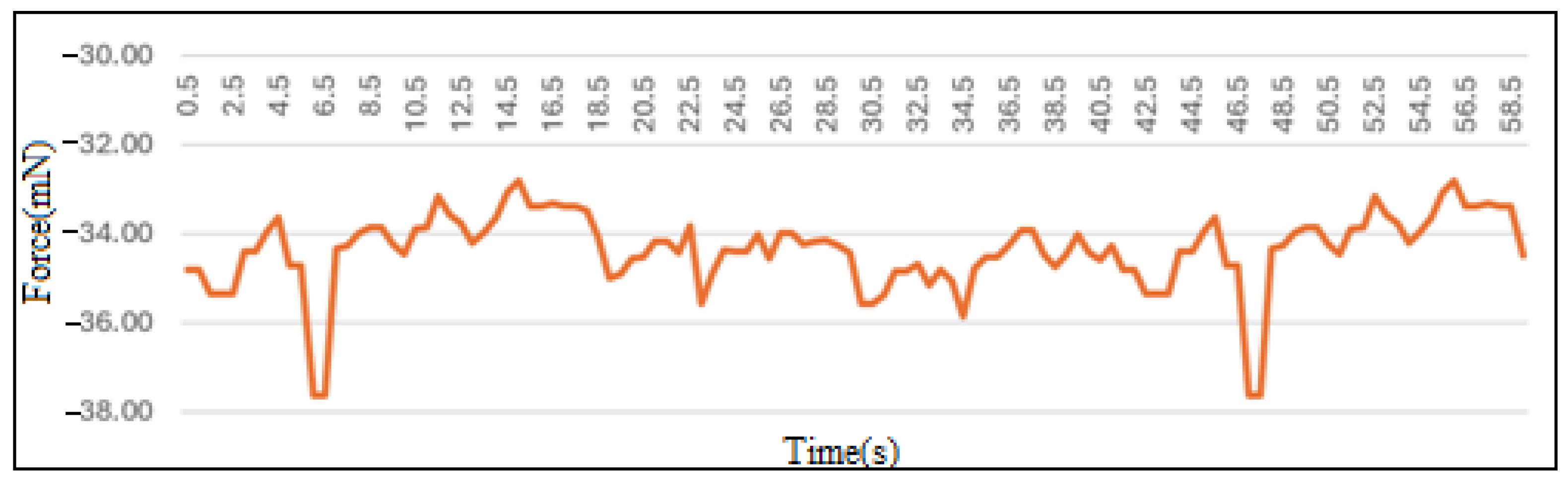
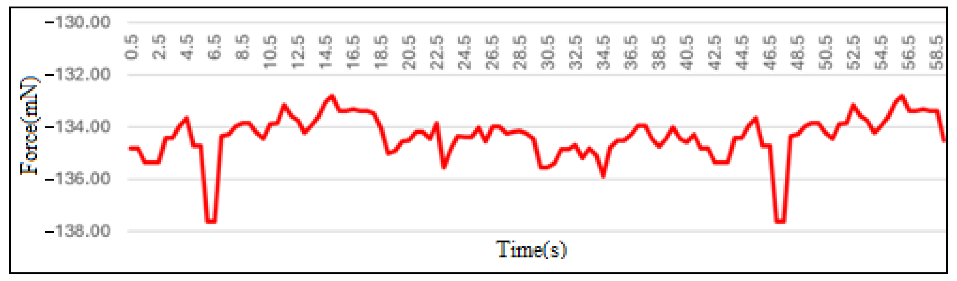
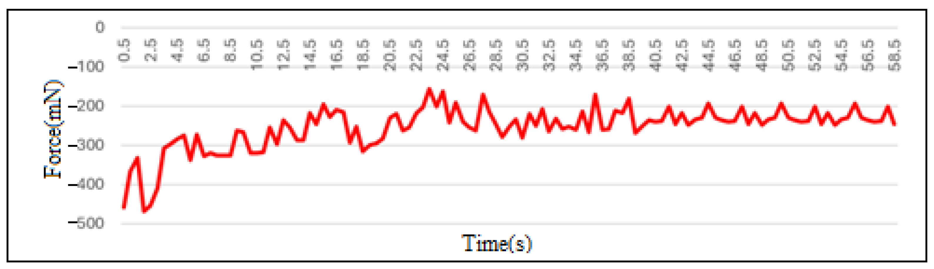
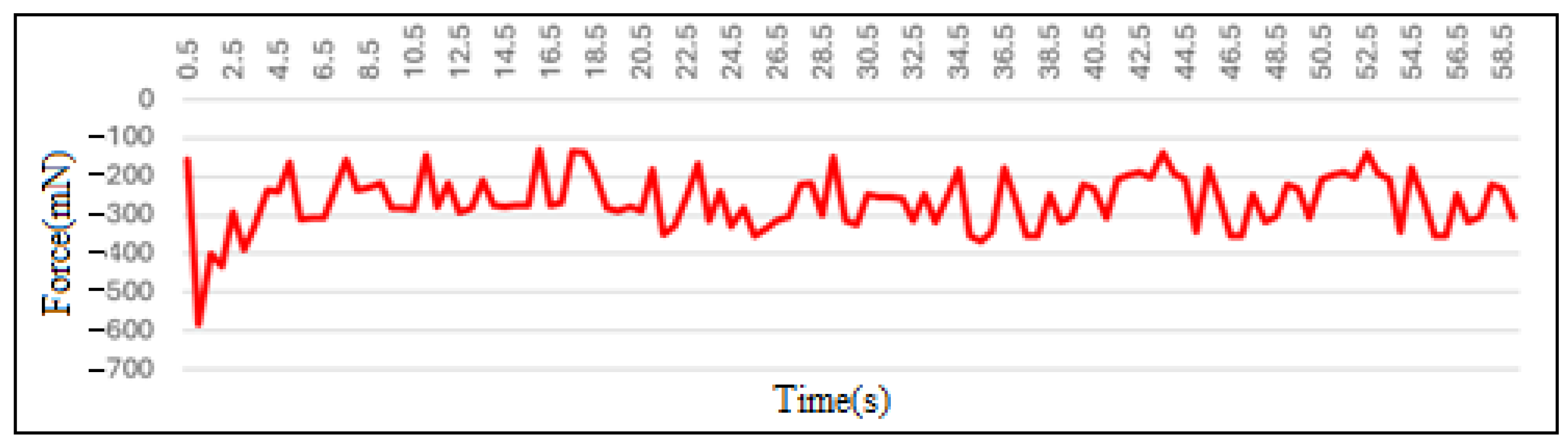
3.1. Calibrating the Force Sensor

Calibration of piezoelectric sensors, integrated in a Wheatstone half-bridge configuration (with two sensors per bridge), is essential for the accuracy of force measurements. The calibration process is performed in three phases:

-

Phase 1 (Quiet): The background noise of the sensors is measured, representing the voltage variations in the absence of any external force. This measurement is critical to determine the level of error inherent in the system and to establish a reference point for subsequent measurements.

-

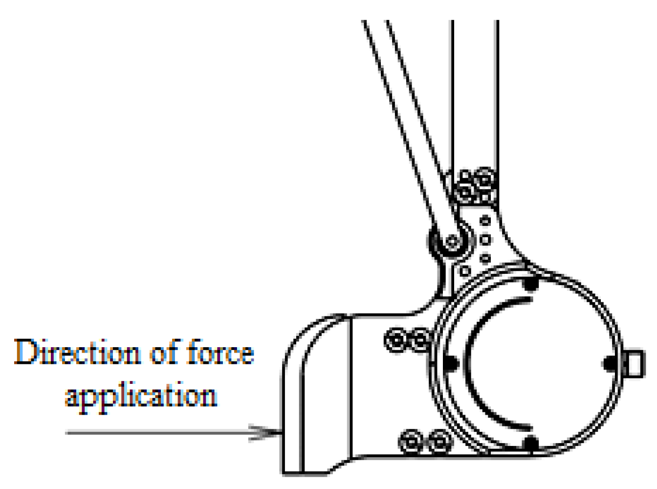
Phase 2 (Contact): A minimal force is applied, perpendicular to the force cell, simulating the initial contact with the object (Figure 7). The data collected allow the establishment of a threshold for detecting contact.

-

Phase 3 (Clamping): An increasing force is applied, perpendicular to the force cell, to calibrate the sensor’s response to force variations. This phase determines the direct relationship between the applied force and the value read by the sensor.

For data acquisition and calibration, we used an HX711 amplifier, connected to the ATmega controller via the SPI (Serial Peripheral Interface) interface. The developed software manages the SPI communication, the tare (resetting the sensor offset to zero), the scaling of the read values, and the weight display. A recalibration mechanism allows the sensor offset to be adjusted during operation, by sending a specific character (“t” or “T”) via the serial interface. The collected data (example in

Table 1. Collection of displayed data.

No.	Measurement Details
1	17:56:04.534 → Weight: −27.62 unity
2	17:56:05.045 → Weight: −18.34 unity
3	17:56:05.557 → Weight: −27.65 unity
4	17:56:06.115 → Weight: −27.66 unity
5	17:56:06.627 → Weight: −27.63 unity
6	17:56:07.182 → Weight: −27.74 unity
7	17:56:07.695 → Weight: −27.65 uniiy
8	17:56:08.209 → Weight: −18.25 unity
9	17:56:08.720 → Weight: −27.67 unity
10	17:56:09.279 → Weight: −27.68 unity
11	17:56:09.792 → Weight: −18.24 unity
12	17:56:10.305 → Weight: −27.65 unity
13	17:56:10.822 → Weight: −27.65 unity
14	17:56:11.376 → Weight: −18.15 unity
15	17:56:11.884 → Weight: −18.09 unity

) are subsequently processed and filtered to eliminate background noise and obtain precise calibrated values.

The steps of the software application and the meaning of the main code lines are as follows:

Step 1. The communication pins between the ATmega programmer and the HX711 amplifier were declared, in the form of constants:

“const int LOADCELL_DOUT_PIN = 6;”

“const int LOADCELL_SCK_PIN = 7;”

These lines declare two integer constants, LOADCELL_DOUT_PIN and LOADCELL_SCK_PIN, which represent the digital pins of the ATmega microcontroller used to communicate with the HX711 amplifier. The LOADCELL_DOUT_PIN pin is probably the amplifier’s data output pin, and LOADCELL_SCK_PIN is the clock pin. The choice of pins 6 and 7 is arbitrary and depends on the hardware configuration.

Step 2. The serial communication and its operating frequency were initialized:

“Serial.begin(9600);”

This line initializes the serial communication at a speed of 9600 baud. This communication is probably used to display calibration data on a serial monitor (e.g., a computer connected to the microcontroller).

“scale.begin(LOADCELL_DOUT_PIN, LOADCELL_SCK_PIN);”

This line initializes an HX711 scale, using the pins defined previously. It is assumed that scale is an object of a class that handles communication and reading data from the force sensor via the HX711 amplifier.

“ Serial.println(“Calibration…”)”

“Serial.println(“At this stage there should be no force applied to the sensor.”)”

“scale.tare();”

This line performs a “tare” of the scale, compensating for the sensor offset. This means that the sensor reading is set to 0 in the absence of force. This is an important step in calibrating the sensor to eliminate systematic errors.

“Serial.println(“Calibration completed!”)”

Step 3. Sensor calibration commands were entered in the form:

“char temp = Serial.read(); —Reading the character from Serial (useful for commands)

“if (temp == ‘t’ || temp == ‘T’)”

“if (temp == ‘t’ || temp == ‘T’)”

“scale.tare();//Recalibration if ‘t’ or ‘T’ is sent”

These lines implement a recalibration mechanism. A character is read from the serial interface (Serial.read()). If the character is “t” or “T”, a new “tare” of the scale is performed. This functionality allows the sensor to be recalibrated without stopping the system.

Step 4. The scaling mode and the weight display mode were declared:

“(scaledWeight) > 0.01)—Check if the scaled weight is greater than a small threshold

“Serial.print(“Weight: “);

“Serial.print(scaledWeight, 2)—Display the scaled weight with two decimal places;”

“Serial.println(“ units”);”—The display mode will be displayed as units representing weight.

These lines check if the scaled weight (scaledWeight) is greater than a threshold (0.01), and display the weight on the serial interface with two decimal places.

Step 5. Collecting the displayed data, as shown in Table 1.

All selected data were filtered and separated into distinct columns.

Data were collected for each module separately, taking into account the three phases specified previously.

According to the software above, a static calibration is performed (scale.tare(); scale.set_scale(−7050.f);). This compensates for the sensor offset at the calibration temperature. To ensure accuracy at different temperatures, which is intended for future activities, the following are required: thermal compensation according to a mathematical model that corrects the readings according to the temperature (measured with a temperature sensor); sensors with integrated compensation, such as force sensors that include thermal compensation and thermal control by maintaining a constant sensor temperature.

Table 1 shows the raw data collected from the Module 1 force sensor during calibration, in Phase 1 (sensor at rest). Each row in the table represents a measurement taken at a specific time. Let us look at the columns:

No.: This is a sequential number that identifies each individual measurement.

Measurement details: This column contains two pieces of information:

Timestamp: This indicates the exact time the measurement was taken (with millisecond accuracy). The timestamp shows that the measurements were taken at relatively regular intervals, probably every few hundred milliseconds.

Weight: This is the value read by the sensor, expressed in units defined as g (grams but are passed as “unity”). The values are negative, which suggests either tension in the opposite direction to the sensor orientation (normally, the value should be 0 in the absence of a force). Fluctuations in the values (between −18 and −28) illustrate the background noise of the sensor, or a mechanical tension, as expected in Phase 1.

The graph in Figure 8 shows the force variations measured by the force sensor of Module no. 1 over a period of one minute, in Phase 1 of the calibration (sensor at rest). The vertical axis represents the force in milliNewtons (mN), and the horizontal axis represents time in seconds. We observe a series of periodic force fluctuations, with an amplitude approximately between −20 mN and −30 mN. The force fluctuations are relatively small (−20 mN to −30 mN), indicating an acceptable but significant noise level for a force sensor. This variation must be taken into account in the calibration process to ensure accurate measurements in the subsequent phases (contact and clamping). This background noise measurement is crucial for the calibration process. It is necessary to compensate for these fluctuations to ensure the accuracy of the force measurements in the contact and clamping phases.

The graph in Figure 9 shows the force variations (in milliNewtons, mN) recorded by the Module 1 force sensor during Phase 2 of the calibration. The force values are negative (−40 mN to −55 mN), with a significant negative mean value. This suggests an inverted reading. There are force fluctuations around the negative mean value. These fluctuations can be attributed to multiple sources: electronic noise—electrical interference from the data acquisition system; mechanical vibrations—vibrations generated by the gripper, especially during the contact phase; surface irregularities—if the contacted object does not have a perfectly flat surface, fluctuations in the contact force can occur. The graph shows a period of time of approximately 60 s during which the sensor is in contact with the object. The fluctuations are not excessive, suggesting relatively stable contact between the sensor and the object.

Similarly to Phase 2, in the graph in Figure 10, with the Phase 3 results, the force values are negative (−100 mN to −200 mN), with a significant negative average value. Friction variations between the jaws and the object can influence the readings. The graph shows a period of approximately 60 s during which the sensor is subjected to a clamping force. The fluctuations are relatively constant throughout the graph, but their magnitude is significant, suggesting potential variations in the stability of the clamping mechanism or in the accuracy of the sensor.

For Gripping Module 2, the following graphically represented results were obtained, corresponding to the three phases: Figure 11, Phase 1; Figure 12, Phase 2; Figure 13, Phase 3:

For Gripping Module 3, the following graphically represented results were obtained, corresponding to the three phases: Figure 14, Phase 1; Figure 15, Phase 2; Figure 16, Phase 3:

For Gripping Module 4, the following graphically represented results were obtained, corresponding to the three phases: Figure 17, Phase 1; Figure 18, Phase 2; Figure 19, Phase 3:

For Gripping Module 5, the following graphically represented results were obtained, corresponding to the three phases: Figure 20, Phase 1; Figure 21, Phase 2; Figure 22, Phase 3:

The differences observed between the five data series (modules) are likely due to a combination of factors:

• Electronic noise: Electrical interference in the measurement circuits of each module can cause signal variations. These variations can be different for each module due to differences in wiring, cable lengths, or the quality of the electronic components.
• Mechanical noise: Mechanical vibrations in the system can influence the sensor readings. Differences in sensor mounting, structural rigidity, or the presence of mechanical play can contribute to variations in the vibration level and, implicitly, the measured noise.
• Manufacturing tolerances: Subtle differences in the manufacturing of the mechanical components of each module can influence the rigidity of the structure and the sensitivity of the sensors. Even small variations in size or material can produce differences in the vibration response.
• Calibration: Differences can also come from errors in the process of calibrating the individual force sensors of each module. The initial sensor offset, calibration procedure, or scaling factor may vary slightly between modules.

These graphs show the need to calibrate the force sensor on each gripping module, each module having specific operating characteristics.

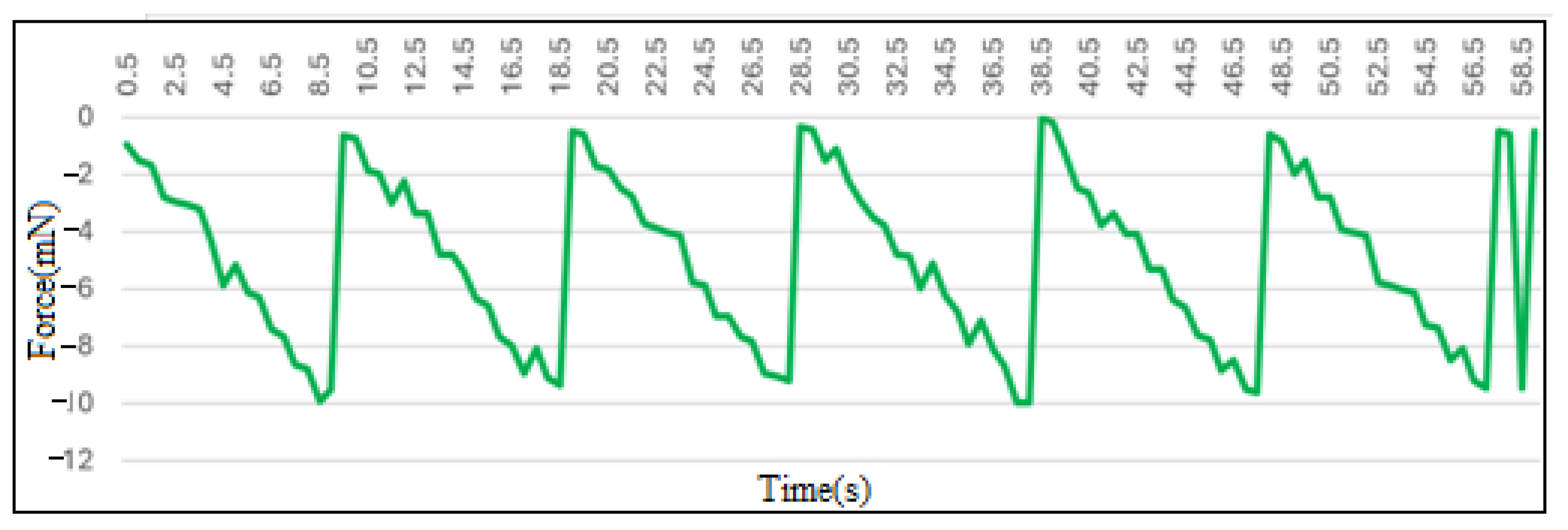
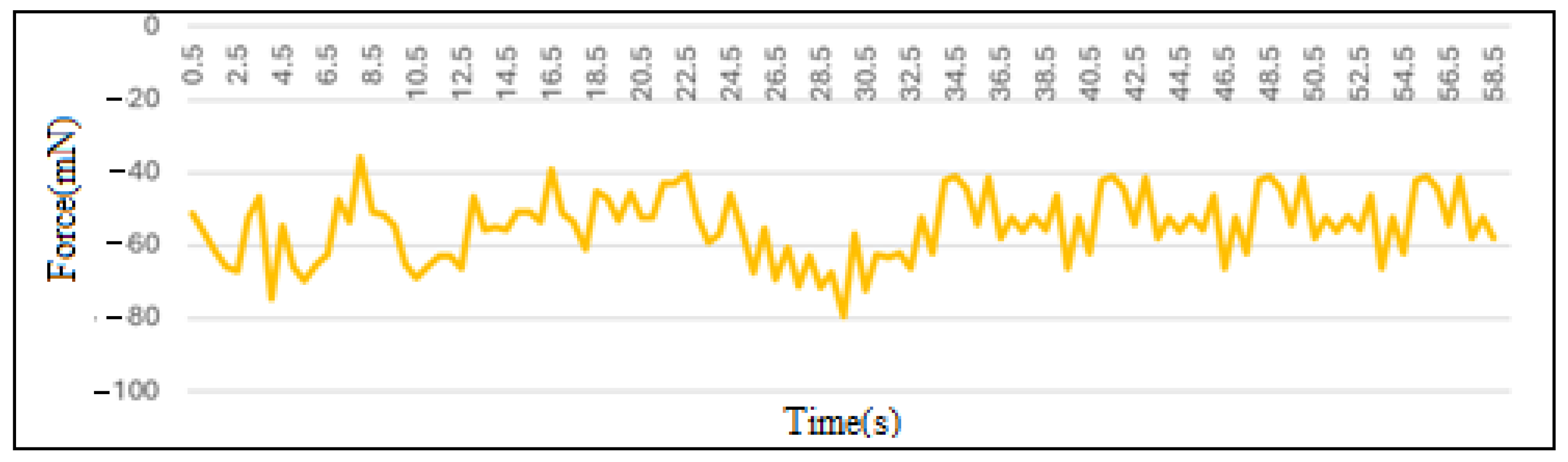
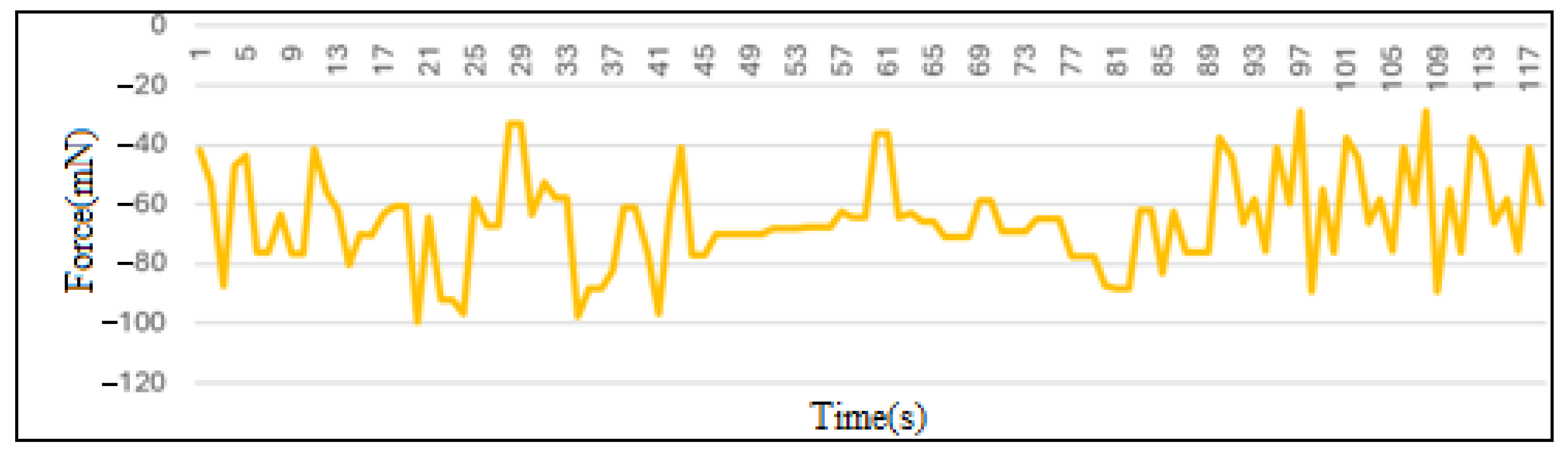
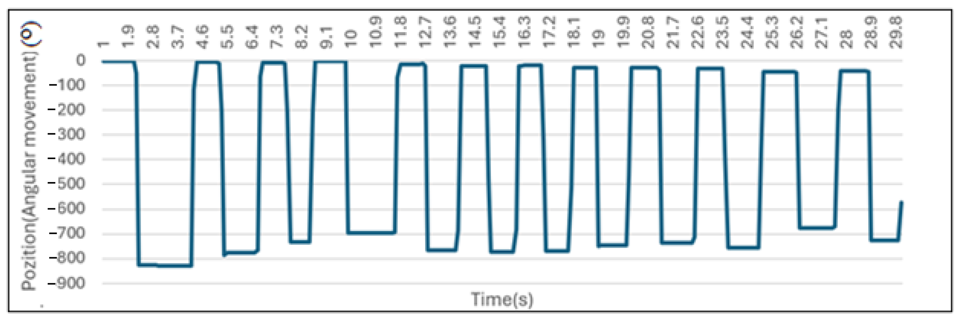
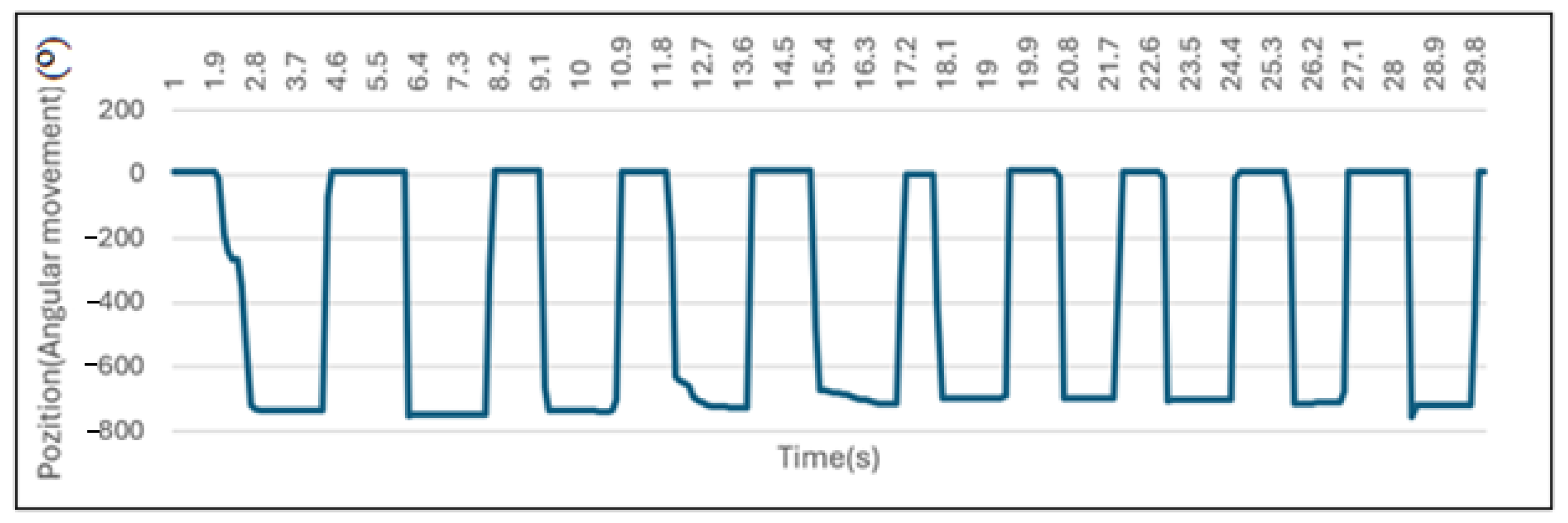
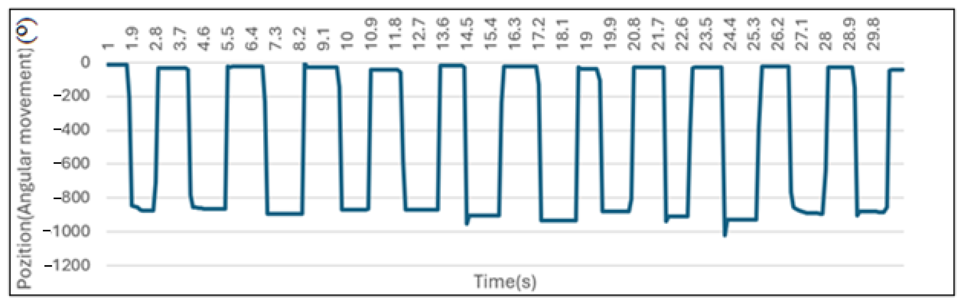
3.2. Calibrating the Slip Sensor

In this case, it is also necessary to calibrate the slip sensor for each gripping module. To calibrate the slip sensor, the following steps were necessary:

I.

Development of software for determining angular values

To determine angular values, dedicated software (Figure 23) was developed for testing, which was installed for each gripping module.

The meaning of the main instructions in this software is as follows:

-

setup() function:

pinMode(channelA, INPUT);

pinMode(channelB, INPUT);

These lines configure the digital pins channelA and channelB as digital inputs. These are the pins to which the two channels of the encoder are connected.

attachInterrupt(digitalPinToInterrupt(channelA), updateEncoder, CHANGE);

attachInterrupt(digitalPinToInterrupt(channelB), updateEncoder, CHANGE);

These lines attach interrupts to the channelA and channelB pins. digitalPinToInterrupt() converts the pin number into an interrupt identification number. attachInterrupt() sets a function (updateEncoder) that will be called every time the pin state changes (CHANGE). This allows for very fast and accurate detection of encoder state changes, without the need for constant checking in the loop() loop.

-

loop() function:

Serial.print(“Position: “);

Serial.println(position);

delay(100);

This main loop displays the current value of the variable position, which represents the encoder position, on the serial monitor. delay(100) introduces a 100-millisecond pause between displays.

-

updateEncoder() function:

This is the function that is called each time the state of the channelA or channelB pin changes.

int MSB = digitalRead(channelA);

int LSB = digitalRead(channelB);

These lines read the state of each encoder pin (0 or 1) and store them in the variables MSB (Most Significant Bit) and LSB (Least Significant Bit).

int encoded = (MSB << 1) | LSB;

This line combines the two bits into a single integer (encoded). << 1 is a bit shift to the left, which moves the MSB bit to the top position. | is a bitwise OR operation, which combines the MSB and LSB bits.

int sum = (lastEncoded << 2) | encoded;

This line combines the current encoded value with the previous value (lastEncoded). Shifting left by 2 bits (<<2) moves the previous value two places so that it can be combined with the current value.

if (sum == 0b1101 || sum == 0b0100 || sum == 0b0010 || sum == 0b1011) position++;

if (sum == 0b1110 || sum == 0b0111 || sum == 0b0001 || sum == 0b1000) position−−;

These lines detect the direction of rotation of the encoder. They compare the sum value with different combinations of bits that correspond to increasing or decreasing the position. These combinations are determined by the specific sequence of signals generated by the encoder.

lastEncoded = encoded;

This line stores the current encoded value for use on the next interrupt.

II.

Implementation and collection of read values

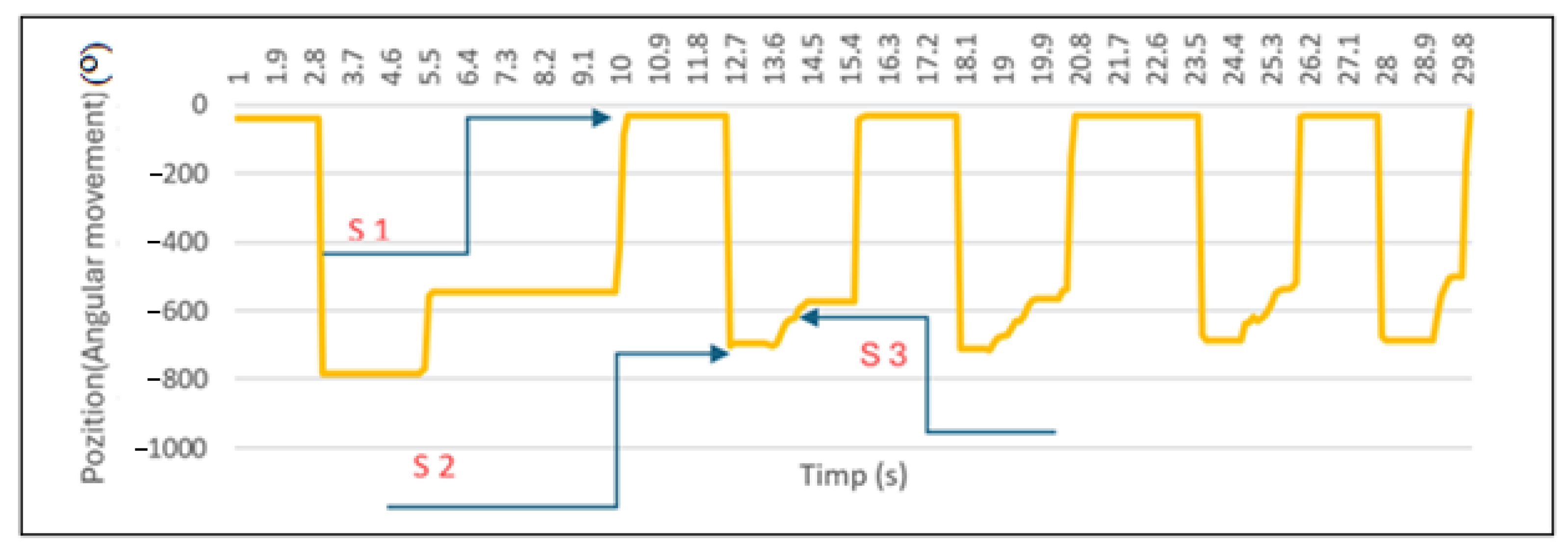
The software takes readings at a rate of 10/second to have a much higher accuracy of angular displacement measurement. The slip sensor is folded into the logical flow of the system and will be measured in the steps made in the logic diagram. To integrate the slip sensor into the sensor system, it is essential to collect data in various phases of the gripping process:

Sequence 1 (Initial Error): The background noise of the optical encoder is evaluated before contact with the object.

Table 2. Sensor error generation over a one-second interval for Module 1.

Time (s)	Angular Position (°)
0	Position: 1
0.1	Position: 1
0.2	Position: 1
0.3	Position: 1
0.4	Position: 1
0.5	Position: 1
0.6	Position: 1
0.7	Position: 1
0.8	Position: 1
0.9	Position: 1
1	Position: 1

,

Table 3. Sensor error generation over a one-second interval for Module 2.

Time (s)	Angular Position (°)
0	Position: −2
0.1	Position: −2
0.2	Position: −2
0.3	Position: −2
0.4	Position: −2
0.5	Position: −2
0.6	Position: −2
0.7	Position: −2
0.8	Position: −2
0.9	Position: −2

,

Table 4. Sensor error generation over a one-second interval for Module 3.

Time (s)	Angular Position (°)
0	Position: 7
0.1	Position: 7
0.2	Position: 7
0.3	Position: 7
0.4	Position: 7
0.5	Position: 7
0.6	Position: 7
0.7	Position: 7
0.8	Position: 7
0.9	Position: 7

,

Table 5. Sensor error generation over a one-second interval for Module 4.

Time (s)	Angular Position (°)
0	Position: −5
0.1	Position: −5
0.2	Position: −5
0.3	Position: −5
0.4	Position: −5
0.5	Position: −5
0.6	Position: −5
0.7	Position: −5
0.8	Position: −5
0.9	Position: −5

and

Table 6. Sensor error generation over a one-second interval for Module 5.

Time (s)	Angular Position (°)
0	Position: −1
0.1	Position: −1
0.2	Position: −1
0.3	Position: −1
0.4	Position: −1
0.5	Position: −1
0.6	Position: −1
0.7	Position: −1
0.8	Position: −1
0.9	Position: −1

present the error values for each module, over a one-second interval. These errors represent variations in the encoder readings in the absence of movement, probably caused by electronic noise or small vibrations.

Sequence 2 (Contact): The rotation angle of the probe is measured until contact with the object is established. Figure 24, Figure 25, Figure 26, Figure 27 and Figure 28 graphically present the angular variations over time for each module. We observe a variability in the contact angle between modules, probably due to mechanical tolerances and positioning inaccuracies. The range of values is considered as a contact threshold and is used in the control algorithm.

Sequence 3 (Sliding): The sliding of the object is manually simulated to determine the angles corresponding to the sliding. Figure 29, Figure 30, Figure 31, Figure 32 and Figure 33 illustrate the angular variations during sliding. The range of variations is used as a threshold to detect slip during normal operation. Differences between modules are due to mechanical tolerances and friction variations.

Sequence 4 (Full Cycle): A complete gripping cycle (contact, balance, slip) is analyzed to validate sensor operation and identify potential errors. Figure 34, Figure 35, Figure 36, Figure 37 and Figure 38 graphically present a complete cycle for each module. A consistency in contact detection is observed, but the need for a robust algorithm to differentiate between real slip and small position variations is highlighted.

The data collected in the four sequences are used to calibrate the slip sensor. The range of values for each sequence is defined for each module. This calibration allows the system to accurately differentiate between normal contact, equilibrium, and object slip. The variability of the results between modules highlights the need for individual calibration for each module. Further analysis demonstrates the effectiveness of the control algorithm in compensating for these variations, ensuring stable operation of the self-adaptive gripper.

Regarding the calibration of the slip sensor, the main challenge is the reproducible simulation of the slip. The manual simulation, mentioned in the text, introduces errors. Other challenges are mechanical clearances, friction, and hysteresis.

It is mentioned that the system uses a PID algorithm for each independent module of the gripper. The PID controller receives three input values: Error signal (e): It represents the difference between the desired value of the gripping force (setpoint) and the current value of the force measured by the force sensor. In the case of slip detection, the error signal reflects the difference between the desired position of the slip sensor stylus and its current position. Derivative of the error signal (de/dt): It represents the rate of change in the error signal. A high rate of change indicates a fast slip. Integral of the error signal (∫e dt): It represents the sum of the errors in the past. A high integral indicates a persistent error. Based on these three values, the PID controller calculates an output signal that adjusts the gripping force: output signal = Kp * e + Ki * ∫e dt + Kd * de/dt, where Kp (proportional gain) determines the immediate response of the system to the error. A large Kp leads to a fast response, but can cause oscillations. Ki (integral gain): Compensates for persistent errors. A large Ki reduces static error, but can cause overshoot. Kd (derivative gain): Dampens oscillations and improves system stability. A large Kd reduces overshoot, but can make the system slow.

II.1

Determining errors for each module (Sequence 1)

Table 2, Table 3, Table 4, Table 5 and Table 6 show the slip sensor errors over a one-second interval for each grip module.

II.2

Contact angle determination for each module (Sequence 2)

The measurements made by the sensor probe until the contact was established were repeated several times for the same sensor, in order to define certain thresholds in the form of intervals. The simulations were performed over a period of 30 s.

The contact simulation for Module 1 corresponds to the data of the graph in Figure 24. In this data collection process, the contact was repeated several times. According to the results, sensor 1 generates contact values between −600° and −800°, and when it is released, the values tend between 0 and −20°. The graph shows the variation in the angular position (in undefined units) of the slide sensor probe on Module 1 as a function of time (in seconds) during the contact angle determination sequence (Calibration Sequence 2). The graph shows a series of repeated cycles, each cycle likely representing one contact attempt. Each cycle has three phases: 1. Initial phase: The probe is in an initial position (approximately −400), ready for contact. 2. Contact: The probe moves rapidly to a contact position (approximately −600). The travel speed is relatively high, indicating a fast actuator. 3. Return: After contact, the probe returns to its initial position. The return speed is slower than the travel speed to contact. The data show the following: Contact angle variability: There is a slight variability in the contact angle over each cycle. This variation could be caused by variability in object positioning or other sources of error. Importance for Calibration: The data in this graph are essential for calibrating the slip sensor. Analysis of these data allows the determination of a contact threshold, defined as an angular value that indicates firm contact with the object. It also allows the evaluation of measurement reproducibility and the identification of possible mechanical or control problems.

The contact simulation for Module 2 corresponds to the data of the graph in Figure 25. In this data collection process, the contact was repeated several times. According to the results, sensor 2 generates contact values between −650° and −800°, and when it is released, the values tend between 0 and −50°.

The contact simulation for Module 3 corresponds to the data of the graph in Figure 26.

In this data collection process, the contact was repeated several times. According to the results, sensor 3 generates contact values between −650°−750°, and when released, the values tend between 0 and 20°.

The contact simulation for Module 4 corresponds to the data in the graph in Figure 27. In this data collection process, the contact was repeated several times. According to the results, sensor 4 generates contact values between −800°−1000°, and when released, the values tend between 0 and −50°.

The contact simulation for Module 5 corresponds to the data in the graph in Figure 28.

In this data collection process, the contact was repeated several times. According to the results, sensor 5 generates contact values between 600° and 750°, and upon release, the values tend between 0 and −30°. As can be seen, the contact values are positive compared to the values generated by the other sensors. This aspect will not influence the grip, because in the software, only positive values will be declared, even if they are generated as negative measurements.

II.3

Determining the angular values indicating the sliding of the grasped object (Sequence 3)

The graphs show the variation in the angular position (expressed in degrees) of the slide sensor probe on each module over a period of 30 s. The horizontal axis represents time (in seconds), and the vertical axis represents the angular position (in undefined units, but assuming degrees). The line of the graph illustrates the movement of the probe during the simulation of an object sliding. The graphs show a series of cycles, each cycle presumably representing a simulation of the object sliding. Each cycle has three main phases:

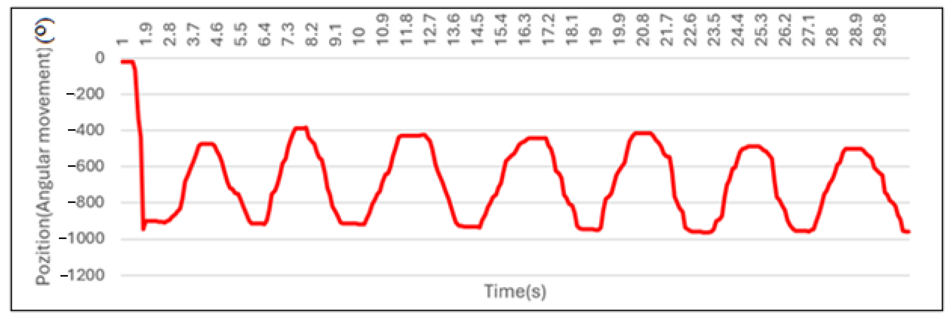
• Rest phase: The probe is maintained in a relatively stable position, around −750 degrees. This represents the initial position of the sensor, before the simulation;
• Sliding phase: A sudden decrease in the angular position of the probe is observed, indicating a relatively rapid movement of the object. This represents the simulation of the object sliding. The amplitude of the decrease is variable from one cycle to another, probably due to variations in the friction force or other factors.
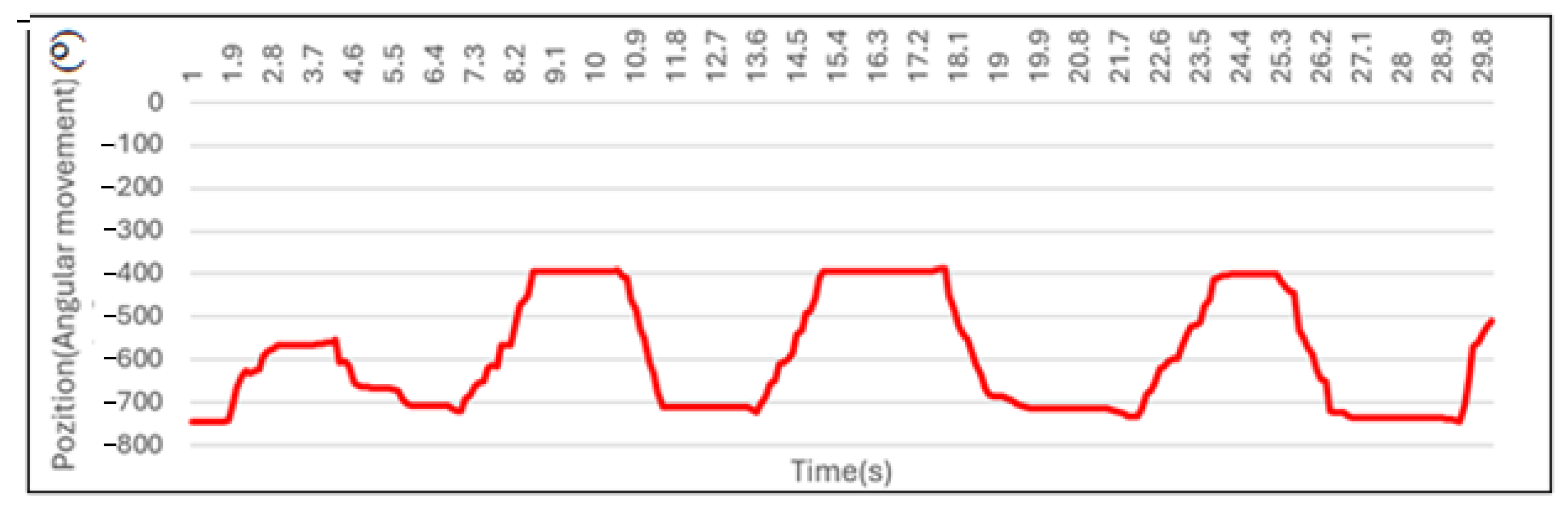
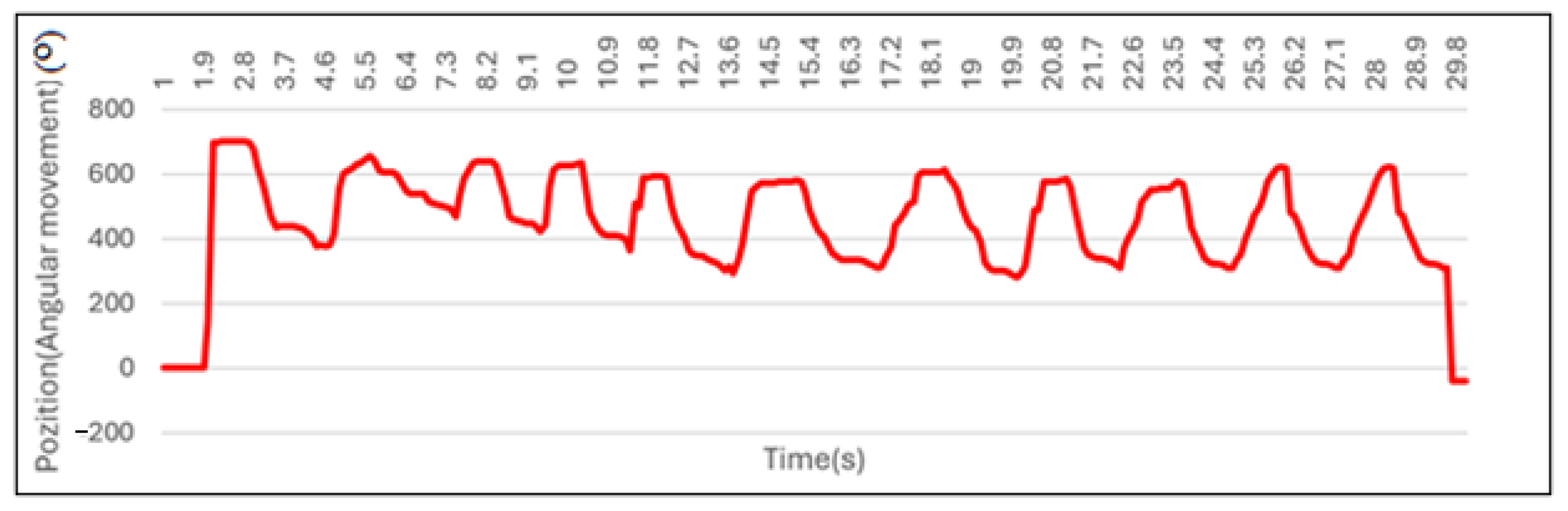
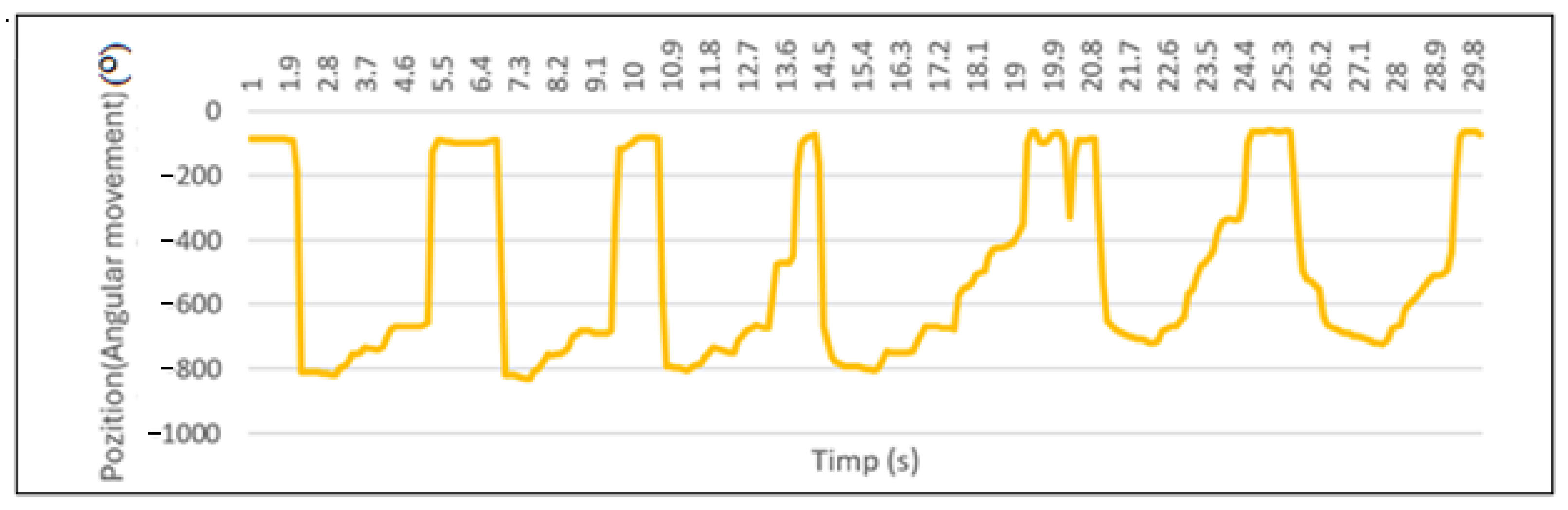
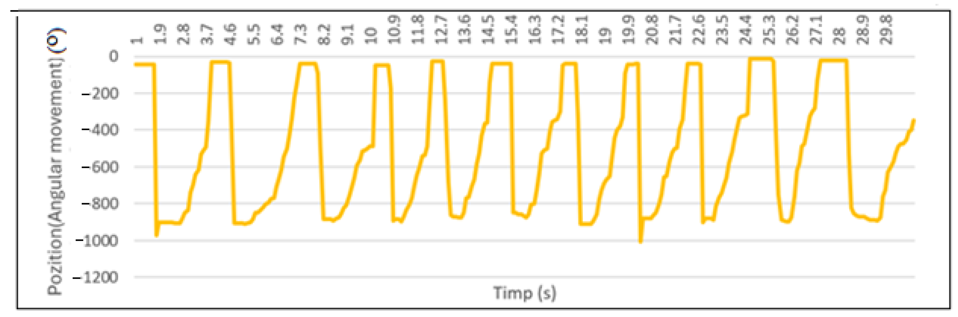
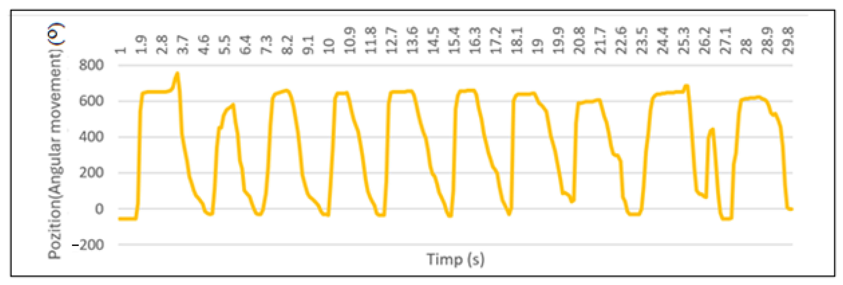
• Recovery phase: After the slip, the probe returns to its initial position (−750 degrees), but not necessarily to the same position as at the beginning of the cycle. The sudden decrease in the angular position of the probe indicates a relative movement between the probe and the object, representing the object slipping. The amplitude of this decrease is an indicator of the magnitude of the slip. Variability in amplitude from one cycle to another suggests that either the sliding force or the friction conditions varied during the simulation. For example, if the object has a rougher surface, the slip will be smaller. To evaluate the slip values, the probe was kept in constant contact, and the slip was simulated manually, moving in the gravitational direction, without the object detaching from the sensor jaws. Measurements were performed over a period of 30 s, during which various slips were simulated to establish a specific range in which the slip occurs for each grip module. The simulation of the slip of Module 1 corresponds to the data presented in the graph in Figure 29. During the slip, it is observed that, from the contact position of −750, the value decreases to −400. This difference represents the maximum slip allowed for sensor 1. The slip range for sensor 1 is between −750 and −400. The simulation of the sliding of Module 2 corresponds to the data shown in the graph in Figure 30. During the sliding, it is observed that, from the contact position of −900, the value decreases to −400. This difference represents the maximum allowed sliding for sensor 2. The sliding range for sensor 2 is between −900 and −350. The simulation of the sliding of Module 3 corresponds to the data shown in the graph in Figure 31.

During the sliding, it is observed that, from the contact position of −700, the value decreases to −400. This difference represents the maximum allowed sliding for sensor 3.

The sliding range for sensor 3 is between −700 and −100. The simulation of the sliding of Module 4 corresponds to the data shown in the graph in Figure 32. During the sliding, it is observed that, from the contact position of −950, the value decreases to −400. This difference represents the maximum allowed slip for sensor 4. The slip range for sensor 4 is between −950 and −400. The simulation of the slip of Module 5 corresponds to the data presented in the graph in Figure 33. During the slip, it is observed that, from the contact position of (700), the value decreases to −400. This difference represents the maximum allowed slip for sensor 5. The slip range for sensor 5 is between 700 and 300. The differences in frequency of results over the same time interval are caused by the way the simulations were performed: by applying contact of an object to each trough, while the slip simulation was performed manually.

II.4

Determining the angular values for a complete sequence at the slip sensor

The calibration of the slip sensor involved simulating several complete gripping cycles over a period of 30 s, in order to identify the angular ranges specific to each sequence. Data analysis revealed three distinct sequences in each cycle:

Sequence 1—Free state (range 10–12.5 s): Before contact, the sensor is in a resting position, with stable angular values;

Sequence 2—Contact (12.6–13.5 s): The establishment of contact with the object is marked by a sudden increase in the angular value (approximately −800°), followed by a short period of equilibrium;

Sequence 3—Slip (13.5–15.4 s): The slipping of the object is evidenced by a gradual decrease in the angular value, starting from the equilibrium point. This sequence of events (free state, contact, slip) is repeated during the simulation, providing sufficient data to define the angular threshold that indicates slipping.

Repeating measurements over a period of 30 s allowed for statistical analysis of the data and a more precise determination of the angular intervals for each phase of the gripping cycle.

The simulation of the cycles of Module 1 corresponds to the data presented in Figure 34.

According to the collected data, three sequences are observed at each cycle performed. The system starts collecting data when the sensor is, for a short period of time (interval s9.8–s12), in a free state, followed by a large angular value (−800°), which represents the contact; in the contact position, it remained in equilibrium for a short period of time (s12.1–s13.5), followed by a gradual angular decrease representing the slip (s13.5–s15.3).

The simulation of the Module 2 cycles corresponds to the data presented in the graph in Figure 35.

According to the collected data, three sequences are observed at each cycle performed. The system starts collecting data when the sensor is, for a short period of time (interval s5.4–s6.5), in a free state, followed by a large angular value (−800°) which represents the contact; in the contact position, it remained in equilibrium for a short period of time (s6.6–s7.6), followed by a gradual angular decrease which represents the slip (s7.6–s9.8).

The simulation of the Module 3 cycles corresponds to the data presented in the graph in Figure 36.

According to the collected data, three sequences are observed at each cycle performed. The system starts collecting data when the sensor is, for a short period of time (interval s 3.3-s4.4), in the free state, followed by a large angular value (−700°) which represents the contact; in the contact position, it remained in equilibrium for a short period of time (s4.5–s6.3), followed by a gradual angular decrease which represents the slip (s6.3 –s7.6).

The simulation of the Module 4 cycles corresponds to the data presented in the graph in Figure 37.

According to the collected data, three sequences are observed at each cycle performed. The system starts collecting data when the sensor is, for a short period of time (interval s4.1–s4.4), in the free state, followed by a large angular value (−850°), which represents the contact; in the contact position, it remained in equilibrium for a short period of time (s4.5–s5.4), after which a gradual angular decrease follows which represents the sliding (s5.4–s7.3).

The simulation of the Module 5 cycles corresponds to the data presented in the graph in Figure 38.

According to the collected data, three sequences are observed at each cycle performed. The system starts collecting data when the sensor is in a free state for a short period of time (interval s4.9–s5.3), followed by a large angular value (650°), which represents contact; in the contact position, it remained in equilibrium for a short period of time (s5.4–s5.9), followed by a gradual angular decrease representing sliding (s5.9–s7.0).

The graphs above present, at such a level of detail rarely encountered in studies in the field, the complexity of the calibration process, the differences between the five gripping modules, which require individual calibration, and the usefulness of calibration to ensure the safe operation of the designed and tested adaptive gripper, which requires the presentation of these situations in the case of other gripping systems, so as to demonstrate the innovative nature of the research.

3.3. Testing the Grip for Implementation in Real Operations

For real testing and simulation of grip quality, two types of solid objects were used—pieces with irregular shapes, for testing the effectiveness of the gripper and the performances of the sensors used. Figure 39a shows object number 1 used for the actual testing of the self-adaptive grip, and Figure 39b shows its grip position.

Figure 40a shows object number 2, and Figure 40b shows its grasping with the self-adaptive gripper (b).

The grasping was successfully performed, with each module of the grasper operating independently and correctly. In the following stages, it is necessary to optimize each module, a process that involves adjustments to the software specific to each module, depending on the data coming from its sensors. This optimization will contribute to improving the grasping process. All tests were performed without the grasper executing additional movements that would introduce inertial forces on the object or modules. Creating a well-defined logical architecture, with independent controllers for each grasper module, facilitated the implementation of self-adaptability. Individual control of the modules and quick decisions made by the Master controller contributed to the adaptability and reliability of the grasper under different grasping conditions. Implementing an efficient communication structure between the Master controller and the Slave modules allowed for precise and synchronized coordination of the grasping process. The ability to transmit simultaneous commands and collect essential data about the status of each module contributed significantly to the overall performance of the grasper. The implementation of a Master–Slave scheme in the gripper communication allows for centralized gripper control, ensuring efficient management of each module according to its specific status and requirements. This logical structure facilitates fast and accurate decisions-making during the gripper processes, contributing to the adaptability and efficiency of the system. The design and implementation of the control panel scheme facilitated precise control of the gripper, including the initiation, monitoring, and adjustment of the gripper according to the requirements of each object. In summary, the adaptive gripper, equipped with a PID algorithm system for each module, handles objects with irregular and unpredictable shapes through a combination of the following:

• Individual module control (each module has its own force sensor and its own PID controller). This allows for independent adaptation to the shape of the object. The modules adjust individually to conform to the contour of the object, ensuring multiple contact and uniform distribution of gripping force;
• Slip detection and compensation: Slip sensors instantly detect any unexpected movement of the object. The PID controller reacts immediately by adjusting the gripping force to prevent slipping.

The rate of force change is controlled by the derivative component of the PID controller, ensuring a fast and precise response. Gripping force adaptation: Force sensors measure the gripping force applied to the object. The PID controller continuously adjusts the clamping force to maintain it at the desired value, compensating for variations in the shape and weight of the object. The integral PID controller component ensures precise compensation of persistent errors. Advanced control algorithms (potentially): Depending on the complexity of the implementation, more advanced control algorithms such as model-based control or machine learning algorithms could be used to improve the ability to adapt to complex and unpredictable shapes. This electrical and software integration ensured an efficient interaction between the operator and the gripper system, significantly contributing to achieving the objectives of adaptability and correct operation of the gripper.

4. Conclusions

The logical architecture of the sensory system is designed to allow independent mechanical, electrical, and software understanding. The implementation of the three-step self-adaptive grasping ensures precise object handling, avoiding their slipping and deformation.

The sliding sensor system implemented in the self-adaptive gripper jaw uses a resistive encoder and a flat strip with translational and rotational movement to detect and manipulate objects. It ensures efficient and safe gripping, minimizing slipping and deformation of grasped objects.

Software tests of the sensor system confirm the correct functionality of the resistive encoder in detecting the position and small errors. Implementation of a high-resolution optical incremental encoder and optimization of the translation and rotation mechanism are recommended to improve the performance and reliability of the system.

The design of the advanced robotic gripper focused on the integration of a slip sensor to improve the ability to grip and manipulate objects, emphasizing the importance of geometric and material optimization for performance and durability.

The implementation and testing of the advanced robotic gripper demonstrated its efficiency and functionality under real-world conditions, confirming its ability to adapt and perform precise operations in various industrial and object-handling applications.

5. Future Works

Tests to optimize the gripper’s operation will continue with parts of other shapes and sizes, with the gripper being mounted on a Cartesian robot that will be integrated into a robotic assembly line of subassemblies used in the automotive industry.

Future improvements to the sensor system, with a view to further implementing machine learning (AI) functionalities, focus on the following:

Advanced sensor integration: Higher-resolution and -precision force sensors: Replacing existing force sensors with higher-resolution and improved-precision sensors, reducing measurement noise and increasing the accuracy of force detection. Sensors with integrated thermal compensation will improve reliability in various environmental conditions. Higher-resolution incremental optical encoders: Using higher-resolution encoders to improve the accuracy of measuring probe movement, reducing slip detection errors. Speed sensors: Adding speed sensors to measure the slip rate, improving the accuracy of control algorithms and allowing faster reaction to slip. Proximity sensors: Integrating proximity sensors to detect the approach of the object before contact, allowing for more precise gripping and avoiding collisions. Computer vision: Integrating a camera to obtain visual information about the shape and orientation of the object. These data can be used by machine learning algorithms for a more precise and robust grip.

-

Improving data processing algorithms: Implementing more sophisticated digital filtering techniques (e.g., Kalman filters, weighted moving average filters) to reduce noise in sensory data and improve measurement accuracy; combining data from different sensors (force, slip, computer vision) to obtain a more complete picture of the system state and improve the accuracy and reliability of slip detection.

-

Implementing machine learning (AI) algorithms: Training a machine learning model by imitating the movements of a human operator manipulating objects. The model will learn to adapt the gripping force and movements depending on the shape and texture of the object; Using reinforcement learning techniques to optimize the parameters of the control algorithm and improve the performance of the gripper in various situations. The algorithm will learn to adjust the gripping force and movements based on feedback from the environment; Using shape classification techniques to automatically identify the shape of the object and adapt the gripping strategy. Computer vision is essential for this functionality; Training a machine learning model to predict slippage before it occurs, allowing for a preventive reaction.

The operation of the adaptive gripper in high-speed industrial applications requires specific optimizations to ensure robustness and reliability by adapting to high speeds with appropriate solutions. The following are subjects of future research: the use of force and slip sensors with a very short response time; the PID algorithm, optimized for high processing speeds; the replacement of the stepper motor with a faster drive system, such as a servo motor with precise position and speed control; the inclusion of robust error management, covering the detection of communication errors, sensor failures, and other unexpected events; and the implementation of redundant mechanisms to ensure system operation even in the event of failure of one or more modules.

References

1. Available online: https://robotiq.com/ (accessed on 14 October 2024).
2. Manz, M.; Bartsch, S.; Simnofske, M.; Kirchner, F. Development of a Self-Adaptive Gripper and Implementation of a Gripping Reflex to Increase the Dynamic Payload Capacity. In Proceedings of the ISR 2016, 47st International Symposium on Robotics, Munich, Germany, 21–22 June 2016; pp. 56–62. [Google Scholar]
3. Ceccarelli, M.; Figliolini, G.; Ottaviano, E.; Mata, A.S.; Criado, E.J. Designing a robotic gripper for harvesting horticulture products. Robotica 2000, 18, 105–111. [Google Scholar] [CrossRef]
4. Carbone, G.; Ceccarelli, M. Design of LARM hand: Problems and solutions. Control. Eng. Appl. Inform. 2008, 10, 39–46. [Google Scholar]
5. Backus, B.S.; Dollar, M.A. An Adaptive Three-Fingered Prismatic Gripper With Passive Rotational Joints. IEEE Robot. Autom. Lett. 2016, 1, 668–675. [Google Scholar] [CrossRef]
6. Tang, S.; Yu, Y.; Sun, S.; Li, Z.; Sarkodie-Gyan, T.; Li, W. Design and experimental evaluation of a new modular underactuated multi-fingered robot hand. Proc. Inst. Mech. Eng. Part C J. Mech. Eng. Sci. 2020, 234, 3709–3724. [Google Scholar] [CrossRef]
7. Chapman, J.; Gorjup, G.; Dwivedi, A.; Matsunaga, S.; Mariyama, T.; MacDonald, B.; Liarokapis, M. A Locally-Adaptive, Parallel-Jaw Gripper with Clamping and Rolling Capable, Soft Fingertips for Fine Manipulation of Flexible Flat Cables. In Proceedings of the IEEE International Conference on Robotics and Automation (ICRA), Xi’an, China, 18 October 2021; pp. 6941–6947. [Google Scholar] [CrossRef]
8. Wan, W.; Harada, K.; Kanehiro, F. Planning Grasps With Suction Cups and Parallel Grippers Using Superimposed Segmentation of Object Meshes. IEEE Trans. Robot. 2021, 37, 166–184. [Google Scholar] [CrossRef]
9. Parada Puig, J.E.; Nava Rodriguez, N.E.; Ceccarelli, M. A Methodology for the Design of Robotic Hands with Multiple Fingers. Int. J. Adv. Robot. Syst. 2008, 5, 177–184. [Google Scholar]
10. Costanzo, M.; De Maria, G.; Natale, C.; Pirozzi, S. Design and Calibration of a Force/Tactile Sensor for Dexterous Manipulation. Sensors 2019, 19, 966. [Google Scholar] [CrossRef] [PubMed]
11. Han, Y.; Jing, B.; Chirikjian, G. Design, Calibration, and Control of Compliant Force-sensing Gripping Pads for Humanoid Robots. J. Mech. Robot. 2023, 15, 031010. [Google Scholar] [CrossRef]
12. Cortinovis, S.; Vitrani, G.; Maggiali, M.; Romeo, R.A. Control Methodologies for Robotic Grippers: A Review. Actuators 2023, 12, 332. [Google Scholar] [CrossRef]
13. Romeo, R.; Zollo, L. Methods and Sensors for Slip Detection in Robotics: A Survey. IEEE Access 2020, 8, 73027–73050. [Google Scholar] [CrossRef]
14. De Clercq, T.; Sianov, A.A.; Crevecoeur, G. A Soft Barometric Tactile Sensor to Simultaneously Localize Contact and Estimate Normal Force with Validation to Detect Slip in a Robotic Gripper. IEEE Robot. Autom. Lett. 2022, 7, 11767–11774. [Google Scholar] [CrossRef]
15. Itu, A.; Staretu, I.; Danciu, G. Automatic Grasp Planning Using Grasping Strategies. In Proceedings of the 4-th International Conference on Robotics-Robotica, Guangzhou, China, 17–19 November 2008; pp. 407–412. [Google Scholar]
16. Itu, A.; Staretu, I.; Danciu, G. Developing a Control Interface for a Three Fingered Gripper. In Proceedings of the 4-th International Conference on Robotics-Robotica 2008, Pasadena, CA, USA, 19–23 May 2008; pp. 412–416. [Google Scholar]
17. Kim, D.; Park, S. Software Architecture-based Approach to Self-adaptive Function for Intelligent Robots. IFAC 2008, 41, 5297–5302. [Google Scholar] [CrossRef]
18. Cheng, L.-W.; Liu, S.-W.; Chang, J.-Y. Design of an Eye-in-Hand Smart Gripper for Visual and Mechanical Adaptation in Grasping. Appl. Sci. 2022, 12, 5024. [Google Scholar] [CrossRef]
19. Kakani, V.; Cui, X.; Ma, M.; Kim, H. Vision-Based Tactile Sensor Mechanism for the Estimation of Contact Position and Force Distribution Using Deep Learning. Sensors 2021, 21, 1920. [Google Scholar] [CrossRef] [PubMed]
20. Kumar, A.; Kumar, A.L.; Aravindan, V.; Arunachallam, R. Robotic Gripper With Force Feedback System. IOP Conf. Ser. Mater. Sci. Eng. 2020, 912, 032049. [Google Scholar] [CrossRef]
21. Kuang, L.; Lou, Y.; Song, S. Design and Fabrication of a Novel Force Sensor for Robot Grippers. IEEE Sens. J. 2018, 18, 1410–1418. [Google Scholar] [CrossRef]
22. Xu, W.; Zhang, H.; Yuan, H.; Liang, B. A Compliant Adaptive Gripper and Its Intrinsic Force Sensing Method. IEEE Trans. Robot. 2021, 37, 1584–1603. [Google Scholar] [CrossRef]
23. Veeramuthu, L.; Weng, R.J.; Chiang, W.H.; Pandiyan, A.; Liu, F.J.; Liang, F.C.; Kumar, G.R.; Hsu, H.-Y.; Chen, Y.-C.; Lin, W.-Y.; et al. Bio-inspired sustainable electrospun quantum nanostructures for high quality factor enabled face masks and self-powered intelligent theranostics. Chem. Eng. J. 2024, 502, 157752. [Google Scholar] [CrossRef]
Figure 1. Logical operating architecture of a gripper module.
Applsci 15 03098 g001
Figure 2. The components of the slip sensor (a) and the transmission of movement to the encoder (b). 1. Component for returning to position 0; 2. Extension spring for return to 0 position; 3. Probe translation axis; 4. Translation shaft guide bushing; 5. Flat-type probe; 9. Rack type shaft; 10. Pinion; 9-10 rack-and-pinion system; 11. Anti-rotation guide.
Applsci 15 03098 g002
Figure 3. Detail of the probe retraction mechanism (a), section through the slip sensor (b), and isometric representation of the slip sensor assembly (c). 1. Encoder; 2. Encoder support; 12. Encoder shaft; 14. Extension spring.
Applsci 15 03098 g003
Figure 4. CAD design of the slip sensor assembly (a), left side view (b) and right side view of the slip sensor assembly (c).
Applsci 15 03098 g004
Figure 5. FEM analysis of the gripping module (a), position and size of the force sensor support piece (b), component parts of the force sensor support piece (c), and CAD shape of the adaptive gripper highlighting the force sensor support pieces marked 1 (d).
Applsci 15 03098 g005
Figure 6. General electro-electronic diagram (a) and the corresponding practically realized version (b) and adaptive gripper designed (c). 1. Motor driver; 2. 12v power supply; 3. Slave Controler; 4. Master Controler; 5. RGB LED; 6. Encoder; 7. Force sensor; 8. Stepper motor.
Applsci 15 03098 g006aApplsci 15 03098 g006b
Figure 7. Direction of force application on the contact jaw of the gripping module.
Applsci 15 03098 g007
Figure 8. Noise (mechanical stress) of Module 1 over a one-minute period, Phase 1.
Applsci 15 03098 g008
Figure 9. Results of Gripping Module 1, Phase 2.
Applsci 15 03098 g009
Figure 10. Results of Gripping Module 1, Phase 3.
Applsci 15 03098 g010
Figure 11. Results of Gripping Module 2, Phase 1.
Applsci 15 03098 g011
Figure 12. Results of Gripping Module 2, Phase 2.
Applsci 15 03098 g012
Figure 13. Results of Gripping Module 2, Phase 3.
Applsci 15 03098 g013
Figure 14. Results of Gripping Module 3, Phase 1.
Applsci 15 03098 g014
Figure 15. Results of Gripping Module 3, Phase 2.
Applsci 15 03098 g015
Figure 16. Results of Gripping Module 3, Phase 3.
Applsci 15 03098 g016
Figure 17. Results of Gripping Module 4, Phase 1.
Applsci 15 03098 g017
Figure 18. Results of Gripping Module 4, Phase 2.
Applsci 15 03098 g018
Figure 19. Results of Gripping Module 4, Phase 3.
Applsci 15 03098 g019
Figure 20. Results of Gripping Module 5, Phase 1.
Applsci 15 03098 g020
Figure 21. Results of Gripping Module 5, Phase 2.
Applsci 15 03098 g021
Figure 22. Results of Gripping Module 5, Phase 3.
Applsci 15 03098 g022
Figure 23. Software for testing angular variation.
Applsci 15 03098 g023
Figure 24. Contact angle determination in ° over a time interval for Module 1.
Applsci 15 03098 g024
Figure 25. Contact angle determination in ° over a time interval for Module 2.
Applsci 15 03098 g025
Figure 26. Contact angle determination in ° over a time interval for Module 3.
Applsci 15 03098 g026
Figure 27. Contact angle determination in ° over a time interval for Module 4.
Applsci 15 03098 g027
Figure 28. Contact angle determination in ° over a time interval for Module 5.
Applsci 15 03098 g028
Figure 29. Angular determination of slip in ° over a time interval for Module 1.
Applsci 15 03098 g029
Figure 30. Angular determination of slip in ° over a time interval for Module 2.
Applsci 15 03098 g030
Figure 31. Angular determination of slip in ° over a time interval for Module 3.
Applsci 15 03098 g031
Figure 32. Angular determination of slip in ° over a time interval for Module 4.
Applsci 15 03098 g032
Figure 33. Angular determination of slip in ° over a time interval for Module 5.
Applsci 15 03098 g033
Figure 34. Determining the values of slip cycles in ° in a time interval for Module 1.
Applsci 15 03098 g034
Figure 35. Determining the values of slip cycles in ° in a time interval for Module 2.
Applsci 15 03098 g035
Figure 36. Determining the values of slip cycles in ° in a time interval for Module 3.
Applsci 15 03098 g036
Figure 37. Determining the values of slip cycles in ° in a time interval for Module 4.
Applsci 15 03098 g037
Figure 38. Determining the values of slip cycles in ° in a time interval for Module 5.
Applsci 15 03098 g038
Figure 39. Object number 1 used in testing (a) and its gripping position (b).
Applsci 15 03098 g039
Figure 40. Object number 2 (a) and bottom view of the grasp of object number 2 (b).
Applsci 15 03098 g040