
A Multiscale Compositional Numerical Study in Tight Oil Reservoir: Incorporating Capillary Forces in Phase Behavior Calculation

 , ,
, ,  , ,
, ,
Abstract
1. Introduction
2. Materials and Methods
2.1. The Phase Equilibrium Calculation Theory Considers the Capillary Force Effect
2.2. Multiscale Compositional Model
2.2.1. Basis Model
- The reservoir consists of three phases: oil (denoted by subscript l), gas (subscript v), and water (subscript w).
- The component model considers these three flowing phases. The water phase contains only the water component and does not achieve phase equilibrium with the other phases, whereas phase equilibrium is established among m components in the oil and gas phases.
- Fluid flow follows Darcy’s law.
- The reservoir is isothermal.
- Phase equilibrium is achieved instantaneously.
2.2.2. Sequential Formulation
2.2.3. Improved Multiscale Formulation
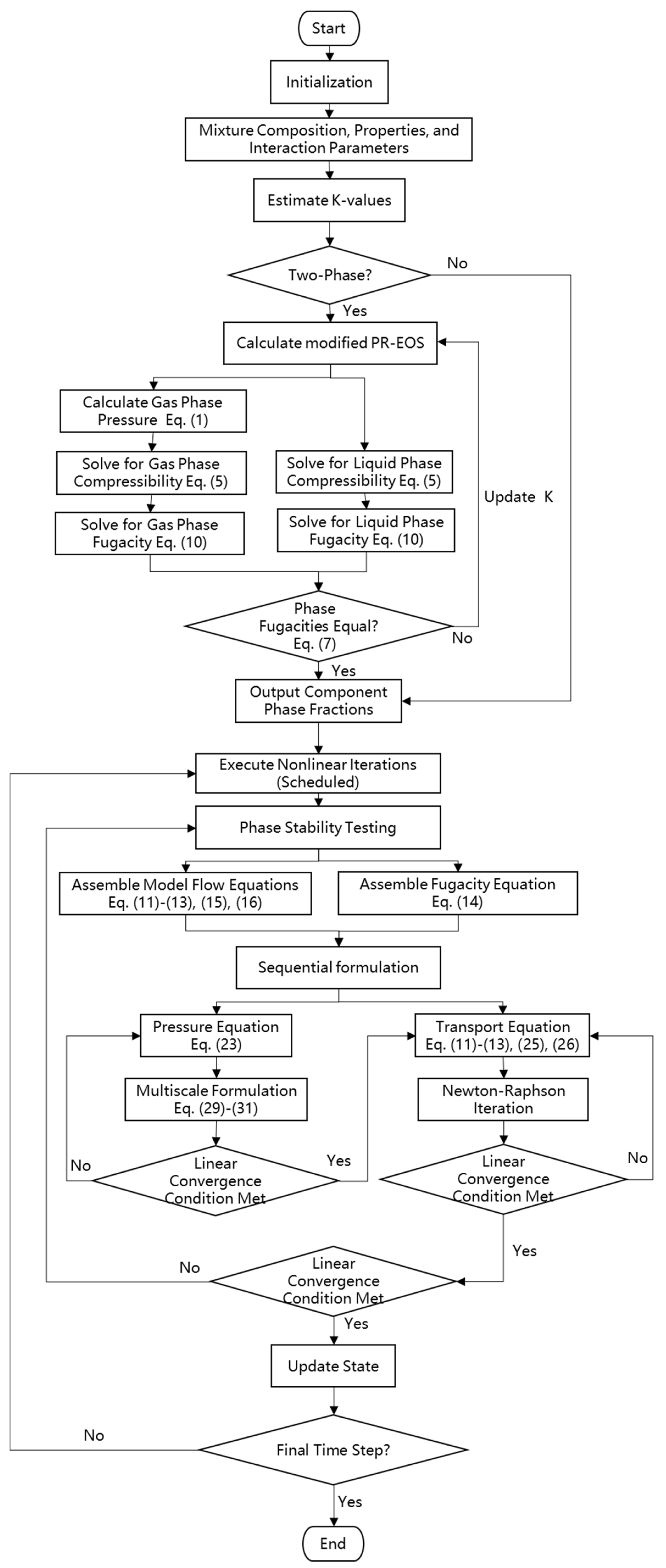
2.3. Implementation of the Multiscale Compositional Simulator
3. Results and Discussion
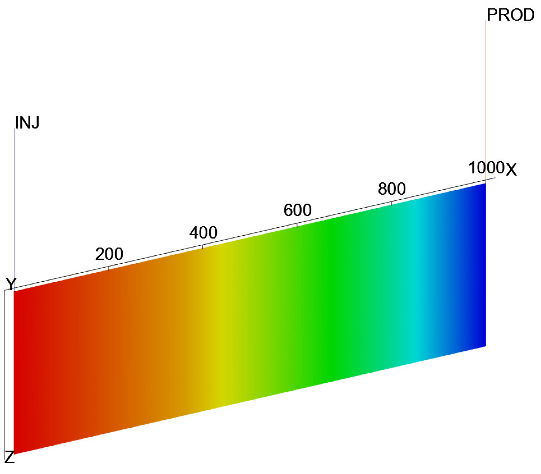
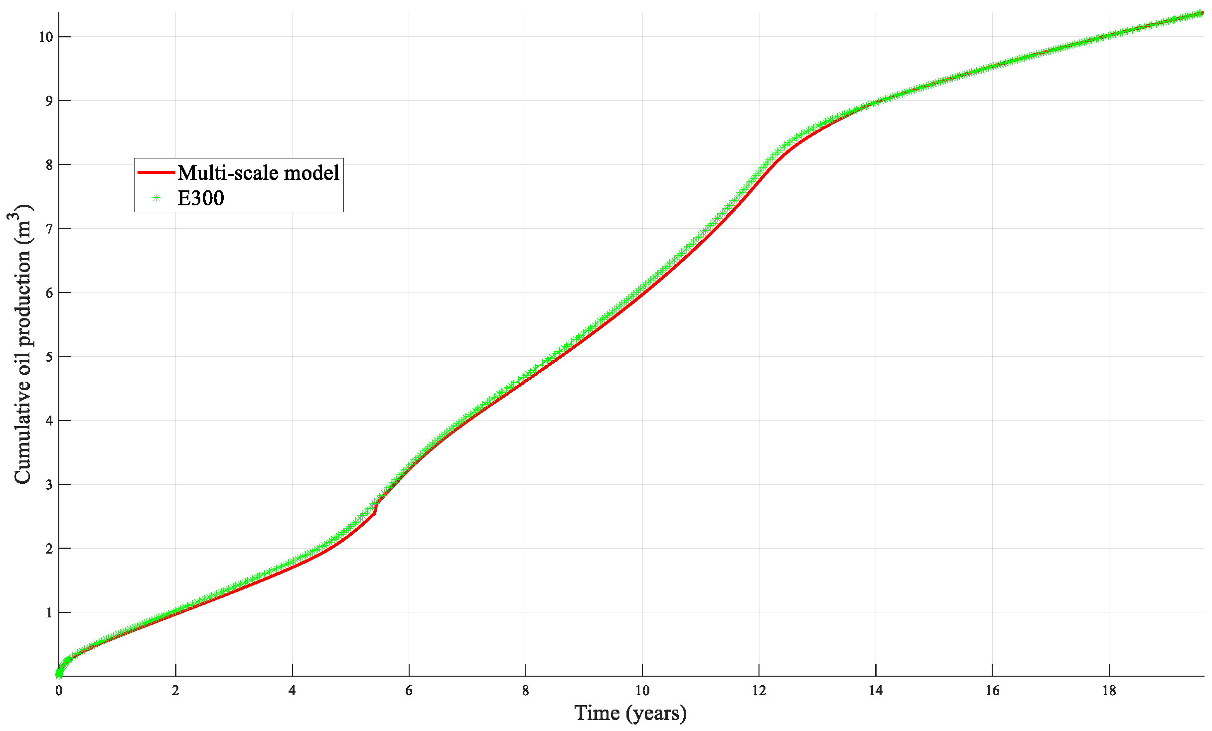
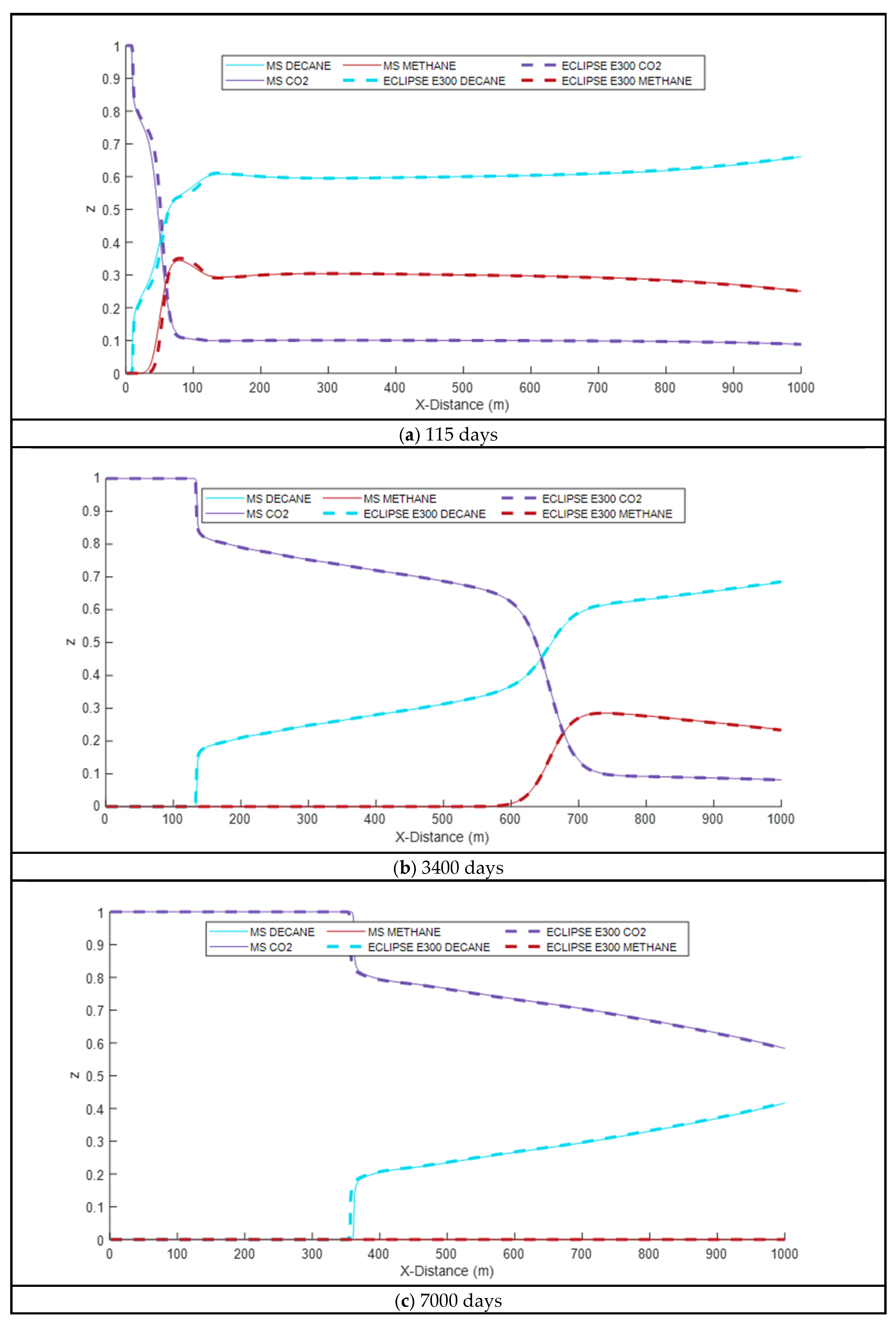
3.1. Simulation Validation
3.2. Sensitivity Analysis
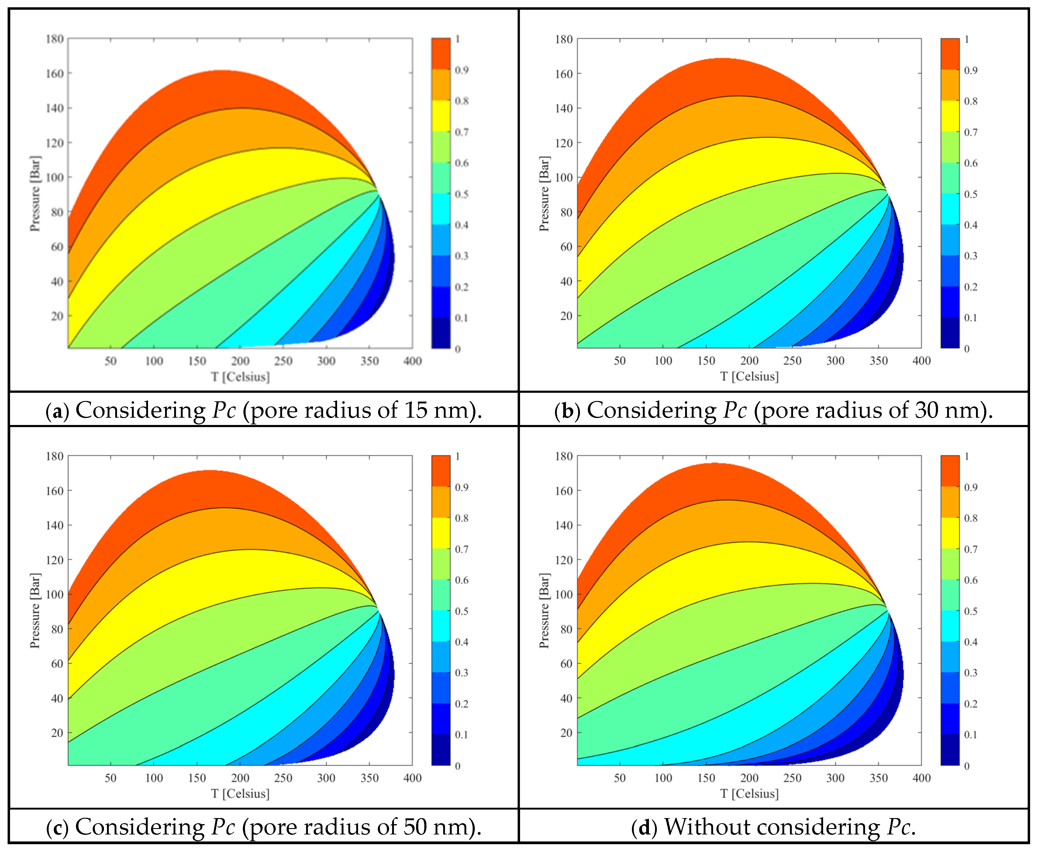
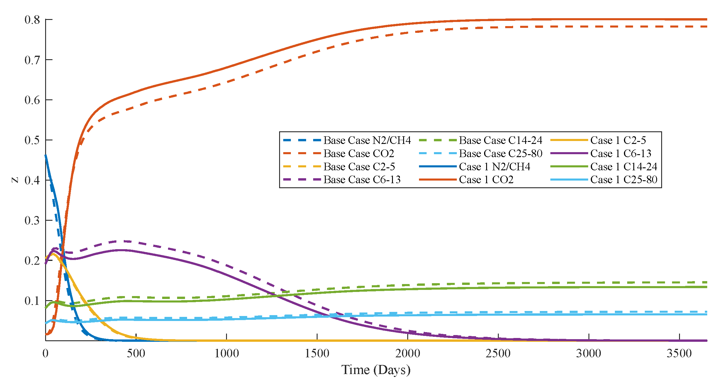
3.2.1. The Influence of Capillary Forces on Phase Equilibrium Calculations
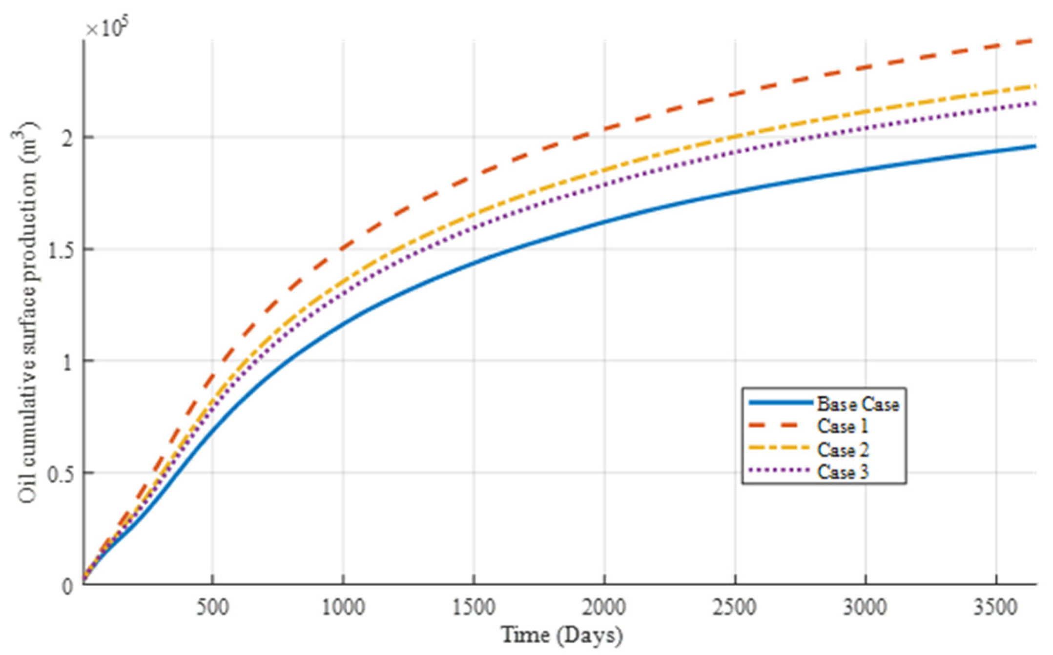
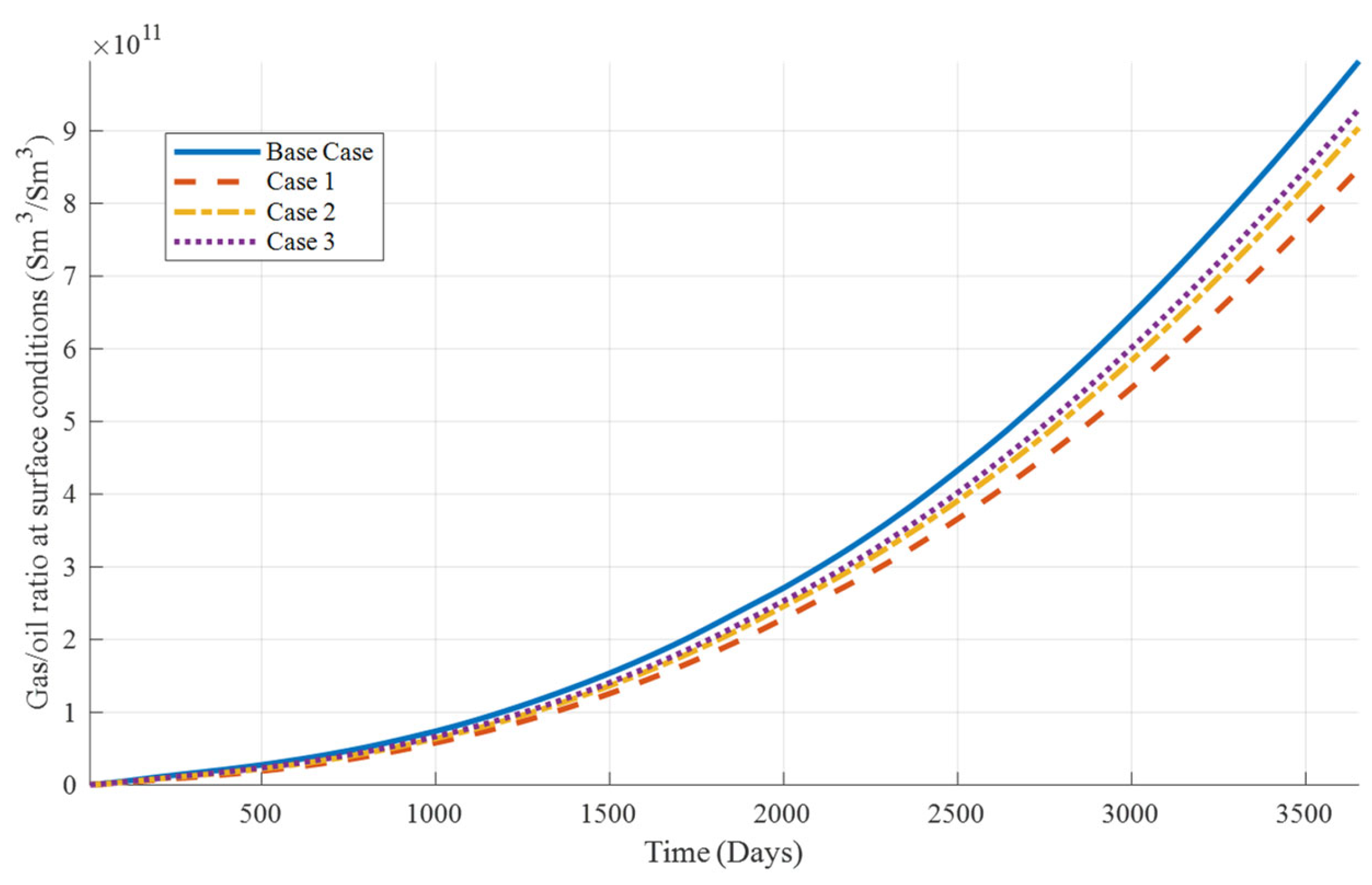
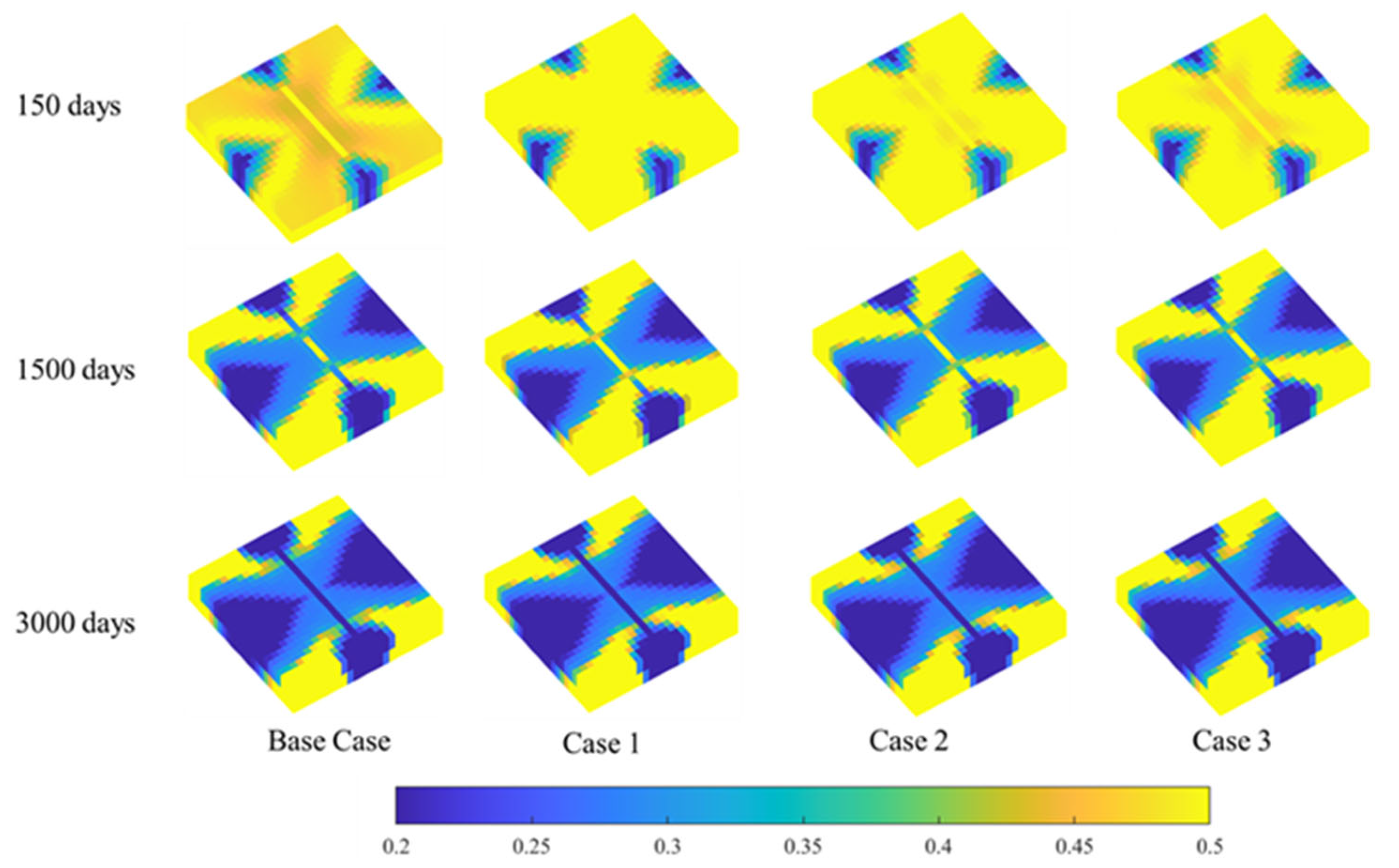
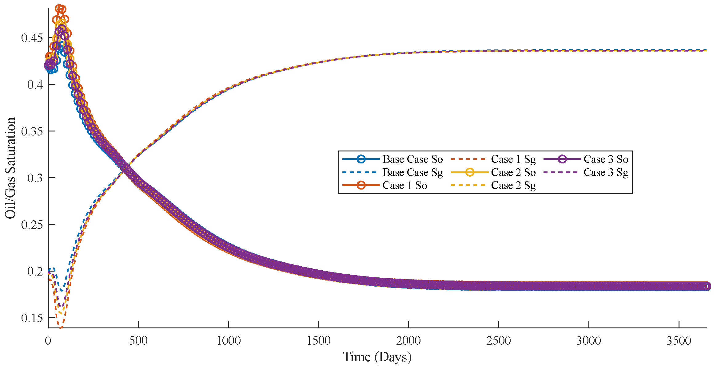
3.2.2. Key Findings on the Impact of Capillary Forces on Tight Oil Production
4. Conclusions
- Phase behavior in tight oil reservoirs is influenced by pore size and capillary forces, which traditional equations of state fail to capture in nanopores. This paper introduces capillary forces into traditional equations of state and compositional numerical simulations, improving phase equilibrium calculations using MRST.
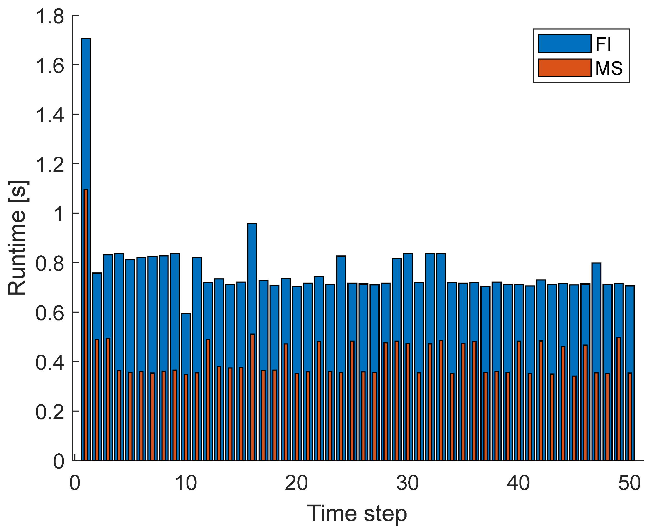
- To enhance iterative solution efficiency, a sequential solution format is employed, leveraging the parallel advantages of the improved multiscale finite volume method for pressure equation resolution. Numerical validation with a one-dimensional model confirms that this method enhances solution efficiency without compromising accuracy.
- Using the proposed multiscale compositional simulation method, the impact of capillary forces on phase equilibrium and tight oil recovery is analyzed. Sensitivity analysis shows that smaller pore radii lead to more pronounced capillary effects, with a decrease in bubble point and dew point lines, and an increase in calculation iterations. For tight oil recovery, capillary forces generally result in higher cumulative oil production and improved recovery rates for heavy components. Capillary effects lower bubble point pressure, suppress gas stripping and increase oil saturation while decreasing gas saturation.
- Compared to traditional numerical simulators, the proposed multiscale compositional method, which accounts for capillary forces, better characterizes phase behavior in tight oil reservoirs. This approach is significant for PVT simulation, development of numerical simulations, and forecasting development strategies in tight oil reservoirs.
Author Contributions
Funding
Institutional Review Board Statement
Informed Consent Statement
Data Availability Statement
Acknowledgments
Conflicts of Interest
References
- Zhu, W.; Yue, M.; Liu, Y.; Liu, K.; Song, Z. Research Progress on the Development Theory of Tight Oil Reservoirs in China. Chin. J. Eng. 2019, 41, 1103–1114. [Google Scholar] [CrossRef]
- Zhu, R.; Zou, C.; Wu, S.; Yang, Z.; Mao, Z.; Yang, H.; Fan, C.; Hui, X.; Cui, J.; Su, L.; et al. Formation Mechanism and Enrichment Patterns of Continental Tight Oil in China. Oil Gas Geol. 2019, 40, 1168–1184. [Google Scholar]
- Sun, L.; Zou, C.; Jia, A.; Wei, Y.; Zhu, R.; Wu, S.; Guo, Z. Characteristics and Development Trends of China’s Tight Oil and Gas. Pet. Explor. Dev. 2019, 46, 1015–1026. [Google Scholar] [CrossRef]
- Lee, E.Y.; Fathy, D.; Xiang, X.; Spahić, D.; Ahmed, M.S.; Fathi, E.; Sami, M. Middle Miocene syn-rift sequence on the central Gulf of Suez, Egypt: Depositional environment, diagenesis, and their roles in reservoir quality. Mar. Pet. Geol. 2025, 174, 107305. [Google Scholar] [CrossRef]
- Jia, C.; Zheng, M.; Zhang, Y. Unconventional hydrocarbon resources in China and the prospect of exploration and development. Pet. Explor. Dev. 2012, 39, 139–146. [Google Scholar] [CrossRef]
- Li, J.; Zheng, M.; Zhang, G.; Yang, T.; Wang, S.; Dong, D.; Wu, X.; Qu, H.; Chen, X. Potential and prospects of conventional and unconventional natural gas resource in China. Acta Pet. Sin. 2012, 33, 89–98. [Google Scholar]
- Loucks, R.G.; Reed, R.M.; Ruppel, S.C.; Jarvie, D.M. Morphology, Genesis, and Distribution of Nanometer-Scale Pores in Siliceous Mudstones of the Mississippian Barnett Shale. J. Sediment. Res. 2009, 79, 848–861. [Google Scholar] [CrossRef]
- Sigal, R.F. Pore-Size Distributions for Organic-Shale-Reservoir Rocks From Nuclear-Magnetic-Resonance Spectra Combined With Adsorption Measurements. SPE J. 2015, 20, 824–830. [Google Scholar] [CrossRef]
- Shi, W.; Liu, X.; Gao, M.; Tao, L.; Bai, J.; Zhu, Q. Pressuredrop Response Characteristics for Multi-Injection Well Interfered Vertical Well in Heterogeneous Fractured Anticline Reservoirs. J. Energy Resour. Technol. 2023, 145, 092902. [Google Scholar] [CrossRef]
- Jing, W.; Zhang, L.; Zhang, Y.; Memon, B.S.; Li, A.; Zhong, J.; Sun, H.; Yang, Y.; Cheng, Y.; Yao, J. Phase behavior of gas condensate in fractured-vuggy porous media based on microfluidic technology and real-time computed tomography scanning. Phys. Fluids 2023, 35, 122002. [Google Scholar] [CrossRef]
- Zuo, M.; Chen, H.; Qi, X.; Liu, X.; Xu, C.; Yu, H.; Brahim, M.S.; Wu, Y.C.; Liu, H. Effects of CO2 injection volume and formation of in-situ new phase on oil phase behavior during CO2 injection for enhanced oil recovery (EOR) in tight oil reservoirs. Chem. Eng. J. 2022, 452, 139454. [Google Scholar] [CrossRef]
- Peng, D.-Y.; Robinson, D.B. A New Two-Constant Equation of State. Ind. Eng. Chem. Fundam. 1976, 15, 59–64. [Google Scholar] [CrossRef]
- Melhem, G.A.; Saini, R.; Goodwin, B.M. A modified Peng-Robinson equation of state. Fluid Phase Equilibria 1989, 47, 189–237. [Google Scholar] [CrossRef]
- Stryjek, R.; Vera, J.H. PRSV—An improved Peng-Robinson equation of state with new mixing rules for strongly nonideal mixtures. Can. J. Chem. Eng. 1986, 64, 334–340. [Google Scholar] [CrossRef]
- Hu, J.; Du, C. Phase Behavior Study in Petroleum Systems. Inn. Mong. Petrochem. 2005, 87–88. [Google Scholar]
- Barsotti, E.; Tan, S.P.; Saraji, S.; Piri, M.; Chen, J.-H. A review on capillary condensation in nanoporous media: Implications for hydrocarbon recovery from tight reservoirs. Fuel 2016, 184, 344–361. [Google Scholar] [CrossRef]
- Jin, Z.; Firoozabadi, A. Thermodynamic Modeling of Phase Behavior in Shale Media. SPE J. 2016, 21, 190–207. [Google Scholar] [CrossRef]
- Sun, H.; Li, H.A. A New Three-Phase Flash Algorithm Considering Capillary Pressure in a Confined Space. Chem. Eng. Sci. 2019, 193, 346–363. [Google Scholar] [CrossRef]
- Ribeiro Carrott, M.M.L.; Candeias, A.J.E.; Carrott, P.J.M.; Ravikovitch, P.I.; Neimark, A.V.; Sequeira, A.D. Adsorption of nitrogen, neopentane, n-hexane, benzene and methanol for the evaluation of pore sizes in silica grades of MCM-41. Microporous Mesoporous Mater. 2001, 47, 323–337. [Google Scholar] [CrossRef]
- Qiao, S.Z.; Bhatia, S.K.; Nicholson, D. Study of Hexane Adsorption in Nanoporous MCM-41 Silica. Langmuir 2004, 20, 389–395. [Google Scholar] [CrossRef]
- Morishige, K.; Kawano, K.; Hayashigi, T. Adsorption Isotherm and Freezing of Kr in a Single Cylindrical Pore. J. Phys. Chem. B 2000, 104, 10298–10303. [Google Scholar] [CrossRef]
- Russo, P.A.; Carrott, M.M.L.R.; Carrott, P.J.M. Hydrocarbons adsorption on templated mesoporous materials: Effect of the pore size, geometry and surface chemistry. New J. Chem. 2011, 35, 407–416. [Google Scholar] [CrossRef]
- Yun, J.-H.; Düren, T.; Keil, F.J.; Seaton, N.A. Adsorption of Methane, Ethane, and Their Binary Mixtures on MCM-41: Experimental Evaluation of Methods for the Prediction of Adsorption Equilibrium. Langmuir 2002, 18, 2693–2701. [Google Scholar] [CrossRef]
- Zeigermann, P.; Dvoyashkin, M.; Valiullin, R.; Kärger, J. Assessing the pore critical point of the confined fluid by diffusion measurement. Diffus. Fundam. 2009, 41, 1–2. [Google Scholar] [CrossRef]
- Ally, J.; Molla, S.; Mostowfi, F. Condensation in Nanoporous Packed Beds. Langmuir 2016, 32, 4494–4499. [Google Scholar] [CrossRef]
- Alfi, M.; Nasrabadi, H.; Banerjee, D. Experimental investigation of confinement effect on phase behavior of hexane, heptane and octane using lab-on-a-chip technology. Fluid Phase Equilibria 2016, 423, 25–33. [Google Scholar] [CrossRef]
- Zhong, J.; Riordon, J.; Zandavi, S.H.; Xu, Y.; Persad, A.H.; Mostowfi, F.; Sinton, D. Capillary Condensation in 8 nm Deep Channels. J. Phys. Chem. Lett. 2018, 9, 497–503. [Google Scholar] [CrossRef]
- Brusilovsky, A.I. Mathematical Simulation of Phase Behavior of Natural Multicomponent Systems at High Pressures With an Equation of State. SPE Reserv. Eng. 1992, 7, 117–122. [Google Scholar] [CrossRef]
- Pang, J.; Zuo, J.Y.; Zhang, D.; Du, L. Impact of Porous Media on Saturation Pressures of Gas and Oil in Tight Reservoirs. In Proceedings of the SPE Canadian Unconventional Resources Conference, Calgary, AB, Canada, 30 October–1 November 2012. [Google Scholar]
- Teklu, T.W.; Alharthy, N.; Kazemi, H.; Yin, X.; Graves, R.M.; AlSumaiti, A.M. Phase Behavior and Minimum Miscibility Pressure in Nanopores. Spe Reserv. Eval. Eng. 2014, 17, 396–403. [Google Scholar] [CrossRef]
- Qi, Z.; Liang, B.; Deng, R.; Du, Z.; Wang, S.; Zhao, W. Phase Behavior Study in the Deep Gas-Condensate Reservoir with Low Permeability. In Proceedings of the EUROPEC/EAGE Conference and Exhibition, London, UK, 11–14 June 2007. [Google Scholar]
- Nojabaei, B.; Johns, R.T.; Chu, L. Effect of Capillary Pressure on Phase Behavior in Tight Rocks and Shales. SPE Reserv. Eval. Eng. 2013, 16, 281–289. [Google Scholar] [CrossRef]
- Yuan, Z.; Yuan, D.; Yun, Z.; Dongli, Z. The Impact of Capillary Force Effects in Nanopores on the Productivity of Tight Oil Reservoirs. J. Zhejiang Univ. Sci. Technol. 2017, 29, 328–333. [Google Scholar]
- Li, Y.; Li, X.; Teng, S.; Xu, D. Equilibrium Calculation Considering the Interaction between Pore-Throats and Fluid Molecules, as well as Capillary Forces. Acta Pet. Sin. 2015, 36, 511–515. [Google Scholar]
- Zhang, Y.; Di, Y.; Liu, P.; Li, W. Simulation of tight fluid flow with the consideration of capillarity and stress-change effect. Sci. Rep. 2019, 9, 5324. [Google Scholar] [CrossRef]
- Wang, Y.; Yan, B.; Killough, J. Compositional Modeling of Tight Oil Using Dynamic Nanopore Properties. In Proceedings of the SPE Annual Technical Conference and Exhibition, New Orleans, LA, USA, 30 September–2 October 2013. [Google Scholar]
- Khoshghadam, M.; Khanal, A.; Rabinejadganji, N.; Lee, W.J. How to Model and Improve Our Understanding of Liquid-Rich Shale Reservoirs with Complex Organic/Inorganic Pore Network. In Proceedings of the SPE/AAPG/SEG Unconventional Resources Technology Conference, San Antonio, TX, USA, 1–3 August 2016. [Google Scholar]
- Yan, B.; Wang, Y.; Killough, J.E. A fully compositional model considering the effect of nanopores in tight oil reservoirs. J. Pet. Sci. Eng. 2017, 152, 675–682. [Google Scholar] [CrossRef]
- Zhang, Y.; Di, Y.; Yu, W.; Sepehrnoori, K. A Comprehensive Model for Investigation of Carbon Dioxide Enhanced Oil Recovery With Nanopore Confinement in the Bakken Tight Oil Reservoir. SPE Reserv. Eval. Eng. 2018, 22, 122–136. [Google Scholar] [CrossRef]
- Hou, T.Y.; Wu, X.-h. A Multiscale Finite Element Method for Elliptic Problems in Composite Materials and Porous Media. J. Comput. Phys. 1997, 134, 169–189. [Google Scholar] [CrossRef]
- Babuska, I.; Osborn, J.E. Generalized Finite Element Methods: Their Performance and Their Relation to Mixed Methods. SIAM J. Numer. Anal. 1983, 20, 510–536. [Google Scholar] [CrossRef]
- Jenny, P.; Lee, S.H.; Tchelepi, H.A. Multi-scale finite-volume method for elliptic problems in subsurface flow simulation. J. Comput. Phys. 2003, 187, 47–67. [Google Scholar] [CrossRef]
- Møyner, O.; Lie, K.-A. A Multiscale Restriction-Smoothed Basis Method for Compressible Black-Oil Models. SPE J. 2016, 21, 2079–2096. [Google Scholar] [CrossRef]
- Zhou, H.; Tchelepi, H.A.A. Two-Stage Algebraic Multiscale Linear Solver for Highly Heterogeneous Reservoir Models. SPE J. 2012, 17, 523–539. [Google Scholar] [CrossRef]
- Lunati, I.; Tyagi, M.; Lee, S.H. An iterative multiscale finite volume algorithm converging to the exact solution. J. Comput. Phys. 2011, 230, 1849–1864. [Google Scholar] [CrossRef]
- Møyner, O.; Lie, K.-A. A multiscale restriction-smoothed basis method for high contrast porous media represented on unstructured grids. J. Comput. Phys. 2016, 304, 46–71. [Google Scholar] [CrossRef]
- Wu, L.; Wang, J.; Jia, D.; Zhang, R.; Zhang, J.; Yan, Y.; Wang, S. A Multi-Scale Numerical Simulation Method Considering Anisotropic Relative Permeability. Processes 2024, 12, 2058. [Google Scholar] [CrossRef]
- Hu, X.; Hu, S.; Jin, F.; Huang, S. Physics of Petroleum Reservoirs; Springer: Berlin/Heidelberg, Germany, 2017. [Google Scholar] [CrossRef]
- Ma, Y. Study on the Phase Behavior of Nano-Pore Fluid and Numerical Simulation Method in Tight Reservoir. Ph.D. Thesis, China University of Geosciences, Beijing, China, 2023. [Google Scholar]
- Ferguson, A. On a relation between surface tension and density. Trans. Faraday Soc. 1923, 19, 407–412. [Google Scholar] [CrossRef]
- Pedersen, K.S.; Christensen, P.L.; Shaikh, J.A. Phase Behavior of Petroleum Reservoir Fluids; CRC Press: Boca Raton, FL, USA, 2006. [Google Scholar] [CrossRef]
- Riviere, B. Computational methods for multiphase flows in porous media. Math. Comput. 2007, 76, 2253–2255. [Google Scholar] [CrossRef]
- Peaceman, D.W. Interpretation of Well-Block Pressures in Numerical Reservoir Simulation(includes associated paper 6988). Soc. Pet. Eng. J. 1978, 18, 183–194. [Google Scholar] [CrossRef]
- Coats, K.H. A Note on IMPES and Some IMPES-Based Simulation Models. SPE J. 2000, 5, 245–251. [Google Scholar] [CrossRef]
- Møyner, O.; Tchelepi, H.A. A Mass-Conservative Sequential Implicit Multiscale Method for Isothermal Equation-of-State Compositional Problems. SPE J. 2018, 23, 2376–2393. [Google Scholar] [CrossRef]
- Wang, Y.; Hajibeygi, H.; Tchelepi, H.A. Algebraic multiscale solver for flow in heterogeneous porous media. J. Comput. Phys. 2014, 259, 284–303. [Google Scholar] [CrossRef]
- Møyner, O. Construction of Multiscale Preconditioners on Stratigraphic Grids. In Proceedings of the CMOR XIV—14th European Conference on the Mathematics of Oil Recovery Catania, Sicily, Italy, 8–11 September 2014. [Google Scholar]
- Lie, K.-A. An Introduction to Reservoir Simulation Using MATLAB/GNU Octave: User Guide for the MATLAB Reservoir Simulation Toolbox (MRST); Cambridge University Press: Cambridge, UK, 2019. [Google Scholar]
- Killough, J.E.; Kossack, C.A. Fifth Comparative Solution Project: Evaluation of Miscible Flood Simulators. In Proceedings of the SPE Symposium on Reservoir Simulation, San Antonio, TX, USA, 1–4 February 1987. [Google Scholar]
- Mallison, B.T.; Gerritsen, M.G.; Jessen, K.; Orr, F.M. High-Order Upwind Schemes for Two-Phase, Multicomponent Flow. SPE J. 2005, 10, 297–311. [Google Scholar] [CrossRef]


| Model Grid | Grid Size (m) | Initial Reservoir Temperature (°C) | Initial Reservoir Pressure (MPa) | Porosity (%) | Permeability (mD) | Injection Pressure (MPa) | Production Pressure (MPa) | Simulation Time (Year) |
|---|---|---|---|---|---|---|---|---|
| 1000 × 1 × 1 (coarse grid 100 × 1 × 1) | 1 × 1 × 0.1 | 150 | 7.5 | 25 | 10 | 10 | 5 | 20 |
| Component | Pc (Bar) | Tc (K) | Vc (L/mol) | Mol. Weight | Acentric Fact | Initial Total Composition Values |
|---|---|---|---|---|---|---|
| C1 | 45.922 | 190.654 | 0.09863 | 16.04 | 0.01142 | 0.3 |
| C10 | 21.03 | 617.7 | 0.6098 | 142.28 | 0.4884 | 0.6 |
| CO2 | 73.733 | 304.128 | 0.09412 | 44 | 0.22394 | 0.1 |
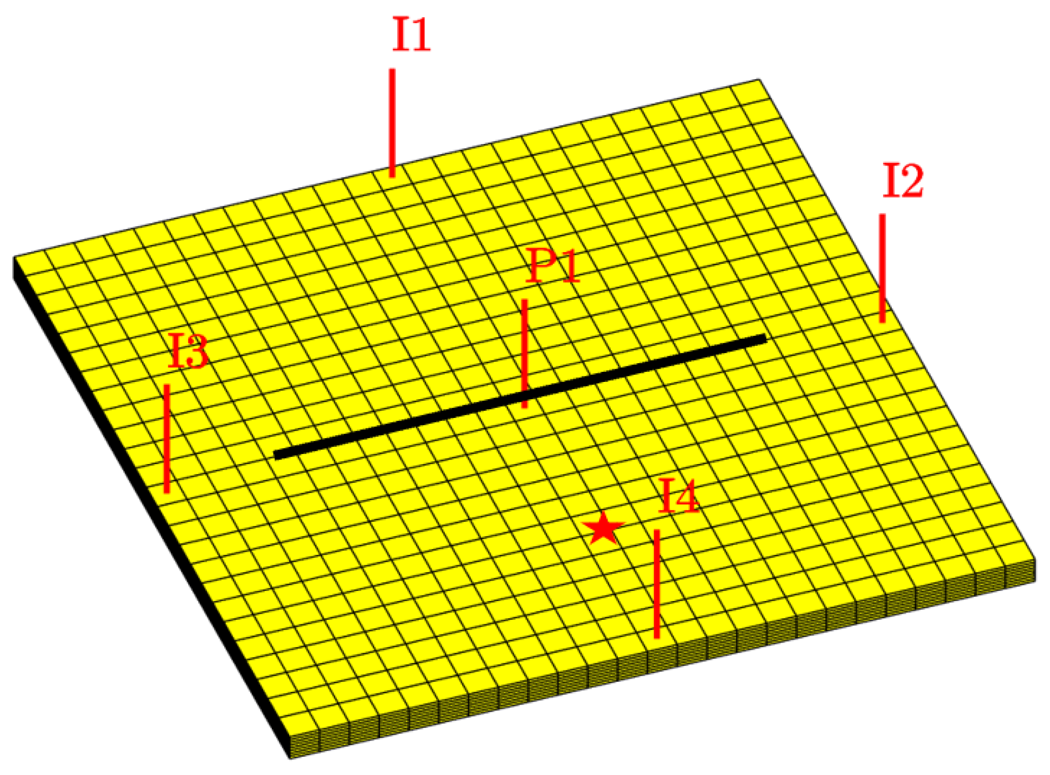
| Model Grid | Grid Size (m) | Initial Reservoir Temperature (°C) | Initial Reservoir Pressure (MPa) | Porosity (%) | Matrix Permeability (mD) | Fracture Permeability (mD) | Initial Saturation (Water, Oil, and Gas) (f) | The Bottom-Hole Pressure of the Producing Well (MPa) | The Daily Gas Injection Volume of an Injection Well (m3/day) |
|---|---|---|---|---|---|---|---|---|---|
| 25 × 25 × 8 | 40 × 40 × 5 | 114 | 15 | 8 | 10 | 1000 | 0.38, 0.62, 0 | 10 | 300 |
| Component | Pc (Bar) | Tc (K) | Vc (L/mol) | Mol. Weight | Acentric Fact | Initial Total Composition Values |
|---|---|---|---|---|---|---|
| N2/CH4 | 45.8 | 189.5 | 0.0997 | 16.1594 | 0.01142 | 0.463 |
| CO2 | 73.733 | 304.128 | 0.09412 | 44 | 0.22394 | 0.0164 |
| C2–5 | 41.0 | 387.6 | 0.02171 | 45.5725 | 0.167 | 0.2052 |
| C6–13 | 33.5 | 597.5 | 0.03812 | 11.774 | 0.386 | 0.19108 |
| C14–24 | 17.7 | 698.5 | 0.07214 | 24.8827 | 0.808 | 0.08113 |
| C25–80 | 11.7 | 875.0 | 0.01136 | 48.125 | 1.231 | 0.04319 |
Disclaimer/Publisher’s Note: The statements, opinions and data contained in all publications are solely those of the individual author(s) and contributor(s) and not of MDPI and/or the editor(s). MDPI and/or the editor(s) disclaim responsibility for any injury to people or property resulting from any ideas, methods, instructions or products referred to in the content. |
© 2025 by the authors. Licensee MDPI, Basel, Switzerland. This article is an open access article distributed under the terms and conditions of the Creative Commons Attribution (CC BY) license (https://creativecommons.org/licenses/by/4.0/).
Share and Cite
Wang, J.; Wu, L.; Sun, Q.; Zhang, R.; Chen, W.; Yang, H.; Wang, S. A Multiscale Compositional Numerical Study in Tight Oil Reservoir: Incorporating Capillary Forces in Phase Behavior Calculation. Appl. Sci. 2025, 15, 3082. https://doi.org/10.3390/app15063082
Wang J, Wu L, Sun Q, Zhang R, Chen W, Yang H, Wang S. A Multiscale Compositional Numerical Study in Tight Oil Reservoir: Incorporating Capillary Forces in Phase Behavior Calculation. Applied Sciences. 2025; 15(6):3082. https://doi.org/10.3390/app15063082
Chicago/Turabian StyleWang, Junqiang, Li Wu, Qian Sun, Ruichao Zhang, Wenbin Chen, Haitong Yang, and Shuoliang Wang. 2025. "A Multiscale Compositional Numerical Study in Tight Oil Reservoir: Incorporating Capillary Forces in Phase Behavior Calculation" Applied Sciences 15, no. 6: 3082. https://doi.org/10.3390/app15063082
APA StyleWang, J., Wu, L., Sun, Q., Zhang, R., Chen, W., Yang, H., & Wang, S. (2025). A Multiscale Compositional Numerical Study in Tight Oil Reservoir: Incorporating Capillary Forces in Phase Behavior Calculation. Applied Sciences, 15(6), 3082. https://doi.org/10.3390/app15063082