Article

Concept Drift Detection Based on Deep Neural Networks and Autoencoders

School of Management Science and Information Engineering, Hebei University of Economics and Business, Shijiazhuang 050061, China
*
Author to whom correspondence should be addressed.
Appl. Sci. 2025, 15(6), 3056; https://doi.org/10.3390/app15063056
Submission received: 22 January 2025 / Revised: 28 February 2025 / Accepted: 7 March 2025 / Published: 12 March 2025

Abstract

:
In domains such as fraud detection, healthcare, and industrial equipment maintenance, streaming data often exhibit characteristics such as continuous generation, high real-time processing requirements, and complex distributions, making it susceptible to concept drift. Traditional shallow models, with their limited representational capacity, struggle to fully capture the latent conceptual knowledge inherent in the dynamic and evolving nature of streaming data. To address this challenge, we propose a concept drift detection method based on deep neural networks combined with autoencoders (Concept Drift Detection Based on Deep Neural Network Combined with Autoencoder, DNN+AE-DD). In the DNN+AE-DD, a deep neural network is first employed as the base model for pretraining, and the hidden layer parameters of the model are transferred to a network with an identical structure for stream data processing, where certain hidden layers are frozen. Subsequently, the hidden layer outputs from both the pretraining and stream data processing phases are collected and used as training and testing data to initialize and predict using an autoencoder model. Concept drift is then detected by combining the reconstruction error of the autoencoder with the 3 σ principle. Experimental results on both real-world and synthetic datasets demonstrate that, compared to traditional shallow concept drift detection methods, this approach effectively and accurately detects anomalies in streaming data, confirming the proposed model’s high sensitivity to concept drift.

1. Introduction

In the era of big data, the exponential growth of information generated from sources such as social media [1,2], online transactions [3,4], and credit card fraud [5,6] results in the continuous production of vast amounts of data, commonly referred to as data streams. Unlike traditional static data, data streams are characterized by their infinite and dynamic nature, which not only presents significant challenges for conventional model training and learning but also introduces a critical issue—concept drift [7].
Assuming that a data stream follows a specific distribution, concept drift refers to a change in this distribution over time, causing the data stream to follow different distributions at different time points. If, at time t, the data follow distribution D t ( x , y ) and, at time t + 1 , the data stream follows distribution D t + 1 ( x , y ) , concept drift [8] is said to occur at time t + 1 , if D t ( x , y ) D t + 1 ( x , y ) . The occurrence of concept drift typically leads to a significant decline in performance metrics, such as classification accuracy and precision, for the current model in the short term, making the model unsuitable for the post-drift data stream. Therefore, when processing data streams, it is essential to account for the potential issue of concept drift.
Currently, approaches for handling concept drift can be categorized into two main types: concept drift detection and concept drift adaptation [9]. The objective of concept drift adaptation is to enhance the model’s ability to adjust to changing data. For streaming data, regardless of whether drift occurs, the focus is on the passive adjustment and adaptation of the model to the current data. This involves improving the model’s generalization and representation capabilities for the current data. In contrast, concept drift detection takes a proactive approach, aiming primarily to identify whether concept drift has occurred in the data stream. The focus of drift detection is on identifying the time points, duration, and other characteristics of the drift, i.e., determining whether concept drift has occurred at each moment in time. Concept drift detection and adaptation are not mutually exclusive. When the model’s drift detection is accurate, it can assist adaptation by further enhancing the model’s representation capabilities and robustness. Moreover, timely detection can prevent unnecessary updates to the model, saving time and improving its efficiency in handling concept drift in streaming data. This leads to a more effective and responsive system for managing concept drift. Consequently, the primary focus of this paper is on concept drift detection.
Effective concept drift detection methods have significant applications in areas such as fraud detection, disease monitoring, and industrial equipment maintenance. In fraud detection, concept drift detection methods enable fraud detection models to identify and adapt to emerging fraud patterns, thereby mitigating the negative consequences of fraudulent activities. In disease monitoring, patients’ physical conditions may change as treatment progresses or the disease advances. Concept drift detection methods aid in capturing these physiological and pathological changes in a timely manner, enabling doctors to detect and intervene early, while also adjusting treatment plans in real time. In the Municipal Solid Waste Incineration (MSWI) process [10], harmful gases such as dioxins may be generated due to factors such as industrial environments or equipment wear. This necessitates the monitoring of parameters like temperature and humidity during the MSWI process. Concept drift detection models can facilitate the real-time and accurate measurement of these parameters, thereby reducing harmful gas emissions.
Various concept drift detection methods have been proposed by scholars, including the drift detection method (DDM) [11], the Adaptive Sliding Window (ADWIN) [12], concept drift detection methods based on online performance tests (CDPTs) [13], a K-Means clustering- and SVM-based hybrid concept drift detection technique for network anomaly detection [14], and a semi-supervised concept drift detection method by combining sample output space and feature space with its application [10], among others. Most of these methods are based on traditional machine learning techniques, such as Support Vector Machines (SVM), Principal Component Analysis (PCA), Naive Bayes, and Hoeffding Trees. However, traditional machine learning methods rely on feature extraction processes to handle data, which inherently limits their representational capacity and restricts them to shallow learning. In contrast, deep learning employs multi-layer neural networks to autonomously learn the deep features of data, enabling it to handle more complex datasets and nonlinear problems, thus offering superior learning capabilities. While a limited number of studies have explored deep network models, the application of deep learning to concept drift detection is still in its infancy and requires further systematic investigation.
Based on this, this paper proposes a concept drift detection method, termed DNN+AE-DD, which integrates a deep neural network model with an autoencoder. In this approach, a deep neural network serves as the base classifier for model training. A structurally identical neural network is employed for processing streaming data, with certain network weights frozen to preserve learned representations. Finally, the method leverages autoencoders and the 3 σ principle to detect concept drift by analyzing the outputs of the model’s hidden layers.The contributions of this paper are as follows:
  • Propose a new drift detection framework.
  • Apply autoencoders combined with the 3 σ principle for concept drift detection.
  • Validate the ideas presented in this paper using both synthetic and real-world data. The results demonstrate that the model proposed in this paper performs excellently based on the evaluation metrics and datasets used.
The structure of this paper is organized as follows: Section 2 offers a concise review of drift detection methods developed by various researchers in recent years to address the challenge of concept drift. Section 3 provides a comprehensive description of the proposed method. Section 4 presents and analyzes the experimental results. Finally, Section 5 concludes the paper and outlines potential directions for future research.

2. Related Work

Concept drift can be roughly classified into four types based on different drift characteristics [15]: sudden drift, gradual drift, incremental drift, and reoccurring drift, as illustrated in Figure 1 (The blue line represents the distribution of the old concept to which the data belongs, the red line indicates the distribution of the new concept, and the black line depicts the transition from the old concept distribution to the new concept distribution). Relevant studies typically focus on detecting some or all of these drift types. For instance, the Active Drift Detection based on Meta learning (Meta-ADD) [16] detects sudden, gradual, and incremental drifts. The LSTM Drift Detector (LSTMDD) [17] is designed to detect sudden and gradual drifts. The Weakly Supervised Conceptual Drift Detection method based on the Online Deep Neural Network (WSCDD) [18] is capable of detecting all four types of concept drift.
Currently, several methods for detecting concept drift have been proposed. This paper categorizes these existing detection methods into two groups based on the models employed: concept drift detection methods that rely on traditional machine learning models and those that utilize deep learning models.

2.1. Concept Drift Detection Methods Based on Traditional Machine Learning Approaches

Concept drift detection based on traditional machine learning models can be divided into three categories [19]: error rate-based concept drift detection methods, data distribution-based concept drift detection methods, and hypothesis testing-based concept drift detection methods.
The drift detection method (DDM) is a representative approach for concept drift detection based on error rates. It determines a threshold by calculating the minimum error rate and standard deviation during the training process of the data stream. The current error rate and standard deviation are then compared with this threshold to assess whether a drift condition has occurred. While DDM demonstrates good generalization ability, it is less effective in detecting gradual concept drift. The early drift detection method (EDDM) [20] improves upon DDM’s drift detection criteria, enhancing the detector’s sensitivity to gradual drift, thereby making it more suitable for detecting gradual changes. The drift detection method based on Hoeffding’s inequality with the A -test (HDDM_A) [21] is an extension of DDM that incorporates Hoeffding’s inequality, while the W -test on HDDM (HDDM_W) [21] applies McDiarmid’s bounds. The ADWIN algorithm, a notable representative of concept drift detection using a sliding window, adaptively partitions two windows according to specific rules and computes the difference in certain statistical values within these windows. If the difference exceeds a predefined threshold, drift is detected. Compared to other methods, ADWIN demonstrates superior robustness and does not require prior knowledge of the data.
The essence of concept drift lies in changes in the data distribution. Data distribution-based concept drift detection methods focus on measuring these changes, with variations in research methodologies primarily driven by the choice of different distance metrics. KSWIN [22] combines a sliding window approach with the Kolmogorov–Smirnov (K-S) test to detect drift by assessing the distribution differences between two windows. The concept drift detection method (CDDD) [23] introduces an innovative approach by collecting and storing data feature information either from previous drift detections or from the beginning of the data stream.
Hypothesis testing-based concept drift detection methods leverage various hypothesis testing techniques to identify concept drift. De Lima Cabral et al. [24] introduced the Fisher Exact Test for concept drift detection, while Han et al. [25] employed the Kolmogorov–Smirnov (K-S) test for the same purpose.

2.2. Concept Drift Detection Methods Based on Deep Learning Models

Some studies have applied deep learning techniques to address the challenge of concept drift. As a rapidly advancing technology, deep learning has become the focal point of research and application across various domains, demonstrating significant maturity in areas such as image recognition, speech recognition, and natural language processing. Compared to traditional machine learning methods, deep learning offers enhanced representational and fitting capabilities, making it well suited for handling complex data stream scenarios. Based on the classification of deep neural networks according to their network structures, deep learning models can be divided into three types: feedforward networks, memory networks, and graph networks [26]. Building on this classification, this paper categorizes deep learning-based concept drift detection methods into three groups: those based on feedforward networks, memory networks, and graph networks.
Meta-ADD [16] utilizes drift data for offline pretraining to extract meta-features associated with error rates, employing prototype networks to identify different categories of concept drift. It can detect drift types without the need for pre-specified hypothesis testing. However, it lacks pretraining and suffers from a cold start problem [9]. CIDD-ADODNN [27] classifies imbalanced data streams using a deep neural network optimized with Adadelta and subsequently applies the ADWIN algorithm to detect concept drift. By incorporating techniques to address class imbalance, it effectively handles the challenges associated with imbalanced streaming data. WSCDD [18] trains neural network models using the Hedge backpropagation algorithm, while employing Monte Carlo methods to calculate prediction uncertainty. This uncertainty is then used as input for the ADWIN algorithm to detect concept drift. Given the difficulty of obtaining labeled data in weakly supervised environments, WSCDD can detect the occurrence of concept drift in unlabeled data. The concept drift detection model based on Bidirectional Temporal Convolutional Networks and Multi-Stacking Ensemble Learning (CD-BTMSE) [28] leverages a Bidirectional Temporal Convolutional Network (BiTCN) and a multi-stacking ensemble learning model to improve the generalization ability and accuracy of drift detection, while simultaneously addressing the issue of class imbalance. By incorporating the BiTCN model, it enhances the model’s performance on time series data, an area where traditional models typically underperform, thereby overcoming the limitations of existing ensemble methods. In response to the scarcity and high acquisition costs of true labels, the Uncertainty Drift Detection (UDD) [29] algorithm combines the uncertainty provided by deep neural networks with Monte Carlo Dropout. It detects temporal structural changes using the ADWIN algorithm and retrains the model when drift is detected.
SDLS [30] combines long short-term memory (LSTM) networks with a sliding window approach to predict data, selecting an appropriate window size to analyze prediction differences. It models all values within the window and assigns anomaly scores based on the probability density of these differences, thereby enabling concept drift detection. Hatamikhah et al. [31] utilize the Stream Ensemble SEA algorithm, incorporating deep belief networks as the foundational model. The LSTM Drift Detector (LSTMDD) [17] proposes an attention-enhanced LSTM model, integrated with a genetic hyper-tuning drift detector, to effectively detect concept drift in non-Gaussian distributed cloud computing environments.
Lin et al. [32] propose the use of graph convolutional networks (GCNs) for concept drift detection. This method first converts log trajectories into activity graphs, and then applies GCNs to learn from these graphs and construct virtual nodes. Drift is assessed based on the distances between these virtual nodes. Compared to other business process detection methods, this approach leverages deep models to autonomously define monitoring features and focuses specifically on detecting abrupt concept drift within the business process. The Graph Convolutional Network for Drift Detection (GDD) [33] transforms event sequences into directed and sequential graphs. It utilizes GCNs to extract features and introduces virtual nodes to represent potential features. The distances between these virtual nodes are calculated, and the K-means algorithm is applied to identify outliers among candidate change points. A filtering mechanism is then employed to confirm the actual change points, allowing GDDs to autonomously capture evolving features while maintaining reasonable performance levels.
Currently, there is limited research on applying deep learning to address concept drift, likely due to the fact that deep learning models typically require more computational resources and time. Under the same computational resources, deep learning models tend to have slower processing times compared to traditional shallow models with simpler architectures, and excessive delays can hinder the effectiveness of drift detection [34]. There are several challenges in using deep learning techniques to handle concept drift: the online learning scenario of streaming data demands models with flexible structures, capable of adjusting their capacity at different stages of the data stream. However, neural network models with different layers exhibit varying convergence speeds, resulting in data of different sizes and complexities being suitable for processing. If the model is shallow, it may suffer from insufficient representational power, limiting its ability to address complex nonlinear problems. Conversely, deeper models often struggle with slow convergence speeds. Additionally, typical issues in deep neural networks, such as vanishing gradients and reduced feature reuse, can also impair the classifier’s ability to adapt to new concepts [35]. As a result, while previous studies have explored deep learning for concept drift detection, this area remains in its early stages, with significant untapped potential. Therefore, this paper proposes a concept drift detection method based on deep neural networks and autoencoders, aiming to contribute to this emerging field of research.

3. Methodology

The framework of this paper is shown in Figure 2. Firstly, static data D is used to train Model1, obtaining the outputs of Model1 a ( L ) as training data to be passed to Model3. After training is completed, the trained weights W , b are transferred to Model2, which is initialized with those weights. Then, the merged Model2 processes the stream data S to obtain a weight list o ( L ) , which is passed as test data to Model3. Model3 uses the previously obtained training data a ( L ) to train the model, calculate the training error e a , and compute a threshold as the basis for the 3 σ judgment criterion. Finally, the loss e s obtained from the test dataset o ( L ) is combined with the 3 σ criterion to determine the occurrence of concept drift. For the DNN+AE-DD drift detection model, Model1 and Model2 are implemented using DNN networks, while Model3 is implemented using an autoencoder. Algorithm 1 outlines the overall process of the DNN+AE-DD.
This section divides the work of this paper into three stages. Section 3.1 provides a detailed explanation of the pretraining process, including the model’s inputs and outputs during training. The handling of stream data and the process of weight replication are discussed in Section 3.2. Finally, Section 3.3 focuses on the core contribution of this paper: the use of autoencoders in conjunction with the 3 σ principle for anomaly detection.
Algorithm 1 DNN+AE-DD operational workflow
Input: Non-drift data D = { ( x 1 , y 1 ) , ( x 2 , y 2 ) , , ( x m , y m ) } , Stream data S = { ( x 1 , y 1 ) , ( x 2 , y 2 ) , ( x 3 , y 3 ) , , ( x t , y t ) , } .
Output: Drift position.
1:
Processing non-drift data D with Model1 according to Algorithm 2 and generate train data a ( L ) .
2:
Utilize stream data S and weights W, b from Model1 to initialize the Model2 according to the Algorithm 3 and generate test data o ( L ) .
3:
Utilize the train data a ( L ) from Model1 to train Model3 and obtain reconstruction error e a to provide threshold for 3 σ rules.
4:
Utilize the test data o ( L ) from Model2 and obtain reconstruction error e s integrate 3 σ rules obtain drift position (to see the details in Algorithm 4).

3.1. Pretrain

This section focuses on the overall process of the pretraining stage, as shown in Figure 3 and Algorithm 2. First, a DNN model, referred to as Model1, is initialized (refer to statement 2 of Algorithm 2), and the model is trained using static data (non-drift data) D (refer to statements 3 through 8 of Algorithm 2) to obtain and save the outputs a ( L ) from the last hidden layer. Simultaneously, the connection weights W , b between all neurons in the hidden layers are collected and stored (indicated by the purple box in the figure). The final dimension of the obtained hidden layer outputs is a matrix formed by multiplying the number of neurons in the last hidden layer by the batch size, represented by the matrix composed of red neurons in Figure 3. We select the last 5000 sets of outputs from the saved last hidden layer (as shown in the yellow box in Figure 3) as training data for drift detection. Due to the time-intensive nature of the training process, we selected only a portion of the collected weights. Additionally, in the later stages of neural network training, the model is able to fit the data to a certain extent, with the hidden layer output partially representing the distribution of data under the old concept. Unlike streaming data, this output is static, generated from previous batch training using non-drift data.
Algorithm 2 Pretrain process
Input: Non-drift data D = { ( x 1 , y 1 ) , ( x 2 , y 2 ) , , ( x m , y m ) } , the number of layers L, the number of neurons per layer M F , M S , M L , the learning rate η 1 , the loss function L P , the optimizer o p t i m 1 , the delay rate γ 1 , the learning rate update step size s 1 , the iterations p r e t r a i n _ i t e r s .
Output: Last hidden outputs matrix a ( L ) = [ a 1 ( L ) , a 2 ( L ) , , a m ( L ) ] , weights and bias associated with all hidden layers W = [ W ( F ) , W ( S ) , , W ( L ) ] , b = [ b ( F ) , b ( S ) , , b ( L ) ] , F, S, L represent the number of layer, W ( I ) = [ w 1 ( I ) , w 2 ( I ) , , w m ( I ) ] , b ( I ) = [ b 1 ( I ) , b 2 ( I ) , , b m ( I ) ] .
1:
Processing data D with StandardScaler.
2:
Initialize weight matrix W with random values.
3:
for   e p o c h = 1   to   p r e t r a i n _ i t e r s   do
4:
   for  ( x i , y i )   inD do
5:
     Obtain the prediction y i ^ .
6:
     Calculate the loss L P ( y i , y i ^ ) between prediction y i ^ and true label y i .
7:
     Perform loss backward and update all the hidden layers’ parameters W, b.
8:
   end for
9:
end for

3.2. Processing Stream Data

The data stream processing flow is shown in Figure 4, and the algorithm is detailed in Algorithm 3. Model2 uses the same network structure as Model1. The difference lies in the model initialization, which is carried out as follows: the connection weights and biases, W , b , of all the hidden neurons in the trained Model1 are copied to Model2, and the parameters W ( F ) , W ( S ) , b ( F ) , b ( S ) (highlighted in the blue box in Figure 4) of all hidden layers, except for the last hidden layer, are frozen (see step 2 in Algorithm 2).This approach is based on the following considerations: first, neural networks have feature representation capabilities, and using pretrained model weights helps reduce the time required for retraining. Secondly, assuming that the hidden layer parameters of the trained model can represent data belonging to the old concept distribution, we copy and freeze the connection weights and biases of the earlier hidden layers to assist the model in recognizing data from the old concept distribution in the data stream. The last hidden layer is kept in an updatable state, allowing the model to adjust its parameters promptly when new concept distributions emerge in the data stream.
After the model initialization is completed, Model2 is used to process the data stream S (refer to steps 3-6 in Algorithm 3), and the output from the last hidden layer, o ( L ) , is collected as the test data for Model3.To demonstrate that the weights of the last hidden layer in Model2 exhibit significant differences before and after the drift in Figure 4, detailed analysis is provided in Appendix A. This test data are represented by the deep pink neurons within the green box in Figure 4. In contrast to the hidden layer output of Model1, the hidden layer output of Model2 corresponds to the output in the online learning scenario. Since the data stream requires the model to learn from one data point at a time and produce a corresponding output, the weights displayed in the figure reflect the data stream format, indicating that the processing of the data stream is conducted in an online setting.
Algorithm 3 Process stream data
Input: Stream data S = { ( x 1 , y 1 ) , ( x 2 , y 2 ) , ( x 3 , y 3 ) , , ( x t , y t ) , } , x i represent the feature of sample, y i represent the label, weights and bias associated with all hidden layers W, b obtained from pretrain, learning rate η 2 , the loss function L P , the optimizer o p t i m 1 , the delay rate γ 2 , the learning rate update step size s 2 .
Output: Last hidden layer’s output stream o ( L ) = [ o 1 ( L ) , o 2 ( L ) , , o t ( L ) , ] .
1:
Normalize the stream data S with StandardScaler.
2:
Initialize the DNN network with W, b and frozen the first two hidden layers neurons’ parameters W ( F ) , W ( S ) , b ( F ) , b ( S ) , keep the last hidden layer neuron’s weights W F ( L ) and bias b F ( L ) active.
3:
for  ( x k , y k )  in S do
4:
   Calculate the prediction value y k ^ .
5:
   Calculate the loss L P ( y k , y k ^ ) between prediction y k ^ and true label y k .
6:
   Loss backward and only update the parameters W F ( L ) , b F ( L ) of the active layer.
7:
end for

3.3. Concept Drift Detection

The detection process is depicted in Figure 5, with the corresponding algorithm detailed in Algorithm 4. In this work, we utilize an autoencoder (Model3) combined with the 3 σ principle for anomaly detection in streaming data. The 3 σ principle assumes that the data follow a normal distribution, where μ represents the mean and σ denotes the standard deviation. According to this principle, the probability of a value falling within the range ( μ 3 σ , μ + 3 σ ) is 0.9974. Consequently, values outside this range are considered anomalous and classified as drift data.We conducted experiments on the selection of different drift thresholds, with detailed results provided in Appendix A. During the drift detection phase, the 3 σ criterion serves as the threshold for identifying anomalies. Given the assumption of normality, over 99.7% of the data points should fall within this range, with outliers beyond it being flagged as anomalous.The autoencoder functions similarly to a sliding window when filtering the data. However, unlike traditional sliding windows, the autoencoder is more sensitive to changes in the underlying data distribution and does not require predefined window sizes or step lengths. Its role is analogous to that of a one-class classifier: by training the autoencoder on data from the old concept distribution, it learns to reconstruct data conforming to that distribution. Data from a new concept distribution, which the autoencoder has not encountered before, are more difficult to reconstruct, leading to reconstruction errors that differ from those of the old data. Concept drift is detected by analyzing the reconstruction errors of the streaming data, in conjunction with the 3 σ principle.
Using the last-layer hidden outputs, a ( L ) , of Model1 for the last 5000 samples (indicated as red neurons in the yellow box), Model3 is initialized (see Algorithm 4, lines 2–8). The reconstruction errors, e a , for the training data are then computed, along with the mean, μ , and standard deviation, σ , of all reconstruction errors. The upper and lower threshold limits are established based on the 3 σ principle. The overall process is illustrated by the red arrows in Figure 5, with the corresponding steps outlined in Algorithm 4 (lines 9–10). The formulas for calculating the mean, μ , and threshold limits are as follows:
μ = i = 1 5000 t r a i n _ r e c o n s t r u c t i o n _ e r r o r / 5000
l o w e r _ t h r e s h o l d = μ 3 σ
u p p e r _ t h r e s h o l d = μ + 3 σ
When the final hidden layer output o ( L ) (deep pink neuron—green box) from Model2 is received, it is used as test data to compute the reconstruction error e s (refer to the blue arrow in Figure 5). This error is then compared with the threshold limits derived from the 3 σ principle. Data points whose errors fall outside the threshold range are classified as drift data (refer to lines 11–16 of Algorithm 4). The reason for selecting the final hidden layer outputs of the model as both training and test data is as follows: Model2, initialized by copying and freezing the connection weights from Model1, is capable of distinguishing between data belonging to old and new concepts. Consequently, the model’s performance varies for data associated with different concepts, which is reflected in the model’s predictions. Since the weights in the model are influenced by error backpropagation during training, we reason that the output of the final hidden layer, being closest to the model’s prediction, will also manifest this distinction. Therefore, in both Model1 and Model2, we collect the outputs of the final hidden layer and use them separately as training and test data.
Algorithm 4 Concept drift detection
Input: The pretrain output matrix a ( L ) = [ a 1 ( L ) , a 2 ( L ) , , a m ( L ) ] , the output stream o ( L ) = [ o 1 ( L ) , o 2 ( L ) , , o t ( L ) , ] obtained from process stream data, the number of neurons in the autoencoder hidden layer L A , the loss function L A , the learning rate η A , the optimizer o p t i m 2 , the autoencoder iterations A p .
Output: Drift position.
1:
Process train data a ( L ) and test data o ( L ) .
2:
for   e p o c h = 1   to   A p   do
3:
   for  a i ( L )  in  a ( L )  do
4:
     Calculate the prediction with a i ^ ( L ) .
5:
     Calculate the loss L A ( a i ( L ) , a i ^ ( L ) ) between prediction a i ^ ( L ) and true data a i ( L ) .
6:
     Loss backward and update all the parameters.
7:
   end for
8:
end for
9:
Calculate the train reconstruction error e a with a ( L ) .
10:
Calculate the mean μ with Equation (1) and variance σ to obtain l o w e r _ t h r e s h o l d and u p p e r _ t h r e s h o l d with e a with Equation (2) and Equation (3).
11:
F _ l i s t = []
12:
for i, o i ( L )  in  o ( L )  do
13:
   Calculate the test reconstruction error e s .
14:
   if  e s l o w e r _ t h r e s h o l d  or  e s u p p e r _ t h r e s h o l d  then
15:
      F _ l i s t .append(i)
16:
   end if
17:
end for
The time complexity of the DNN+AE-DD during the model pretraining phase (as shown in Figure 3) is O T × N × l = 1 L n l 1 × n l , where T represents the number of iterations, N denotes the size of the data, n l 1 refers to the number of neurons in the previous layer, L is the number of layers in the network, and n l represents the number of neurons in the current layer. The time complexity for the autoencoder in Figure 5 is O ( T × N × d × h ) , where d represents the input dimension and h denotes the hidden layer dimension. The overall time complexity of the DNN+AE-DD is O ( L × H 2 × N ) , and the space complexity is O ( L × H 2 ) , where H represents the number of neurons per layer.

4. Experiment

4.1. Datasets

In this experiment, both synthetic and real-world datasets are used to validate the effectiveness of the proposed method. The synthetic data are generated using the Massive Online Analysis (MOA) toolbox [36] to create drift data and static data (without drift). MOA (https://moa.cms.waikato.ac.nz/(accessed on 10 May 2024)) is a software environment for evaluating algorithms and conducting online streaming data learning experiments, containing numerous stream data generators. This study selects several generators to produce single-drift and multi-drift type data, including Agrawal (AGR), SEA, Sine, Mixed, and Hyperplane (HYP). Details of the synthetic datasets can be found in Table 1 and Table 2.
In 
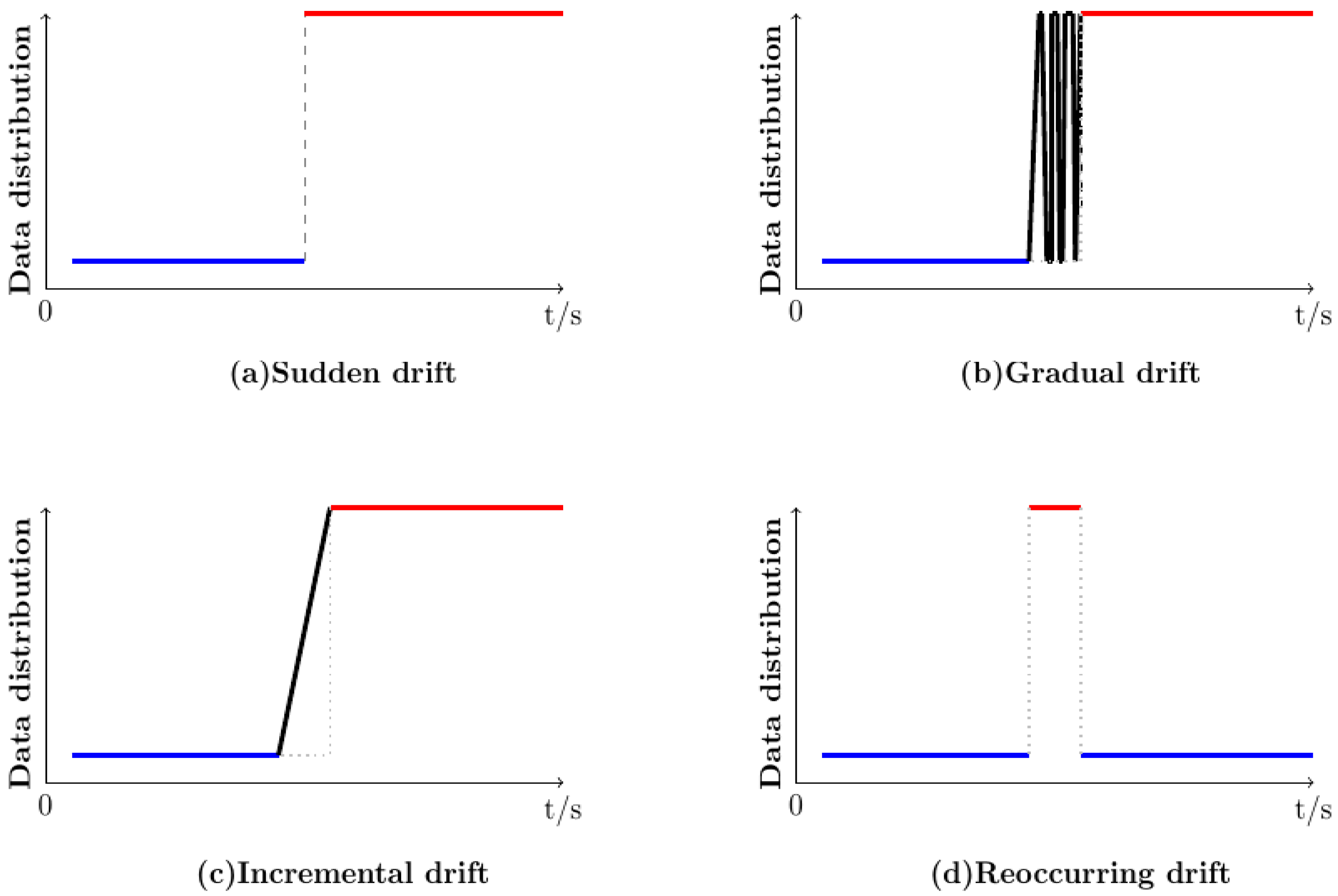
Table 1, the SEA, Sine, Mixed, and AGR datasets were generated with both abrupt and gradual drift types. According to the MOA reference manual, the HYP generator is specifically used to generate incremental data, and its method of generating drift data differs from that of the other datasets. As the classification function of the data cannot be altered, multi-drift data were not generated for the HYP dataset. All datasets contain 10,000 instances and are balanced binary-class datasets. Taking the SEA dataset as an example, when the drift position is set to 5000 and the width to 1, an abrupt SEA is generated. In this case, data before point 5000 correspond to the old concept, while data after point 5000 correspond to the new concept. When the drift position is set to 4500 and the width to 1000, a gradual SEA is generated. In this scenario, data before point 4500 correspond to the old concept, and drift begins at point 4500, lasting for 1000 instances. After point 5500, the drift ends, and the remaining data correspond to the new concept.
The datasets used in Table 2 are the same as those in Table 1, with the distinction that each dataset contains multiple drifts points and multiple instances of abrupt or gradual drift within the same data volume. In MOA, the SEA and Sine datasets each contain four classification functions (i.e., four different concepts), so we evenly divided the ten thousand data instances among the four concepts, which included three drift points. The AGR dataset contains ten classification functions, resulting in nine drift points, and the drift width for gradual AGR is smaller than for other gradual datasets. The mixed dataset contains only two classification functions, and we utilized it to generate multiple abrupt drifts datasets. So, to maintain consistency with the data volume of the other datasets, we divided the ten thousand data instances into five parts, with four points. For datasets such as SEA that contain multiple abrupt drifts, the concepts follow a step-like progression, meaning each newly appearing concept differs from all the preceding ones, forming entirely new concepts. However, due to the mixed dataset only containing two concepts, the generated data cannot include multiple concepts. As a result, in the case of multiple abrupt drifts, the data from the mixed dataset alternate between the old and new concepts.
To validate the effectiveness of the algorithm proposed in this paper, experiments were also conducted on real-world datasets. The details of the real-world datasets are as follows:
  • Weather Dataset (ftp://ftp.ncdc.noaa.gov/pub/data/gsod(accessed on 5 March 2023)): This dataset contains 18,159 samples and 8 features and is a binary classification dataset. Each feature represents information such as wind speed, temperature, and visibility on a given day, while the class label indicates whether it rained that day.
  • Electricity Dataset (https://moa.cms.waikato.ac.nz/datasets/(accessed on 5 March 2023)): This dataset comes from the Australian New South Wales Electricity Market, with data recorded every 5 min. It consists of 45,312 samples and 8 features, where each feature represents attributes such as date and price, and the label indicates whether the electricity price increased.
  • Usenet1 and Usenet2 Datasets (http://mlkd.csd.auth.gr/concept_drift.html(accessed on 1 March 2023)): These two datasets describe twenty streams of data from newsgroups, simulating the data streams from twenty different newsgroups.
  • Email Data Dataset (link in footnote 3): This dataset is a stream containing 1500 samples and 913 features. The classification task is to determine whether the user is interested in the current email.
  • NSL-KDD Dataset (https://kdd.ics.uci.edu/databases/kddcup99/kddcup99.html (accessed on 24 February 2025)): This dataset was used in the Third International Knowledge Discovery and Data Mining Tools Competition. It consists of 41 features and 35,141 instances, with the classification task aimed at identifying the type of network attacks.
For real-world data, we selected five real-world datasets with unknown drift points, along with one dataset (NSL-KDD) where drift can be verified, to validate the effectiveness of our proposed method. It is important to note that the original NSL-KDD dataset contains 4,898,431 instances, and the official dataset repository explicitly states that the distribution of the test set differs from that of the training set. Additionally, due to storage constraints, following the processing method in [37], we conducted experiments using only 10% of the training data combined with the test data. Although real-world datasets commonly used for concept drift detection typically exhibit distributional changes, the exact drift locations are unknown, making it challenging to accurately assess the detection algorithm’s performance. Guo et al. [13] evaluated the detection delay performance of the algorithm by introducing artificial drift points. Inspired by this approach, this study adopts a similar strategy of embedding drift points to assess the accuracy of drift detection algorithms on real-world datasets. Different strategies were employed for inserting drift points into real-world data with unknown drift benchmarks. When inserting a single drift point, we divided the data into three equal parts: the first one-third is used for pretraining, and this portion of the data remains unchanged. For the remaining two-thirds of the data, the first one-third is left unprocessed to ensure consistency with the distribution of the old concept (i.e., the first one-third). For the final one-third, we use a random function to select a random column and assign its feature values to random numbers between 0 and 1. Details of the datasets can be found in Table 3.
To insert multiple drift points into real-world data, the dataset is divided into five equal parts: the first one-fifth is used for pretraining and remains unchanged, while the second one-fifth also remains unchanged. In the remaining three-fifths, a random function selects a different feature column for each portion (without repetition) and replaces its values with random numbers between 0 and 1. Details on multi-drift data can be found in Table 4.

4.2. Methods for Comparison

This paper compares the proposed drift detection method, which combines deep neural networks and autoencoders, with existing classical detection methods, all of which are available from the skmultiflow (https://scikit-multiflow.readthedocs.io/en/stable/api/api.html(accessed on 28 July 2023)) library. scikit-multiflow [38] is a Python package designed for handling stream data problems. The following is a brief introduction to these methods:
  • DDM [11]: This algorithm primarily monitors the model’s error rate to detect drift. During the detection process, it continuously updates the minimum error rate and its corresponding standard deviation. If the current error rate exceeds the sum of the minimum error rate and three times the minimum standard deviation, concept drift is detected, and the minimum error rate and standard deviation are updated accordingly.
  • EDDM [20]: An improved version of DDM that refines the drift detection criteria to enhance performance.
  • HDDM_W [21]: Utilizes McDiarmid’s bound and EWMA statistics to assess the presence of drift.
  • ADWIN [12]: This method dynamically adjusts the window size, calculates statistical differences between two sub-windows, and triggers drift detection when the difference exceeds a predefined threshold.

4.3. Evaluation Metrics

For concept drift detection, commonly used evaluation metrics are employed to assess the performance of drift detection algorithms. Specifically, we utilize the first two metrics from [34,39] to evaluate the algorithm’s effectiveness in terms of detection delay and accuracy. In the case of a single drift, the First Effective Drift Point (FEDP) metric is used to quantify the effectiveness of the drift detection algorithm. The calculation is as follows:
F E D P = i = 1 n ( D P p o s ) / n
D P represents the first detected drift point that is greater than or equal to the actual drift onset, while p o s denotes the true drift start point. This metric primarily evaluates the algorithm’s ability to promptly detect drift and measure the corresponding detection delay. If no drift point is recorded in the drift list during detection, D P is set to 10,000 or 100,000. For instance, if the dataset in use is the abrupt SEA, p o s is 5000, and the first detected drift point exceeding this threshold is 5012, then F E D P is calculated as FEDP = 5012 − 5000 = 12. This represents a single F E D P result. To obtain the final evaluation, the average F E D P value is computed over n experiments.
For multiple drifts, the Effective Drift Detection Rate ( E D D R ) metric [34,39] is used to measure the number of effective detections made by the algorithm. Initially, the Effective Drift Range ( E D R ) is defined to limit the range for effective detection. For synthetic data with gradual and incremental drifts, parameters are set at the data generation stage to determine their values. Thus, the E D R for these datasets is tied to the drift formation width, as outlined in Table 1. However, for abrupt synthetic datasets, where the drift width is 1, we extend the effective drift span by 100 to maintain consistency with other datasets. This results in an E D R of (5000, 5100). For real-world datasets, whether involving single or multiple drifts, the drift’s effective range is set to a span of 100. In cases of multiple drifts, the effective range encompasses multiple points.The Effective Detected Drift Rate ( E D D R ) is used as an evaluation metric for multiple drift points. Assume DP = {DPi, DPi+1, …, DPi+t}, where D P represents all drift points detected within the effective range:
v a l i d d e t e c t e d = 1 , if D P & D P E D R | D P | / | N | , if D P & D P E D R 0 , o t h e r s
E D D R = 1 n i = 1 n v a l i d d e t e c t e d
Let N represent the number of effective ranges. A valid detection occurs only when the detected drift points are non-empty and all detected points lie within the effective range. When both conditions are satisfied, it is counted as 1. If only one or a few of the effective ranges contain valid detected drift points, the value is recorded as | D P | / | N | , which represents the number of detected drift points within the effective range (with each range counted only once) divided by the total number of effective ranges. When no drift points in the D P are within the effective range, the value is recorded as 0. This metric evaluates whether the detection algorithm can identify all drift points when multiple drifts are present, thereby assessing the sensitivity of the detection algorithm.
To measure the significant differences between algorithms, the statistical tests proposed in [40,41]—the Friedman test and its subsequent Bonferroni-Dunn test—are employed to compare the overall performance of the algorithms. First, the Friedman test is applied to verify whether all algorithms perform similarly. Suppose there are k algorithms tested on N datasets, and the variable
T X ( 2 = 12 N k ( k + 1 ) [ i = 1 k r i 2 k ( k + 1 ) 2 4 ]
When both k and N are large, T X ( 2 follows a chi-squared distribution with k 1 degrees of freedom. To improve the rigor of the test, we employ the following statistic:
T F = ( N 1 ) T X ( 2 N ( k 1 ) T X ( 2
where T X ( 2 is calculated using Equation (7). The statistic T F follows an F-distribution with degrees of freedom ( k 1 ) and ( k 1 ) ( N 1 ) .
If the null hypothesis that “all algorithms perform equally” is rejected, we proceed with the Bonferroni–Dunn test to identify significant differences between pairs of algorithms. The Bonferroni–Dunn test determines the critical difference for the mean rank differences as follows:
C D = q α k ( k + 1 ) 6 N
where q α is determined by the significance level α and and the number of algorithms k.
The false detection rate ( F D R ) is an important metric for evaluating the drift detection method’s ability to detect and identify drifts. Following the metric proposed in [13], the calculation of F D R is given by
F D R = { s i s i C i and s i S } S
where S represents the length of all drift detection output results and C i represents the actual inserted drift points. The F D R measures the proportion of invalid detections in the drift detection output, with smaller values indicating better drift detection performance.

4.4. Experiment Results and Analysis

To maintain consistency in the data distribution between the pretraining phase and the data before the drift, synthetic data for the pretraining phase are generated using the generators shown in Table 1. For the real data, the first 1/5 of the original dataset is used as pretraining data. The experiment is implemented using Python 3.6.5, and the neural network architecture is built with PyTorch 2.4.0. Details of the hyperparameter values involved in the construction of the neural network can be found in Table 5.
To validate the effectiveness of the proposed method, its performance is evaluated using the metrics discussed in Section 4.3. The detection methods mentioned in Section 4.2 all require the base classifier to classify the data and generate the error rate. To avoid the potential bias of relying on a single classifier, which may not fully utilize the performance of the drift detection algorithm, we use two classical classifiers from skmultiflow, namely Hoeffding Tree and Naive Bayes, as baseline classifiers for comparison, providing input for the detection algorithms. The parameter settings for each detector are set to their default values. To ensure fairness, each metric is computed with n set to 100, and the average of 100 experiments is taken.
It is important to note that during the pretraining phase, we first generate non-drift data for all datasets listed in 
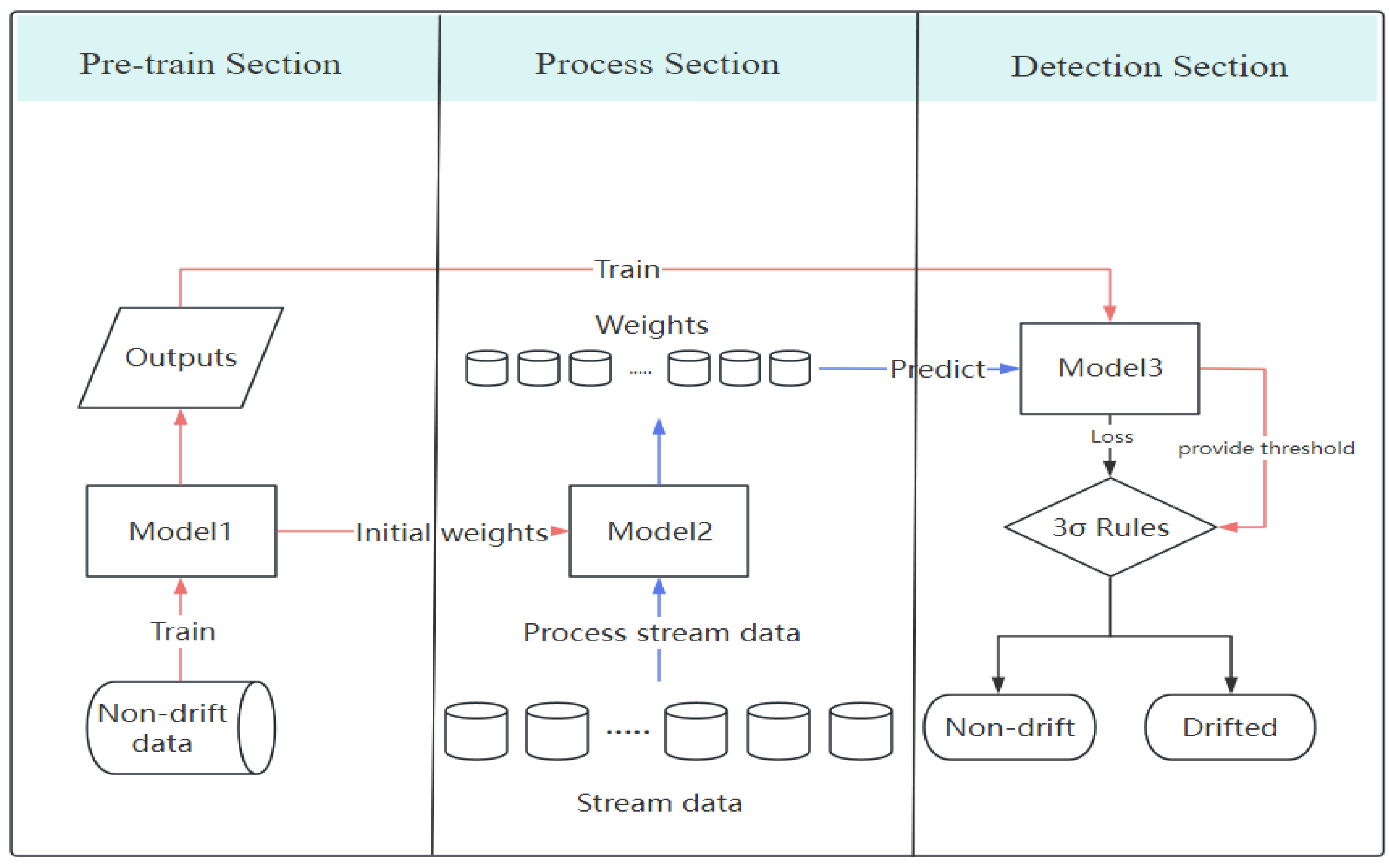
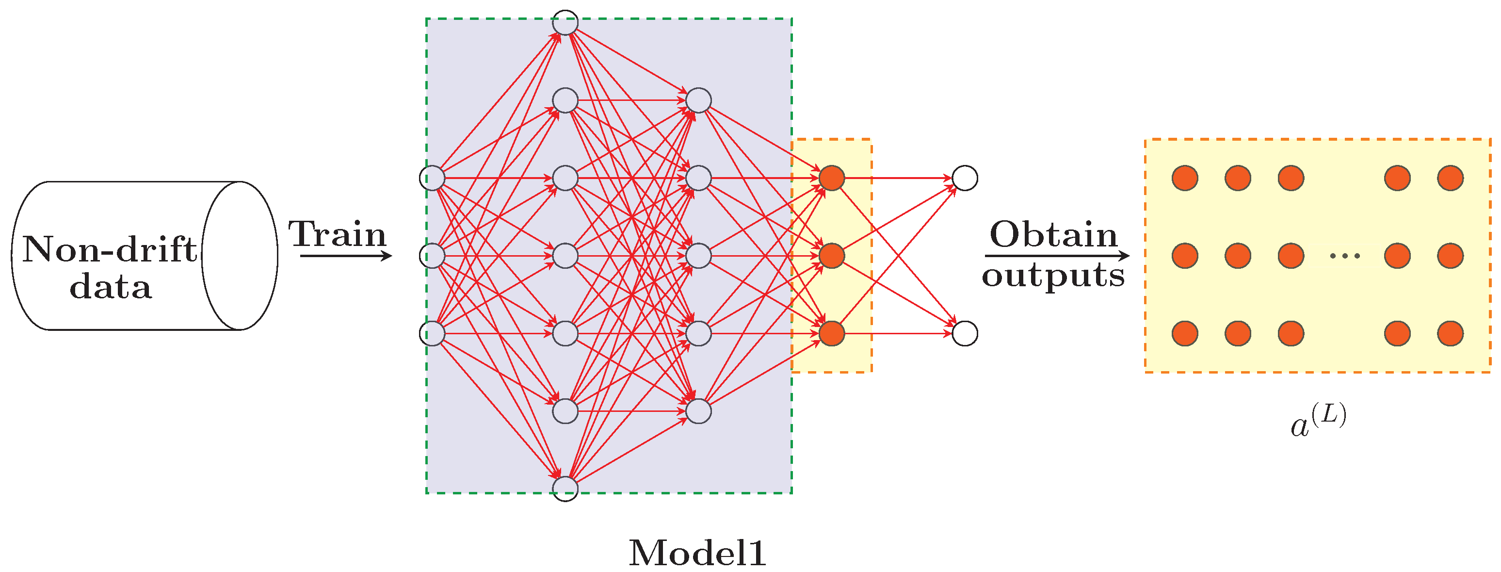
Table 1. Taking SEA_a as an example, its generation command in MOA is “WriteStreamToARFFFile -s (ConceptDriftStream -s (generators.SEAGenerator -f 3 -b -n 5000 -p 0) -d (generators.SEAGenerator -f 2 -b -n 5000 -p 0) -p 5000 -w 1) -f E:\Dataset\dataset.arff -m 10,000 -h”. The key parameter here is the value of ‘f’. The command is designed with two phases, where ‘f’ takes different values. The parameter ‘s’ represents the currently generated data stream, and when ‘f’ is set to 3 following ‘s’, the generated data are produced using generation function 3. The parameter ‘d’ denotes drift data, and the data within its parentheses is generated using function 2. Correspondingly, the non-drift SEA data are the data produced when ‘f’ is set to 3. The same approach applies to other datasets. During the pretraining phase, Model1 in 
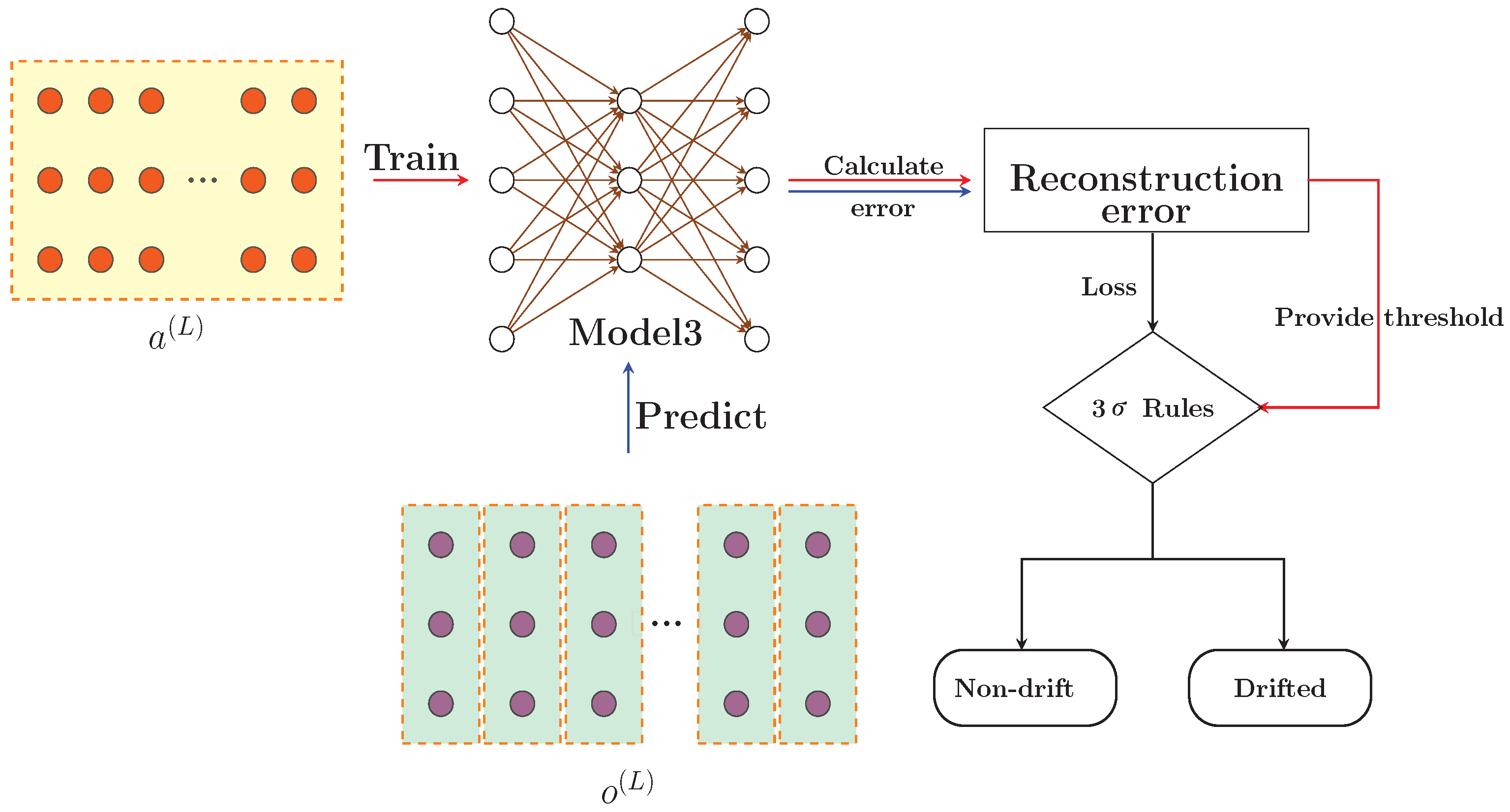
Figure 3 is trained using non-drift data generated with ‘f’ set to 3. In the streaming data processing phase, Model2 in Figure 4 processes the drift data generated by the above command.
The detection results of synthetic data with single drift using the F E D P metric are shown in Table 6. The F E D P metric represents detection delay, with smaller values being preferred. The best results in the table are highlighted in bold. From Table 6, we can observe that the performance of the detectors varies depending on the base classifier selected for different datasets. While the DNN+AE-DD method shows slightly weaker performance on certain datasets, it outperforms other methods in overall performance. The maximum value in Table 6 is 5500, indicating that the detector did not produce any output for this dataset. This suggests that drift occurred, but the detector failed to detect it. The inability of certain detection algorithms to detect drift on datasets such as AGR_g may be due to the inherent classification difficulty of the AGR dataset. Even with multiple classifiers trained on this dataset, the classification accuracy remains poor.
Assuming all algorithms perform equally, we obtain T F = 4.66 based on Equation (8). When k = 9 and N = 9 , T F follows an F-distribution with degrees of freedom (8, 64), with a critical value of 2.087. Therefore, we reject the hypothesis that all algorithms perform equally. At a confidence level of α = 0.05 , q α = 2.724 , resulting in a critical difference ( C D ) value of 3.51. The statistical results are shown in Figure 6. As observed in the figure, the proposed algorithm performs significantly better than EDDM_NB, DDM_HT, DDM_NB, and EDDM_HT in terms of delay detection.
In Figure 7, each plot corresponds to a different dataset from Table 6. The vertical axis represents the F E D P metric calculated by Equation (4), with the values on the axis represented as powers of 2 n . The horizontal axis lists the algorithms from left to right: DNN+AE-DD, DDM_NB, DDM_HT, EDDM_NB, EDDM_HT, HDDM_W_NB, HDDM_W_HT, ADWIN_NB, and ADWIN_HT. In Figure 7, two distinct colors are used to represent the delay, with orange indicating the best result for the current metric (for values exceeding 10,000, 10,000 is used for representation). The observation results reveal that the DNN+AE-DD algorithm performs particularly well on certain datasets, such as reducing the detection delay to a very small range on datasets like HYP. Other algorithms also demonstrate optimal performance on various datasets. Therefore, we can conclude that the DNN+AE-DD is effective in detecting concept drift in the case of a single drift occurrence.
In Figure 7, the performance of the DNN+AE-DD in detecting abrupt concept drift is generally inferior to that of other algorithms across most datasets. The possible reason for this could be the short duration of abrupt drift events, making them harder to detect, or the overlap between the distributions of old and new concepts, which complicates detection in the short term. This hypothesis is further supported by the observation of the DNN+AE-DD’s performance on other datasets with gradual and incremental drifts. In gradual and incremental drift scenarios, there is a transitional period during which the data distribution changes over time. Specifically, in gradual drift, data points from the new distribution gradually increase, while data from the old distribution decrease. The classification boundaries between the old and new distributions may overlap during this transition, which can cause detection delays. As a result, the detection performance of the algorithm may vary across different datasets. For incremental drift data, the data in the transitional period do not belong strictly to either the new or old distribution, which allows the DNN+AE-DD to detect the drift with relatively shorter delay.
The data in Table 7 show the performance of various algorithms on the E D D R metric for synthetic multi-drift data. An ideal result for this metric is a value close to 1.0, with the best results highlighted in bold. This metric illustrates that each drift detection algorithm has its optimal performance at specific moments, but overall, the method proposed in this paper performs well. A value of 0.0 in Table 7 may indicate that the current detector did not identify values within the valid detection range for a particular dataset. In such cases, the detector might have produced a result, but the detection outcome was suboptimal, or the detector might have failed to detect the occurrence of drift.
Based on Equation (8), we obtain T F = 3.80 . When k = 9 and N = 7 , T F follows an F-distribution with degrees of freedom (8, 48), with a critical value of 2.138, leading us to reject the hypothesis that “all algorithms perform equally”. At a confidence level of α = 0.05 , q α = 2.724 , yielding a critical difference ( C D ) value of 3.99. The statistical results are shown in Figure 8. As seen in the figure, the proposed algorithm significantly outperforms DDM_NB and DDM_HT in terms of effective detection metrics.
In Figure 9, the different colored bars represent different effective detection ranges. SEA and Sine each have three effective detection ranges, corresponding to three colored bars, while mixed has four effective detection ranges and AGR has nine effective detection ranges. The results in Table 7 represent the average values for each effective detection range (with an average value of 1.0 only when all bars have a value of 1.0). Figure 9 presents detailed results for each effective detection range. From the figure, when facing multiple abrupt/gradual drift datasets, we can observe that although the DNN+AE-DD does not guarantee the best performance across all datasets, it performs well on most abrupt/gradual drift datasets. For example, in AGR_a and SEA_g, despite not achieving the best results on datasets like Sine_a, it ensures that a valid output is detected within each effective detection range. In cases where optimal performance is not achieved, this may be due to one or more detection instances failing to produce an output or providing an unsatisfactory result.
Table 8 and Table 9 present the F E D P and E D D R outputs for the detection algorithm on real-world datasets with single and multiple drifts, respectively. Due to the varying sizes of the real datasets, we set the drift point outputs to 100,000 for algorithms that fail to detect drift, leading to larger values in Table 8. The best outcomes are highlighted in bold. From these tables, it can be observed that the DNN+AE-DD algorithm demonstrates strong overall performance on both single-drift and multiple-drift real-world datasets. While our algorithm does not always achieve optimal performance on certain datasets, its results are only slightly below the best cases. These findings further validate the effectiveness of the DNN+AE-DD algorithm in detecting concept drift in streaming data.
In Figure 10, the computed value of T F is 3.28. When k = 9 and N = 6 , T F follows an F-distribution with degrees of freedom (8, 40), with a critical value of 2.18. This result leads to the rejection of the null hypothesis that “all algorithms perform equally”. At a confidence level of α = 0.05 , the critical value q α is 2.724, yielding a critical difference ( C D ) value of 4.31. As illustrated in the figure, the proposed algorithm demonstrates significantly better performance in terms of delay detection compared to the DDM_NB, DDM_HT, ADWIN_NB, and ADWIN_HT.
In Figure 11, the computed value of T F is 6.62. When k = 9 and N = 5 , T F follows an F-distribution with degrees of freedom (8,32), with a critical value of 2.244. This result also leads to the rejection of the null hypothesis that “all algorithms perform equally”. At a confidence level of α = 0.05 , the critical value q α is 2.724, yielding a C D value of 4.72. As shown in the figure, the proposed algorithm significantly outperforms the DDM_HT, ADWIN_NB, and ADWIN_HT in terms of the effective detection range.
In Figure 12, the orange color represents the algorithm with the best detection delay performance, while the other algorithms are depicted in blue. When detecting a single drift, the DNN+AE-DD is able to significantly reduce detection delay across most real-world datasets. However, on the NSL-KDD dataset, the delay for nearly all classifiers is notably longer compared to other datasets. By analyzing Figure 12 and Figure 13, we observe that when detecting multiple drifts, the DNN+AE-DD algorithm performs slightly worse than detectors such as EDDM on the Electricity dataset. However, it demonstrates superior overall performance across different datasets. In the case of artificial drift points implanted in real-world datasets, the DNN+AE-DD demonstrates a clear advantage in detecting abrupt drifts. However, due to the inherent complexity of real-world data, the detection delay varies. Furthermore, we observe that the performance of the detector varies depending on the classifier chosen, highlighting the significant impact of base classifier selection on drift detection performance. For most classifiers, other detectors perform poorly, which may be attributed to the complex and dynamic nature of real-world data. Since the detector’s input relies on the predictions of the base classifier, fluctuations introduced by drift points may cause the classifier to mislabel data as noise, potentially resulting in the absence of detection outputs.
Based on the experimental results, the proposed DNN+AE-DD method effectively and promptly detects concept drift with minimal delay while demonstrating the capability to identify multiple types of drift.
Furthermore, for the synthetic datasets in Table 10, we conducted a comparison of the false detection rates ( F D R ) across different algorithms, with the results presented in Table 10. For cases where the algorithm did not produce detection output in all 100 experiments, we assigned the value “NaN”. The values in the table are expressed as percentages.
From Table 10, it can be observed that the DNN+AE-DD effectively detected drift across all datasets in one hundred experiments (i.e., no “NaN” results), whereas other algorithms exhibited “NaN” on one or more datasets. This demonstrates the robustness of the proposed method in detecting drifts across various datasets and drift types. While different algorithms perform optimally on different datasets, the DNN+AE-DD maintains a balanced performance. Although the DNN+AE-DD does not achieve the lowest false detection rate when compared to all algorithms, its false detection rate is comparable or even better than the comparisons. For instance, on the AGR_a, AGR_g and HYP_i datasets, most methods fail to detect drift effectively, whereas the DNN+AE-DD successfully identifies drift in all 100 experiments with a relatively low false detection rate. In summary, although the performance of the DNN+AE-DD varies across datasets compared to other algorithms, it consistently detects drift with shorter delays and strong robustness.

5. Conclusions and Future Work

To address concept drift in online scenarios such as fraud detection, healthcare, and industrial equipment maintenance, this paper proposes a concept drift detection method based on deep neural networks and autoencoders (DNN+AE-DD). The method employs a deep neural network as the base classifier, initially trained on static data. After training, the hidden layer outputs are collected to generate training data for the autoencoder. During testing, the autoencoder processes hidden layer outputs from streaming data. Once trained (initialized), the 3 σ principle is applied to determine whether drift has occurred. The proposed method is compared with several classical drift detection techniques, demonstrating its timeliness and effectiveness in handling various types of drifts, including single and multiple drifts. The results indicate that the method enhances drift detection sensitivity, ensuring robust performance across different datasets.
Despite the proposed algorithm demonstrating significant advantages in detection delay and other aspects, it still has certain limitations in the following areas:
  • The computational complexity of the DNN+AE-DD algorithm is relatively high, primarily due to the iterations and backpropagation during the training process. In contrast, other algorithms are not constrained by this bottleneck. Future work will focus on optimizing the efficiency of the training process to mitigate this challenge.
  • This study focuses solely on experiments with traditional feedforward neural networks and does not include models widely used in the current deep learning field, such as deep recurrent neural networks. Furthermore, due to the relatively simple model structure, techniques such as model compression are not addressed in this study. Compared to feedforward neural networks, recurrent neural networks can more effectively capture long-term and short-term dependencies in data and have the ability to retain historical information. Therefore, they may have significant potential advantages in addressing recurring concept drift. In the future, we will conduct experiments using large models on ultra-large-scale datasets and perform in-depth research by integrating different types of networks and transfer learning. Additionally, we will design detailed optimization techniques such as knowledge distillation and model compression, aiming to discover and develop more effective detection algorithms.
  • This algorithm is specifically designed for detecting concept drift. In related work, we discussed that current approaches to addressing concept drift problems primarily fall into two categories: drift detection and model adaptation. Integrating drift detection with model adaptation can accelerate a model’s adaptation to new data distributions while enhancing its generalization ability. In future work, we plan to leverage the detection outputs of this algorithm for model adaptation, aiming to improve the model’s robustness and adaptability in handling concept drift.
  • This approach assumes an idealized scenario where the model operates without missing data, noisy data, adversarial data, or feature evolution. However, these challenges are more prevalent and hold greater practical significance in real-world streaming data applications. Addressing missing values, enhancing robustness to noisy data, improving resistance to adversarial data, and designing models to accommodate feature evolution are crucial research directions. In future work, we aim to develop more comprehensive solutions to tackle these complex data scenarios.

Author Contributions

Conceptualization, L.H.; methodology, L.H. and Y.L.; software, Y.L.; validation, L.H., Y.L. and Y.F.; formal analysis, Y.F.; investigation, Y.F.; resources, L.H.; data curation, Y.L.; writing—original draft preparation, Y.L.; writing—review and editing, Y.L.; visualization, Y.L.; supervision, L.H.; project administration, L.H.; funding acquisition, L.H. All authors have read and agreed to the published version of the manuscript.

Funding

This research was funded by the Central Government’s Fund for Guiding Local Technological Development Project of Hebei Province (No. 246Z0703G), the Science Research Project of Hebei Education Department (QN2023184), the Base Research Project for Colleges and Universities in Hebei Province in Shijiazhuang City (241791057A), and the Scientific Research and Development Plan Project of Hebei University of Economics and Business (2022ZD10).

Institutional Review Board Statement

Not applicable.

Informed Consent Statement

Not applicable.

Data Availability Statement

The raw data supporting the conclusions of this article will be made available by the authors on request.

Conflicts of Interest

The authors declare no conflicts of interest.

Appendix A

To demonstrate that the weights in Figure 4 have been updated through error backpropagation, the following presents scatter plots of the mean weights before and after data drift, using the Sine_a and Mixed_a datasets as representatives.
By observing the below figure, it is evident that there is a noticeable change in the mean values of the hidden layer weights before and after the drift.
For the experiments, we conducted validation with different drift thresholds, and the results are presented in Table A1.
The results in Table A1 show that when a broader drift threshold is used, the false detection rate of the DNN+AE-DD algorithm increases accordingly.
Figure A1. Weights changes of Sine_a.
Applsci 15 03056 g0a1
Figure A2. Weights changes of Mixed_a.
Applsci 15 03056 g0a2
Table A1. FDR for different drift thresholds.
Datasets μ 3 σ μ 2 σ μ σ
Sine_a0.390.480.52
SEA_a0.350.350.45
AGR_a0.240.430.50
Sine_g0.380.430.45
SEA_g0.300.380.40
Mixed_g0.300.300.46
AGR_g0.390.390.46

References

  1. Olan, F.; Jayawickrama, U.; Arakpogun, E.O.; Suklan, J.; Liu, S. Fake news on social media: The impact on society. Inf. Syst. Front. 2024, 26, 443–458. [Google Scholar] [CrossRef] [PubMed]
  2. Modgil, S.; Singh, R.K.; Gupta, S.; Dennehy, D. A confirmation bias view on social media induced polarisation during Covid-19. Inf. Syst. Front. 2024, 26, 417–441. [Google Scholar] [CrossRef]
  3. Chatterjee, P.; Das, D.; Rawat, D.B. Digital twin for credit card fraud detection: Opportunities, challenges, and fraud detection advancements. Future Gener. Comput. Syst. 2024, 158, 410–426. [Google Scholar] [CrossRef]
  4. Charizanos, G.; Demirhan, H.; İçen, D. An online fuzzy fraud detection framework for credit card transactions. Expert Syst. Appl. 2024, 252, 124127. [Google Scholar] [CrossRef]
  5. Mienye, I.D.; Jere, N. Deep learning for credit card fraud detection: A review of algorithms, challenges, and solutions. IEEE Access 2024, 12, 96893–96910. [Google Scholar] [CrossRef]
  6. Tang, Y.; Liang, Y. Credit card fraud detection based on federated graph learning. Expert Syst. Appl. 2024, 256, 124979. [Google Scholar] [CrossRef]
  7. Schlimmer, J.C.; Granger, R.H. Incremental learning from noisy data. Mach. Learn. 1986, 1, 317–354. [Google Scholar] [CrossRef]
  8. Losing, V.; Hammer, B.; Wersing, H. KNN classifier with self adjusting memory for heterogeneous concept drift. In Proceedings of the 2016 IEEE 16th International Conference on Data Mining, Barcelona, Spain, 12–15 December 2016; pp. 291–300. [Google Scholar]
  9. Meng, F.; Han, M.; Li, C.; Zhang, R.; He, F. Survey of Concept Drift Detection and Adaptation Methods. J. Comput. Eng. Appl. 2024, 60, 75–88. [Google Scholar]
  10. Sun, Z.; Tang, J.; Qiao, J. Semi-supervised concept drift detection method by combining sample output space and feature space with its application. Acta Autom. Sin. 2022, 48, 1259–1272. [Google Scholar]
  11. Gama, J.; Medas, P.; Castillo, G.; Rodrigues, P. Learning with drift detection. In Proceedings of the Advances in Artificial Intelligence–SBIA 2004: 17th Brazilian Symposium on Artificial Intelligence, Sāo Luis, Brazil, 29 September–1 October 2004; pp. 286–295. [Google Scholar]
  12. Bifet, A.; Gavalda, R. Learning from time-changing data with adaptive windowing. In Proceedings of the 2007 SIAM international conference on data mining, Minneapolis, MN, USA, 26–28 April 2007; pp. 443–448. [Google Scholar]
  13. Guo, H.; Zhang, A.; Wang, W. Concept drift detection method based on online performance test. J. Softw. 2020, 31, 932–947. [Google Scholar]
  14. Jain, M.; Kaur, G.; Saxena, V. A K-Means clustering and SVM based hybrid concept drift detection technique for network anomaly detection. Expert Syst. Appl. 2022, 193, 116510. [Google Scholar] [CrossRef]
  15. Gama, J.; Žliobaitė, I.; Bifet, A.; Pechenizkiy, M.; Bouchachia, A. A survey on concept drift adaptation. ACM Comput. Surv. (CSUR) 2014, 46, 1–37. [Google Scholar] [CrossRef]
  16. Yu, H.; Zhang, Q.; Liu, T.; Lu, J.; Wen, Y.; Zhang, G. Meta-ADD: A meta-learning based pre-trained model for concept drift active detection. Inf. Sci. 2022, 608, 996–1009. [Google Scholar] [CrossRef]
  17. Mehmood, T.; Latif, S.; Jamail, N.S.M.; Malik, A.; Latif, R. LSTMDD: An optimized LSTM-based drift detector for concept drift in dynamic cloud computing. PeerJ Comput. Sci. 2024, 10, e1827. [Google Scholar] [CrossRef] [PubMed]
  18. Ma, Q.; Guo, H.; Wang, W. Weakly supervised concept drift detection method for online deep neural networks. J. Chin. Comput. Syst. 2024, 45, 2094–2101. [Google Scholar]
  19. Lu, J.; Liu, A.; Dong, F.; Gu, F.; Gama, J.; Zhang, G. Learning under concept drift: A review. IEEE Trans. Knowl. Data Eng. 2018, 31, 2346–2363. [Google Scholar] [CrossRef]
  20. Baena-Garcıa, M.; del Campo-Ávila, J.; Fidalgo-Merino, R.; Bifet, A.; Gavald, R.; Morales-Bueno, R. Early drift detection method. In Proceedings of the Fourth International Workshop on Knowledge Discovery from Data Streams, Philadelphia, PA, USA, 20 August 2006; pp. 77–86. [Google Scholar]
  21. Frias-Blanco, I.; del Campo-Ávila, J.; Ramos-Jimenez, G.; Morales-Bueno, R.; Ortiz-Díaz, A.; Caballero-Mota, Y. Online and non-parametric drift detection methods based on Hoeffding’s bounds. IEEE Trans. Knowl. Data Eng. 2014, 27, 810–823. [Google Scholar] [CrossRef]
  22. Raab, C.; Heusinger, M.; Schleif, F.M. Reactive soft prototype computing for concept drift streams. Neurocomputing 2020, 416, 340–351. [Google Scholar] [CrossRef]
  23. Klikowski, J. Concept drift detector based on centroid distance analysis. In Proceedings of the 2022 International Joint Conference on Neural Networks, Padua, Italy, 18–23 July 2022; pp. 1–8. [Google Scholar]
  24. de Lima Cabral, D.R.; de Barros, R.S.M. Concept drift detection based on Fisher’s Exact test. Inf. Sci. 2018, 442, 220–234. [Google Scholar] [CrossRef]
  25. Han, M.; Meng, F.; Li, C.; Zhang, R.; He, F.; Ding, J. Kolmogorov inequality based drift detection methods for data stream. J. Comput. Eng. Appl. 2024, 1–16. [Google Scholar]
  26. Qiu, X. Neural Networks and Deep Learning, 1st ed.; China Machine Press: Beijing, China, 2020; pp. 90–91. (In Chinese) [Google Scholar]
  27. Priya, S.; Uthra, R.A. Deep learning framework for handling concept drift and class imbalanced complex decision-making on streaming data. Complex Intell. Syst. 2023, 9, 3499–3515. [Google Scholar] [CrossRef]
  28. Cai, S.; Zhao, Y.; Hu, Y.; Junzhe, Y.; Wu, H.; Wu, J.; Zhang, G.; Zhao, C.; Sosu, R.N.A. CD-BTMSE: A Concept Drift detection model based on Bidirectional Temporal Convolutional Network and Multi-Stacking Ensemble learning. Knowl. Based Syst. 2024, 294, 111681. [Google Scholar] [CrossRef]
  29. Baier, L.; Schlör, T.; Schöffer, J.; Kühl, N. Detecting concept drift with neural network model uncertainty. arXiv 2021, arXiv:2107.01873. [Google Scholar]
  30. Qiu, Y.; Chang, X.; Qiu, Q.; Peng, C.; Su, S. Stream data anomaly detection method based on long short-term memory network and sliding window. J. Comput. Appl. 2020, 40, 1335. [Google Scholar]
  31. Hatamikhah, N.; Barari, M.; Kangavari, M.R.; Keyvanrad, M.A. Concept drift detection via improved deep belief network. In Proceedings of the Electrical Engineering (ICEE), Iranian Conference, Mashhad, Iran, 8–10 May 2018; pp. 1703–1707. [Google Scholar]
  32. Lin, L.; Xiao, L.; Wei, D.; Chen, W.; Di, Y.; Xu, Y.; Wang, J. Process concept drift detection based on graph convolutional network. Comput. Integr. Manuf. Syst. 2024, 30, 2735. [Google Scholar]
  33. Lin, L.; Jin, Y.; Wen, L.; Chen, W.; Di, Y.; Xu, Y.; Wang, J. Process Drift Detection in Event Logs with Graph Convolutional Networks. In Proceedings of the International Conference on Database Systems for Advanced Applications, Tianjin, China, 17–20 April 2023; pp. 380–396. [Google Scholar]
  34. Wang, P.; Jin, N.; Davies, D.; Woo, W.L. Model-centric transfer learning framework for concept drift detection. Knowl. Based Syst. 2023, 275, 110705. [Google Scholar] [CrossRef]
  35. Guo, H.; Zhang, S.; Wang, W. Selective ensemble-based online adaptive deep neural networks for streaming data with concept drift. Neural Netw. 2021, 142, 437–456. [Google Scholar] [CrossRef]
  36. Bifet, A.; Holmes, G.; Pfahringer, B.; Kranen, P.; Kremer, H.; Jansen, T.; Seidl, T. Moa: Massive online analysis, a framework for stream classification and clustering. In Proceedings of the First Workshop on Applications of Pattern Analysis, Windsor, UK, 1–3 September 2010; pp. 44–50. [Google Scholar]
  37. Yang, L.; Shami, A. A lightweight concept drift detection and adaptation framework for IoT data streams. IEEE Internet Things Mag. 2021, 4, 96–101. [Google Scholar] [CrossRef]
  38. Montiel, J.; Read, J.; Bifet, A.; Abdessalem, T. Scikit-multiflow: A multi-output streaming framework. J. Mach. Learn. Res. 2018, 19, 1–5. [Google Scholar]
  39. Wang, P.; Jin, N.; Woo, W.L.; Woodward, J.R.; Davies, D. Noise tolerant drift detection method for data stream mining. Inf. Sci. 2022, 609, 1318–1333. [Google Scholar] [CrossRef]
  40. Guo, H.; Zhang, Y.; Wang, W. Two-Stage adaptive ensemble learning method for different types of concept drift. J. Comput. Res. Dev. 2024, 61, 1799–1811. [Google Scholar]
  41. Guo, H.; Sun, N.; Wang, J.; Wang, W. Concept drift convergence method based on adaptive deep ensemble networks. J. Comput. Res. Dev. 2024, 61, 172–183. [Google Scholar]
Figure 1. Different types of concept drift.
Applsci 15 03056 g001
Figure 2. The overall workflow.
Applsci 15 03056 g002
Figure 3. Pretrain process.
Applsci 15 03056 g003
Figure 4. Processing stream data.
Applsci 15 03056 g004
Figure 5. Concept drift detection.
Applsci 15 03056 g005
Figure 6. Average rank of synthetic data with single drift based on the Bonferroni–Dunn test.
Applsci 15 03056 g006
Figure 7. Different algorithms’ comparsion on FEDP metrics of synthetic data with single drift.
Applsci 15 03056 g007
Figure 8. Average rank of synthetic data with multiple drifts based on the Bonferroni–Dunn test.
Applsci 15 03056 g008
Figure 9. Different algorithms’ comparsion on EDDR metrics of synthetic data with multiple drifts.
Applsci 15 03056 g009
Figure 10. Average rank of real-world data with single drift based on the Bonferroni–Dunn test.
Applsci 15 03056 g010
Figure 11. Average rank of real-world data with multiple drifts based on the Bonferroni–Dunn test.
Applsci 15 03056 g011
Figure 12. Different algorithms’ comparsion of FEDP metrics about real-world data with single drift.
Applsci 15 03056 g012
Figure 13. Different algorithms’ comparsion of EDDR metrics about real-world data with multiple drifts.
Applsci 15 03056 g013
Table 1. Synthetic Data with single drift.
DatasetsNumber of FeaturesNumber of SammplesDrift PositionDrift Width
SEA_a 1310,00050001
SEA_g 2310,00045001000
Sine_a210,00050001
Sine_g210,00045001000
Mixed_a410,00050001
Mixed_g410,00045001000
AGR_a610,00050001
AGR_g610,00045001000
HYP_i 31010,00045001000
1 The word ‘a’ mentioned means the type of drift is abrupt. 2 The word ‘g’ mentioned means the type of drift is gradual. 3 The word ‘i’ mentioned means the type of drift is incremental.
Table 2. Synthetic data with multiple drifts.
DatasetsNumber of FeaturesNumber of SamplesDrift PositionsDrift Width
SEA_a310,0002500, 5000, 75001
SEA_g310,0002000, 4500, 70001000
Sine_a210,0002500, 5000, 75001
Sine_g210,0002000, 4500, 70001000
Mixed_A 4410,0002000, 4000, 6000, 80001
AGR_a610,0001000, 2000, 3000, 4000, 5000, 6000, 7000, 8000, 90001
AGR_g610,000900, 1900, 2900, 3900, 4900, 5900, 6900, 7900, 8900200
4 The word ‘A’ mentioned means the type of drift is multiple abrupt.
Table 3. Real-world data with single drift.
DatasetsNumber of FeaturesNumber of SamplesImbalance RatioDrift TypeDrift Position
Weather818,15968.62Abrupt6054
Electricity845,31257.55Abrupt15,105
Usenet199150053.33Abrupt501
Usenet299150066.67Abrupt501
Email data913150053.33Abrupt501
NSL-KDD4135,14153.14Abrupt12,597
Table 4. Real-world data with multiple drifts.
DatasetsNumber of FeaturesNumber of SamplesDrift Position
Weather818,1593631, 7262, 10,893
Electricity845,3129062, 18,124, 27,186
Usenet1991500300, 600, 900
Usenet2991500300, 600, 900
Email data9131500300, 600, 900
Table 5. DNN+AE-DD parameter settings.
ParameterValue
L3
M F , M S , M L 256, 128, 64
L A 8
A p 10
η 1 , η 2 , η A 1 × 10 2 , 1 × 10 4 , 1 × 10 4
s 1 , s 2 20, 10
γ 1 , γ 2 0.9, 1.0
o p t i m 1 , o p t i m 2 SGD, Adam
L P , L A BCEWithLogitsLoss/MSELoss
Table 6. FEDP on synthetic data with single drift.
DatasetsDNN+AE-DDDDMEDDMHDDM_WADWIN
NBHTNBHTNBHTNBHT
AGR_a2952.11 (4)4925.53 (6)5000.00 (8)5000.00 (8)5000.00 (8)473.00 (1)783.00 (2)4192.77 (5)2504.60 (3)
SEA_a6.12 (1)704.18 (3)4908.36 (7)4904.26 (6)124.66 (2)5000.00 (8.5)5000.00 (8.5)776.28 (4)3306.47 (5)
Sine_a11.79 (3)291.79 (7)194.57 (6)1211.62 (9)977.33 (8)8.00 (2)7.00 (1)127.64 (5)79.00 (4)
Mixed_a15.98 (3)225.16 (7)104.31 (5)1046.53 (9)408.43 (8)5.00 (1)6.00 (2)79.00 (4)110.68 (6)
AGR_g142.35 (1)1932.60 (4)5500.00 (8)5500.00 (8)5500.00 (8)495.00 (2)1287.00 (3)4093.68 (6)2305.40 (5)
SEA_g8.96 (1)1608.05 (4)5500.00 (8)1363.93 (3)322.45 (2)5500.00 (8)5500.00 (8)2681.41 (6)1668.32 (5)
Sine_g19.39 (1)1083.31 (7)712.03 (6)1872.98 (9)1113.21 (8)256.00 (2)313.00 (3)467.00 (4)467.64 (5)
Mixed_g10.71 (1)925.04 (8)518.89 (6)1660.59 (9)758.70 (7)256.00 (2)263.00 (3)323.32 (5)307 (4)
HYP_i1.00 (1)5500.00 (7.5)5500.00 (7.5)460.00 (3)389.82 (2)5500.00 (7.5)5500.00 (7.5)4892.18 (4)4937.60 (5)
Average rank1.785.946.837.115.893.784.224.784.67
The word with bold represent the best result.The same applies to the following tables.
Table 7. EDDR on synthetic data with multiple drifts.
DatasetsDNN+AE-DDDDMEDDMHDDM_WADWIN
NBHTNBHTNBHTNBHT
AGR_a0.98 (1)0.00 (6.5)0.00 (6.5)0.00 (6.5)0.04 (3)0.00 (6.5)0.00 (6.5)0.00 (6.5)0.09 (2)
SEA_a0.87 (1)0.00 (6)0.00 (6)0.00 (6)0.00 (6)0.00 (6)0.00 (6)0.01 (2)0.00 (6)
Sine_a0.86 (3)0.01 (6.5)0.00 (8.5)0.01 (6.5)0.00 (8.5)0.67 (4.5)1.00 (1.5)1.00 (1.5)0.67 (4.5)
AGR_g0.96 (1)0.0 (8)0.0 (8)0.11 (5)0.17 (4)0.22 (3)0.44 (2)0.06 (6)0.0 (8)
SEA_g0.83 (1)0.01 (5.5)0.00 (8)0.67 (2)0.01 (5.5)0.00 (8)0.00 (8)0.04 (4)0.06 (3)
Sine_g0.86 (3)0.5 (7)0.67 (5)0.00 (9)0.33 (8)0.67 (5)0.67 (5)1.00 (1.5)1.00 (1.5)
Mixed_A0.98 (4)0.00 (8.5)0.25 (7)0.00 (8.5)0.38 (6)0.50 (5)1.00 (2)1.00 (2)1.00 (2)
Average rank2.06.867.06.215.865.434.433.363.86
Table 8. FEDP comparison of real-world data with single drift.
DatasetsDNN+AE-DDDDMEDDMHDDM_WADWIN
NBHTNBHTNBHTNBHT
Weather1.0 (1)93,946.00 (8.5)93,946.00 (8.5)64.00 (4)93017.20 (7)23.00 (2)28.00 (3)685.84 (6)579.60 (5)
Electricity2.02 (1)4.00 (2)69.00 (6)9.00 (3)56.00 (5)105.00 (7)53.00 (4)126.00 (8)158.00 (9)
Usenet11.08 (1)49,923.99 (8)49,907.98 (7)344.51 (5)343.05 (4)247.00 (2.5)247.00 (2.5)68,722.21 (9)7940.50 (6)
Usenet24.3 (1)415.99 (6)416.53 (7)344.79 (3)332.96 (2)400.00 (4.5)400.00 (4.5)99,499.00 (8.5)99,499.00 (8.5)
Email data8.35 (1)99,499.00 (8)49,913.00 (5)293.72 (3)286.95 (2)99,499.00 (8)99,499.00 (8)27,106.43 (4)75,675.40 (6)
NSL-KDD34.37 (1)2725.05 (5)451.76 (2)86,539.01 (7)86,538.48 (6)87,403.0 (8.5)87,403.0 (8.5)995.14 (4)453.38 (3)
Average rank1.06.255.924.174.335.425.086.586.25
Table 9. EDDR comparison of real-world data with multiple drifts.
DatasetsDNN+AE-DDDDMEDDMHDDM_WADWIN
NBHTNBHTNBHTNBHT
Weather1.00 (1)0.00 (7)0.00 (7)0.33 (2.5)0.00 (7)0.00 (7)0.33 (2.5)0.17 (4)0.00 (7)
Electricity0.69 (3)0.33 (6)0.00 (9)1.0 (1.5)1.0 (1.5)0.67 (4.5)0.67 (4.5)0.06 (8)0.08 (7)
Usenet10.90 (1)0.00 (8.5)0.00 (8.5)0.49 (2)0.17 (5)0.33 (3.5)0.33 (3.5)0.08 (7)0.16 (6)
Usenet21.0 (1)0.17 (6.5)0.17 (6.5)0.33 (4.5)0.33 (4.5)0.67 (2.5)0.67 (2.5)0.06 (9)0.08 (8)
Email data0.96 (1)0.66 (4.5)0.66 (4.5)0.33 (6.5)0.33 (6.5)0.67 (2.5)0.67 (2.5)0.17 (8)0.00 (9)
Average rank1.46.57.13.44.94.03.17.27.4
Table 10. FDRs of synthetic data with single drift.
DatasetsDNN+AE-DDDDMEDDMHDDM_WADWIN
NBHTNBHTNBHTNBHT
Sine_a38.540.00.00.50.50.049.549.50.0
SEA_a35.100.0NaNNaN66.71NaNNaN49.5NaN
Mixed_a47.590.00.00.430.770.00.049.50.0
AGR_a23.66NaNNaNNaNNaN44.4471.38NaN49.5
Sine_g37.360.00.00.560.470.00.033.00.0
SEA_g29.750.0NaN13.2648.89NaNNaN3.5NaN
Mixed_g30.360.00.50.160.40.00.024.750.0
AGR_g38.53NaNNaNNaN1.037.579.95NaN49.5
HYP_i41.59NaNNaN41.6553.86NaNNaNNaNNaN
Disclaimer/Publisher’s Note: The statements, opinions and data contained in all publications are solely those of the individual author(s) and contributor(s) and not of MDPI and/or the editor(s). MDPI and/or the editor(s) disclaim responsibility for any injury to people or property resulting from any ideas, methods, instructions or products referred to in the content.

