Comparative Analysis of In-Plane and Out-of-Plane Bending Benchmarks Using Two Finite Element Packages

Abstract

An essential aspect of design from the perspective of structural strength is the reliability of the results obtained during the computations for the analyzed model. Among various skills in numerical analysis, an engineer should be able to independently verify the quality of the available software using benchmarks already at the level of statics. An effective method of such verification is comparing the test results obtained from two different packages. The paper discusses three structure-oriented benchmarks for in-plane and out-of-plane bending of a flat membrane and a slab, respectively. The computations are carried out using the Robot and Midas finite element tools. These simulation tests are selected to present issues related to the modeling of bending, which is crucial for reliable design: the convergence of the solution for a cantilever, the possibility of a reduction in slab moments above columns, and the interaction effects between the beam and the plate, depending on their position and connection in the model. It is shown that, in finite element calculations, attention must be paid to avoiding errors due to improper data input and software option settings, leading to incorrect simulation results, which may negatively impact the design process. A proper understanding of software tools, for example, through benchmark verification, ensures their conscious use in developing more complex structural models.

1. Introduction

The modern designer of civil engineering structures works with a wide range of CAD (computer-aided design) software and applications that allow one to carry out static or more advanced analysis, structural element dimensioning, and the preparation of documentation. The proficient use of computer programs in engineering necessitates not only the knowledge of the basics of mechanics and numerical methods but also a deep comprehension of the modeling capabilities offered by the tools employed. These tools constitute a group of interrelated conceptual artifacts, such as implemented principles, concepts, or algorithms, which help, through their functionality, to manage the complexity of both modeling and models; see [1]. This approach establishes a mutual connection between the simplicity of the available software tools and the complexity of the constructed models. The integration of theoretical knowledge with practical application is essential in the design process and in solving complex engineering problems. The above definition should not be confused with that of a numerical artifact, which refers to an undesired effect resulting from limitations or incorrect application of a given computational method, cf. e.g., [2]. An important issue is also the limited confidence of the engineer in the results obtained during the simulation process. Moreover, getting to know specific options in the software together with their actions requires in-depth understanding, among other things, through simple testing using so-called benchmarks. Such test analysis related to the modeling of structures can also be particularly helpful in software verification and evaluation of its efficiency.

There are many engineering programs for simulations, and the documentation usually offers a collection of examples, which also includes benchmarks originally developed and approved by the association called the National Agency for Finite Element Methods and Standards (NAFEMS); see [3,4]. A broad range of basic tests for shell structures plays a crucial role, especially in the context of applying various finite elements (FEs) and their improvements, which are implemented in the available software. An overview of standard benchmarks for membranes, plates, and shells can be found, inter alia, in [5,6]. Different FEs and corresponding approaches to their enhancements are comprehensively outlined, e.g., in [7] for the analysis of plates and, e.g., in [8] for shells.

In this paper, attention is focused on the challenge of correct modeling of in-plane and out-of-plane bending that occurs in the numerical analysis of membranes and slabs. Two commercial finite element method (FEM) packages are verified in this regard. The solutions obtained from the Robot Structural Analysis Professional 2023 software [9] (called further shortly Robot) are confronted with the results computed in the Midas nGen 2023 v.1.3 system [10] (called further shortly Midas). Both programs are equipped with a finite element (FE) that is based on the Mindlin–Reissner theory for moderately thick plates, but simultaneously, owing to discrete Kirchhoff constraints, they behave properly also for thin plates. The theories of Kirchhoff–Love and Mindlin–Reissner are described, e.g., in the monographs [11,12]. This means that next to the proper approximation of bending in this FE, the discrete shear constraints are included, as proposed in [13,14]; hence, the issue of transverse shear locking in plates should be overcome. In both software packages, membrane FEs are also available and can be used with the activation of additional degrees of freedom (DOFs) called drilling rotations, as shown, e.g., in [15,16,17], which is effective in avoiding shear locking in the membrane state when in-plane bending is reproduced. The locking phenomena occurring in FEM computations are discussed in more detail, among others, in [18,19,20]. The results of many simulations conducted in Robot, using a wide range of benchmarks for plates and shells, are presented, for example, in [12,21,22].

Three benchmarks are selected to highlight the issues that an engineer may encounter when analyzing slabs by FEM in the context of strength-based structural design. Linear kinematic relations, i.e., small strains, are assumed for all the tests. Constitutive equations are limited to linear elasticity. Static analyses are performed. In Section 2, in-plane bending is considered using membrane FEs for a cantilever beam. The results are compared with the theoretical solution known from [23,24] and also demonstrated in [12]. The convergence study, which is an equally important aspect, is regarded as well. In addition, the issue of stress singularity is also addressed. The computations in Section 3 are connected with out-of-plane bending for plate FEs, where a slab is supported by a column. The densification of FE mesh in a direct way, without any correction of the results, may lead to overestimated bending moment values near the column, as also shown, for example, in [25]. The effect of the moment reduction options is discussed in detail here. In Section 4 the presence of a so-called offset is investigated, with reference to the interaction between the beam and the slab; see also e.g., [26]. The bending of the slab cooperates with the bending of the beam. Different proposals for the beam-slab joint model are examined, and the numerical results refer to the analytical value of the bending moment for the beam. The benchmarks shown in Section 3 and Section 4 are not taken directly from the literature as in Section 2, but both are representative and contribute to more accurate modeling and computations of floor slabs and other structural components as a part of the design procedure. Section 5 contains the conclusions and final remarks.

2. In-Plane Bending of Cantilever Beam

The first benchmark concerns the bending problem of a cantilever beam with a rectangular cross-section. The configuration is reduced to a two-dimensional domain, and the problem is actually determined as an in-plane bending of a flat membrane; hence, the plane stress state is considered. Its analytical solution is given, for example, in [23,24]. This study focuses on the convergence examination for the numerical solution. 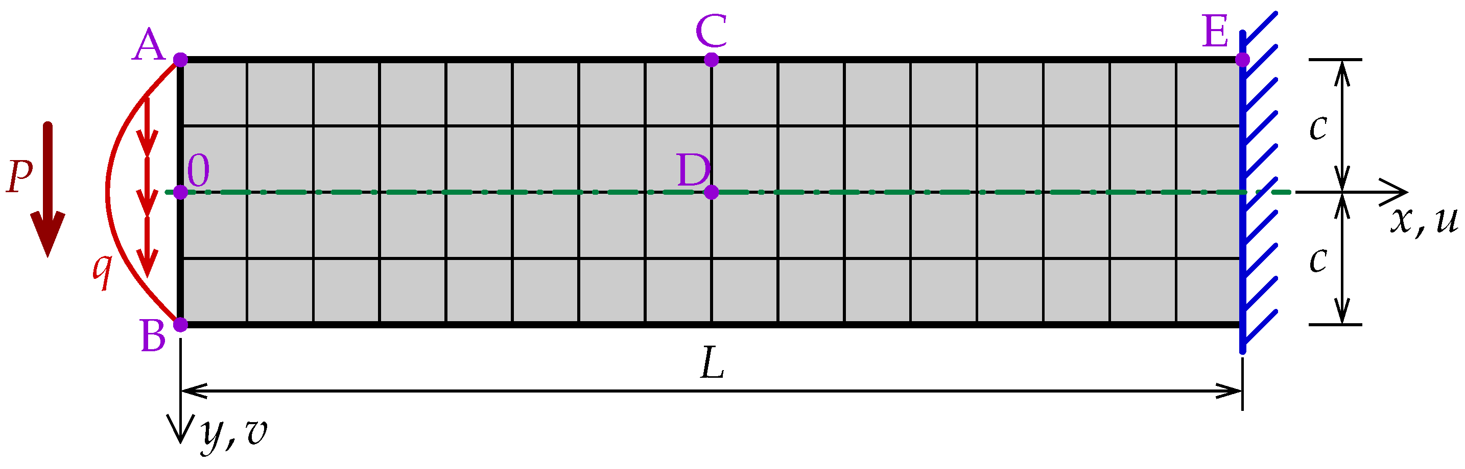Figure 1 depicts the specimen together with corresponding boundary conditions and additionally a discretization introduced by the medium mesh of quadrilateral (square) finite elements. On the left, a parabolic tangential load $q\left(y\right)$ is defined with a maximum value of $q_{\mathbf{max}}=500$ kN/m for point 0, i.e., for the origin of the coordinate system where $[x,y]=[0,0]$. After integration of the load, the resultant $P=40$ kN. On the right, a fixed (clamped) edge is set; however, according to the theoretical solution, two options of beam constraints can be regarded; see details, e.g., in [12]. For the first type, the effect of shear stresses is omitted, and it conforms with the Bernoulli–Euler theory. In the second case, the shear stresses are taken into account, so the Timoshenko–Ehrenfest theory [27,28] is valid. The data introduced in the computations are as follows: Young’s modulus is $E=200$ GPa, and Poisson’s ratio is $\nu =0.25$. The definition of the shear modulus is also needed according to the Timoshenko–Ehrenfest theory; hence, $G=80$ GPa. The length is $L=48$ cm, the height 12 cm corresponds to $2c$ in Figure 1, and the cantilever thickness is $b=1$ cm. The moment of inertia for the beam cross-section is $J_c=b{\left(2c\right)}^3/12=144$ cm⁴.

In this test, some characteristic quantities are monitored at points indicated in Figure 1. The definition of horizontal displacement $u\left(x,y\right)$ as well as vertical displacement $v\left(x,y\right)$, called also the beam deflection, is governed by the two aforementioned theories; see also [23]. According to the Bernoulli–Euler theory, on the clamped edge at point $[x,y]=[L,0]$, it is assumed that $\partial u/\partial y\ne 0$ and $\partial v/\partial x=0$, so the influence of shear stresses on the beam deflection is neglected. Based on the solution for this theory, the horizontal displacement is expressed as the function:

$$u^{\mathrm{B}–\mathrm{E}}\left(x,y\right)=-{\displaystyle \frac{P}{2E{J}_c}}{x}^{2}y+\left(-{\displaystyle \frac{\nu P}{6E{J}_c}}+{\displaystyle \frac{P}{6G{J}_c}}\right)y^3+\left({\displaystyle \frac{P{L}^2}{2E{J}_c}}-{\displaystyle \frac{P{c}^2}{2G{J}_c}}\right)y$$

(1)

The variable name is supplemented by upper index B–E. This displacement differs in sign depending on the y-coordinate, specifying points A and B, i.e., the corners on the left-hand side:

$$u^{\mathrm{B}–\mathrm{E}}\left(0,+c\right)=-u^{\mathrm{B}–\mathrm{E}}\left(0,-c\right)$$

(2)

Thereafter, in the computations, only positive horizontal translation given at point B is observed and referenced to the value, which for the above data equals:

$$u^{\mathrm{B}–\mathrm{E}}\left(0,+c\right)=-{\displaystyle \frac{\nu P{c}^3}{6E{J}_c}}+{\displaystyle \frac{P{L}^{2}c}{2E{J}_c}}-{\displaystyle \frac{P{c}^3}{3G{J}_c}}=0.09337\left[\mathrm{cm}\right]$$

(3)

The beam deflection, determined by the Bernoulli–Euler theory, is

$$v^{\mathrm{B}–\mathrm{E}}\left(x,y\right)={\displaystyle \frac{\nu P}{2E{J}_c}}{xy}^2+{\displaystyle \frac{P}{6E{J}_c}}{x}^3-{\displaystyle \frac{P{L}^2}{2E{J}_c}}x+{\displaystyle \frac{P{L}^3}{3E{J}_c}}$$

(4)

The maximum deflection given at point 0 is then equal to

$$v^{\mathrm{B}–\mathrm{E}}\left(0,0\right)={\displaystyle \frac{P{L}^3}{3E{J}_c}}=0.512\left[\mathrm{cm}\right]$$

(5)

When the Timoshenko–Ehrenfest theory is taken into account, the conditions $\partial u/\partial y=0$ and $\partial v/\partial x\ne 0$ hold for the clamped edge at point $[x,y]=[L,0]$, and the impact of shear stresses on the beam deflection is accounted for. Now, the horizontal displacement (upper index T–E is introduced) is derived as:

$$u^{\mathrm{T}–\mathrm{E}}\left(x,y\right)=-{\displaystyle \frac{P}{2E{J}_c}}{x}^{2}y+\left(-{\displaystyle \frac{\nu P}{6E{J}_c}}+{\displaystyle \frac{P}{6G{J}_c}}\right)y^3+{\displaystyle \frac{P{L}^2}{2E{J}_c}}y$$

(6)

The value of $u^{\mathrm{T}–\mathrm{E}}\left(0,+c\right)$ at point B is here calculated in this manner:

$$u^{\mathrm{T}–\mathrm{E}}\left(0,+c\right)=-{\displaystyle \frac{\nu P{c}^3}{6E{J}_c}}+{\displaystyle \frac{P{L}^{2}c}{2E{J}_c}}+{\displaystyle \frac{P{c}^3}{6G{J}_c}}=0.09712\left[\mathrm{cm}\right]$$

(7)

Analogically, the beam deflection in compliance with the Timoshenko–Ehrenfest theory can be obtained as a function and then determined at point 0 in the following way:

$$v^{\mathrm{T}–\mathrm{E}}\left(x,y\right)={\displaystyle \frac{\nu P}{2E{J}_c}}{xy}^2+{\displaystyle \frac{P}{6E{J}_c}}{x}^3-{\displaystyle \frac{P{L}^2}{2E{J}_c}}x+{\displaystyle \frac{P{L}^3}{3E{J}_c}}+{\displaystyle \frac{P{c}^2}{2G{J}_c}}(L-x)$$

(8)

$$v^{\mathrm{T}–\mathrm{E}}\left(0,0\right)={\displaystyle \frac{P{L}^3}{3E{J}_c}}+{\displaystyle \frac{PL{c}^2}{2G{J}_c}}=0.542\left[\mathrm{cm}\right]$$

(9)

The value $v^{\mathrm{T}–\mathrm{E}}\left(0,0\right)$ is $0.03$ cm larger than $v^{\mathrm{B}–\mathrm{E}}\left(0,0\right)$ due to the fact that the transverse shear effect of the beam is included in the solution according to the Timoshenko–Ehrenfest theory. The difference between the deflections according to the two theories can be estimated as

$$\Delta v\left(x,y\right)=v^{\mathrm{T}–\mathrm{E}}\left(x,y\right)-v^{\mathrm{B}–\mathrm{E}}\left(x,y\right)={\displaystyle \frac{P{c}^2}{2G{J}_c}}(L-x)=\Delta v\left(x\right)$$

(10)

The difference for the horizontal displacement can also be determined:

$$\Delta u\left(x,y\right)=u^{\mathrm{T}–\mathrm{E}}\left(x,y\right)-u^{\mathrm{B}–\mathrm{E}}\left(x,y\right)={\displaystyle \frac{P{c}^2}{2G{J}_c}}y=\Delta u\left(y\right)$$

(11)

Based on these differences, the following ratio $C_{\Delta }$ at point B can be defined:

$$C_{\Delta }={\displaystyle \frac{\Delta v}{\Delta u}}\left(0,+c\right)={\displaystyle \frac{L}{c}}$$

(12)

It is noticed that the ratio $C_{\Delta }$ corresponds to the simple geometric relation between L and c. The difference $\Delta u\left(0,+c\right)$ at point B equals $0.00375$ cm, so it is 8 times smaller than the difference $\Delta v\left(0,0\right)$ at point 0. Hence, it can be emphasized that for this configuration under in-plane bending, the transverse shear influences the deflection value at the free end. However, in the case of horizontal displacements at the corners of the free edge, its effect here is rather marginal. Moreover, $\Delta v\left(0,+c\right)$ at point B is also equal to $0.03$ cm. The quotient $L/c=8$ for such geometry, and therefore, the dimensions of the cantilever beam affect the proportion between the differences given in Equations (10) and (11). It can be recognized that the difference in Equation (11) comes from the last negative term in Equation (1) for the Bernoulli–Euler theory. Its absence in Equation (6) for the Timoshenko–Ehrenfest theory actually results in a larger value of the horizontal displacement $u^{\mathrm{T}–\mathrm{E}}\left(0,+c\right)$ in the comparison with $u^{\mathrm{B}–\mathrm{E}}\left(0,+c\right)$ for the Bernoulli–Euler theory. All the translation values calculated above, based on both theories, serve as a basis for comparison with the displacements obtained in the numerical analysis.

Apart from the above functions, the stress field for this cantilever beam can be defined:

$${\sigma }_x\left(x,y\right)=-{\displaystyle \frac{Pxy}{J_c}},{\sigma }_y\left(x,y\right)=0,{\tau }_{xy}\left(x,y\right)=-{\displaystyle \frac{P}{2J_c}}\left(c^2-y^2\right)$$

(13)

and can be observed at selected points of the specimen. Normal stress ${\sigma }_x\left(x,y\right)$ along the extreme lower and upper edges $y=\pm c$ is given as

$${\sigma }_x\left(x,\pm c\right)=\mp {\displaystyle \frac{Pxc}{J_c}}$$

(14)

Consequently, based on the applied data, the following values of ${\sigma }_x$ are obtained in the middle of the beam (where $x=L/2$) and on the clamped edge (where $x=L$):

$${\sigma }_x\left({\displaystyle \frac{L}{2}},\pm c\right)=\mp 400\left[\mathrm{MPa}\right],{\sigma }_x\left(L,\pm c\right)=\mp 800\left[\mathrm{MPa}\right]$$

(15)

These are values of normal stress at points C and E in Figure 1, and they are used for comparison during the computations. Similarly to the load function $q\left(y\right)$, tangential stress ${\tau }_{xy}$ also has a parabolic character along the height, and its minimum is attained on axis $y=0$:

$${\tau }_{xy}(x,0)=-{\displaystyle \frac{P{c}^2}{2J_c}}=-50\left[\mathrm{MPa}\right]$$

(16)

The absolute value $|{\tau }_{xy}(x,0)|$ at the center of the beam, i.e., at point D in Figure 1, is taken into account for further comparisons.

As mentioned in the introduction, the numerical analysis is carried out using two engineering programs: Midas [10] and Robot [9]. Similar computations for the cantilever beam using various types of FEs, for example, programmed by the author of [17], are conducted in his paper. Five different densities in the finite element discretization are applied in order to perform the convergence study. Starting from the coarsest mesh with the finite element size equal to 12 cm and division $4\times 1$ for squares, each next mesh is four times denser, so the finest mesh has the FE size of $0.75$ cm and division $64\times 16$ for squares. Moreover, meshes with only square FEs, i.e., quadrilaterals Q4 with four nodes or with only triangular FEs T3 with three nodes, are considered. The equivalent nodal load is recalculated for each mesh by the authors using their own subroutine. Together with a given shape of FE its structural type is also significant since the choice of both these features affects the usage of a particular FE, included in the software. In Midas, different kinds of structures are available, and among others, a membrane or a shell can be selected for this example. Surprisingly, it turns out that both options provide the same results. However, if the membrane structure is chosen, an additional variant is accessible, namely extra DOFs, given here as drilling rotations, that can be activated. The influence of drilling rotations on the results is shown below. The details of the formulation, as well as the implementation of FE with these enhancing DOFs, can be found in many papers, e.g., [15,16,17,29,30,31]. When the choice of the structure type is set as a membrane or a shell for the computations in Robot, the results differ as expected. The convergence study is accordingly conducted for cases summarized in

Table 1. List of finite elements applied in cantilever test.

	Applied	Applied Finite Element
Abbreviation	Program	Shape	Type	Option
M-Q4dr	Midas	Quadrilateral Q4	Membrane	Drilling rotations
R-Q4sh	Robot	Quadrilateral Q4	Shell
M-Q4	Midas	Quadrilateral Q4	Membrane
R-Q4m	Robot	Quadrilateral Q4	Membrane
M-T3dr	Midas	Triangle T3	Membrane	Drilling rotations
M-T3	Midas	Triangle T3	Membrane
R-Q4sh	Robot	Triangle T3	Shell
R-Q4m	Robot	Triangle T3	Membrane

. The abbreviations listed in the table are prepared for better readability of the diagrams illustrated in Figure 2, Figure 3, Figure 4, Figure 5 and Figure 6.

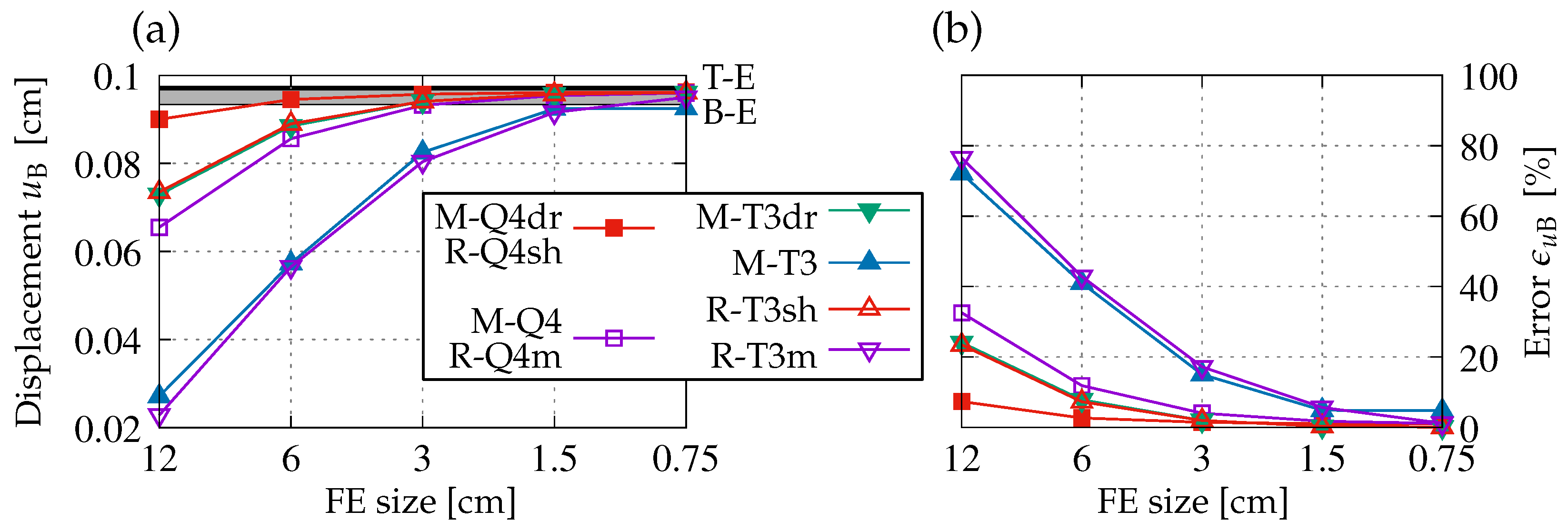
Figure 2 is composed of two images where horizontal displacement $u\left(0,+c\right)$, called here $u_{\mathrm{B}}$, is investigated, considering numerical solutions from both programs. The framed legend is correlated with Table 1 and the set in Figure 2 between these images. It should also be mentioned that linetypes and markers defined in the legend are the same for the next figures. A variable on the abscissa axis is the FE size, which changes with the log scale, so all presented diagrams show the dependence on discretization from the coarsest mesh to the finest one. On the left-hand side, the values of displacement $u_{\mathrm{B}}$ are depicted directly. The thin black solid line refers to $u^{\mathrm{B}–\mathrm{E}}\left(0,+c\right)$ in Equation (3), according to the Bernoulli–Euler theory. The thick black solid line indicates $u^{\mathrm{T}–\mathrm{E}}\left(0,+c\right)$ in Equation (7) as the upper limit of computed horizontal displacement values, based on the Timoshenko–Ehrenfest theory. Additionally, a gray band between these lines is distinguished, which can be interpreted as a zone of theoretical values. On the right-hand side, the relative error ${ϵ}_{u\mathrm{B}}$ calculated for the numerical values referenced to analytical $u^{\mathrm{T}–\mathrm{E}}\left(0,+c\right)=0.09712$ cm is exemplified. Firstly, it is noticed that the results for cases M-T3 (blue line with filled triangles) and R-T3m (purple line with blank inverted triangles) are poor for coarse and medium meshes. There are responses for discretizations with FEs known as constant strain triangles (CST), where standard bilinear shape functions are implemented. On the other hand, $u_{\mathrm{B}}$ for cases M-Q4dr and R-Q4sh is the best, so the smallest error ${ϵ}_{u\mathrm{B}}$ is visible for them, even if the coarse mesh is used in the computations. Moreover, both of them have two identical numerical values for each corresponding mesh, so they are marked as one red line with filled squares. A similar coincidence as for the aforenamed cases with quadrilaterals Q4 can also be seen for cases with triangle elements T3. Despite the fact that the displacements for corresponding meshes are not exactly the same, the diagrams for cases M-T3dr (green line with filled inverted triangles) and R-T3sh (red line with blank triangles) overlap almost perfectly. It can be concluded that when in-plane bending is analyzed, membrane FEs in Midas with active drilling rotations behave very similarly to shell FEs in Robot. As expected, it is shown that the values of displacement $u_{\mathrm{B}}$ and the relative error determined for them in all cases with triangle meshes reveal lower accuracy. However, for both types of FEs, quadratic convergence is attained as the mesh is refined. Analogically to M-Q4dr and R-Q4sh, the results for cases M-Q4 and R-Q4m are numerically twinned, so again, only one diagram is plotted (the purple line with blank squares). These responses for displacement $u_{\mathrm{B}}$ on the left and the relative error on the right are given for solutions with classic four-noded FEs (Q4) without any enhancements. For coarser meshes, especially with triangular FEs, it is observed that the presence of drilling rotations in the finite element interpolation improves the solution.

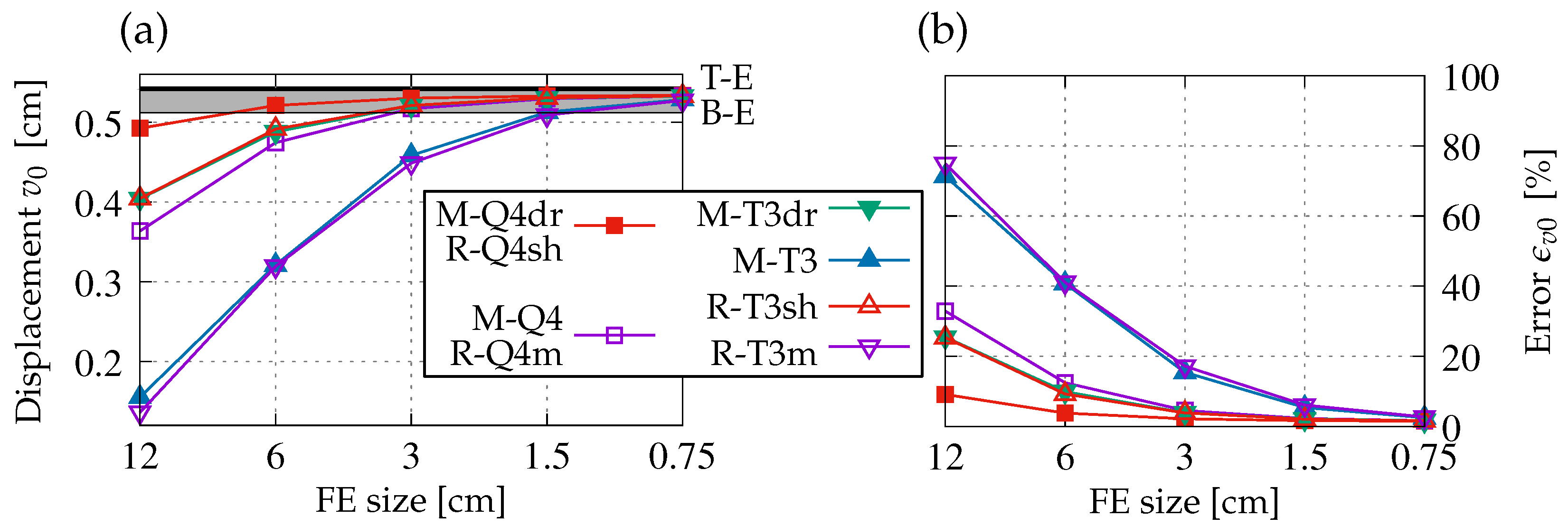
Figure 3 illustrates the results observed at point 0. Values of vertical translation, also interpreted as the beam deflection and marked by $v_0$, are represented on the left. Numerical solutions are confronted with the theory, similar to the analysis discussed in Figure 2. Here, the thin black solid line corresponds to the value $v^{\mathrm{B}–\mathrm{E}}\left(0,0\right)$ given in Equation (5) for the Bernoulli–Euler theory, while the thick black solid line conforms to the value $v^{\mathrm{T}–\mathrm{E}}\left(0,0\right)$ determined in Equation (9) according to the Timoshenko–Ehrenfest theory. Similarly to Figure 2, a gray zone between the lines is apparent in Figure 3, creating an interval based on both theories as a reference for values $v_0$. On the right-hand side in Figure 3, the relative error ${ϵ}_{v0}$ is reproduced, but here in regard to $v^{\mathrm{T}–\mathrm{E}}\left(0,0\right)=0.542$ cm. Generally, it can be stated that all comments that describe the results given in Figure 2 are also valid for the current results. Similarities and analogies between respective cases are the same. One can only add that displacement $v_0$ for cases M-Q4dr and R-Q4sh are within the zone of analytical solutions when the square mesh with FE size 6 cm or denser is applied. On the contrary, the numerical value of $v_0$ for M-T3 and R-T3m with triangular FEs is within this zone only when the size $0.75$ cm is introduced. Based on the results presented in Figure 2 and Figure 3, it can also be concluded that displacements converge from below in this benchmark.

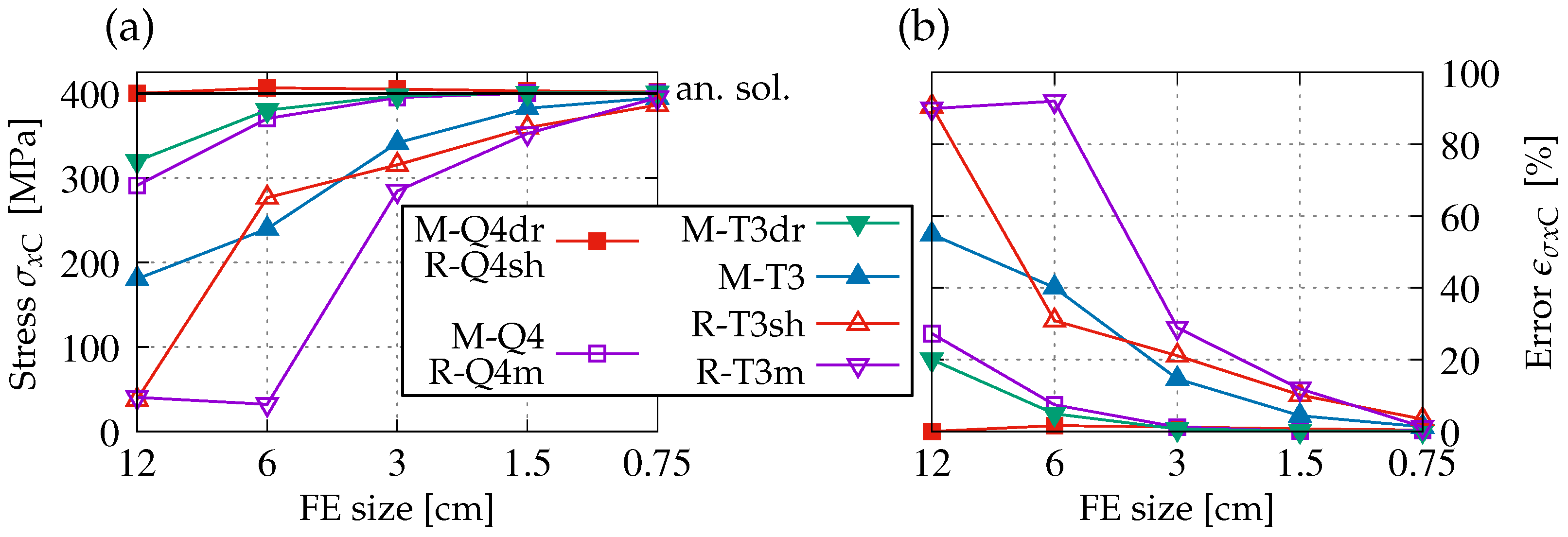
The results for stresses are shown in Figure 4, Figure 5 and Figure 6. The method of presentation and description for subsequent cases is the same as previously. Figure 4 refers to the normal stress ${\sigma }_x$ observed at point C, so it is called here ${\sigma }_{x\mathrm{C}}$. The exact value comes from Equation (15) and equals ${\sigma }_x\left(L/2,-c\right)=400$ MPa. It also provides the reference to estimate the relative error ${ϵ}_{\sigma x\mathrm{C}}$. The stress values, together with their counterparts of the error, show that the meshes made of triangular FEs, i.e., M-T3, R-T3sh, and R-T3m, provide deficient responses. The exception is the finest mesh. Only the results for case M-T3dr, when drilling rotations are activated in Midas, can be treated as satisfactory. On the other hand, if Q4 FEs are applied, the values of stress ${\sigma }_{x\mathrm{C}}$ are much closer to the analytical solution. However, the error in the results in the case of M-Q4 and R-Q4m for the coarsest mesh exceeds 25%.

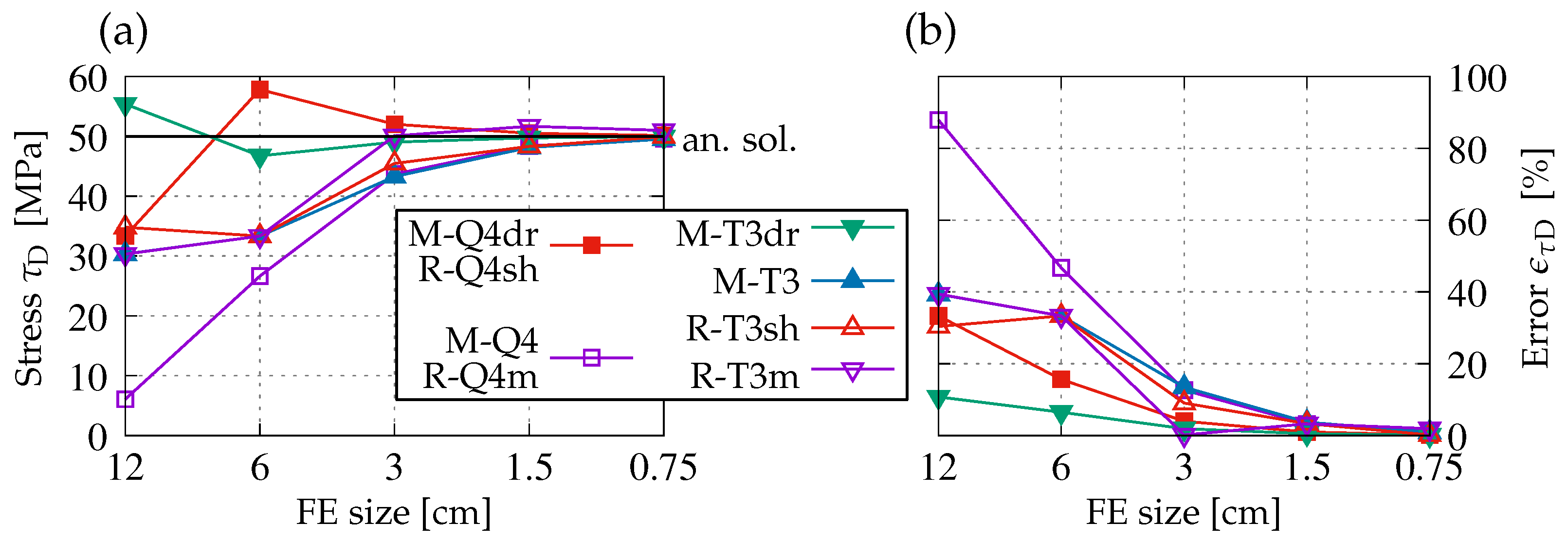
In the next figure, Figure 5, the attention is focused on tangential stress ${\tau }_{xy}$ at point D, called here shortly ${\tau }_{\mathrm{D}}$. The absolute value $|{\tau }_{xy}(L/2,0)|=50$ MPa connected with Equation (16) is taken as the analytical solution to assess the relative error ${ϵ}_{\tau \mathrm{D}}$. Now the poorest results are noticed for cases M-Q4 and R-Q4m if the computations are performed with coarse or medium meshes. On the other hand, the values of stress ${\tau }_{\mathrm{D}}$ for M-Q4dr, R-Q4sh, and M-T3dr are nearest to the theoretical 50 MPa. It is also seen for these cases that convergence is attained pretty quickly. Summarizing all the results for displacements and stresses obtained so far, it can be stated that, using coarse meshes, the values are more or less underestimated. Of course, this is related to the shear locking effect for membranes, which occurs for poor discretizations and when the displacement field as the primary one is interpolated in FEs in the most conventional way.

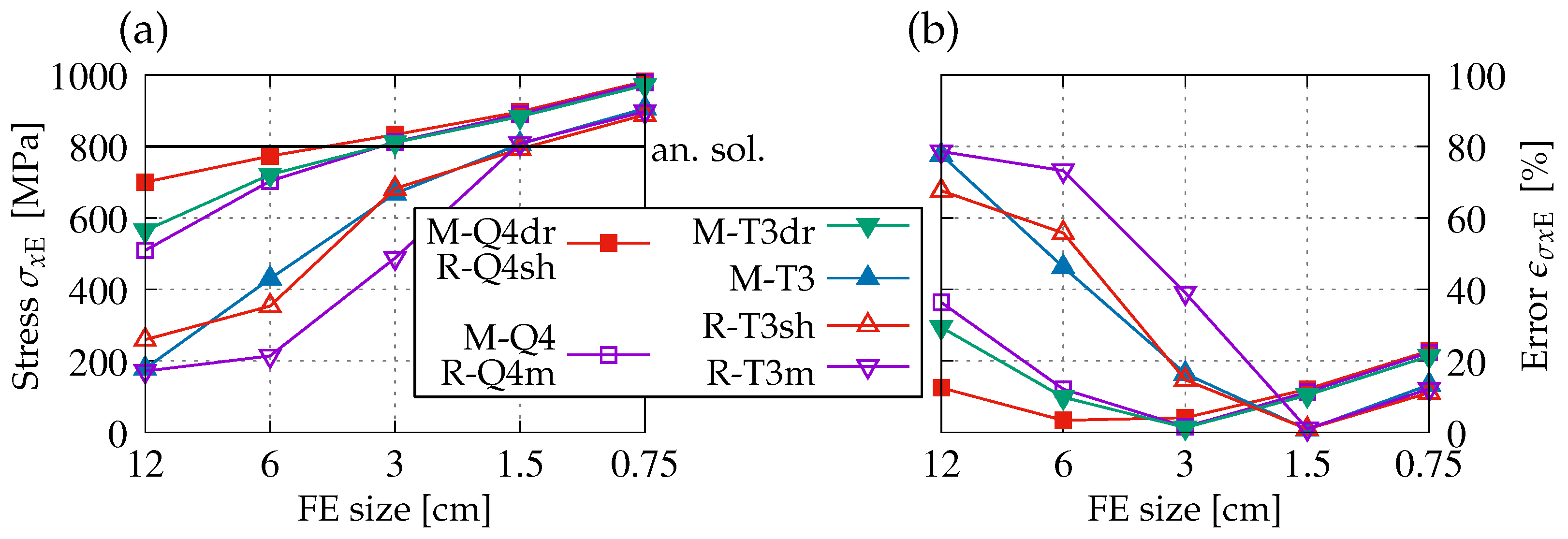
Figure 6 depicts the values of normal stress ${\sigma }_x\left(L,-c\right)$ at point E, which is called ${\sigma }_{x\mathrm{E}}$, and their associated relative errors ${ϵ}_{\sigma x\mathrm{E}}$. The tendency for successive meshes seems to be similar to ${\sigma }_{x\mathrm{C}}$. Stress values ${\sigma }_{x\mathrm{E}}$ for M-T3, R-T3sh, and R-T3m in the case of a coarse mesh are strongly underestimated, while for M-T3dr and for the solutions with FEs Q4, this underestimation is less pronounced and decreases quickly. However, the values of ${\sigma }_{x\mathrm{E}}$ for the two finest meshes exceed the theoretical value of 800 MPa determined in Equation (6). Moreover, it is visible that relative errors ${ϵ}_{\sigma x\mathrm{E}}$ are larger for the mesh with FE size $0.75$ cm than for the mesh with FE size $1.5$ cm. It should be noted that point E is located at the corner of the specimen on the fixed edge. A tendency towards infinite stress with mesh refinement is detected in such regions during numerical analyses, which is also in accordance with the classical elasticity theory. In other words, the value of stress ${\sigma }_{x\mathrm{E}}$ can grow and grow when discretization becomes increasingly dense. This phenomenon is known as stress singularity; see [18,19,32]. From a physical point of view, stress concentration can occur in areas with geometric or material discontinuity, and it destroys the results of simulations with fine discretization. Moreover, the stress field is extrapolated from integration points that are located inside FEs, and this can additionally amplify the increase in stress values at such corners. Due to this fact, the convergence study or the search for maximum stress in the singularity region cannot lead to an objective estimation. Here, point E is selected deliberately to show that performing a convergence study does not make sense for certain locations. Furthermore, a so-called root singularity pattern, shown as a contour plot in [17], confirms that the highest intensity of the stress field arises exactly at corners near the clamped edge.

The issue of stress singularities is extensively discussed in [33]. In FEM, special singular elements and a measure called the stress intensity factor can be introduced; see [34]. The method of analytical constraints associated with FEM can be employed. If possible, the concentrated loadings and nodal supports should be avoided in FE modeling by introducing geometric punches or imposing multi-point constraints. The issue of the fixed corner in the elastic range cannot be completely eliminated, but various techniques can be introduced to address it, as for example a superconvergent patch recovery method [35]. A review of various approaches is presented in detail in [18]. Another solution is to extend the analysis beyond the elastic range. In the plasticity theory, the stress concentration effect is reduced by material yielding. However, different smoothing techniques can still be applied in nonlinear analyses, such as a discontinuous smoothing recovery method combined with an adaptive calculation scheme [36] for elastoplastic problems. If a crack or localization occurs in the numerical analysis, various averaging methods can be adopted, providing regularization by means of different localization limiters [37], among others, gradient terms. Moreover, the gradients as the averaging factors can be present in elasticity [38] or even via the standard Fourier’s law in thermoplasticity [39]. An alternative approach used in fracture analysis can be phase-field modeling, where a sharp crack is replaced by a so-called diffusive crack zone [40]. The combination of phase-field and strain gradient models to overcome the stress singularity problem is shown in [41]. To summarize, to avoid this issue in simulations, various smoothing techniques, at the post-processing stage but not only, can be included. In the next section, the bending moment reduction, as an available option in Robot and Midas, for the values derived from the solutions in the slab-column connection is shown.

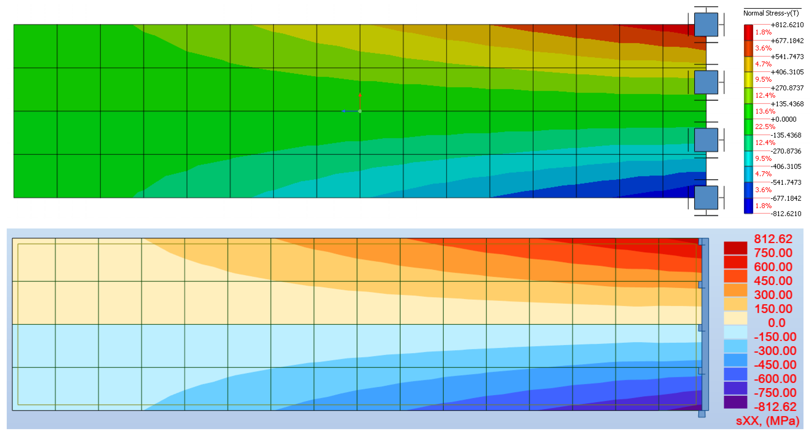
Figure 7 illustrates contour plots of stress ${\sigma }_x$ for the medium mesh from computations in Midas and Robot. Both distributions are almost identical.

Based on the presented results, it can be concluded that membrane FEs available in both Midas and Robot packages behave alike and provide almost the same solution for corresponding meshes. During FEM analysis, the activation of drilling rotations for membranes in Midas corresponds to the use of shell FEs in Robot. However, FEs with standard bilinear interpolation for plane stress problems are the default in both packages.

3. Bending of Slab Supported by Column

In FEM models for slab (as well as shell) structures, the bending moment values obtained at points of discrete supports or connections with columns may be overestimated. These locations are referred to as stress concentration points. The slab’s bending moment values increase significantly with mesh refinement. Consequently, they become unreliable for further use, such as in reinforcement design for slabs. This effect can be mitigated by a reduction in moments at the support or column. The objective of this benchmark is to demonstrate the impact of applying a reduction in the post-processing stage on the slab’s bending moments at the column connection. Both Midas and Robot software provide this functionality, albeit in different ways. The results of this reduction in the two programs are compared. Additionally, in Robot, the influence of the column’s cross-sectional dimensions on the reduction measure is considered, i.e., the change in the values of the slab’s bending moment after reduction is studied. In Midas, the reduction domain is directly defined by a certain characteristic distance, and this has also been verified. The ability to adopt a force and moment reduction above columns and walls as well as above nodal and linear supports is crucial. Proper usage of the reduction option for forces and moments at these connection points is beneficial.

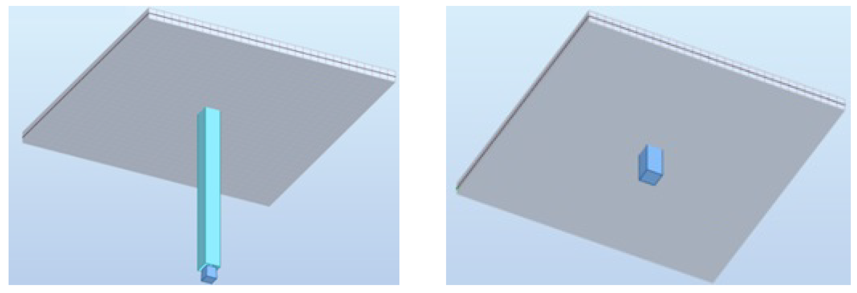
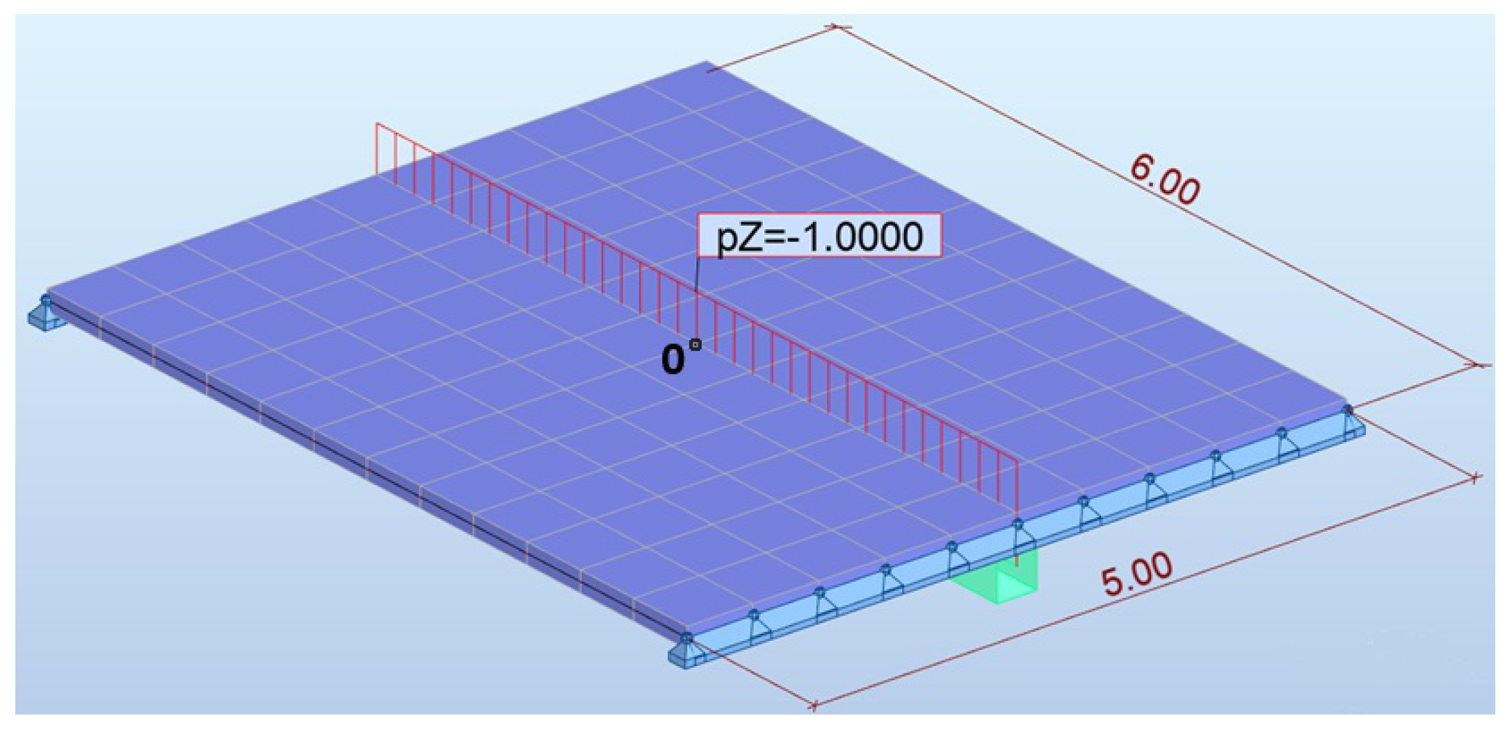
As the benchmark in this section, the simplest possible model of the connection between the slab and the column has been created. Out-of-plane bending is now studied. The slab is square and supported by the column in the center; see Figure 8. Such geometry indicates that there are four symmetry axes: two along the edges and two along the diagonals. The model could, therefore, be limited to a quarter, but it is intentionally considered for the entire domain to verify whether the symmetry is correctly reproduced. Moreover, a seemingly simple configuration may provoke difficulties during computations due to single-node support and/or discrepancies between the FE dimensions of the slab and the column, which can lead to an ill-conditioned system of equations. Square FEs with a corresponding approximation for out-of-plane bending are applied in both computational programs [9,10]. The span of the slab is $L=4.96$ m, and its thickness is $d=20$ cm. The dimensions of the column are as follows: the height is $H=3$ m, and the edge size of the square cross-section is $b=30$ cm. For both the slab and the column, concrete C30/37 is assumed, with the following material properties: Young’s modulus is $E=33$ GPa, Poisson’s ratio is $\nu =0.2$, and shear modulus is $G=13.333$ GPa. The surface transverse load ${\widehat{q}}_z=2$ kN/m², uniformly distributed on the whole slab, is applied.

The model of the entire configuration can be constructed in two ways. The column is fully represented as a structural element or can be replaced by a fixed nodal support, whereby the column edge size is defined to enable moment reduction. Figure 8 illustrates both options. The computations in Midas are carried out with the full representation of the slab and column. The computations in Robot are performed with the assumption that the support with the additionally specified size at the node corresponds to the full model. The validity of adopting this simplification in Robot is explained below. 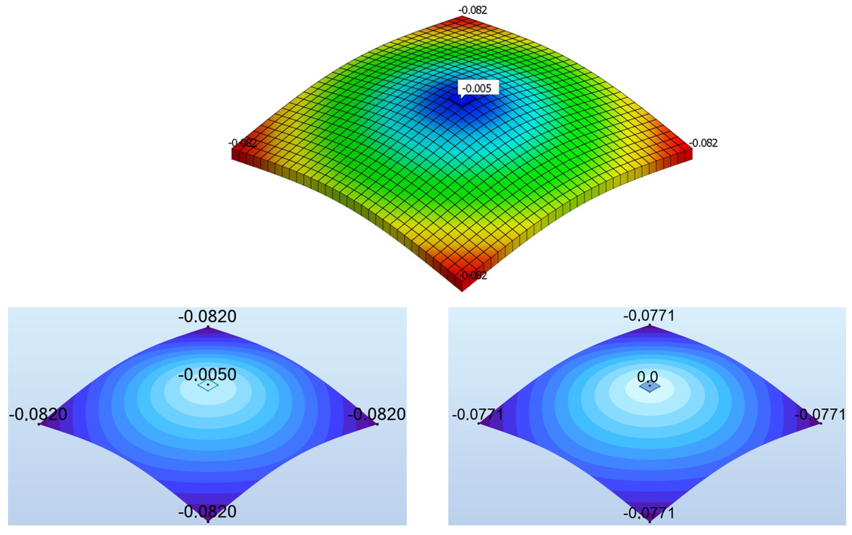Figure 9 shows the deformations of the slab obtained in both packages. It is visible that the symmetry is obeyed. At the top, the solution from Midas is depicted. The mesh with $32\times 32$ elements is employed for the slab, i.e., the FE size equals $h_{\mathrm{FE}}=15.5$ cm. At the bottom, the results from Robot are demonstrated. The same discretization is adopted. On the left, there is the deformation for the model of the slab and full column. On the right, the counterpart with the nodal support is presented. The numbers in the subfigures of Figure 9 represent the deflection of the slab at the center and at all corners. When the column is introduced into the model, the deflection of $-0.005$ cm is observed in the center. The column is actually very slightly shortened (compressed). When the full model is considered, the deflections in Midas (at the top) and in Robot (at the bottom on the left) are identical. It is noted that both packages are equipped with an implementation of so-called discrete Kirchhoff–Mindlin quadrilateral (DKMQ) FEs; see [14]. The difference between the central value and extreme deflections at corners equals $0.0770$ cm. If the nodal support is assumed, as shown in Figure 9 at the bottom on the right, obviously, the central deflection equals zero. The difference in the deflection between the center and corners is now $0.0771$ cm, which is almost identical to the full version of the model. It could, therefore, be presumed that both variants of the model are equivalent. Hence, the option with the nodal support can be adopted for the next analysis in Robot.

It should also be mentioned that during the computations in Robot a so-called instability occurs in both types of the model, indicating the connection point as the cause of this perturbation. Global extremes of the displacement field should be verified in that case. If any excessively large values are noticed in the results, the model should be improved. Global displacement extremes in this benchmark do not produce unexpected results; consequently, the warning related to instability can be ignored. The computations in Midas do not involve any problems despite the challenging configuration of the model from a numerical solution perspective.

Before displaying further results, one aspect arising from the theory should be mentioned. If this problem were reduced to the bending of a one-dimensional cantilever beam with a length equal to half the slab’s span, by calculating the sum of the surface load from the entire slab’s span to a resultant uniform load along the beam’s axis $q_s={\widehat{q}}_{z}L=9.92$ kN/m, then the value of the fixed-end moment for such a cantilever with length $L/2$ is

$$M_{\mathrm{f}}=0.5q_s{(L/2)}^2=30.506\left[\mathrm{kNm}\right]$$

(17)

This value of $M_{\mathrm{f}}$ is consistent here with the integral $I_{mxx}$ determined from the slab’s bending moments along the centerline $x=0$:

$$I_{mxx}={\int }_{-2.48}^{2.48}{m}_{xx}\mathrm{d}y$$

(18)

Firstly, attention is focused on analyzing the bending moments for the slab depending on the mesh density, based on the solutions computed only in the Robot program.

Table 2. Influence of discretization on moment reduction in slab above column—results from Robot.

Division	FE Size	Without Reduction		With Reduction
$\mathit{N}\mathbf{\times }\mathit{N}$	${\mathit{h}}_{\mathbf{FE}}$	$\mathbf{max}{\mathit{m}}_{\mathit{xx}}$	${\mathit{I}}_{\mathit{mxx}}$	$\mathbf{max}{\mathit{m}}_{\mathit{xx}}$	${\mathit{I}}_{\mathit{mxx}}$
	[cm]	[kNm/m]	[kNm]	[kNm/m]	[kNm]
$8\times 8$	62	16.501	30.559	7.437	24.970
$16\times 16$	31	20.804	30.570	10.445	27.392
$32\times 32$	15.5	25.128	30.555	11.591	27.760
$64\times 64$	7.75	28.873	30.534	11.933	28.315
$128\times 128$	3.875	32.274	30.521	11.934	28.338
$256\times 256$	1.9375	35.569	30.513	12.327	28.518

shows the following in the respective columns: mesh division $N\times N$, the size of square FE $h_{\mathrm{FE}}$, and the results when the reduction option is turned off or on. In each case, the maximum value of the bending moment $m_{xx}$ together with the value of the corresponding integral $I_{mxx}$ is listed. When the moment reduction above the support is not enabled, the maximum values of $m_{xx}$ increase with the mesh density. This moment for the finest mesh is more than double that for the coarsest mesh. Such a rise is solely related to the mesh refinement pitfall and can lead to incorrect interpretation of the results. On the other hand, the values of the integral $I_{mxx}$ converge to the theoretical value $M_{\mathrm{f}}$, ranging from $30.599$ kNm to $30.513$ kNm. When the reduction option is activated, moments $m_{xx}$ for the refined discretizations tend to be more or less 12 kNm/m, except in the case of the coarsest mesh, where the value of $m_{xx}$ is underestimated. The integral $I_{mxx}$, along with the consecutive solutions, approaches the value of about $28.5$ kNm. This is approximately 2 kNm less than the integral determined for the case of $256\times 256$ elements without the use of reduction. The difference will be clarified by the following description of Figure 10, Figure 11 and Figure 12.

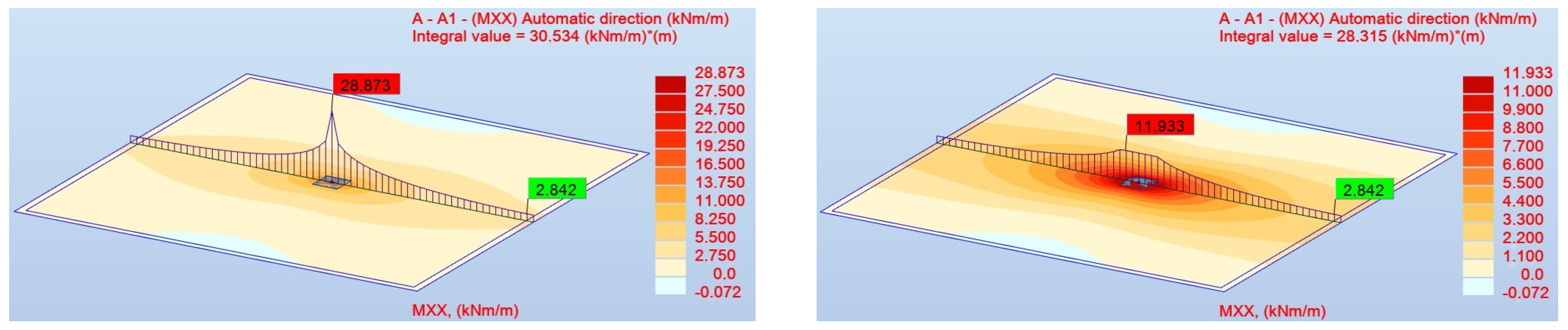
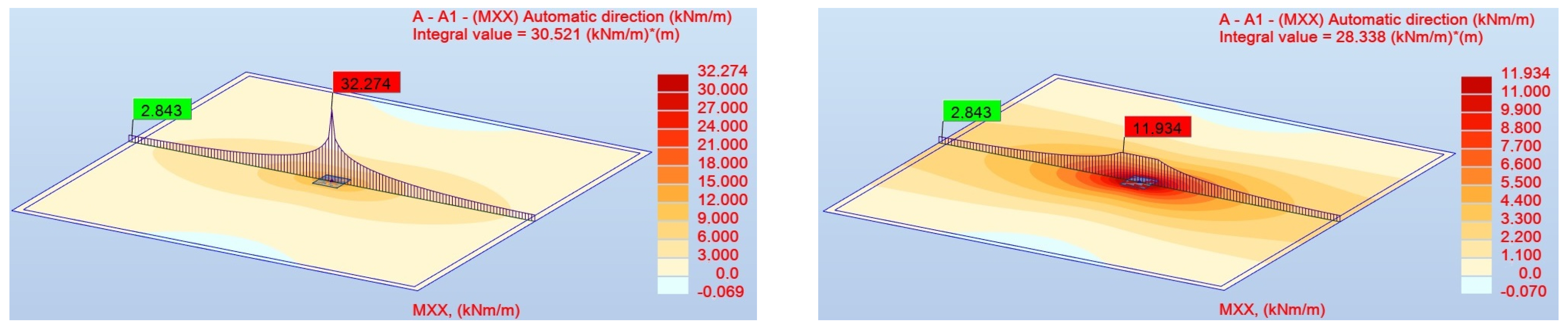
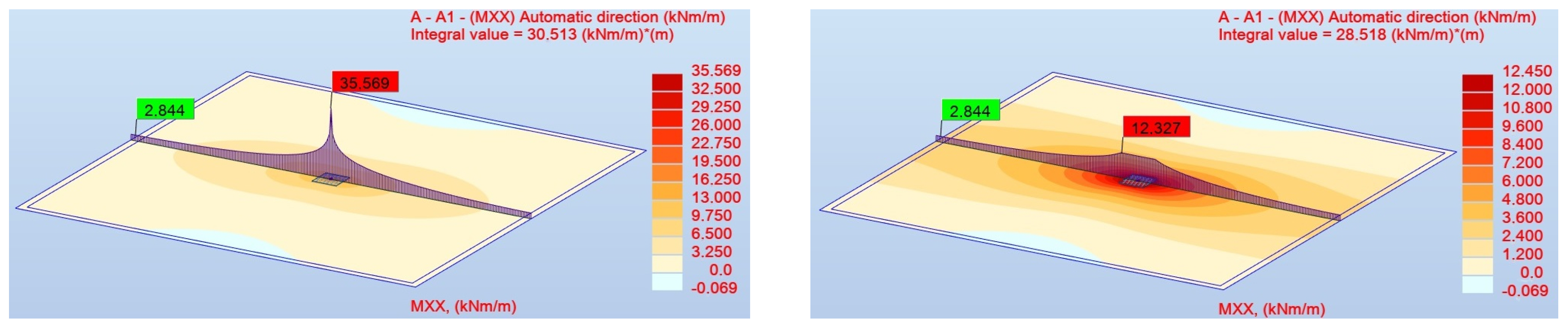
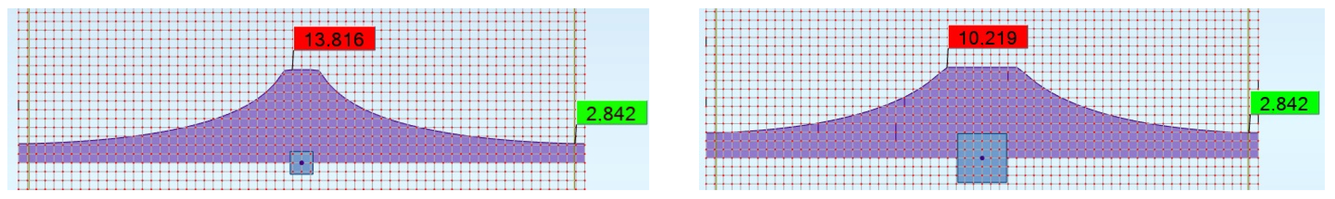
Figure 10, Figure 11 and Figure 12 illustrate bending moments $m_{xx}$ using both panel cut diagrams and contour plots. On the left-hand side, the original results, i.e., without the reduction, are presented. On the right-hand side, the reduction is employed during post-processing to represent the moments $m_{xx}$ more adequately. The distributions for the last three finest meshes are shown. These figures confirm the numerical results listed in Table 2. Looking at the functions of $m_{xx}$ for panel cuts, their character is similar for each mesh, respectively, for the unmodified results on the left and then for the results on the right when the reduction is applied. The maximum clearly grows with mesh density for the original results on the left. The distribution of contour plots is strongly localized above the column. The ones on the right are limited due to the introduced reduction. The patterns with the applied reduction have a more diffuse character, and the color gradient adjusts according to the scale. The panel cut for reduced moments looks truncated by the presence of the defined column size (here $b=30$ cm). The introduction of such a limitation actually makes the results objective. Additionally, in the top right corner of the figures, the integral values for each case are shown. If a reduction is activated, the function of $m_{xx}$ is limited, so the values of $I_{mxx}$ are also lowered.

The next aspect of the analysis focuses on the influence of the column size on the reduction in the slab’s bending moments. The computations are carried out in Robot using the same mesh $64\times 64$ with $h_{\mathrm{FE}}=7.75$ cm. The maximum value of $m_{xx}$ is $28.873$ kNm/m and corresponds to $I_{mxx}=30.534$ kNm if the results are not corrected. Of course, these results are independent of the column size.

Table 3. Influence of column size on reduced bending moments $m_{xx}$ in slab center, results for Robot and mesh with 64 FEs alongside.

Size of column	[cm]	20	22–24	26–32	34	36–42	44
Moment  ${\mathit{m}}_{\mathit{xx}}$	[kNm/m]	13.816	12.720	11.933	11.320	10.600	10.219
Integral  ${\mathit{I}}_{\mathit{mxx}}$	[kNm]	29.014	28.620	28.315	28.002	27.612	27.361

shows the reduction effect when the size of the column is changed. Here, both the moment $m_{xx}$ and the integral $I_{mxx}$ decrease as the column size increases. The ranges that are distinguished in the first row of the table refer to discrete values. For example, the same reduction degree is recognized for the column size of 26 cm as well as 32 cm. The bold values are also correct for initial $b=30$ cm, so they coincide with the distributions displayed in Figure 10. Figure 13 presents the diagrams of the bending moments $m_{xx}$ in the slab panel cuts for two extreme cases of the applied column size: the smallest, 20 cm, and the largest 44, cm. It is observed that the reduction region of the moment $m_{xx}$ is derived from the column size.

The idea of determining the reduction zone in Robot to limit the values of $m_{xx}$ around the column is illustrated in Figure 14. The method is demonstrated for the mesh with square FEs and different column cross sections. First, the reduction radius is evaluated based on half of the diagonal of the column’s cross-section. Then, the nodes and the centers (here marked in yellow) of FEs that are inside the circle are selected. The primary bending moment values are replaced with the reduced ones at all these points. The interiors of the light pink areas limited by the red lines are subjected to this reduction. The extreme (maximum or minimum) of the bending moment is found among the values at the nodes marked in orange. For example, in the drawings in Figure 14, this refers to the node highlighted additionally in cyan. Finally, such a value is imposed on the reduction area.

In the Midas program, during the calculation stage, there is no option to directly adopt reduction. Therefore, to apply the reduction in the model, the slab reinforcement has to be predefined. Arbitrarily, the entire slab is designed with $⌀10$ reinforcement bars spaced at 20 cm at the bottom and $⌀10$ bars spaced at 10 cm at the top, in both directions, x and y. The concrete cover is equal to 3 cm. It should be emphasized that, in this configuration, the upper layer of the slab is subjected to tension. Of course, now the reinforced slab has greater stiffness. After computations, there are two modes available for reviewing the results in the Midas interface: static analysis or dimensioning. In the post-processing stage, the reduction option operates only in the dimensioning mode.

Table 4. Influence of discretization on moment reduction in slab above column—results from Midas.

		No	Reinforcement: Reduction via Parameter W
Division	FE Size	Reinforcement	$\mathit{W}\mathbf{=}\mathbf{0}$ cm	$\mathit{W}\mathbf{=}\mathbf{50}$ cm	$\mathit{W}\mathbf{=}\mathbf{150}$ cm
$\mathit{N}\times \mathit{N}$	${\mathit{h}}_{\mathbf{FE}}$	$\mathbf{max}{\mathit{m}}_{\mathit{xx}}$	$\mathbf{max}{\mathit{m}}_{\mathit{xx}}$	$\mathbf{max}{\mathit{m}}_{\mathit{xx}}$	$\mathbf{max}{\mathit{m}}_{\mathit{xx}}$
	[cm]	[kNm/m]	[kNm/m]	[kNm/m]	[kNm/m]
$8\times 8$	62	8.88	11.99	11.99	10.32
$16\times 16$	31	12.22	16.50	16.50	11.39
$32\times 32$	15.5	15.60	17.11	11.99	9.41
$64\times 64$	7.75	18.93	17.89	12.64	9.30
$128\times 128$	3.875	22.21	18.40	12.83	9.29
$256\times 256$	1.9375	25.48

presents the influence of mesh division on the slab’s moment reduction in Midas. The third column of numbers shows the maximum $m_{xx}$ values for the slab without rebars and, thus, also without reduction. Similarly to the results for Robot in Table 2, these values increase with mesh densification. The results for the same slab, but with the reinforcement, are presented in subsequent columns. The reduction distance from the column axis should be specified for the RC slab, and here, it will be referred to as width W. The bending moments are presented for the cases $W=0$ cm, $W=50$ cm, and 150 cm, respectively. Blank cells in Table 4 for $256\times 256$ FEs indicate that these computations could not be completed for the finest mesh due to sudden interruptions, even after restarting the task from the beginning. Nevertheless, activating the reduction via the given width leads to a decrease in the moment $m_{xx}$ at the slab-column connection. For the reduction option with $W=50$ cm and 150 cm, each successive mesh refinement tends to a specific value of the slab’s bending moment. For $W=50$ cm, the moment $m_{xx}$ eventually exceeds $12.5$ kNm/m, while for $W=150$ cm, it approaches approximately $9.3$ kNm/m. When the larger parameter W is used, the moments are underestimated. However, it should be noted that in this case, the reduction option activates starting from the coarsest mesh with $8\times 8$ FEs. For smaller $W=50$ cm, it becomes effective for $32\times 32$ FEs or denser meshes. Meshes with 8 and 16 FEs along the edge are too coarse to trigger a moment reduction for this distance.

Table 5. Influence of reduction distance W on bending moments $m_{xx}$ at slab center, results for Midas and mesh with 64 FEs alongside.

Reduction width W	[cm]	0	15	25	50	75	100	150
Moment   ${\mathit{m}}_{\mathit{xx}}$	[kNm/m]	17.89	15.70	13.95	12.64	11.34	10.32	9.30

indicates the effect of the reduction width on the bending moment value in Midas. Now, only one mesh with 64 FEs along the edge is employed while W grows. As expected, similarly to the dependence on the column size in Robot as shown in Table 3, the value of the reduced bending moment for the slab decreases as parameter W increases. The most suitable choice seems to be distance $W=50$ cm or 75 cm. For both cases, $m_{xx}$ after reduction is close to 12 kNm/m, agreeing reasonably well with the case of $b=30$ cm in Robot. The reduced moment $m_{xx}=9.30$ kNm/m for $W=150$ cm is clearly underestimated, which corresponds to the exaggeratedly large reduction area; see Figure 15.

The reduction in Midas works as a weighted average method. The original value of $m_{xx}$ is recalculated at the central node, selected due to the connection of the slab to the column and in its defined vicinity. First, this vicinity is specified as a square area with a width W. All FEs within this region, i.e., given by the size $W/2$ in horizontal left and right as well as vertical up and down, are taken into account. It concerns internal and contiguous elements restricted to the square. The bending moments are computed by extrapolation from integration points at each node of a given FE. These values belong to each separate element. The final value at the central node is then averaged based on nodal values but derived from patch FE functions. Moreover, weighting factors, which depend on the distances between the central node and sequentially considered nodes, affect this averaging operation. Thus, the determined bending moment $m_{xx}$ is assigned to all nodes within the zone defined by the given width W.

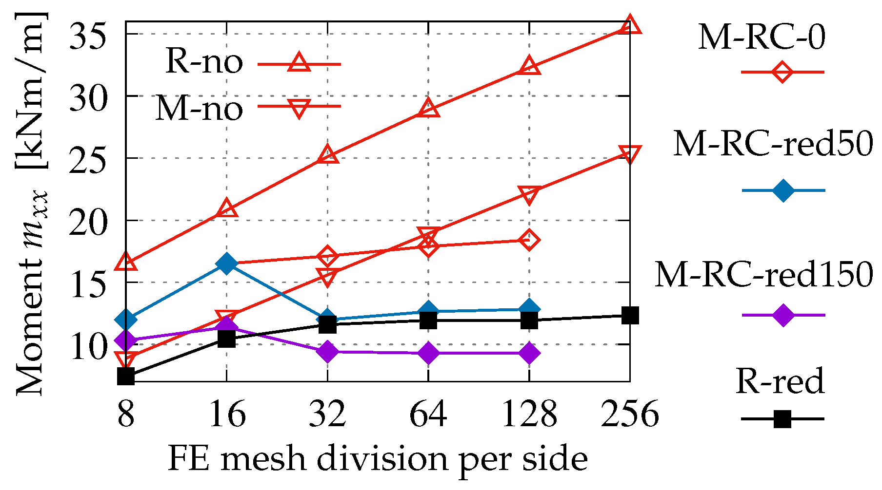
The last part of this section summarizes the entire analysis discussed above. The abbreviations listed in

Table 6. Types of moment reduction in slab supported by column illustrated in Figure 16.

Abbreviation	Applied Program	If Reduction	Column Size $\mathit{b}$ [cm]	Reduction Width $\mathit{W}$ [cm]
R-no	Robot	No	30
M-no	Midas	No	30
M-RC-0	Midas	No	30
M-RC-red50	Midas	Yes	30	50
M-RC-red150	Midas	Yes	30	150
R-red	Robot	Yes	30

are useful for understanding Figure 16. This figure concisely highlights the key aspects of this study. Each case in Figure 16 represents the diagram of moments $m_{xx}$ at the center of the slab as a function of FE density from the coarsest to the finest mesh. The abscissa axis changes in the logarithmic scale. The cases R-no and M-no refer to the original results in Robot and Midas, respectively, i.e., without any reduction in the post-processing stage. They are marked by red lines with empty triangles, straight and inverted, respectively. It is noticed that both diagrams grow almost linearly, but the R-no for Robot starts from a larger value. M-RC-0 is connected with the case for Midas, where the rebars are introduced into the slab model, but the reduction does not work ($W=0$ cm). The diagram for this case also increases with mesh densification, although the rate of growth is much slower than for R-no and M-no. The case M-RC-red50 corresponds to width $W=50$ cm for the reduction in the slab moments in Midas. The reduction effect for this width starts from the third mesh. In fact, the results for $8\times 8$ and $16\times 16$ FEs are identical to those for M-RC-0. The values of $m_{xx}$ are limited for subsequent meshes, as shown in the diagram with a blue line and filled diamonds. Next, the diagram marked by a purple line and filled diamonds is given for M-RC-red150 with distance $R=150$ cm. Its character is similar to the previous one, but now, all bending moments are underestimated. The case R-red, marked by a black line and filled squares, involves the reduction activation in Robot based on the column size. When the results are observed for discretizations $32\times 32$, $64\times 64$, and $128\times 128$, cases R-red and M-RC-red50 are quite close to each other. This demonstrates that the reduction effect can be successfully activated in both Robot and Midas packages and can give similar results.

4. Interaction of Beam with Slab

The third benchmark concerns the analysis of out-of-plane bending based on the model of a slab, which is in interaction with a beam. The configuration is presented in Figure 17. The slab has length $L_x=6.0$ m, width $L_y=5.0$ m, and thickness $d=15$ cm. The beam span is $L_x=6.0$ m, and it has a rectangular cross-section of $b\times h=30.0\times 40.0$ cm. Both structural elements are made of concrete C30/37, with material properties as in the previous section: Young’s modulus is $E=33$ GPa, Poisson’s ratio is $\nu =0.2$, and shear modulus is $G=13.333$ GPa. The edges of the slab along the width ($L_y=5.0$ m) are simply supported, i.e., translations are constrained. Uniformly distributed load $p_Z=1$ kN/m is applied along the beam, as shown in Figure 17. For the computations in both packages, two meshes consisting of rectangular FEs are employed: a coarser mesh with FEs $1.25\times 1.20$ m and a finer mesh with FEs $0.5\times 0.5$ m. A similar study, but much more concise, performed only on Robot and for a concrete slab with a steel beam, was demonstrated in [42].

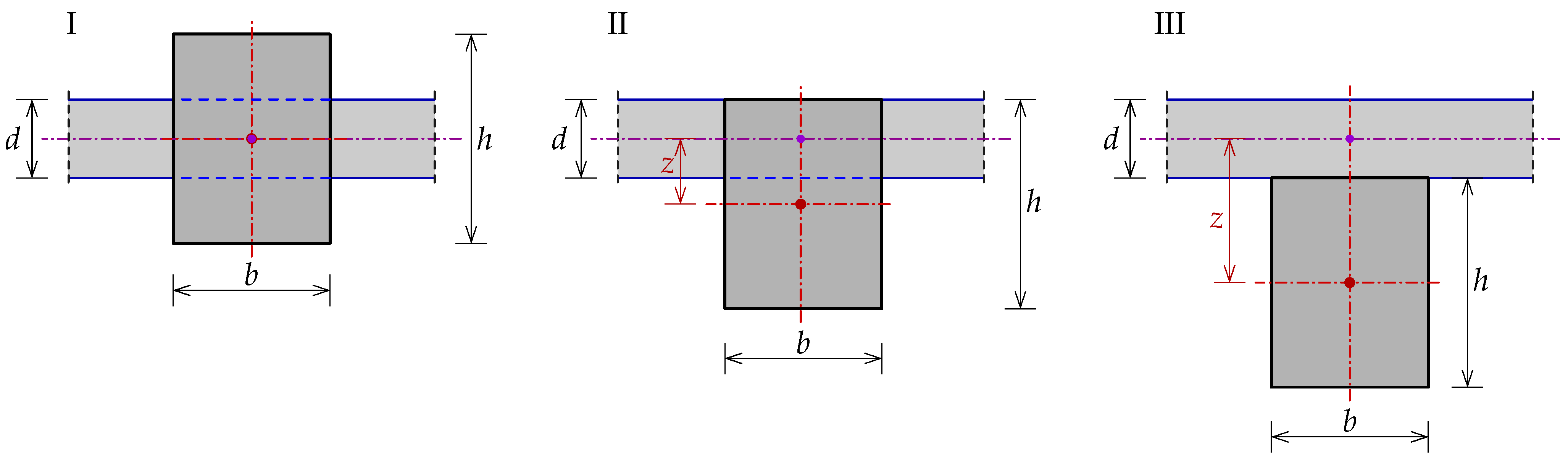
There are three variants of the connection between the beam and the slab, as depicted in Figure 18. The simplest version of the model, marked with the Roman numeral I, occurs when the beam axis aligns with the middle plane of the slab, i.e., no offset exists and $z=z_{\mathrm{I}}=0$ cm. The second type of connection, marked by II, assumes that the upper flange of the beam coincides with the top plane of the slab, so the offset corresponds to $z=z_{\mathrm{II}}=12.5$ cm. The last case of connection is presented in Figure 18 on the right-hand side and marked by III. Here, the upper beam flange faces the bottom plane of the slab, and the offset is $z=z_{\mathrm{III}}=27.5$ cm. The study and comparison of these specified connections are described later in the section.

Now, before discussing the aforementioned versions of the model and their results, the first aspect of the analysis is to determine whether the offset definition causes any changes in the obtained values. The study focuses only on type II connection with $z=z_{\mathrm{II}}=12.5$ cm. Various options available in Robot for modeling connectors between the beam and the slab are investigated:

(a)

Directly using the function offset;

(b)

Activating so-called rigid links for all nodes along the beam and their corresponding nodes of the slab;

(c)

Shifting down the beam by the distance $z=12.5$ cm and inserting very stiff and stable members between the nodes of the beam and their counterparts on the slab.

These members are artificially defined as round short pipe rods with high stiffness ($E=300$ MPa and $\nu =0.3$) and an extremely large section: diameter $d_p=1219.0$ mm and ring thickness $t_w=25.0$ mm, leading to a cross-sectional area of $A_p=$ 93,776.54 mm². The results obtained using the three options listed above are consistent with each other. The offset function, rigid links, or connector members form a particular type of frame. As a result, additional axial forces $F_x$ are generated in the beam, along with bending moments $M_y$. These axial forces occur due to the presence of offsets, specified in different ways, and the creation of a frame structure consisting of beam FEs and the connector members linking the beam to the slab as short studs. The bending moment $M_y$ and axial force $F_x$ diagrams are presented in Figure 19 for case II(b) as an example. The remaining options (a) and (c) exhibit almost the same distributions of $M_y$ and $F_x$. Additionally, the equilibrium of selected beam nodes has been verified for case (c), thanks to which the formation of the frame and axial forces has been confirmed. This entire analysis proves that the offset function effectively acts as a rigid link between the beam and the slab. As a result, all three aforementioned options are equivalent. Moreover, non-zero axial forces in that case become apparent. The character of both $M_y$ and $F_x$ diagrams is discontinuous, and jumps are governed by the lengths of beam FEs. The presence of axial forces, when the offset option is used, must be considered in calculating the final value of the bending moment for the beam. In further computations, case (a) will be used, and at a later stage of the study, it will be denoted by the suffix “-o”.

The beam in this benchmark, cooperating with the slab, provides the function of bending moments $M_y\left(x\right)$ as for a simply supported beam. Therefore, the theoretical value of $M_y$ for the beam can be determined. The extreme point is located at point 0, where $x=L_x/2=3$ m (see Figure 17), and the moment equals:

$$M_y^0=0.125p_Z{L_x}^2=4.50\left[\mathrm{kNm}\right]$$

(19)

When deriving the total bending moment $M_y^{\mathrm{\Sigma }}$ for a beam interacting with the slab, considering the offset effect, three components should be taken into account:

$$M_y^{\mathrm{\Sigma }}=M_y+F_{x}z+I_{mxx}^{\mathrm{s}}$$

(20)

Maximum values of the bending moment $M_y$ and the axial force $F_x$ (absolute value) at midpoint 0 are read from the beam diagrams, as in case II(b), where they are highlighted in the boxes in Figure 19. The integral $I_{mxx}^{\mathrm{s}}$ is determined based on the panel cut perpendicular to the beam so that slab bending moment $m_{xx}$ along the y-axis is summed:

$$I_{mxx}^{\mathrm{s}}={\int }_0^{L_y}{m}_{xx}\mathrm{d}y$$

(21)

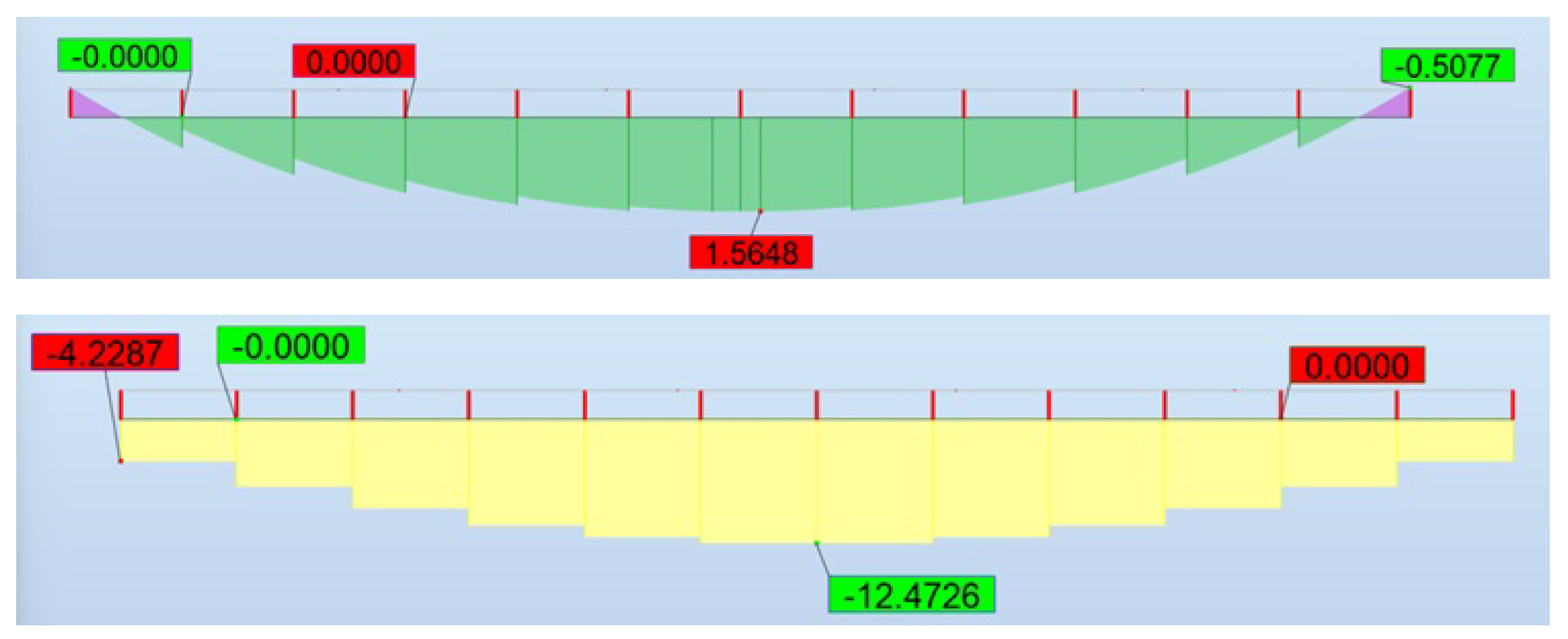
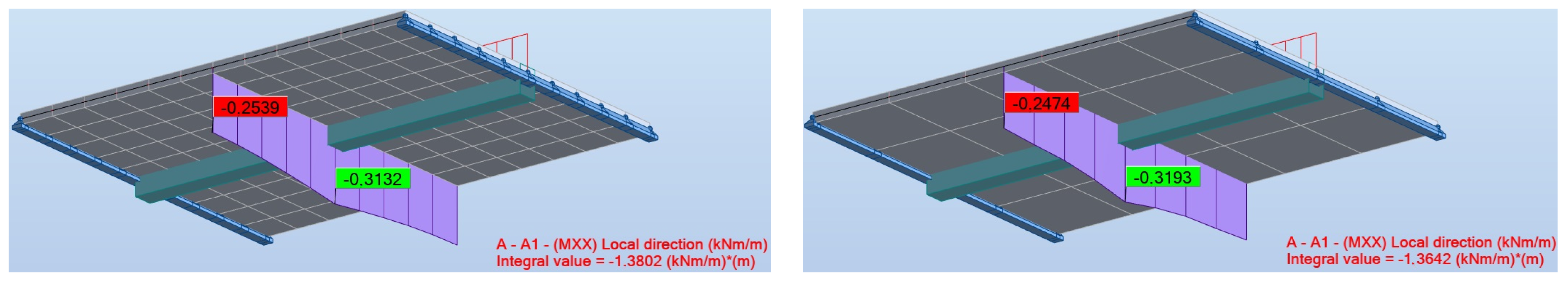
The panel cuts of $m_{xx}$ along width $L_y$ (in the middle of length $L_x$) are illustrated in Figure 20 for the computations carried out in Robot using two meshes. In addition, the respective integral values $I_{mxx}^{\mathrm{s}}$ are shown as well. Figure 20 also depicts the schemes of the model, FE meshes for both densities, supports along width $L_y$, and the position of load $p_Z$ is visible as well. For example, the total value of the bending moment $M_y^{\mathrm{\Sigma }}$ at midpoint 0 is then calculated for the finer mesh as

$$M_y^{\mathrm{\Sigma }}=1.5648+12.4726·0.125+1.3802=4.5041\left[\mathrm{kNm}\right]$$

(22)

This arithmetic takes into account the appropriate absolute values based on the results obtained in Robot.

In the Midas program, it is not possible to read the value of the integral $I_{mxx}^{\mathrm{s}}$ directly for a given panel cut. Hence, to assess it, the values of the slab’s bending moments $m_{xx}$ along an indicated intersection can be taken into account. After that, a numerical method such as the trapezoidal rule can be applied to derive $I_{mxx}^{\mathrm{s}}$. The results for the model in Midas with offset type II and the finer mesh are presented in Figure 21 and Figure 22. 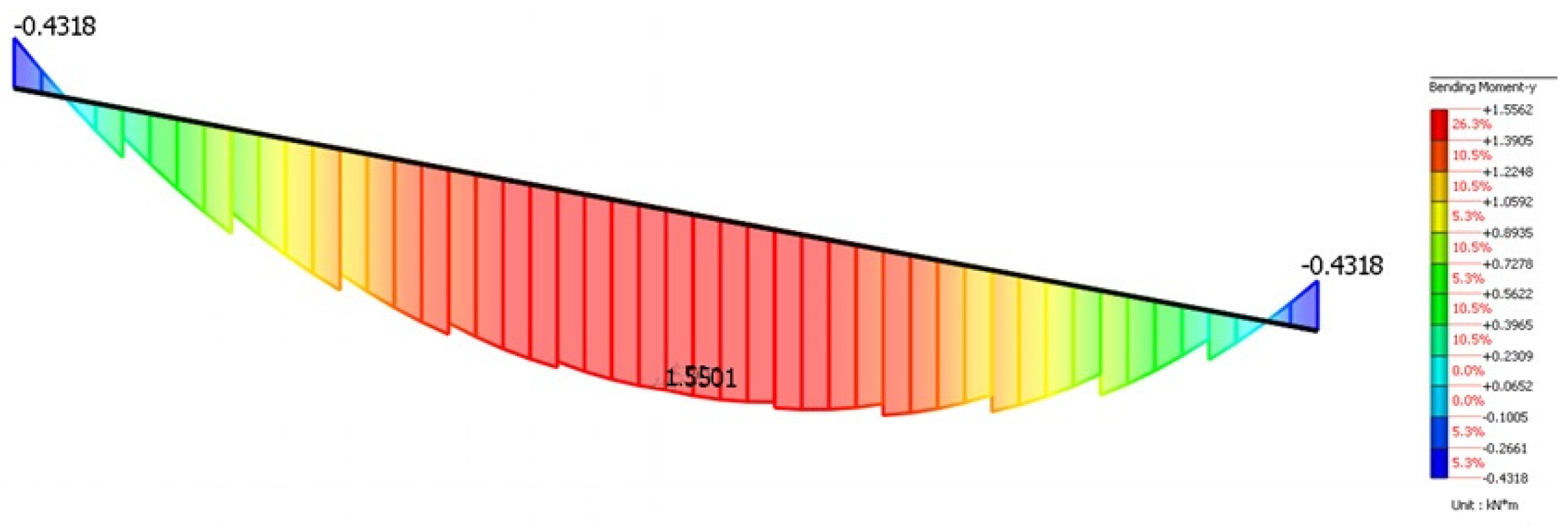Figure 21 visualizes the diagram of $M_y$ for the beam. As for the diagrams from Robot, given in Figure 19, the jumps between values are observed due to its discretization into FEs with specific lengths. 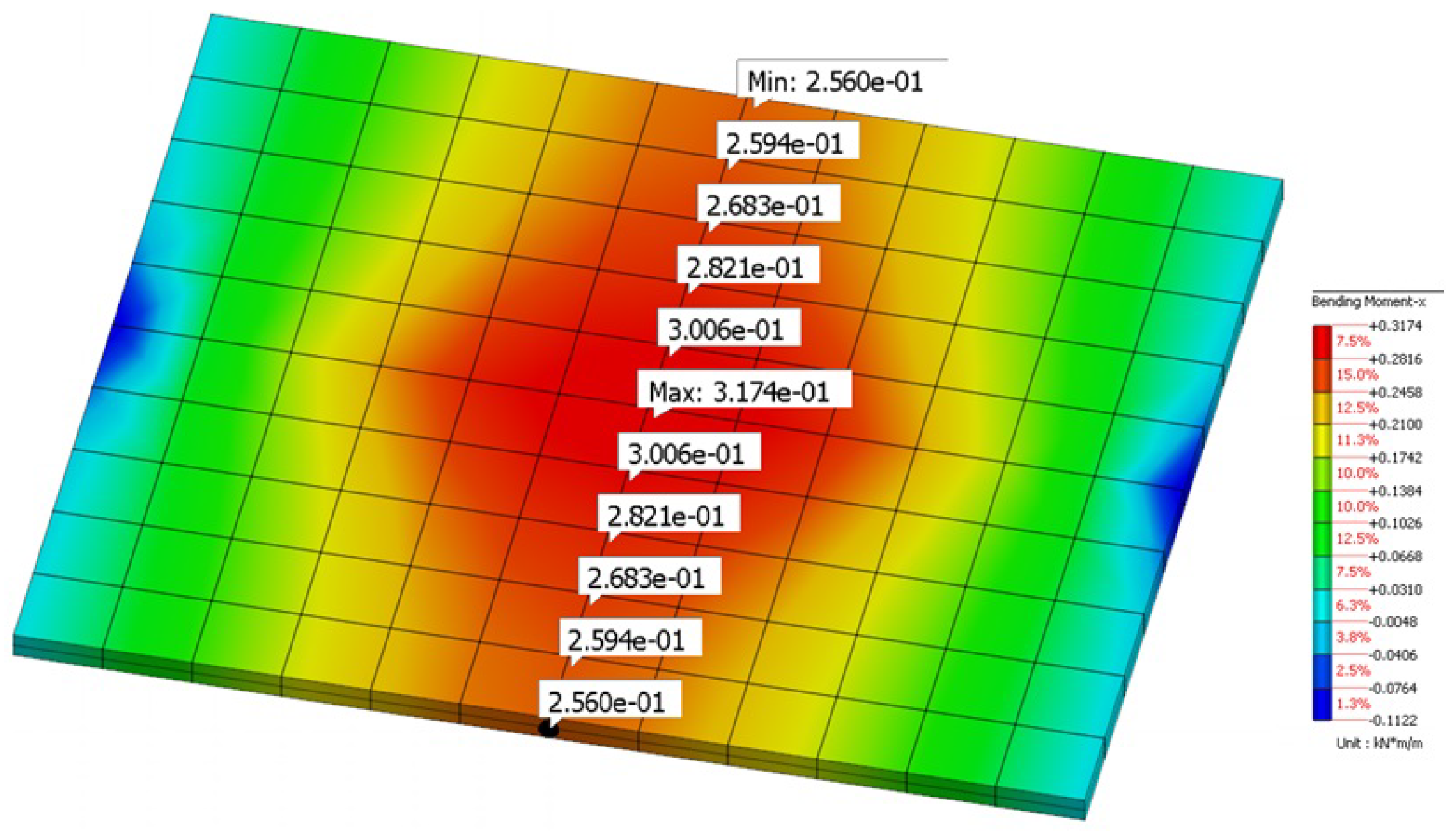Figure 22 displays a contour plot of bending moments $m_{xx}$ for the slab. Together with this distribution, the values of $m_{xx}$ along the width $L_y$ at midpoint 0 are distinguished. They are needed to determine $I_{mxx}^{\mathrm{s}}$ by the trapezoidal rule. After this integration, the total value of the moment $M_y^{\mathrm{\Sigma }}$ for the Midas computations, using type II and the finer mesh, equals:

$$M_y^{\mathrm{\Sigma }}=1.5501+12.4228·0.125+1.3971=4.5000\left[\mathrm{kNm}\right]$$

(23)

An alternative approach to operating with the offset in the model is to preserve the beam–slab configuration in the basic form, as defined in option I (see Figure 18), and then appropriately modify the value of the moment of inertia for the beam. Its initial value is

$${J_y}^{\mathrm{I}}={\displaystyle \frac{b{h}^3}{12}}=1.60·{10}^{-3}{[\mathrm{m}}^4]$$

(24)

Adopting the parallel axis theorem, the moments of inertia for connection type II with $z_{\mathrm{II}}=12.5$ cm and type III with $z_{\mathrm{III}}=27.5$ cm are calculated, respectively, as follows:

$${J_y}^{\mathrm{II}}={\displaystyle \frac{b{h}^3}{12}}+bh{z_{\mathrm{II}}}^2=3.475·{10}^{-3}{[\mathrm{m}}^4]$$

(25)

$${J_y}^{\mathrm{III}}={\displaystyle \frac{b{h}^3}{12}}+bh{z_{\mathrm{III}}}^2=10.675·{10}^{-3}{[\mathrm{m}}^4]$$

(26)

In Midas, such adjusted geometric characteristics have to be directly input into the beam data. The Robot software tool requires the entry of the so-called section’s moment of inertia coefficient depending on the distance z. For configurations II and III, these entries are determined by the ratio:

$$C_{\mathrm{II}}={\displaystyle \frac{{J_y}^{\mathrm{II}}}{{J_y}^{\mathrm{I}}}}=2.171875,C_{\mathrm{III}}={\displaystyle \frac{{J_y}^{\mathrm{III}}}{{J_y}^{\mathrm{I}}}}=6.671875$$

(27)

The coefficient C is originally given to account for the cracking of a section, and in that case, it is usually reduced for the beam analysis. However, here it is regarded to indicate the position of the beam related to the slab as for the offset option. Note that both modified values of the moment of inertia, directly as in Midas or by means of C as in Robot, are also transferred to the next software modules for dimensioning. The total bending moment $M_y^{\mathrm{\Sigma }}$ is still calculated using Equation (20), but according to connection type I, where $z=z_{\mathrm{I}}=0$ cm, the second term vanishes. This approach, where the beam’s moment of inertia is updated, is further denoted by suffix “-m”.

The bending moment $M_y^{\mathrm{\Sigma }}$ and its particular components are determined at the beam mid-span for each connection type, either by using the offset option or by considering the moment of inertia.

Table 7. Summary of results from Robot.

Connection Type	z [cm]	Mesh	${\mathit{M}}_{\mathit{y}}$ [kNm]	${\mathit{F}}_{\mathit{x}}$ [kN]	${\mathit{M}}_{\mathit{y}}+{\mathit{F}}_{\mathit{x}}\mathit{z}$ [kNm]	${\mathit{I}}_{\mathit{mxx}}^{\mathbf{s}}$ [kNm]	${\mathit{M}}_{\mathit{y}}^{\mathbf{\Sigma }}$ [kNm]	${\mathit{w}}_0$ [mm]
I	0	Finer	$2.375$	$0.0$	$2.375$	$2.126$	$4.501$	$0.1707$
II-o	$12.5$	Finer	$1.565$	$12.473$	$3.124$	$1.380$	$4.504$	$0.1094$
II-m	$12.5$	Finer	$3.190$	$0.0$	$3.190$	$1.310$	$4.500$	$0.1050$
III-o	$27.5$	Finer	$0.696$	$11.642$	$3.898$	$0.603$	$4.501$	$0.0477$
III-m	$27.5$	Finer	$3.971$	$0.0$	$3.971$	$0.529$	$4.500$	$0.0424$
I	0	Coarser	$2.415$	$0.0$	$2.415$	$2.084$	$4.499$	$0.1710$
II-o	$12.5$	Coarser	$1.586$	$12.430$	$3.140$	$1.364$	$4.504$	$0.1108$
II-m	$12.5$	Coarser	$3.217$	$0.0$	$3.217$	$1.283$	$4.500$	$0.1001$
III-o	$27.5$	Coarser	$0.714$	$11.502$	$3.877$	$0.636$	$4.513$	$0.0493$
III-m	$27.5$	Coarser	$3.982$	$0.0$	$3.982$	$0.518$	$4.500$	$0.0404$

shows the results for Robot, while

Table 8. Summary of results from Midas.

Connection Type	z [cm]	Mesh	${\mathit{M}}_{\mathit{y}}$ [kNm]	${\mathit{F}}_{\mathit{x}}$ [kN]	${\mathit{M}}_{\mathit{y}}+{\mathit{F}}_{\mathit{x}}\mathit{z}$ [kNm]	${\mathit{I}}_{\mathit{mxx}}^{\mathbf{s}}$ [kNm]	${\mathit{M}}_{\mathit{y}}^{\mathbf{\Sigma }}$ [kNm]	${\mathit{w}}_0$ [mm]
I	0	Finer	$2.364$	$0.0$	$2.364$	$2.137$	$4.501$	$0.1716$
II-o	$12.5$	Finer	$1.550$	$12.423$	$3.103$	$1.397$	$4.500$	$0.1107$
II-m	$12.5$	Finer	$3.167$	$0.0$	$3.167$	$1.333$	$4.500$	$0.1068$
III-o	$27.5$	Finer	$0.685$	$11.592$	$3.873$	$0.627$	$4.500$	$0.0491$
III-m	$27.5$	Finer	$3.942$	$0.0$	$3.942$	$0.558$	$4.500$	$0.0448$
I	0	Coarser	$2.407$	$0.0$	$2.407$	$2.100$	$4.507$	$0.1636$
II-o	$12.5$	Coarser	$1.589$	$12.424$	$3.142$	$1.405$	$4.547$	$0.1062$
II-m	$12.5$	Coarser	$3.202$	$0.0$	$3.202$	$1.320$	$4.522$	$0.1018$
III-o	$27.5$	Coarser	$0.720$	$11.582$	$3.905$	$0.698$	$4.603$	$0.0488$
III-m	$27.5$	Coarser	$3.969$	$0.0$	$3.969$	$0.584$	$4.553$	$0.0427$

shows the results for Midas. The following columns are specified: the connection type, the distance z, mesh density, the moment $M_y$, and the axial force $F_x$ read from the diagram; their combination $M_y+F_{x}z$; the integral $I_{mxx}^{\mathrm{s}}$ from the panel cut, the total value $M_y^{\mathrm{\Sigma }}$, and additionally the deflection $w_0$ at point 0 (Figure 17). The suffix “-o” or “-m” refers to how the position of the beam relative to the slab is taken into account. It is evident in the cases with non-zero offset (“-o”) that the force $F_x$ has to be included in calculating $M_y^{\mathrm{\Sigma }}$. Generally, the values of this total bending moment correspond to the theoretical $M_y^0=4.5$ kNm. The results for the coarser mesh are less accurate, especially in Midas, where the integrals $I_{mxx}^{\mathrm{s}}$ are estimated using the trapezoidal rule along the panel cut, which is based on four FEs. It should be emphasized that a proper value of the bending moment for the beam cooperating with the slab is calculated according to the sum of terms given in Equation (20), independently of connection type and the method of taking it into account. The individual components given in the columns of Table 7 and Table 8 may vary, but ultimately, they lead to very similar values of $M_y^{\mathrm{\Sigma }}$. These results demonstrate the equivalence of the discussed connection types and approaches. It is up to the software user to decide how the interaction between the beam and the slab should be modeled. In both tables, it is observed that the maximum deflections $w_0$ depend on the connection types. Their values decrease together with increasing distance z, but they remain comparable between both software programs—Robot and Midas.

5. Final Discussion and Conclusions

The robustness of FEM software relies on the fact that a very coarse mesh cannot lead to irrational results. Programs should also include additional options to enhance the obtained solution, such as smoothing the distribution of a given variable during post-processing. There are many ways to verify engineering software, including single-element or patch tests, spectral analysis, or various benchmarks. The paper compares three benchmarks and FEM results obtained for them using two engineering software programs: the Robot Structural Analysis Professional 2023 package [9] (Robot) and the Midas nGen 2023 v.1.3 system [10] (Midas). Both packages are equipped with finite elements, which can ensure objective results. In the case of in-plane bending problems, it is possible to avoid so-called shear-locking. The presence of discrete Kirchhoff–Mindlin elements [13,14] for plates helps one to prevent so-called transverse shear locking when out-of-plane bending is studied.

In the first test, a so-called deep cantilever beam under in-plane bending is considered. The analytical solution is presented. Various types of structures available in the software interfaces are analyzed, which actually influences the selection of FEs for the computations. Different types of membrane elements are provided in both programs. The numerical solutions for increasingly refined meshes converge to the theoretical one first given in [23,24]. The presence of DOFs called drilling rotations, initially proposed in [15,29], enhances the result accuracy and accelerates the convergence rate. In this case, the shear locking phenomenon in the membrane state is overcome. However, based on the results obtained at the corner of the fixed edge, the issue of stress concentration arises; see, e.g., [17]. Convergence studies and other aspects of the analysis should be disregarded in regions close to the singularity since unprocessed FEM results (e.g., without additional smoothing or similar techniques) at such points are not objective.

The second benchmark deals with out-of-plane bending in a slab supported by a column. An excessive increase in the slab’s bending moment near the support is observed if only a standard numerical analysis is performed. This can be controlled in the post-processing phase by reducing the bending moment above the column. However, the application of the reduction function works differently in each software package. In Robot, it is accessible directly after the computations and depends on a column dimensions. In Midas, it can be enabled in the dimensioning module, where the reduction range is set directly by the user. The column dimensions or the specified reduction range influence the final limitation of the bending moment. It is also noticed that the FE size affects the reduction degree. In accordance with concrete structure design standards, the bending moment values should be read at the face of the support; hence, the application of the reduction is necessary during the analysis. It is suggested, for example, in [25,43], to densify the FE mesh in the vicinity of a support such as the column and simultaneously introduce a reduction in moments. In this test, the adoption of uniform FE mesh densification over the entire slab area is intended to investigate the results for unbiased discretization, both without and with applied reduction.

The third study concerns various types of modeling for the interaction between the beam and the slab. In this model, bending of the beam coincides with out-of-plane bending of the slab. Three variants of cooperation are analyzed: without an offset ($z_{\mathrm{I}}=0$ cm), with a smaller offset, where the upper beam flange is aligned with the top slab plane ($z_{\mathrm{II}}=12.5$ cm), and with a larger offset ($z_{\mathrm{III}}=27.5$ cm), where the upper beam flange coincides with the bottom slab plane. Additionally, different methods for defining the offset are compared in Robot: either by simply selecting the option in the program menu, using rigid links, or inserting bar members between the beam and the slab. Each approach to introducing an offset leads to almost identical results. Moreover, instead of applying the offset option, a modification of the moment of inertia can also be effectively utilized. In Robot, a special coefficient must be activated with a value greater than 1.0. In Midas, a modified value of the moment of inertia is applied. The total bending moment, the value of which is commonly known and consistent with beam theory, is determined based on its moment diagrams $M_y$ and axial force $F_x$ (if $z>0$), as well as by evaluating the integral $I_{mxx}^{\mathrm{s}}$ of the corresponding panel cut for the slab.

The concise list of conclusions and remarks is outlined below:

• The influence of transverse shear on the displacement field in the analytical solution of the cantilever beam problem is discussed.
• Based on the numerical results for the cantilever beam in both programs, Robot and Midas, proper convergence to the analytical solution is demonstrated.
• Finite elements with additional degrees of freedom, called drilling rotations, are included in the software. Shell elements in Robot deliver similar results to membrane elements with triggered extra in-plane rotations in Midas.
• Stress singularities in FEM computations can occur in regions with geometric or material discontinuities. Such locations are not adequate to perform, e.g., a convergence study, and require different correction techniques, such as smoothing of the results.
• The reduction process objectively improves the distribution of the bending moment in the slab above the column. The limitation in the reduction zone is governed by the column section size in Robot or a distance assumed by the user in Midas.
• The reduction option can be enabled in Midas in the dimensioning mode after the introduction of the reinforcement in the concrete slab.
• Type verification of connectors, i.e., offsets, rigid links, or stiff members, for the benchmark of the beam cooperating with the slab in Robot shows that all types of interaction modeling are equivalent.
• The offset option can be substituted by changing the moment of inertia, but the geometry of the model is transferred further to the design modules.
• The results for out-of-plane bending in the beam-slab connection are comparable between the two programs.
• The total bending moment at the beam mid-span should be calculated not only by taking into account the corresponding results of the beam but also by the determination of the integral from the panel cut of the slab.

All the above conclusions can contribute to the improvement of modeling of in-plane and out-of-plane bending in structures using the Robot and Midas finite element tools, as well as other software dedicated to structural analysis in civil engineering.

Future work could consist of verifying both programs based on single-element tests, patch tests, and further benchmarks for membranes, plates, and shells, as mentioned, e.g., in [12,21]. Another possible development of the study could be presenting the reduction in the slab’s bending moment above a column and/or the beam-slab interaction based on a large-scale structural model.