Enhanced Prediction Performance of Internal Defect Detection in Wind Turbine Blades on Thermography Using Deep Learning Models with Preprocessed Synthetic Data

Abstract

This study proposes a method for detecting internal defects in wind turbine blades using deep learning, eliminating the reliance on inspectors’ experiments. To address the class imbalance problem inherent in defect detection environments, synthetic thermographic datasets were generated using a synthetic data generation technique. To minimize the domain gap between synthetic and real thermographic data, preprocessing with a transformation module was employed, enhancing the similarity between datasets. ResNet-50, DenseNet-121, and Vision Transformer (ViT) models were trained on the synthetic dataset, and their defect detection performance was evaluated on real thermographic data. The results validated the effectiveness of the transformation module in improving the similarity between synthetic and real data, particularly enhancing precision and recall.

1. Introduction

Wind turbine blades are subject to defects caused by long-term use, variable mechanical loads, and external environmental factors [1]. This can lead to reduced aerodynamic efficiency and significant financial losses [2]. The early detection of such defects is essential for ensuring the reliable operation and long-term durability of wind turbines [3,4,5]. Infrared thermography is a technique used for detecting defects by observing thermodynamic changes in blades and is categorized into passive and active methods [6]. The passive method involves conducting inspections while the blade is naturally heated or cooled by solar radiation, making it dependent on weather and time conditions. In contrast, the active method uses artificial heat sources such as flash or halogen lamps but has the limitation of requiring proximity to the blade [7].

This study proposes a novel active inspection method utilizing a wind turbine blade embedded with a heating panel, as illustrated in Figure 1. The embedded heating panel, made of copper, is heated using the Joule heating method, transferring heat to the CFRP. This approach allows the inspectors to acquire thermographic data at their desired timing by utilizing drone technology. As described in the introduction, the active heating method using embedded heaters is a proprietary technique currently under development [8].

Despite the convenience of using digital thermographic images to identify damage existence, it remains challenging to conduct precise defect detection due to insufficient research on blade damage characteristics within the thermographic domain [9]. As a result, conventional infrared thermographic inspections have the limitation of relying on the experience and intuition of the inspector [10].

To address this limitation, this study leverages deep learning methodologies. Deep learning-based image processing techniques autonomously learn and analyze patterns in complex thermographic images, enabling precise defect detection without reliance on the inspector’s experience and intuition [11].

Detecting defects using deep learning requires the acquisition of appropriate training datasets. However, in operational scenarios such as anomaly detection in wind turbine blades, obtaining abnormal datasets that contain defect-related information poses a significant challenge. Therefore, due to the difficulty in acquiring abnormal data, a class imbalance problem arises during the construction of training datasets for deep learning models, where the number of normal data samples significantly outweighs that of abnormal data samples [12,13,14]. This class imbalance can lead to a learning bias toward the majority class, causing the model to overly focus on patterns in normal data while diminishing its predictive performance on abnormal data patterns. Furthermore, it may distort the performance evaluation results of the trained deep learning model [14].

This study aims to address the class imbalance problem that arises during the construction of training datasets for deep learning models by generating training datasets using synthetic data as a substitute for abnormal data in real-world environments. However, even sophisticated synthetic data exhibits a domain gap compared to real-world data. To ensure that the performance of deep learning models trained using synthetic data does not degrade when applied to real-world data, it is essential to perform preprocessing techniques aimed at minimizing this domain gap.

This study generated synthetic data through the heat transfer analysis of composites using the finite element method (FEM) and reduces the domain gap between synthetic and real data by employing style transfer techniques. To evaluate the defect detection performance of a deep learning model trained using the generated synthetic data on wind turbine blades, specimens simulating delamination were fabricated, and real thermographic data were obtained and utilized as validation data. Therefore, this study demonstrates the potential of deep learning-based defect detection utilizing synthetic data, contributing to overcoming data acquisition constraints and mitigating the class imbalance problem.

This paper is organized as follows. Section 2 analyzes the latest research related to thermographic inspection methods using deep learning and recent studies addressing the class imbalance problem using synthetic data generation techniques. Section 3 describes the acquisition of real datasets using specimens, the generation of synthetic datasets using finite element analysis, and the preprocessing techniques aimed at reducing the domain gap. Section 4 compares and analyzes the defect detection performance of deep learning models trained with synthetic datasets, with and without the proposed processing techniques, to validate the effectiveness of the approach. Finally, Section 5 presents the conclusions based on the research findings and discusses future research directions.

2. Related Works

2.1. Deep Learning-Based Thermal Inspection for Internal Defects

Tong et al. proposed a method for automatically detecting and localizing defects in Carbon Fiber Reinforced Plastic (CFRP) using the flash Infrared Thermography (IRT) technique combined with a deep learning-based model. To address the challenges of the time and cost involved in building large-scale real datasets, the study utilized a numerical simulator (FEM-based) to generate synthetic thermographic datasets. Preprocessing techniques such as Principal Component Analysis (PCA) and Trimmed Scores Regression (TSR) were applied to the generated datasets to compress the thermographic sequences, and the Faster Region-based Convolutional Neural Network (Faster-RCNN) deep learning model was employed for defect detection. The Faster-RCNN model, pretrained on the Common Objects in Context (COCO) dataset, was fine-tuned through transfer learning to accurately detect defect locations. This study experimentally validated the Faster-RCNN model using a small real dataset containing 12 artificially created rectangular delamination defects and evaluated defect detection performance by combining the synthetic and real data [11].

Liu et al. developed a Deep Autoencoder Thermography (DAT) method to improve defect detection in composite materials by effectively processing nonlinear thermographic data. This method enhances the visibility of subsurface defects by leveraging the multilayer structure of deep autoencoders, which extract and highlight defect features while reducing noise and addressing inhomogeneous backgrounds. The intermediate features from hidden layers are visualized, showcasing the model’s ability to smooth and denoise thermographic images progressively. The authors also proposed a new evaluation index for defect detection, alongside the Signal-to-Noise Ratio (SNR), to quantitatively assess and compare the effectiveness of various thermographic methods. The DAT method demonstrated superior performance over traditional approaches such as PCT and Manifold Learning Thermography (MLT), achieving a higher SNR and improved visibility of defects [15].

Memari et al. conducted a study that integrated high-resolution RGB images and thermal imaging data using Multi-Spectral Dynamic Imaging (MSX) technology to provide more precise visual information. They constructed a dataset comprising 1000 thermal images of both defect-free and defective wind turbine blades, featuring various types of damage such as cracks, holes, and erosion. By leveraging MSX technology, the researchers incorporated the edges of visible light images into the thermal images, thereby enhancing image clarity. This approach improved the dataset quality, enabling the detection of fine defects that are difficult to distinguish using thermal imaging alone. Their study demonstrated, through deep learning-based ensemble learning with fused RGB and thermal images, that the ensemble model combining ViT and DenseNet161 achieved the highest performance [16].

Zhou et al. introduced a method that integrates RGB and infrared thermal images to enhance the accuracy of defect detection in wind turbine blades. To address the challenge of small object detection—where blades occupy only a small portion of the entire image during drone-based inspections—they employed a CNN-based LineNet network to predict two key coordinates of the blade. Using these coordinates, they proposed a regression crop data processing technique to extract images containing only the blade. Additionally, they introduced an RGB-IR feature fusion module, which dynamically adjusts the weighting coefficient during the fusion process of RGB and infrared thermal images. When the dataset obtained through regression crop and the RGB-IR feature fusion module was used to train YOLOv7, their study confirmed that the proposed method achieved higher accuracy than those reported in previous studies [17].

Research applying deep learning techniques for defect detection using the infrared inspection (IR) of composite materials such as CFRP and Glass Fiber Reinforced Plastic (GFRP) has been actively conducted.

Table 1. Summary of Objectives, Data Types, and Methodologies in Deep Learning-Based Thermal Inspection Studies.

Study	Objective	Data Type	Model /Methodology	Performance Metrics
Tong et al. [11]	Defect detection and localization in CFRP using Flash IRT	Real and synthetic data	Faster RCNN with transfer learning	Localization accuracy
Liu et al. [15]	Enhance defect visibility through feature extraction	Real data	DAT (Deep Autoencoder Thermography)	Signal-to-Noise Ratio, D-value
Memari et al. [16]	Enhance edge visualization and detect defects	Real data	MSX for data processing	Confusion matrix
			Ensemble model of ViT and DenseNet161
Zhou et al. [17]	Small object detection and defect detection through data fusion	Real data	LineNet and the RGB-IR feature fusion module for data processing	Confusion matrix
			YOLOv7
The present study	Classify defects and non-defects in wind turbine blades	Real and synthetic data	ResNet-50	Confusion matrix
			DenseNet-121
			ViT

summarizes the differences in objectives and approaches between previous studies and the present research.

Tong et al.’s study [11] proposed a method for automatically detecting defect locations in CFRP specimens using FEM-based synthetic data. However, it did not address the domain gap between synthetic and real data, which limited the model’s performance. Liu et al.’s study [15] focused on enhancing defect visibility through Deep Autoencoder Thermography, achieving significant improvements in visualizing subsurface defects. Nevertheless, it remained limited to visualization without progressing to quantitative detection or localization. These studies highlight the need for approaches that bridge the domain gap and advance beyond visualization to improve defect detection in composite materials.

Memari et al.’s study [16] addressed the issue of blurred edges in thermal imaging data by integrating RGB and infrared thermal images using MSX. Their findings demonstrated that utilizing an edge-enhanced dataset in an ensemble learning-based deep learning model significantly improved defect detection accuracy. Similarly, Zhou et al.’s study [17] employed a combination of RGB and infrared thermal images to create a dataset, incorporating a regression crop technique using the LineNet and an RGN-IR feature fusion module. Their results confirmed that these enhancements led to improved accuracy in the YOLOv7 model compared to conventional methods. However, both studies faced limitations due to the restricted availability of data collected in laboratory environments, preventing the acquisition of the sufficiently large datasets necessary for robust model generalization.

These studies emphasize the necessity for approaches that reduce the domain gap and go beyond mere visualization to enhance defect detection performance in composite materials. Furthermore, they highlight the need for an environment that facilitates the acquisition of a sufficiently large dataset. This study proposes a synthetic data generation method that facilitates data acquisition. Additionally, it aims to improve defect detection performance in composite materials by bridging the domain gap between real and synthetic data and proposing a defect detection method that extends beyond visualization to support decision-making.

2.2. Mitigation of Class Imbalance Using Synthetic Data

In defect detection applications, the difficulty in acquiring defect data leads to class imbalance, which increases the risk that deep learning models may become biased toward normal data or that their defect detection performance may degrade. To mitigate this issue, synthetic data generation techniques can serve as an effective alternative.

Frid et al. addressed the class imbalance problem by generating liver lesion medical image data using Generative Adversarial Networks (GAN), which improved both recall and specificity [18]. Beery et al. generated synthetic data for rare animal detection in autonomous vehicles, enhancing the model’s generalization performance [19]. Thus, synthetic data proves to be highly valuable in cases where real data collection is challenging or when there is a scarcity of data from specific classes.

In addition, preprocessing techniques aimed at reducing the domain gap between synthetic and real data are crucial in maximizing the effectiveness of synthetic data. Sankaranaryanan et al. utilized GAN to transform road image data to closely resemble real data, thereby preventing performance degradation [20]. Wood et al. generated high-resolution 3D facial models through procedural generation, addressing the domain gap issue and achieving performance comparable to real data using only synthetic data [21].

This study generates synthetic data through composite material heat transfer analysis using the FEM and applies a style transfer-based preprocessing technique to reduce the domain gap between synthetic data and real data. This approach overcomes data acquisition constraints and mitigates the class imbalance in wind turbine blade defect detection.

3. Thermography Data Collection and Preparation

3.1. Real Thermographic Image Dataset Generation

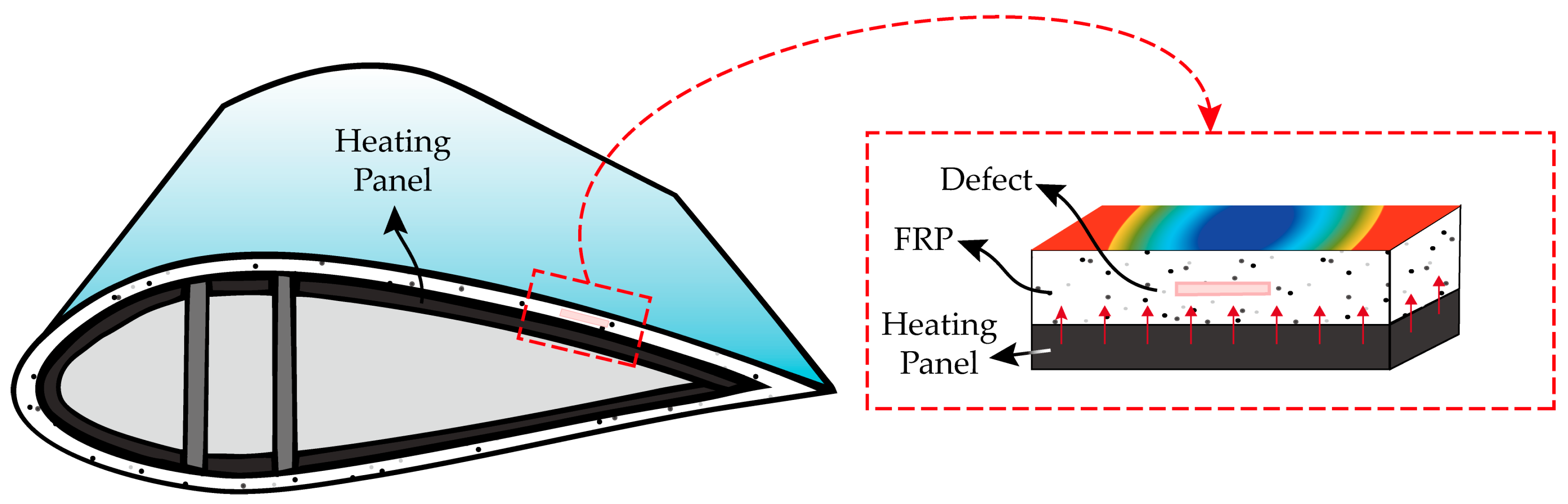
To evaluate the defect detection performance of the deep learning model through experimental methods, 24 real specimens with varying depths and sizes of defects, as well as 6 non-defect real specimens, were fabricated to acquire a real thermographic dataset. The specimens were composed of composite materials with a layered structure of CFRP and GFRP, simulating the cross-section of a wind turbine blade.

CFRP was manufactured using the pultrusion method, with a longitudinal modulus of 145$\mathrm{GPa}$. Each GFRP layer has a thickness of 0.91 mm and is stacked in a [0°/90°] orientation. The epoxy matrix used was KFR-1258L/KFH-164. The entire specimen was fabricated using the resin infusion process.

Table 2. Specification of Real Specimens: ID, Thickness of CFRP and GFRP, and Defect Depth and Size.

Specimen ID	CFRP Thickness	GFRP Thickness	Defect Depth
RN-1, RN-2, RN-3	2.4 mm	6.3 mm	-
RN-4, RN-5, RN-6	2.9 mm	3.6 mm	-
RD29-10,20,30,35,40,50	2.9 mm	3.6 mm	2.9 mm
RD42-10,20,30,35,40,50	2.4 mm	6.3 mm	4.2 mm
RD60-10,20,30,35,40,50	2.4 mm	6.3 mm	6.0 mm
RD78-10,20,30,35,40,50	2.4 mm	6.3 mm	7.8 mm

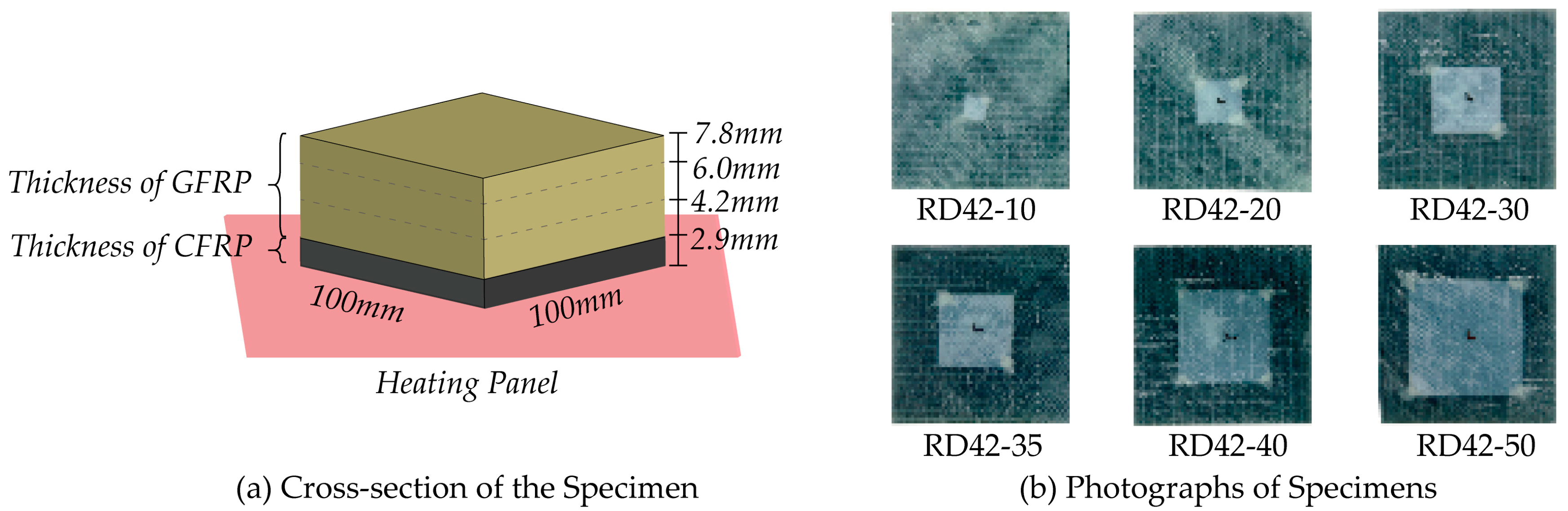
and Figure 2 display the ID of the real specimens, the thickness of CFRP and GFRP, and the depth and size of the defects. Specimens with an ID starting with RN indicate non-defect specimens, while those starting with RD indicate specimens with defects. The number following RD represents the depth (in tenths of a millimeter, 0.1 mm) of the inserted defect, and the last two digits indicate the size of the defect ($\mathrm{width} {\times \mathrm{height} \mathrm{in} \mathrm{mm}}^2$). The thickness of CFRP and GFRP are shown in Figure 2a, and the defects were simulated using Teflon tape with a thickness of 1 mm. The depth of the defect is measured from the heating panel. The defects are square-shaped and consist of five sizes: ${(10 \times 10) \mathrm{mm}}^2,$ ${(20 \times 20) \mathrm{mm}}^2,$ ${(30 \times 30) \mathrm{mm}}^2,$ ${(35 \times 35) \mathrm{mm}}^2,$ ${(40 \times 40) \mathrm{mm}}^2,$ and ${(50 \times 50) \mathrm{mm}}^2$. Figure 2b shows photographs of specimens from RD42-10 to RD42-50, with the white areas representing the defects inserted inside.

The real thermographic data were captured using the FLIR E96 infrared camera on the unheated side with a resolution of $640\times 480$. The defect specimens in the real thermographic dataset were placed on a heating panel, maintaining a uniform temperature of 40 °C and heated using a steady-state thermography method until thermal equilibrium was reached. Due to the limited number of non-defect specimens compared to the defect specimens, these were captured under varying temperature conditions (30 °C, 40 °C) until thermal equilibrium was achieved. Among the non-defect specimens, RN-1 and RN-4 were filmed until the heating panel reached 50 °C from room temperature 22 °C. The thermographic data of RN-1 and RN-4 were used as non-defect class data for training the deep learning model.

The average time required for the heating panel and real specimens to reach thermal equilibrium was 300 s. The acquired thermographic data were cropped to focus on the specimen area and resized to a resolution of $200\times 200$, forming the real thermographic dataset, that is, the real image sequences. Analysis revealed a subtle temperature difference of 0.1 °C to 0.3 °C between the defect and non-defect regions. When using this data as input for the deep learning model, a preprocessing method was necessary to enhance visual contrast by emphasizing the pixel values corresponding to the temperature differences.

Figure 3 illustrates the preprocessing method for the thermographic data from the real specimens. At time $t$, the region $T^t$ of the thermographic data captured by the infrared camera, which corresponds to the specimen, is a square matrix composed of temperature values. Among the $k$ thermographic data consecutively acquired over a certain period, the highest temperature, $T_{\max }^{t:t+k-1}$, and the lowest temperature, $T_{\min }^{t:t+k-1}$, can be defined. The temperature range between $T_{\max }^{t:t+k-1}$ and $T_{\min }^{t:t+k-1}$ is normalized by setting $T_{\max }^{t:t+k-1}$ to 255 and $T_{\min }^{t:t+k-1}$ to 0. Through this process, the square matrices from $T^t$ to $T^{t+k-1}$ are transformed into images.

The minimum temperature observed in a sequence of $k$ consecutive thermographic data is generally represented by $T_{min}^t$ at time $t$, while the maximum temperature is typically represented by $T_{max}^{t+k-1}$ at time $t+k-1$. Through this process, an image that visually maximizes the temperature difference between the defect and non-defect regions in the thermographic data $T^t$ acquired at time $t$ can be obtained.

Setting $t$ to 1 introduces significant noise in a single thermographic image, necessitating the determination of an optimal $t$ value. In this study, $t$ was set to 9 to minimize noise and produce an image that effectively maximizes the contrast between the defect and non-defect regions.

The preprocessing method was applied to the real thermographic dataset obtained from the actual specimens, and the processed thermographic images were assigned to the real thermographic image dataset. This generated dataset was then utilized for performance evaluation as validation data for defect detection in the deep learning model.

Table 3. Class-Wise Distribution of Real Thermographic Image Dataset.

Class	Number of Images	Number of Thermographic Image Sequence
Non-Defect	6638	22
Defect	7755	24

presents the number of data samples in each class that constitute the real thermographic image dataset. Among these, approximately 9% (600 images) of the non-defect class, consisting of two image sequences, were used as the training dataset for the non-defect class of the deep learning model, while approximately 91% (6038 images) were employed for performance evaluation. All 7755 thermographic images from the defect class were used exclusively for performance evaluation.

3.2. Synthetic Thermographic Image Dataset Generation

The synthetic thermographic data were generated using temperature data obtained from the composite material heat transfer analysis, performed with the FEM in the transient thermal analysis module in Ansys 2021 R2.

The purpose of generating synthetic thermographic data, substituting for real thermographic data, was to replicate the temperature variations due to differing heat transfer rates between the defect and non-defect regions in the actual specimens.

The creation of the 3D models for analysis required the fabrication of 26 synthetic specimens, each matching the CFRP thickness, GFRP thickness, defect location, thickness, and size of the 26 real defect specimens. These models were referred to as synthetic specimens. Figure 4 presents the synthetic specimen (SD78-35) corresponding to the real specimen (RD78-35). The synthetic specimens were labeled by modifying the corresponding real specimen IDs, in which ’RD’ was systematically replaced with ’SD’ to maintain consistency in identification. The material properties of the designed synthetic specimens were set as shown in

Table 4. Properties of the Materials.

Material	Density $\left(\mathbf{k}\mathbf{g}/{\mathbf{m}}^3\right)$	$\mathbf{Thermal} \mathbf{Conductivity} \left(\mathbf{W}/\mathbf{m}℃\right)$	$\mathbf{Specific} \mathbf{Heat} \left(\mathbf{J}/\mathbf{k}\mathbf{g}℃\right)$
CFRP [22]	1540	Thermal Conductivityxx = 9.00	1040
		Thermal Conductivityyy = 0.77
		Thermal Conductivityzz = 0.70
GFRP [23]	1600	Thermal Conductivityxx = 0.55	1310
		Thermal Conductivityyy = 0.55
		Thermal Conductivityzz = 0.51
Air	1.225	0.025	1005

. Furthermore, to simulate delamination, defects represented by Teflon tape in the real specimens were modeled as air gaps in the synthetic specimens.

The mesh for analyzing the modeled synthetic specimens was constructed using a hex-dominant method, incorporating a combination of Quad and Tri elements, with an element size of 1 mm. The boundary conditions for the analysis, illustrated in Figure 4c, included setting the temperature of the lower heating element to 40 °C and applying a film convection coefficient of 0.004 W/m² °C to the side and top surfaces, as shown in Figure 4d. The coefficient was initially set to simulate natural convection, gradually increasing to 1 W/m² °C over time. For the interior of the defect, heat transfer was assumed to occur through a stagnant air environment and a very thin film, with a film convection coefficient of 0.004 W/m² °C applied under these conditions. The ambient temperature was set to 22 °C. The analysis was conducted using a time step of 0.1 s over a total duration of 360 s, with the temperature data from the top surface elements of the synthetic specimen recorded and output in matrix form.

3.3. Transformation Process for Aligning Real and Synthetic Thermographic Image Datasets

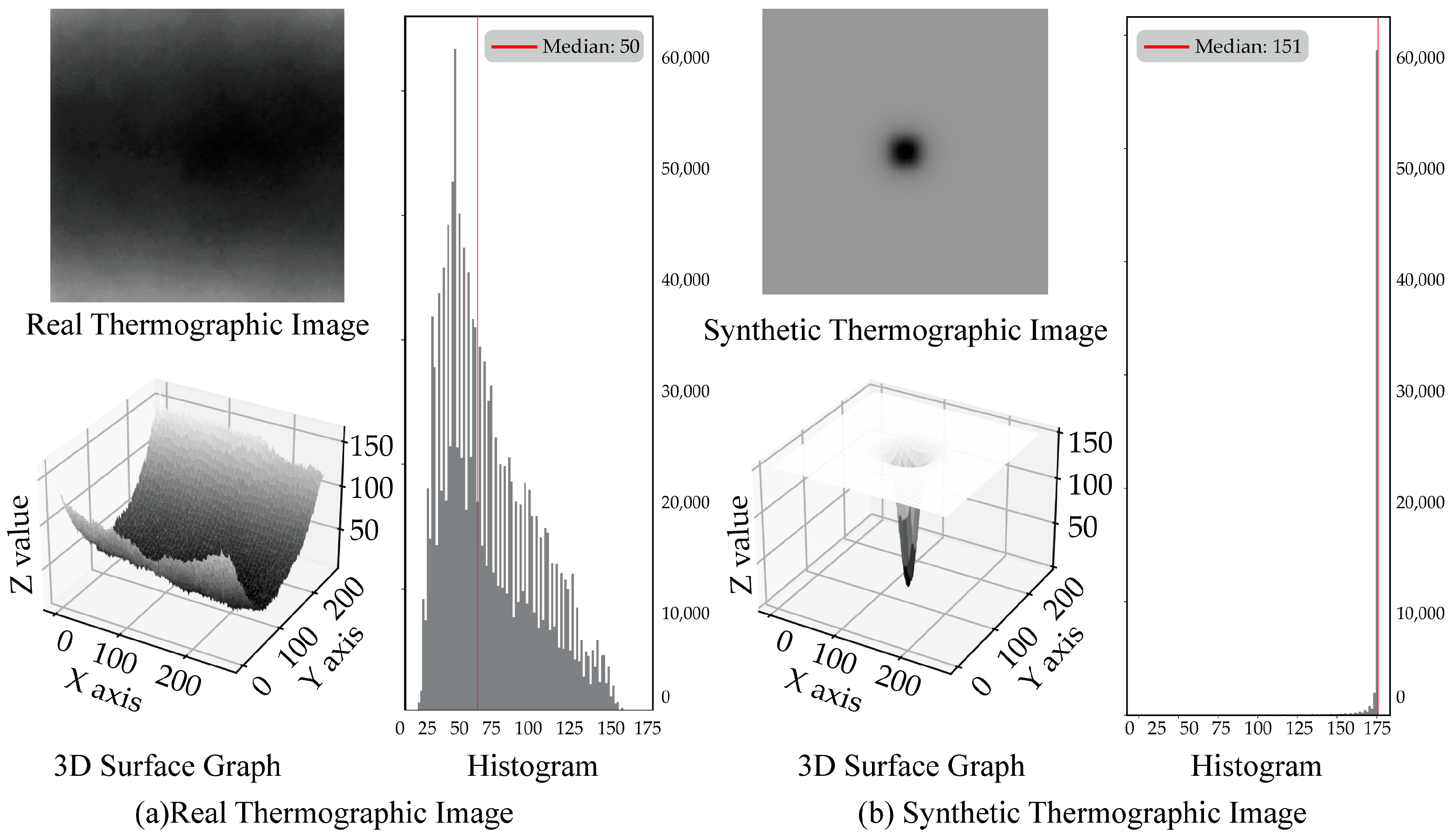
The real thermographic image generated from the actual specimen RD60-35 and the corresponding synthetic thermographic image generated from the synthetic specimen SD60-35 were analyzed for similarity at the same time point (100 s) using a 3D surface graph and histogram. The 3D surface graph represents the elements of a two-dimensional real matrix as depth values, plotted along the x, y, and z axes. The thermographic image of the real specimen at time $t$ is denoted as $RI$, while the thermographic image of the synthetic specimen, generated by normalizing its temperature data, is denoted as $SI$. Both $RI$ and $SI$ are represented as grayscale images with a single channel. Since each pixel in a grayscale image is assigned a scalar $z$ value, it can be represented using a 3D surface graph. The histogram visually illustrates the distribution of the $z$ values from the 3D surface graph [24].

Figure 5a shows the thermographic image $RI$ of the real specimen, obtained at $t=100$, with normalization applied. The pixel values of $RI$ are treated as the depth in the z-direction and reconstructed into a 3D surface graph, along with a histogram representing the distribution of the $z$ values. The curved temperature distribution observed in the 3D surface graph of RI can be attributed to the curvature inherent in the real blade. Since the specimen was fabricated by cutting a portion of the CFRP used in manufacturing the real blade, the blade’s curvature remains. This residual curvature led to heat loss in areas that were not in direct contact during the heating process. Figure 5b presents the thermographic image $SI$ of the synthetic specimen, generated by normalizing the temperature into a 3D surface graph, with a histogram displaying the distribution of the $z$ values.

The median of the $z$ values for $RI$ is 50, with an average of 58, while the median of the $z$ values for $SI$ is 151, with an average of 148. By comparing the 3D surface graph and histogram, the analysis of the images obtained from the real specimen RD60-35 and the corresponding synthetic specimen SD60-35 reveals that the $z$ value distributions of the real thermographic image $RI$ in Figure 5a and the synthetic thermographic image $SI$ in Figure 5b differ significantly. The difference in the $z$ value distributions between the real thermographic image and the synthetic thermographic image, both processed using the same normalization method, can be attributed to the disparity between real and simulated data. Therefore, additional preprocessing is necessary for the synthetic specimen thermographic image $SI$ to minimize this disparity and better align it with the real specimen thermographic image $RI$.

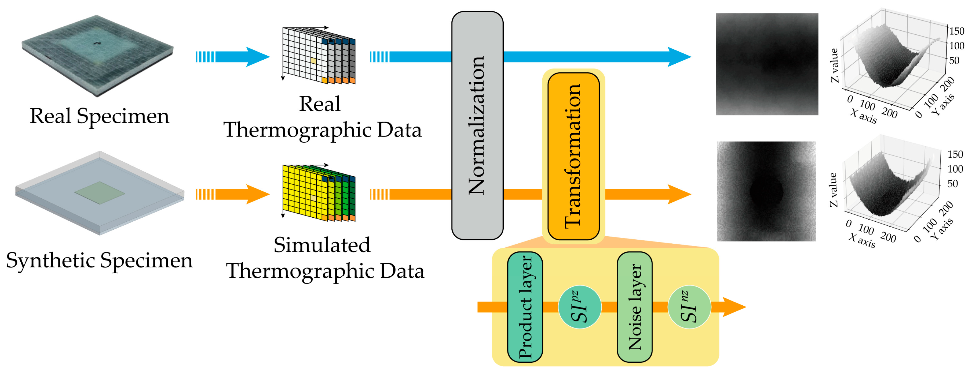
The preprocessing procedure for the synthetic specimen thermographic image $SI$ is shown in Figure 6. The synthetic specimen temperature data passes through the same normalization module applied to the real specimen thermographic data, resulting in the synthetic specimen thermographic image $SI$. Unlike the real specimen thermographic image $RI$, the synthetic specimen thermographic image $SI$ is further processed through a transformation module, where it undergoes the product layer and noise layer stages.

The synthetic specimen thermographic image input into the product layer of the transformation module is a grayscale image, represented by the $z$ value $z_{i,j}$ corresponding to the pixel location $S{I}_{i,j}$, as shown in Equation (1). The $SI$ input into the transformation module is reconstructed into a symmetric surface shape, retaining only the $z$ values $z_{i,j}$ greater than the mean $z.$ This reconstruction occurs within the range from the $\overline{z}$ to the $z_{max}$, symmetrically along the y-axis, with respect to the center of the data. $H$ is the height of the image and $W$ is the width of the image.

$$SI=\left[\begin{array}{cc}\begin{array}{cc}S{I}_{1,1}& S{I}_{1,2}\\ S{I}_{2,1}& S{I}_{2,2}\end{array}& \begin{array}{cc}\cdots & S{I}_{1,W}\\ \cdots & S{I}_{2,W}\end{array}\\ \begin{array}{cc}⋮& ⋮\\ S{I}_{H,1}& S{I}_{H,2}\end{array}& \begin{array}{cc}\ddots & ⋮\\ \cdots & S{I}_{H,W}\end{array}\end{array}\right]=\left[\begin{array}{cc}\begin{array}{cc}{z}_{1,1}& z_{1,2}\\ z_{2,1}& z_{2,2}\end{array}& \begin{array}{cc}\cdots & z_{1,W}\\ \cdots & z_{2,W}\end{array}\\ \begin{array}{cc}⋮& ⋮\\ z_{H,1}& z_{H,2}\end{array}& \begin{array}{cc}\ddots & ⋮\\ \cdots & z_{H,W}\end{array}\end{array}\right]$$

(1)

The reason for reconstructing only those $z_{i,j}$ greater than the $\overline{z}$ is to preserve the characteristics of the $z$ values corresponding to low-temperature data in the regions where $z_{i,j}$ is smaller than the $\overline{z}$, given that $SI$ has a standard deviation close to zero. The output $p{z}_{i,j}$ generated by inputting $z_{i,j}$ into the multiplication layer is expressed as shown in Equation (2).

$$p{z}_{i,j}=\left\{ \begin{array}{c}{\displaystyle \frac{1}{{\left(H/2\right)}^2}}\times {\left(j-\left(H/2\right)\right)}^2, if z_{i,j}>\overline{z}\\ \\ z_{i,j } , if z_{i,j} \le \overline{z}\end{array}\right.$$

(2)

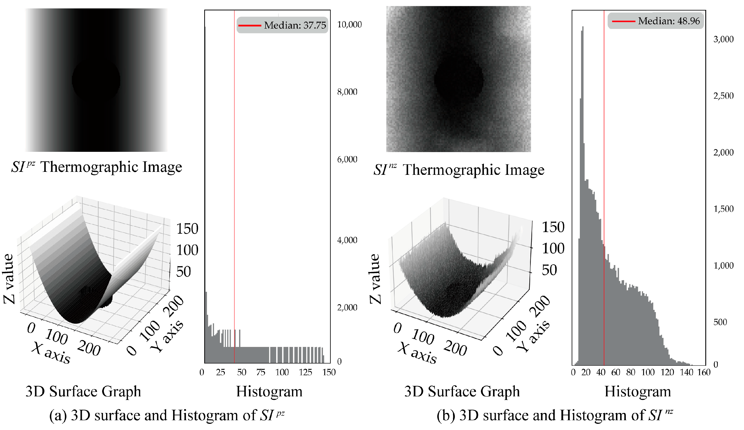
The synthetic specimen thermographic image $SI$ is reconstructed into the $S{I}^{pz}$ matrix, consisting of the $pz$ values output from the computational process in the product layer, resulting in a surface shape similar to $RI$, as shown in the 3D surface graph in Figure 7a. In Figure 7a the maximum and minimum $z$ values in the $S{I}^{pz}$ histogram remain unchanged from the maximum and minimum values of $SI$, but the mean is 49 and the median is 37. This indicates that the data has become more dispersed around the mean, leading to an increase in variance.

However, even though the distribution of $pz$ values in $S{I}^{pz}$ was reconstructed into a surface shape similar to $RI$, it displays a smooth distribution that does not capture the nonlinear characteristics caused by the noise in the real specimen thermographic data of $RI$. Therefore, $S{I}^{pz}$ was input into the noise layer to modify the data distribution.

Figure 7b shows the 3D surface graph and histogram of $S{I}^{nz}$, obtained by inputting $S{I}^{pz}$ into the noise layer. Style transfer is a technique that modifies the style of one image to match that of another, commonly used to apply the style of artworks to photographs or to alter textures [25]. In the noise layer, the style transfer matrix $STM$, generated through style transfer, and a random variable matrix $RM$ with values ranging from 0.9 to 1.1, are used to introduce nonlinear characteristics to the input $S{I}^{pz}$.

One of the non-defect thermographic images from the real specimen dataset was used as the style image for the style transfer model, while the synthetic specimen thermographic image $SI$, prior to its reconstruction into $pz$ values, served as the target image. The style transfer matrix $STM$, as expressed in Equation (3), was constructed accordingly.

$$STM=\left[\begin{array}{cc}\begin{array}{cc}ST{M}_{1,1}& ST{M}_{1,2}\\ ST{M}_{2,1}& ST{M}_{2,1}\end{array}& \begin{array}{cc}\cdots & ST{M}_{1,W}\\ \cdots & ST{M}_{2,W}\end{array}\\ \begin{array}{cc}⋮& ⋮\\ ST{M}_{H,1}& ST{M}_{H,2}\end{array}& \begin{array}{cc}\ddots & ⋮\\ \cdots & ST{M}_{H,W}\end{array}\end{array}\right]$$

(3)

The random variable matrix $RM$ is a matrix composed of values randomly selected from a uniform distribution between 0.9 and 1.1. The random variable matrix $RM$ is expressed as shown in Equation (4).

$$RM=\left[\begin{array}{cc}\begin{array}{cc}R{M}_{1,1}& R{M}_{1,2}\\ R{M}_{2,1}& R{M}_{2,1}\end{array}& \begin{array}{cc}\cdots & R{M}_{1,W}\\ \cdots & R{M}_{2,W}\end{array}\\ \begin{array}{cc}⋮& ⋮\\ R{M}_{H,1}& R{M}_{H,2}\end{array}& \begin{array}{cc}\ddots & ⋮\\ \cdots & R{M}_{H,W}\end{array}\end{array}\right]$$

(4)

In the noise layer, the reconstructed $S{I}^{pz}$ is combined with the style transfer matrix $STM$ and the random variable matrix $RM$, which uses the Hadamard product operation, as shown in Equation (5).

$$n{z}_{i,j}=R{M}_{i,j}\left(0.5\times p{z}_{i,j}+0.5\times ST{M}_{i,j}\right)$$

(5)

$S{I}^{pz}$ is reconstructed into the $S{I}^{nz}$ matrix, consisting of the $nz$ values obtained through the computational process in the noise layer. As shown in Figure 7b, the 3D surface graph and histogram of the reconstructed $S{I}^{nz}$ distribution confirm that it has been transformed to exhibit a distribution similar to that of the real specimen thermographic image $RI$.

The entire synthetic specimen temperature data were fed into the transformation module, and the resulting $S{I}^{nz}$ matrix was converted into an image and assigned to the synthetic thermographic image dataset, which was then used as training data for the deep learning model. For the RD29 specimen, images showing the synthetic thermographic images before and after preprocessing, which vary according to the defect size, are attached in Appendix A.

Table 5. Class-Wise Data Distribution of the Synthetic Thermographic Image Dataset.

Class	Number of Images	Number of Thermographic Image Sequence
Defect	8640	24

shows the distribution of data by class in the synthetic thermographic image dataset. The non-defect class is composed of 14% of the non-defect class data from the real thermographic image dataset.

3.4. Analysis of Similarities Between Real and Synthetic Thermographic Image Datasets

The similarity of the synthetic thermographic image dataset, constructed for training the deep learning model, was analyzed in comparison to the real thermographic image dataset. Before inputting the synthetic thermographic image dataset obtained from the synthetic specimen into the transformation module, the variation in specific pixel values at certain coordinates in consecutive thermographic images was expressed as a normal distribution. After inputting the synthetic thermographic image dataset into the transformation module, the variation in specific pixel values at the same coordinates in consecutive thermographic images was again expressed as a normal distribution. This was then compared to the normal distribution representing the variation in specific pixel values at the corresponding coordinates in the real thermographic image dataset of the real specimen. The analysis evaluated the effectiveness of preprocessing via the transformation module in enhancing the similarity between the synthetic and real thermographic image datasets.

The difference in pixel values at specific coordinates between the synthetic thermographic images at time $t$ and $t+1$ in the synthetic thermographic image dataset was defined as the pixel value rate of change. This definition was designed to effectively simulate the contrast in the temperature rate of change resulting from the difference in heat transfer rates between the defect and non-defect regions observed in the real specimen. The similarity between the pixel value rate of change in the synthetic thermographic dataset and the rate of change distribution in the real thermographic image dataset indicates that the temperature data obtained from the synthetic specimen faithfully reproduces the physical characteristics of the real data.

Figure 8 presents the pixel value rates of change, ranging from 0 to 255, over time at 15 randomly selected coordinates in the defect region and 15 randomly selected coordinates in the non-defect region, from both the real thermographic image dataset obtained from the RD60-30 specimen and the synthetic thermographic image dataset obtained from the SD60-30 specimen. The pixel value rates of change are expressed as a normal distribution. By comparing the rate of change in pixel values over time of the real thermographic image dataset and the pre-transformation and post-transformation synthetic thermographic image datasets using the normal distributions shown in Figure 8, the effectiveness of the transformation module, aimed at making the synthetic thermographic image dataset resemble the real thermographic image dataset, was evaluated.

In Figure 8, the blue line represents RID, indicating the distribution of the rate of change in pixel values at specific coordinates extracted from the real thermographic image dataset. The gray line represents SID (pre-transformation), showing the distribution of the rate of change in pixel values extracted from the synthetic thermographic image dataset before being input into the transformation module. The yellow line represents SID (post-transformation), showing the distribution of the rate of change in pixel values extracted from the synthetic thermographic image dataset after processing by the transformation module. The x-axis (rate of change) of the graph displays the rate of change in pixel values at selected coordinates over time. The y-axis represents the probability density, indicating the likelihood of the occurring specific pixel value change rates (x-axis value).

The mean pixel value change rate distribution RID in the real thermographic image dataset is 0.139. In comparison, the mean pixel value change rate distribution SID of Pre-Transformation in the synthetic thermographic image dataset is 0.347, while the mean SID of Post-Transformation is 0.086. After transformation, the mean of the synthetic thermographic image dataset moves approximately 0.155 (74%) closer to the mean of the real thermographic image dataset compared to the pre-transformation dataset. Thus, the transformation module improves the similarity between the synthetic and real thermographic image datasets in terms of their means. This demonstrates that the transformation module effectively adjusts the central tendency of the synthetic thermographic image dataset to align more closely with that of the real thermographic image dataset.

The standard deviation of the pixel value change rate distribution RID in the real thermographic image dataset is 4.193. In comparison, the standard deviation of the pixel value change rate distribution SID (Pre-Transformation) in the synthetic thermographic image dataset before transformation is 0.902, while the standard deviation of SID (Post-Transformation) after transformation is 2.201. Following the transformation, the standard deviation of the synthetic thermographic image dataset becomes approximately 1.299 (39.5%) closer to that of the real thermographic image dataset compared to the pre-transformation dataset. This indicates that the transformation module improves the similarity between the synthetic and real thermographic image datasets in terms of standard deviation.

Since the standard deviation represents the spread of the data distribution, it can be concluded that the transformation module adjusts the distribution of the synthetic dataset to better match that of the real thermographic dataset. Across all specimen IDs, the transformation module proves to be an effective method for narrowing the gap between the synthetic and real thermographic datasets, particularly by improving their similarity in terms of the mean and the standard deviation.

4. Performance Evaluation and Analysis

4.1. Deep Learning Model Selection

In this study, ResNet-50 [26], DenseNet-121 [27], and Vision Transformer (ViT) [28] models were employed to evaluate the defect detection performance of deep learning models trained on synthetic thermographic datasets when applied to real thermographic datasets. Leveraging the architectural strengths of each model, ResNet-50, DenseNet-121, and ViT were used as key application models to compare the defect detection performance on real thermographic data when trained with synthetic thermographic data.

ResNet-50 is an architecture that effectively addresses the gradient vanishing problem, a common challenge in deep learning models, through the introduction of residual connections. A residual connection directly adds the input to the output of the subsequent layer, preserving the original input signal while enabling the model to learn transformed information simultaneously. This design ensures stable training even in deep network architectures, alleviates the gradient vanishing problem, and facilitates effective interaction between low-level and high-level information [26].

DenseNet-121 is an architecture designed to maximize the sharing of feature information across layers by introducing a dense connection structure, where the output of each layer is connected to all subsequent layers. With dense connections, each layer receives the outputs of all preceding layers as input, reducing information loss and enabling the effective learning of complex features with fewer parameters. These structural characteristics promote efficient gradient flow, ensuring stability during training even in very deep networks [27].

The Vision Transformer (ViT), unlike Convolutional Neural Network (CNN)-based architectures such as ResNet-50 and DenseNet-121, processes images by dividing them into patches and treating them as sequence data, excelling in learning global relationships. This capability makes ViT particularly effective for defect detection in composite materials with complex structures, as it enables the understanding of global patterns and the identification of relationships between defect regions [28].

The optimizer for each deep learning model was the Adam optimizer, with the learning rate set to 0.001 [29]. The batch size was configured as 64, and training was conducted for up to 100 epochs. However, early stopping was applied to all three models at the 10th epoch, as no further improvements in loss were observed. Binary Cross-Entropy Loss was utilized for binary classification in defect detection.

This study employed transfer learning to enhance the training efficiency of ResNet-50, DenseNet-121, and ViT. Pretrained weights from ImageNet were used to initialize all three models. Fine-tuning was performed on all layers, allowing the models to effectively adapt to the features of the synthetic thermographic data.

4.2. Evaluation Metrics

In this study, accuracy, precision, recall, Negative Predictive Value (NPV), and specificity were utilized as evaluation metrics to quantitatively assess the defect detection performance of the deep learning models. Accuracy serves as a fundamental measure for evaluating the overall classification performance of the models. Precision represents the proportion of predictions identified as defective that are indeed defective, assessing the reliability of the model’s defect predictions. NPV indicates the proportion of predictions classified as non-defective that are truly non-defective, measuring the reliability of the model’s non-defect predictions. Recall represents the proportion of actual defective thermographic images correctly identified as defective by the model, evaluating how well the model detects defective images without missing any. Specificity represents the proportion of actual non-defective thermographic images correctly classified as non-defective, assessing how well the model detects non-defective data without overlooking any.

In this study, these evaluation metrics were comprehensively applied to compare and analyze the defect detection performance of ResNet-50, DenseNet-121, and ViT models trained on synthetic thermographic datasets. Pre-ResNet-50, Pre-DenseNet-121, and Pre-ViT refer to models trained on unprocessed synthetic thermographic datasets, while Post-ResNet-50, Post-DenseNet-121, and Post-ViT refer to models trained on preprocessed synthetic thermographic datasets. Each model was evaluated based on accuracy, precision, recall, NPV, and specificity to identify the most suitable deep learning architecture for defect detection. Additionally, the impact of preprocessing on defect detection performance was analyzed. This approach validated the feasibility and effectiveness of the proposed synthetic data-based methodology.

4.3. Results and Discussion

4.3.1. Impact of Preprocessing on Model Performance

Table 6. Performance Metrics of Deep Learning Models Before and After Applying the Transformation Module on Synthetic Thermographic Image Datasets.

Model	Accuracy	Precision	Recall	NPV	Specificity
RID-ResNet-50	52.54%	30.06%	99.55%	99.71%	40.46%
RID-DenseNet-121	39.64%	25.28%	99.81%	99.79%	24.18%
RID-ViT	56.68%	32.06%	99.94%	99.96%	45.56%
Pre-ResNet-50	34.30%	7.92%	1.59%	37.64%	76.32%
Pre-DenseNet-121	37.38%	21.55%	4.31%	39.38%	79.86%
Pre-ViT	44.32%	57.34%	3.38%	43.82%	96.34%
Post-ResNet-50	37.84%	13.79%	2.01%	39.98%	83.85%
Post-DenseNet-121	35.67%	31.26%	12.02%	36.89%	66.06%
Post-ViT	51.62%	94.57%	14.81%	47.48%	98.91%

presents the defect detection performance of the selected deep learning models on the real thermographic image dataset when trained with the synthetic thermographic image dataset before and after preprocessing. Through Table 6, the impact of applying the transformation module to the synthetic thermographic image dataset on performance can be analyzed.

Improvements in accuracy, NPV, and specificity were observed with ResNet-50 and ViT, whereas DenseNet-121 showed a decline in performance. The observed improvements with ResNet-50 and ViT were analyzed by examining changes in the feature maps generated at their respective layers. The real thermographic images in Figure 9a, Figure 10a, and Figure 11a represent cases where the Pre-models failed to classify correctly, but the Post-models successfully classified them. Figure 9 illustrates the feature maps produced by Pre-ResNet-50 and Post-ResNet-50 for the same real thermographic image, while Figure 10 presents those generated by Pre-ViT and Post-ViT. These differences in the feature maps suggest that the models effectively reduced the domain gap between real and synthetic data through the transformation module, thereby enhancing data similarity.

In contrast, DenseNet-121 appears to have struggled in learning the characteristics of the transformed data produced by the transformation module. The variations in performance metrics are likely due to differences in the classifier layer. Figure 11 shows the feature maps generated by Pre-DenseNet-121 and Post-DenseNet-121 for the same real thermographic image, which appear almost identical. A comparison of the weights and biases in the classifier layers revealed that the weight differences ranged from −0.04 to 0.03, and the bias differences were 0.04 and 0.03, respectively. These findings indicate that, despite similar feature maps, the two models established distinct decision boundaries.

These differences were further validated using cosine similarity and Euclidean distance metrics. The cosine similarity between the weight vectors of the two models was 0.458, indicating significantly different weight directions, while the Euclidean distance was 1.16, reflecting a notable disparity in weight magnitudes. Consequently, these differences in weights and biases were identified as the primary reasons for the divergent classification outcomes despite identical feature maps.

The impact of these weight and bias differences on performance metrics shows that Post-DenseNet-121 achieved improved recall and precision compared to Pre-DenseNet-121. This suggests greater reliability in predicting the positive class. However, this improvement came at the expense of reduced accuracy and specificity, as predictions for the negative class became less reliable.

In the context of defect detection in wind turbine blades, it is crucial to predict defects accurately without missing them. The performance metrics associated with this requirement are precision and recall. The application of the transformation module to the synthetic thermographic image dataset impacted the performance of all models, demonstrating significant improvements, particularly in precision and recall for defect detection. Precision, which represents the probability that a prediction of a defect corresponds to an actual defect, improved by 5.87% in ResNet-50, 9.71% in DenseNet-121, and 37.23% in ViT. Recall, which indicates the proportion of actual defective data correctly identified by the model, improved by 0.42% in ResNet-50, 7.71% in DenseNet-121, and 11.43% in ViT. These results suggest that the transformation module enhances the physical characteristics of defect regions to more closely resemble those in real thermographic image data, thereby improving the reliability of deep learning models for defect detection.

4.3.2. Model-Specific Performance Insights

The performance comparison of Post-ResNet-50, Post-DenseNet-121, and Post-ViT, trained using the synthetic thermographic image dataset with the transformation module applied, revealed that Post-ViT demonstrated the best performance. Post-ViT achieved an accuracy of 51.62%, approximately 14% higher than the other models. It recorded a specificity of 98.91%, indicating its ability to detect nearly all non-defective data without omission. Precision was 94.57%, reflecting a high probability that predictions of defects correspond to actual defects. Furthermore, Post-ViT achieved the highest recall value of 14.81%, outperforming the other models. These results highlight the overall superiority of ViT in defect detection performance.

Conventional CNN-based models such as ResNet-50 and DenseNet-121 primarily focus on local features, making it challenging to capture spatially distant relationships between temperature variations. The superior performance of ViT compared to ResNet-50 and DenseNet-121 can be attributed to its ability to effectively learn the interactions between spatially distributed temperatures in thermographic data. In the thermographic data from wind turbine blades, heat transfer characteristics caused by defects often exhibit complexity, where the temperature at a specific location can influence distant, non-adjacent areas. ViT excels in capturing such global relationships.

The self-attention mechanism in ViT effectively models the interactions between spatially distant temperature changes, enabling it to reflect the complex heat transfer characteristics of wind turbine blades. This is evidenced by its high performance in specificity, precision, and recall, positioning ViT as the most effective model for defect detection among the evaluated architectures.

The performance of deep learning models trained on the real thermographic image dataset was experimentally compared with that of models trained exclusively on the synthetic thermographic image dataset. RID-ResNet-50, RID-DenseNet-121, and RID-ViT are deep learning models trained using 80% of the real thermographic image dataset as the training set, with the remaining 20% of the data, which was not used during training, serving as the evaluation set.

When compared to Post-ResNet-50, Post-DenseNet-121, and Post-ViT, the differences in accuracy were relatively small: 13.7% for ResNet-50, 2.97% for DenseNet-121, and 5.06% for ViT. This can be attributed to the lack of contrast between defective and non-defective areas in the early and late heating stages when the specimen approaches thermal equilibrium, which results in the disappearance of the characteristic features of the defect class. Figure 12a shows the thermographic image of the RD78-50 specimen obtained at a heating time of 4 s, while Figure 12b shows the image obtained at a heating time of 150 s. At 150 s, a clear contrast between defective and non-defective areas is observed. These findings suggest that the physical characteristics of thermal equilibrium observed in thermographic datasets can negatively impact the model’s performance.

4.3.3. Analysis of Model Performance Based on Defect Depth and Size

Table 7. Comparison of Model Accuracy Pre- and Post-Processing Based on Defect Depth.

Defect Depth	Pre-ResNet-50	Post-ResNet-50	Pre-DenseNet-121	Post-DenseNet-121	Pre-ViT	Post-ViT
RN-1~RN-6	76.32%	83.85%	79.86%	66.06%	96.34%	98.91%
2.9 mm (RD29)	1.06%	0.00%	2.27%	4.23%	13.48%	5.81%
4.2 mm (RD42)	1.49%	0.10%	3.33%	13.18%	0.31%	8.26%
6.0 mm (RD60)	3.79%	4.30%	6.06%	18.11%	1.79%	24.55%
7.8 mm (RD78)	0.00%	3.52%	5.46%	12.26%	0.05%	20.33%

presents the accuracy results based on defect depth. An analysis of Table 7 indicates that the models incorporating the transformation module tend to achieve higher accuracy for specimens with defects located farther from the embedded heating panel. For the RD60 real specimen, accuracy improved by 0.51% with the ResNet-50 model, 12.05% with the DenseNet-121 model, and 22.76% with the ViT model. Similarly, for the RD78 real specimen, accuracy increased by 3.52% with the ResNet-50 model, 6.8% with the DenseNet-121 model, and 20.28% with the ViT model.

However, for specimens with defects located closer to the embedded heating panel, a decrease in accuracy was observed. Specifically, the accuracy for the RD20 real specimen decreased by 1.06% with the ResNet-50 model and by 1.49% for the RD42 real specimen. Furthermore, the accuracy for the RD29 real specimen decreased by 7.68% with the ViT model.

When the embedded heating panel is in close proximity to the defect, the thermal signals generated through heat transfer weaken due to the material’s absorption and dissipation of heat. As a result, although the time required for heat to reach the defect is shorter, the thermal signal is attenuated by the material in front of the defect, making the temperature difference between defective and non-defective regions less distinguishable. This likely indicates that the transformation module failed to generate synthetic data capable of adequately capturing these subtle temperature differences, thereby limiting the model’s ability to learn from such variations.

Thus, the model appears to have insufficiently learned the subtle temperature variations present in the RD29 real specimen and instead prioritized learning from stronger thermal signals. Consequently, while accuracy improved for deeper defects in the RD42, RD60, and RD78 real specimens, accuracy declined for the shallower defect in the RD29 real specimen.

Table 8. Comparison of Model Accuracy Pre- and Post-Processing Based on Defect Size.

Defect Size (mm2)	Pre-ResNet-50	Post-ResNet-50	Pre-DenseNet-121	Post-DenseNet-121	Pre-ViT	Post-ViT
RN-1~RN-6	76.32%	83.85%	79.86%	66.06%	96.34%	98.91%
$10\times 10$	0.79%	2.59%	8.72%	16.18%	8.33%	12.18%
$20\times 20$	0.92%	0.00%	4.98%	13.78%	11.03%	30.25%
$30\times 30$	0.62%	0.23%	4.11%	11.62%	3.56%	23.70%
$35\times 35$	3.46%	6.00%	1.84%	8.46%	0.00%	0.00%
$40\times 40$	3.45%	3.14%	4.29%	10.73%	0.00%	6.82%
$50\times 50$	0.23%	0.00%	1.88%	11.34%	0.08%	15.95%

presents the accuracy results based on defect size. An analysis of Table 8 reveals that, with a few exceptions in the ResNet-50 model, accuracy generally improves as defect size increases. Smaller defects often exhibit minimal temperature differences, making them more challenging for the models to detect. However, the transformation module effectively amplified these temperature differences, leading to enhanced detection performance in the DenseNet-121 and ViT models.

The Pre-models generally demonstrated higher performance compared to the Post-models. Thus, it can be inferred that the transformation module effectively improves model performance by reducing the domain gap between synthetic and real data. Furthermore, the Post-ViT model exhibited the most stable and superior performance regardless of defect size and depth. It consistently maintained high accuracy under various defect conditions, indicating that the transformer-based architecture effectively captures complex defect patterns. However, there remains a need to enhance overall defect detection performance. Future research could focus on developing hybrid models or employing ensemble techniques to address the weaknesses in individual models and further improve robustness.

5. Conclusions and Future Directions

This study aimed to address the class imbalance problem that arises in anomaly detection environments when applying deep learning for defect detection in wind turbine blades. To achieve this, synthetic thermographic datasets were generated through heat transfer analysis using the finite element method. To minimize the domain gap between the generated synthetic datasets and the real data, a transformation module was proposed. The performance of deep learning models trained on synthetic thermographic datasets with the proposed transformation module was evaluated through a comparative analysis in experimental settings, both before and after applying the module.

By comparing the performance of models trained using synthetic thermographic datasets without the transformation module to those trained using datasets with the module applied, it was confirmed that the transformation module effectively reduces the gap between synthetic and real data, thereby improving defect detection performance. Notably, it proved effective in enhancing precision and recall for defect detection. This demonstrates that the transformation module contributed to aligning the physical characteristics of synthetic thermographic images more closely with those of real data.

Among the selected models, ViT recorded the highest accuracy (51.62%), specificity (98.91%), and precision (94.57%), showcasing its overall superior performance. This outcome underscores ViT’s capability to effectively capture the global relationships between spatially distributed temperatures in thermographic data through its self-attention mechanism.

However, all models, including ViT, demonstrated limitations in specific performance metrics for defect detection. In particular, recall remained low across all models, highlighting the inability to completely eliminate false positives and false negatives in defect detection. Moreover, despite ViT’s high specificity and precision, its performance was insufficient to meet the requirements for practical application in defect detection.

It was also observed that the physical characteristics of thermal equilibrium present in the thermographic dataset can negatively impact model performance. This issue arises from the temporal properties inherent in thermographic data and should be considered to provide inspectors with reliable defect detection results. Further research is necessary to enhance the overall defect detection performance by taking into account the temporal characteristics of thermographic data.

This study demonstrated that defect detection performance can be enhanced through the utilization of synthetic data and preprocessing techniques, thereby establishing a foundation for the development of more advanced defect detection technologies to ensure the stable operation and maintenance of wind turbine blades. Future research should aim to further enhance overall defect detection performance, with particular attention to improving recall for wind turbine blades.