Research on Active Control of X-Type Interconnected Hydropneumatic Suspensions for Heavy-Duty Special Vehicles via Extended State Observer-Model Predictive Control

Abstract

To address the weak adaptability of the passive X-type interconnection hydropneumatic suspension to different road surfaces and the poor performance of traditional single-control methods, an active controller based on the extended state observer (ESO) and model predictive control (MPC) was designed for the X-type interconnection hydropneumatic suspension of heavy-duty special vehicles. First, the structure of the X-type interconnection hydropneumatic suspension was analyzed. A three-degree-of-freedom (DOF) linearized hydropneumatic suspension model with disturbances was established based of the seven-DOF full-vehicle model of the active X-type interconnection hydropneumatic suspension. The disturbances were analyzed, and a disturbance ESO was developed. A controller for MPC was subsequently designed based on the linearized state space model, forming a controller for ESO-MPC. Simulations were conducted on both C-class random roads and convex pavement, with fuzzy PID control included for comparison. The simulation results demonstrated that, compared with the passive X-type interconnection hydropneumatic suspension, the active suspension with the controller for ESO-MPC achieved reductions in body vertical acceleration, pitch angular acceleration, and roll angular acceleration of 18.7%, 24.7%, and 26.1%, respectively, on Class C random roads. With fuzzy PID control, the reductions were 5.59%, 7.99%, and 15.54%, respectively. For convex pavement, the controller for ESO-MPC reduced body vertical acceleration, pitch angular acceleration, and roll angular acceleration by 36.5%, 21.2%, and 18.1%, respectively, whereas fuzzy PID control resulted in reductions of 14.04%, 10.6%, and 7.92%, respectively. Compared with fuzzy PID control, the controller for ESO-MPC significantly improved the performance of the hydropneumatic suspension system, achieving precise control of the X-type interconnection hydropneumatic suspension system for heavy-duty special vehicles, thereby enhancing ride comfort and stability.

1. Introduction

Hydropneumatic suspensions have superior nonlinear stiffness and damping characteristics, and interconnected hydropneumatic suspensions can achieve different performance requirements through different interconnection forms, such as anti-roll, anti-pitch, and anti-vertical functions. Hydropneumatic suspensions are often used in special vehicles. Compared with those of ordinary heavy vehicles, the road conditions of special vehicles are complex and changeable, and they require greater mobility. Passive X-type interconnected hydropneumatic suspensions can provide both anti-roll and anti-pitch moments, with superior performance, a simple structure, and easy implementation. After being designed and installed, their stiffness and damping can be fixed. When road excitation changes and depending on whether the load is empty or full, the corresponding optimal stiffness and damping are different. The suspension may be too hard or too soft, which limits the performance improvement of special vehicles. In addition, if the hydropneumatic suspension works under a high load for a long time, it may also cause accidents such as leakage, thereby shortening the service life of the suspension and reducing safety. Active suspensions can control the filling and discharging of oil and gas spring cylinders through an external oil source, achieving the active control of interconnected hydropneumatic suspensions. This effectively improves the smoothness and stability of a vehicle under different road excitations or empty as opposed to full loads.

Scholars globally have directed their attention to control methodologies. Shi Yunxu et al. [1] constructed a semi-vehicle dynamic model and devised a fuzzy PID controller to regulate the active hydropneumatic suspension’s output force, leading to notable enhancements in suspension performance. Zhang Jie et al. [2] created a two-DOF (degrees of freedom) active suspension model for a quarter-car setup, formulated fuzzy control rules, and engineered fuzzy controllers accordingly. Nguyena D N et al. [3] examined the influence of SMC (sliding-mode control)-based active suspension on automotive performance. Sathishkumar P. [4] introduced an MPC active suspension system, utilizing body state identification to determine the braking model and thereby manage the suspension damping force. Gokul P S et al. [5] proposed an LQR controller optimized by a particle swarm optimization algorithm, simulating both passive and adaptive dynamic models of air suspension systems. Yang Qiyao and colleagues [6] crafted a fuzzy PID controller tailored to a quarter-vehicle model featuring active air suspension. Caponetto R et al. [7] incorporated fuzzy control into a seven-DOF model of a hydropneumatic suspension. Zhang Jie [8] proposed an active hydraulic interconnected suspension system based on robust $H\infty$ control.

The above single-control method often has difficulty in meeting the performance requirements of heavy-duty special vehicles, and the composite control theory combined with a variety of control strategies can lead to more efficient, accurate, and stable system control. An active controller leveraging both ESO and MPC was devised to overcome the challenges posed by the passive X-type interconnected hydropneumatic suspension’s limited adaptability to diverse road surfaces and the inadequate performance of traditional single-mode control strategies. The improved controller for MPC based on the ESO accurately controls the output force of the hydropneumatic suspension, and the hydropneumatic suspension’s performance is refined, resulting in improved ride comfort and stability for special vehicles.

Compared with fuzzy PID, ESO-MPC can handle multivariable and nonlinear systems, estimate unmodeled dynamics, and external disturbances of the system through an extended state observer (ESO) and has stronger disturbance resistance [9]. MPC can explicitly handle constraints (such as input and state constraints) by optimizing future state trajectories [10]. The stability of the system is relatively high [11], whereas fuzzy PID is typically suitable for single-variable or simple nonlinear systems and cannot directly handle constraints [12]. Compared with sliding-mode control, ESO-MPC optimizes the control input to smooth the control signal and avoid the common chattering problem in sliding-mode control. ESO-MPC can also handle constraints explicitly, whereas sliding-mode control is often difficult to use to directly handle constraints [13]. Compared with LQR, ESO-MPC can handle nonlinear systems and constraints, whereas LQR is only applicable to linear systems. ESO-MPC has stronger robustness when it estimates disturbances and unmodeled dynamics through ESO, whereas LQR is more sensitive to model accuracy and disturbances [14]. In summary, ESO-MPC can explicitly handle system constraints (input and state constraints) and estimate disturbances and unmodeled dynamics through ESO, has strong robustness, and is suitable for nonlinear and multivariable systems [15]. However, the computational complexity is high, and the hardware requirements are high, so the real-time performance may not be as good as control methods such as LQR.

2. Material and Methods

2.1. Dynamic Model of Hydropneumatic Suspension

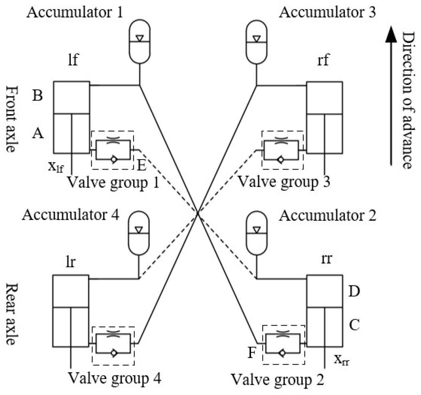
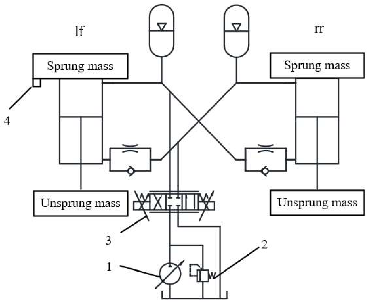
2.1.1. Active X-Type Interconnecting Hydropneumatic Suspension System

As illustrated in Figure 1, the passive X-type interconnected hydropneumatic suspension is linked by connecting the left front and right rear hydropneumatic springs, as well as the right front and left rear hydropneumatic springs. When a special vehicle operates under normal conditions, the interconnected hydropneumatic suspension absorbs the force of the pavement via compressibility and elastic deformation of the gas. When the vehicle brakes, the body leans forward, the front axle’s suspension generates high pressure, and the oil in the upper cavity of the front axle’s hydropneumatic spring flows into the lower cavity of the rear axle’s hydropneumatic spring, resulting in the rear axle’s suspension following compression. The rear axle’s suspension also follows the same law when the vehicle starts, which inhibits the pitching movement of the body. When the vehicle turns right, the body is in a left-leaning state, the left suspension is compressed, and the oil from the upper chamber of the left front hydropneumatic spring migrates into the lower chamber of the right rear hydropneumatic spring, causing the right suspension to follow compression. When turning left, the right side of the body also follows the same law, which inhibits the body’s roll movements. Therefore, X-type interconnected hydropneumatic suspensions can improve the pitch and roll stiffness at the same time. Therefore, the vehicle’s pitch and roll movements are effectively dampened by this process.

Wu Xiaojian et al. added a fuel supply system to the passive oil–gas suspension to form an active interconnected hydropneumatic suspension, which is the most common system [16]. This article adopts the same active X-type interconnected hydropneumatic suspension structure as shown in Figure 2, which shows the active control modules added by the left front and right rear hydropneumatic springs. In contrast with the passive X-type interconnected suspension, the active suspension is equipped with a hydraulic pump, a safety valve, a servo valve, and an angle sensor, where monitoring the car body’s pitch and roll angles in real time provides crucial data for the suspension system. After receiving the information on the car body, the controller controls the servo valve via an electrical signal to fuel or unload the interconnected hydropneumatic suspension, and the system actively controls the output force of the hydropneumatic spring cylinder, adapting to different road excitations and thereby improving suspension performance.

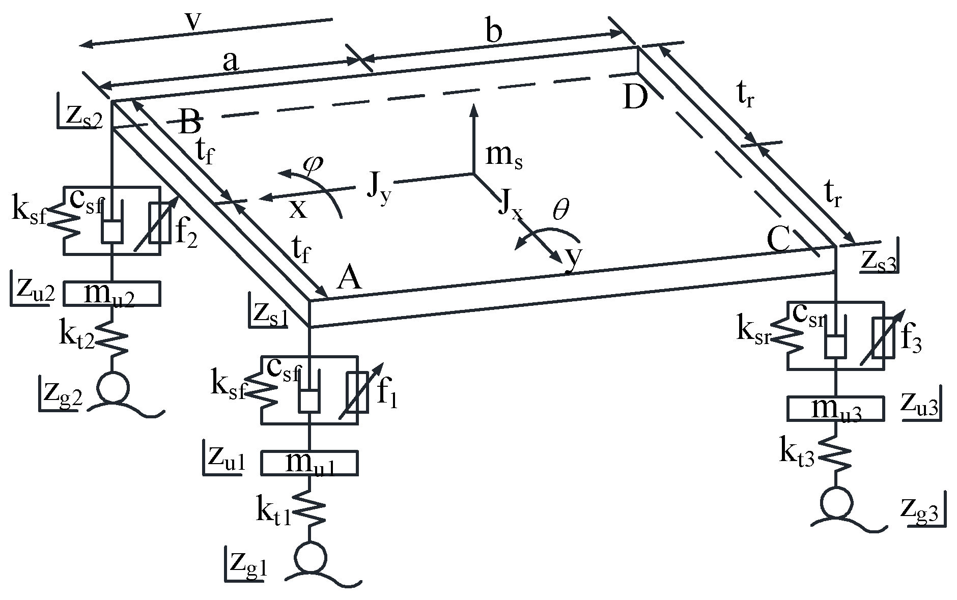
2.1.2. Seven-DOF Model

The seven-DOF vehicle model system is a strongly coupled multiple-input and multiple-output system. Figure 3 illustrates the structural diagram of a vehicle with seven DOFs. The seven DOFs are as follow: vertical displacement $z_s$, roll angle $\theta ,$ pitch angle $\phi$, and $A, B, C, \mathrm{and} D,$ which are the four positions under the spring quality of vertical displacement for $z_{ui}$ ($i=1, 2, 3, 4$). In Figure 3, $m_s$ is the body quality; $J_x$ represents the pitching moment of inertia; $J_y$ represents the roll moment of inertia; $m_{ui}$ ($i=1, 2, 3, 4$) indicates the four unsprung mass locations, denoted as $A, B, C, \mathrm{and} D$; $k_{si}$ ($i=1, 2, 3, 4$) indicates the four locations ($A, B, C, \mathrm{and} D$)’ suspension spring stiffness; $c_{si}$ ($i=1, 2, 3, 4$) corresponds to the four positions ($A, B, C, \mathrm{and} D$)’ suspension shock absorber damping; $k_{ti}$ ($i=1, 2, 3, 4$) is the stiffness of four tires; $z_{gi}$ ($i=1, 2, 3, 4$) represents the displacement of four tires; $f_i$($i=1, 2, 3, 4$) represents the controllable output force; $t_f$ and $t_r$ represent half of the track width for the front and rear suspensions, respectively; and $a$ and $b$ are the distances from the center of mass to front and rear axes, respectively.

When the car body’s vibration is small, $\sin \theta \approx \theta$ and $\sin \phi \approx \phi$. The vertical displacement of bodies A, B, C, and D $z_{si}$ is as follows:

$$\begin{array}{c}{z}_{s1}\approx z_s-a\theta +t_f\phi \\ z_{s2}\approx z_s-a\theta -t_f\phi \\ z_{s3}\approx z_s+b\theta +t_r\phi \\ z_{s4}\approx z_s+b\theta -t_r\phi \end{array}$$

(1)

If we define $Z_m=\left[ z_s \theta \phi \right]$, $Z_s=\left[z_{s2} z_{s2} z_{s3} z_{s4}\right]$. Adopting matrix notation allows for a simplified representation, as follows:

$$Z_s=L^T{Z}_m$$

(2)

where L is the transformation matrix, which can be expressed as

$$L=\left[\begin{array}{cccc}1& 1& 1& 1\\ -a& -a& b& b\\ t_f& -t_f& t_r& -t_r\end{array}\right]$$

(3)

Using Newton’s second law, a differential equation governing the seven-DOF vibrations of the vehicle is formulated. Specifically, the differential equation related to vertical vibrations is as follows:

$$M_s{\ddot{z}}_s-\sum _{i=1}^4(F_{ksi}+F_{csi}+f_i)=0$$

(4)

The differential equation of pitch motion in the vertical plane can be formulated as follows:

$$J_x\ddot{\theta }+a\sum _{i=1,2}(F_{ksi}+F_{csi}+f_i)-b\sum _{i=3,4}(F_{ksi}+F_{csi}+f_i)=0$$

(5)

The differential equation of the car body’s roll motion can be formulated as follows:

$$\begin{array}{l}{J}_y\ddot{\phi }+t_f{\displaystyle \sum _{i=1,2}}{(-1)}^i(F_{ksi}+F_{csi}+f_i)+t_r{\displaystyle \sum _{i=3,4}}{(-1)}^i(F_{ksi}+F_{csi}+f_i)\\ +{\displaystyle \frac{k_{\phi f}}{t_f}}{\displaystyle \sum _{i=1}^2}{(-1)}^i{z}_{\phi i}+{\displaystyle \frac{k_{\phi r}}{t_r}}{\displaystyle \sum _{i=3}^4}{\left(-1\right)}^i{z}_{\phi i}=0\end{array}$$

(6)

The differential equation of the unsprung mass’ vibration can be formulated as follows:

$$\begin{array}{c}{m}_{u1}{\ddot{z}}_{u1}-F_{kt1}+F_{ks1}+F_{cs1}+f_1+{\displaystyle \frac{k_{\phi f}}{{t_f}^2}}(z_{\phi 1}-z_{\phi 2})=0\\ m_{u2}{\ddot{z}}_{u2}-F_{kt2}+F_{ks2}+F_{cs2}+f_2-{\displaystyle \frac{k_{\phi f}}{{t_f}^2}}(z_{\phi 1}-z_{\phi 2})=0\\ m_{u3}{\ddot{z}}_{u3}-F_{kt3}+F_{ks3}+F_{cs3}+f_3+{\displaystyle \frac{k_{\phi r}}{{t_r}^2}}(z_{\phi 3}-z_{\phi 4})=0\\ m_{u4}{\ddot{z}}_{u4}-F_{kt4}+F_{ks4}+F_{cs4}+f_4-{\displaystyle \frac{k_{\phi r}}{{t_r}^2}}(z_{\phi 3}-z_{\phi 4})=0\end{array}$$

(7)

In Equations (4)–(7), $F_{ksi}$(i = 1, 2, 3, 4) is the hydropneumatic spring force, $F_{csi}$(i = 1, 2, 3, 4) provides the damping force, and $F_{kti}$(i = 1, 2, 3, 4) provides the force of tire stiffness.

2.1.3. Linearization of a Seven-DOF Model

The controller design of this type of system is complicated and usually requires many calculations, so the seven-degree-of-freedom model should be decoupled to a single-input single-output system first. Simplifying the seven-degree-of-freedom model to a three-degree-of-freedom model results in low accuracy loss, as ESO-MPC combines the advantages of ESO and MPC. ESO can estimate and compensate for system uncertainty and external disturbances, whereas MPC improves performance by optimizing future control inputs. This combination has unique advantages in addressing system nonlinearity and uncertainty, especially in complex dynamic systems.

The traditional seven-DOF equation is transformed into a three-DOF linear system of the car body. The mathematical description of this type of system is as follows:

$$\left\{\begin{array}{c}{\dot{x}}_1=x_2\\ {\dot{x}}_2=f(x,t)+\Delta f(x,t)+bu+d(t)\end{array}\right.$$

(8)

$x_1$ and $x_2$ are based on the system state variables, $\Delta f\left(x,t\right)$ represents the nonlinear part of the system, $\left|\Delta f\left(x,t\right)\right|\le F\left(x,t\right)$, $d \left(t\right)$ represents the disturbance, and $\left|d\left(t\right)\right|\le D$.

Considering that the optimization objective of the controller is the movement of the sprung mass, namely, the vertical $z_s$, roll $\phi$, and pitch $\theta$ movements of the body, the vehicle model with seven DOFs is simplified into a vehicle model with three DOFs for the purpose of research [17]. The three degrees of freedom of the body are vertical uncertain dynamics, pitch uncertain dynamics, and roll uncertain dynamics. The vibration equation is composed of a linear part, a nonlinear part, and an uncertain part. The differential equation is expressed in detail as follows:

$$\left\{\begin{array}{cc}\hfill {\ddot{z}}_s& =-{\displaystyle \frac{2}{m_{se}}}\left(k_{sfe}{z}_s+c_{sfe}{\dot{z}}_s\right)-{\displaystyle \frac{2}{m_{se}}}(k_{sre}{z}_s+c_{sre}{\dot{z}}_s)+{\displaystyle \frac{1}{m_{se}}}{\displaystyle \sum _{i=1}^4}{f}_i+{\displaystyle \frac{1}{m_{se}}}{g}_z\hfill \\ \hfill \ddot{\theta }& =-{\displaystyle \frac{2a^2}{J_{xe}}}\left(k_{sfe}\theta +c_{sfe}\dot{\theta }\right)-{\displaystyle \frac{2b^2}{J_{xe}}}\left(k_{sre}\theta +c_{sre}\dot{\theta }\right)-{\displaystyle \frac{a}{J_{xe}}}(f_1+f_2)+{\displaystyle \frac{b}{J_{xe}}}(f_3+f_4)+{\displaystyle \frac{1}{J_{xe}}}{g}_{\theta }\hfill \\ \hfill \ddot{\phi }& =-{\displaystyle \frac{2{t_f}^2}{J_{ye}}}\left(k_{sfe}\phi +c_{sfe}\dot{\phi }\right)-{\displaystyle \frac{2{t_r}^2}{J_{ye}}}(k_{sre}\phi +c_{sre}\dot{\phi })+{\displaystyle \frac{t_f}{J_{ye}}}(f_1+f_3)-{\displaystyle \frac{t_r}{J_{ye}}}(f_2+f_4)+{\displaystyle \frac{1}{J_{ye}}}{g}_{\phi }\hfill \end{array}\right.$$

(9)

where $m_{se}$, $J_{xe}$, $J_{ye}$, $k_{sfe}$, $c_{sfe}$, $k_{sre}$, and $c_{sre}$ are the modified parameters of the disturbed part after the transformation of the seven-DOF model. To satisfy $m_{se}=m_s+\Delta m_s$, $J_{xe}=J_x+\Delta J_x$, $J_{ye}=J_y+\Delta J_y$, $k_{sfe}=k_{sf}+\Delta k_{sf}$, $c_{sfe}=c_{sf}+\Delta c_{sf}$, $k_{sre}=k_{sr}+\Delta k_{sr}$, and $c_{sre}=c_{sr}+\Delta c_{sr}$.

Here, $g_z$, $g_{\theta }$, and $g_{\phi }$ are the nonlinear parts provided by the unsprung mass. The detailed expression of the nonlinear part is shown as follows:

$$\left\{\begin{array}{l}{g}_z={\displaystyle \sum _{i=1}^4}(k_{si}{z}_{ui}+c_{si}{\dot{z}}_{ui})+2a\left(k_{sfe}\theta +c_{sfe}\dot{\theta }\right)-2b\left(k_{sre}\theta +c_{sre}\dot{\theta }\right)\\ g_{\theta }=-a{\displaystyle \sum _{i=1}^2}(k_{si}{z}_{ui}+c_{si}{\dot{z}}_{ui})+b{\displaystyle \sum _{i=3}^2}(k_{si}{z}_{ui}+c_{si}{\dot{z}}_{ui})+2a\left(k_{sfe}{z}_s+c_{sfe}{\dot{z}}_s\right)-2b(k_{sre}{z}_s+c_{sre}{\dot{z}}_s)\\ g_{\phi }=t_f{\displaystyle \sum _{i=1,3}}(k_{si}{z}_{ui}+c_{si}{\dot{z}}_{ui})-t_r{\displaystyle \sum _{i=2,4}}(k_{si}{z}_{ui}+c_{si}{\dot{z}}_{ui})\end{array}\right.$$

(10)

Furthermore, $d_z$, $d_{\theta },$ and $d_{\phi }$ are defined as the comprehensive perturbations under the three modes. These include external excitation, such as road excitation, roll excitation, and pitch excitation, and model the dynamic uncertainty caused by suspension nonlinearity and modeling error. The expressions for the three synthetic perturbations are as follows:

$$\left\{\begin{array}{ll}{d}_z\hfill & =-{\displaystyle \frac{\Delta m_s}{m_s{m}_{se}}}\left(-2\left(k_{sfe}{z}_s+c_{sfe}{\dot{z}}_s\right)-2(k_{sre}{z}_s+c_{sre}{\dot{z}}_s)+{\displaystyle \sum _{i=1}^4}{f}_i\right)\\ & -{\displaystyle \frac{2}{m_s}}\left(\Delta k_{sf}{z}_s+c_{sf}{\dot{z}}_s\right)-{\displaystyle \frac{2}{m_s}}(\Delta k_{sr}{z}_s+c_{sr}{\dot{z}}_s)+{\displaystyle \frac{1}{m_{se}}}{g}_z\hfill \\ d_{\theta }& =-{\displaystyle \frac{\Delta J_x}{J_x{J}_{xe}}}\left(-2a^2\left(k_{sfe}\theta +c_{sfe}\dot{\theta }\right)-2b^2\left(k_{sre}\theta +c_{sre}\dot{\theta }\right)-a(f_1+f_2)+b(f_3+f_4)\right)\\ & -{\displaystyle \frac{2a^2}{J_{xe}}}\left(\Delta k_{sf}\theta +\Delta c_{sf}\dot{\theta }\right)-{\displaystyle \frac{2b^2}{J_{xe}}}\left(\Delta k_{sre}\theta +\Delta c_{sre}\dot{\theta }\right)+{\displaystyle \frac{1}{J_{xe}}}{g}_{\theta }\\ d_{\phi }& =-{\displaystyle \frac{\Delta J_y}{J_y{J}_{ye}}}\left(-2{t_f}^2\left(k_{sfe}\phi +c_{sfe}\dot{\phi }\right)-2{t_r}^2(k_{sre}\phi +c_{sre}\dot{\phi })+t_f(f_1+f_3)-t_r(f_2+f_4)\right)\\ & -{\displaystyle \frac{2{t_f}^2}{J_{ye}}}\left(\Delta k_{sfe}\phi +\Delta c_{sfe}\dot{\phi }\right)-{\displaystyle \frac{2{t_r}^2}{J_{ye}}}(\Delta k_{sre}\phi +\Delta c_{sre}\dot{\phi })+{\displaystyle \frac{1}{J_{ye}}}{g}_{\phi }\end{array}\right.$$

(11)

In summary, by combining (9)–(11), the complex seven-degree-of-freedom vehicle system, characterized initially by multiple inputs and outputs, can be simplified and decoupled into a three-degree-of-freedom linear system, and the dynamic equations are as follows:

$$\left\{\begin{array}{cc}\hfill {\ddot{z}}_s& =-{\displaystyle \frac{2}{m_s}}\left(k_{sf}{z}_s+c_{sf}{\dot{z}}_s\right)-{\displaystyle \frac{2}{m_s}}\left(k_{sr}{z}_s+c_{sr}{\dot{z}}_s\right)+{\displaystyle \frac{1}{m_s}}\left(f_1+f_2+f_3+f_4\right)+d_z\hfill \\ \hfill \ddot{\theta }& =-{\displaystyle \frac{2a^2}{J_x}}\left(k_{sf}\theta +c_{sf}\dot{\theta }\right)-{\displaystyle \frac{2b^2}{J_x}}\left(k_{sr}\theta +c_{sr}\dot{\theta }\right)+{\displaystyle \frac{1}{J_x}}(-a(f_1+f_2)+b(f_3+f_4))+d_{\theta }\hfill \\ \hfill \ddot{\phi }& =-{\displaystyle \frac{2{t_f}^2}{J_y}}\left(k_{sf}\phi +c_{sf}\dot{\phi }\right)-{\displaystyle \frac{2{t_r}^2}{J_y}}(k_{sr}\phi +c_{sr}\dot{\phi })+{\displaystyle \frac{1}{J_y}}(t_f(f_1+f_3)-t_r(f_2+f_4))+d_{\phi }\hfill \end{array}\right.$$

(12)

2.2. ESO-MPC Active Control Design

2.2.1. Active Control Architecture

The force controller for the active hydraulic interconnected suspension is designed using the controllers for both ESO and MPC. ESO and MPC are combined to simplify the model while maintaining the robustness of the model to interference and boost the model’s control efficacy. The flowchart depicting the designed force controller algorithm is illustrated in Figure 4.

2.2.2. ESO Design

By observing the system equations of state (12), we can see that $d_z$, $d_{\theta },$ and $d_{\phi }$ are unknown comprehensive perturbations, which include external excitation, the nonlinear part of the system, and the modeling error. If an unknown disturbance is observed via a state observer, the system’s state can be estimated based on its output. This allows for compensation measures to be taken in advance within the controller, simplifying the controller’s design. In this study, the ESO is employed to observe unknown and complex disturbances $d_z$, $d_{\theta },$ and $d_{\phi }$. The ESO comprises three main components: state observation, disturbance observation, and state feedback control [18].

ESO represents the comprehensive disturbance as an extended state and estimates this extended state according to the output of the system, which is used to calculate the real-time state of the active interconnected hydropneumatic suspension. For further simplification, the four active controlling forces $f_i$ ($i=1, 2, 3, 4$) are regarded as three equivalent controlling forces. $F_z$, $F_{\theta },$ and $F_{\phi }$ are forces that directly impact the vehicle system’s vertical, pitch, and roll modes, respectively. The calculation method is as follows:

$$\left[\begin{array}{c}{T}_z\\ T_{\theta }\\ T_{\phi }\end{array}\right]=\left[\begin{array}{cccc}1& 1& 1& 1\\ -a& -a& b& b\\ t_f& -t_r& t_f& -t_r\end{array}\right]\left[\begin{array}{c}{f}_1\\ f_2\\ f_3\\ f_4\end{array}\right]$$

(13)

The unified form of the dynamic equation, obtained by combining (12) and Equation (13), is as follows:

$$\left\{\begin{array}{l}{\ddot{z}}_s=-{\displaystyle \frac{2}{m_s}}\left(k_{sf}{z}_s+c_{sf}{\dot{z}}_s\right)-{\displaystyle \frac{2}{m_s}}\left(k_{sr}{z}_s+c_{sr}{\dot{z}}_s\right)+{\displaystyle \frac{1}{m_s}}{T}_z+d_z\\ \ddot{\theta }=-{\displaystyle \frac{2a^2}{J_x}}\left(k_{sf}\theta +c_{sf}\dot{\theta }\right)-{\displaystyle \frac{2b^2}{J_x}}\left(k_{sr}\theta +c_{sr}\dot{\theta }\right)+{\displaystyle \frac{1}{J_x}}{T}_{\theta }+d_{\theta }\\ \ddot{\phi }=-{\displaystyle \frac{2{t_f}^2}{J_y}}\left(k_{sf}\phi +c_{sf}\dot{\phi }\right)-{\displaystyle \frac{2{t_r}^2}{J_y}}\left(k_{sr}\phi +c_{sr}\dot{\phi }\right)+{\displaystyle \frac{1}{J_y}}{T}_{\phi }+d_{\phi }\end{array}\right.$$

(14)

For the vertical-mode subsystem, the pitch-mode subsystem and the roll-mode subsystem have similar forms. From the observer’s perspective, the combined disturbance is observable and can therefore be compensated by the equal effect $T_{ie}$, satisfying the following formula:

$$T_{ie}=T_i+{\displaystyle \frac{1}{O_{i2}}}{m}_{i3}$$

(15)

where $i=z, \theta , \mathrm{and} \phi$ represent the three modal subsystems of the body’s vertical, pitch, and roll motion, respectively.

The normalized parameters [19] are as follows: $O_{z1}=2/m_s$, $O_{z2}=2/m_s$, $O_{z3}=2/m_s$, $O_{\theta 1}=2a^2/J_x$, $O_{\theta 2}=2b^2/J_x$, $O_{\theta 3}=1/J_x$, $O_{\phi 1}=2{t_f}^2/J_y$, $O_{\phi 2}=2{t_r}^2/J_y$, and $O_{\phi 3}=1/J_y$. $m_{i1}$ is the state observation quantity of vertical displacement, pitch angle, and roll angle; $m_{i2}$ is the state observation quantity of vertical displacement velocity, pitch-angle velocity, and roll-angle velocity; and $m_{i3}$ is the state observation quantity of comprehensive disturbance (di).

The extended state observer is established via simultaneous system Equations (10) and (11).

$$\left\{\begin{array}{cc}\hfill e_i& ={\widehat{m}}_{i1}-y_i\hfill \\ \hfill {\dot{\widehat{m}}}_{i1}& =m_{i2}-{\alpha }_{i1}{e}_i\hfill \\ \hfill {\dot{\widehat{m}}}_{i2}& =-O_{i1}(k_{sf}{\widehat{m}}_{i1}+c_{sf}{\widehat{m}}_{i2})-O_{i2}(k_{sr}{\widehat{m}}_{i1}+c_{sr}{\widehat{m}}_{i2})+{\widehat{m}}_{i3}-{\alpha }_{i2}{e}_i+O_{i3}{T}_{ie}\hfill \\ \hfill {\dot{\widehat{m}}}_{i3}& =-{\alpha }_{i3}{e}_i\hfill \end{array}\right.$$

(16)

By combining Equations (15) and (16), the error dynamic matrix equation of the extended state observer is obtained as follows:

$$\left\{\begin{array}{ll}{\dot{E}}_{eso}\hfill & =A_{eso}{E}_{eso}+B_{eso}{D}_{eso}\\ & \left\{\begin{array}{c}{E}_{eso}=[E_{ez}{E}_{e\theta }{E}_{e\phi }]\\ A_{eso}=diag(A_z{A}_{\theta }{A}_{\phi })\\ B_{eso}=diag(B_z{B}_{\theta }{B}_{\phi })\\ D_{eso}={({\dot{d}}_z{\dot{d}}_{\theta }{\dot{d}}_{\phi })}^T\end{array}\right.\hfill \end{array}\right.$$

(17)

where ESO is the observation error vector of the three subsystems of vertical, roll, and pitch; $A$ represents the coefficient matrix associated with the error vector; $B$ represents the coefficient matrix related to the disturbances; and $D$ is the differential vector of the comprehensive disturbance of the three subsystems. The detailed description of each matrix and vector in Equation (13) is as follows:

$$E_{ez}=\left(\begin{array}{ccc}{e}_{i1}& e_{i2}& e_{i3}\end{array}\right),\left\{\begin{array}{c}{e}_{i1}=e_i={\widehat{m}}_{i1}-x_{i1}\\ e_{i2}={\widehat{m}}_{i2}-x_{i2}\\ e_{i3}={\widehat{m}}_{i3}-d_i\end{array}\right.,$$

$$A_i=\left[\begin{array}{ccc}-{\alpha }_{i1}& 1& 0\\ -O_{i1}{k}_{sf}-O_{i2}{c}_{sf}-{\alpha }_{i2}& -O_{i1}{k}_{sr}-O_{i2}{c}_{sr}& 1\\ -{\alpha }_{i3}& 0& 0\end{array}\right]$$

$$B_z=\left[\begin{array}{ccc}0& 0& 0\\ 0& 0& 0\\ -1& 0& 0\end{array}\right],B_{\theta }=\left[\begin{array}{ccc}0& 0& 0\\ 0& 0& 0\\ 0& -1& 0\end{array}\right],B_{\phi }=\left[\begin{array}{ccc}0& 0& 0\\ 0& 0& 0\\ 0& 0& -1\end{array}\right]$$

2.2.3. MPC Active Control Design

MPC is based on the state space equation. The selected state variables of the system are vertical displacement, vertical speed, pitch angle, pitch-angle speed, roll angle, and roll-angle speed $x={\left[z_s {\dot{z}}_s \theta \dot{\theta } \phi \dot{\phi }\right]}^T$. Control is selected for four controls, namely $u={\left[f_1 f_2 f_3 f_4\right]}^T,$ and the disturbance quantity for $\mathrm{w}={\left[d_z d_{\theta } d_{\phi }\right]}^T$. According to Equation (12), the three-DOF system state space equation can be formulated as follows:

$$\left\{\begin{array}{c}\dot{x}=Ax+Bu+Fw\\ y=Cx+Du+Hw\end{array}\right.$$

(18)

The detailed descriptions of each matrix and vector are as follows:

$$A=\left[\begin{array}{cccccc}0& 1& 0& 0& 0& 0\\ -{\displaystyle \frac{2}{m_s}}(k_{sf}+k_{sr})& {\displaystyle \frac{2}{m_s}}(c_{sf}+c_{sr})& 0& 0& 0& 0\\ 0& 0& 0& 1& 0& 0\\ 0& 0& -{\displaystyle \frac{2a^2}{J_x}}{k}_{sf}-{\displaystyle \frac{2b^2}{J_x}}{k}_{sr}& -{\displaystyle \frac{2a^2}{J_x}}{c}_{sf}-{\displaystyle \frac{2b^2}{J_x}}{c}_{sr}& 0& 0\\ 0& 0& 0& 0& 0& 1\\ 0& 0& 0& 0& -{\displaystyle \frac{2t_f^2}{J_y}}{k}_{sf}-{\displaystyle \frac{2t_r^2}{J_y}}{k}_{sr}& -{\displaystyle \frac{2t_f^2}{J_y}}{c}_{sf}-{\displaystyle \frac{2t_r^2}{J_y}}{c}_{sr}\end{array}\right]$$

$$B=\left[\begin{array}{cccc}0& 0& 0& 0\\ {\displaystyle \frac{1}{m_s}}& {\displaystyle \frac{1}{m_s}}& {\displaystyle \frac{1}{m_s}}& {\displaystyle \frac{1}{m_s}}\\ 0& 0& 0& 0\\ -{\displaystyle \frac{a}{J_x}}& -{\displaystyle \frac{a}{J_x}}& {\displaystyle \frac{b}{J_x}}& {\displaystyle \frac{b}{J_x}}\\ 0& 0& 0& 0\\ {\displaystyle \frac{t_f}{J_y}}& -{\displaystyle \frac{t_r}{J_y}}& {\displaystyle \frac{t_f}{J_y}}& -{\displaystyle \frac{t_r}{J_y}}\end{array}\right], F=\left[\begin{array}{ccc}0& 0& 0\\ 1& 0& 0\\ 0& 0& 0\\ 0& 1& 0\\ 0& 0& 0\\ 0& 0& 1\end{array}\right],$$

Matrix $C$ is a 6 × 6 identity matrix, which outputs all state quantities, $D$ is a 6 × 1 all-zero matrix, and $H$ is a 6 × 1 all-zero matrix.

Model predictive control employs a discrete model to anticipate the future state of the controlled object. It derives the optimal control input by solving an optimization problem within a finite time horizon. The continuous vehicle dynamics system model, as represented by Equation (13), is converted into a discrete form via the ZOH discretization method [20].

$$\left\{\begin{array}{c}x(k+1|k)=A_{d}x(k|k)+B_{d}u(k|k)+F_{d}w(k|k)\\ y(k|k)=C_{d}x(k|k)+D_{d}u(k|k)+H_{d}w(k|k)\end{array}\right.$$

(19)

In the MPC optimization problem of active suspension control, the system output $y(k+i|k)$ ($i=1,2\cdots Np$) in the future $Np$ step predicted at time $k$ is expected to be as small as possible to ensure better comfort and stability. The variable damping force $u(k+j|k)$ ($j=1,2\cdots Nc$) is also made as small as possible by the amount of control required in the future Nc step (called the control domain). Therefore, the goal of the active suspension MPC optimization problem is formulated as follows:

$$\min J=\sum _{i=1}^{Np}||y(k+i|k)|{|}_Q+\sum _{j=1}^{Nc}||u(k+j|k)|{|}_R$$

(20)

where $Q$ and $R$ are the weight matrices.

Make $\widehat{Y}=\left[y\left(k+1|k\right) y\left(k+2|k\right)\dots y\left(k+Np|k\right)\right]$, $\widehat{U}=\left[u\left(k+1|k\right) u\left(k+2|k\right)\dots u\left(k+Nc|k\right)\right]$, $\widehat{X}=\left[x\left(k+1|k\right) x\left(k+2|k\right)\dots x\left(k+Np|k\right)\right]$, and $\widehat{W}=\left[w\left(k+1|k\right) w\left(k+2|k\right)\dots w\left(k+Nc|k\right)\right]$. At each control step, the road excitation must correspond to the system output $y(k|k)$ completely according to the control volume $u(k|k)$ decision. Therefore, through the discrete vehicle dynamics model, the objective function $mi{n}_J\left(y,u\right)$ is transformed into an expression completely composed of the control quantity $u$ and other known quantities, which is convenient for further solutions.

According to the discrete dynamics model, the system state of the future $Np$ step can be predicted, and the newly derived Zhuang Tao space equation is expressed as follows:

$$\left\{\begin{array}{c}\widehat{X}=\widehat{A}x(k|k)+\widehat{B}\widehat{U}+\widehat{F}\widehat{W}\\ \widehat{Y}=\widehat{C}x(k|k)+\widehat{D}\widehat{U}+\widehat{H}\widehat{W}\end{array}\right.$$

(21)

The detailed descriptions of each matrix and vector are as follows:

$$\widehat{A}=\left[\begin{array}{c}{A}_d{A}_d^2{A}_d^3\dots A_d^{Np}\end{array}\right],\widehat{C}=diag[C_d{C}_d\dots C_d]$$

$$\widehat{B}=\left[\begin{array}{ccccc}{B}_d& 0& \dots & 0& 0\\ A_d{B}_d& B_d& 0& 0& 0\\ A_d^2{B}_d& A_d{B}_d& B_d& 0& 0\\ \dots & \dots & \dots & \dots & B_d\\ A_d^{Np-1}{B}_d& A_d^{Np-2}{B}_d& A_d^{Np-3}{B}_d& \dots & A_d^{Np-Nc}{B}_d\end{array}\right]$$

$$\widehat{F}=\left[\begin{array}{ccccc}{F}_d& 0& \dots & 0& 0\\ A_d{F}_d& F_d& 0& 0& 0\\ A_d^2{F}_d& A_d{F}_d& F_d& 0& 0\\ \dots & \dots & \dots & \dots & 0\\ A_d^{Np-1}{F}_d& A_d^{Np-2}{F}_d& A_d^{Np-3}{F}_d& \dots & F_d\end{array}\right]$$

$$\widehat{D}=\left[\begin{array}{ccccc}0& D_d& \dots & 0& 0\\ 0& 0& D_d& 0& 0\\ 0& 0& 0& D_d& 0\\ \dots & \dots & \dots & \dots & D_d\\ 0& 0& 0& \dots & 0\end{array}\right],\widehat{H}=\left[\begin{array}{ccccc}0& H_d& \dots & 0& 0\\ 0& 0& H_d& 0& 0\\ 0& 0& 0& H_d& 0\\ \dots & \dots & \dots & \dots & H_d\\ 0& 0& 0& \dots & 0\end{array}\right]$$

By combining (15), (16), and (21), the objective function becomes the following:

$$\begin{array}{l}\min J={\left[\widehat{C}\left(\widehat{A}x(k|k)+\widehat{B}\widehat{U}+\widehat{F}\widehat{W}\right)+\widehat{D}\widehat{U}+\widehat{H}\widehat{W}\right]}^T\\ \widehat{Q}[\widehat{C}(\widehat{A}x(k|k)+\widehat{B}\widehat{U}+\widehat{F}\widehat{W})+\widehat{D}\widehat{U}+\widehat{H}\widehat{W}]+{\widehat{U}}^T\widehat{R}\widehat{U}\end{array}$$

(22)

2.3. Simulation Model

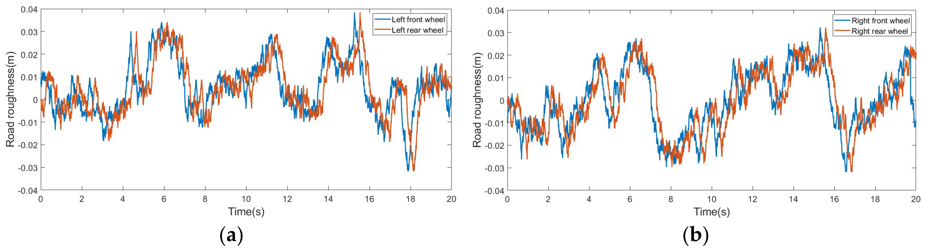
2.3.1. Pavement Modeling

(1) C-Class Random Pavement

The road excitation model describes the degree of roughness of the road surface. In the simulation analysis of the road surface model, there are two approaches to converting the spatial model of the road surface into either a frequency-domain model or a time-domain model. Using the mathematical model of filtered white noise, the time domain model of road roughness [21] can be formulated as follows:

$$\dot{q}(t)=-2\pi n_{1}uq(t)+2\pi n_{0}w\sqrt{Gq(n_0)v}$$

(23)

where $\dot{q}$ represents the vertical velocity spectrum of road roughness and the reciprocal of displacement; $v$ is the vehicle speed, with 54 km/h (15 m/s) adopted in this paper; $Gq\left(n_0\right)$ represents the road roughness; $n_1$ represents the lower cutoff spatial frequency, taken as 0.01 m⁻¹ in this paper; $n_0$ represents the reference spatial frequency, assigned a value of 0.1 m⁻¹; $Gq\left(n_0\right)$ represents the road roughness coefficient; the C-class pavement roughness coefficient of the pavement is $Gq\left(n_0\right)$ = 256 × 10⁻⁶ m³; and w is the unit of white noise.

Assuming that the vehicle moves smoothly along a straight path, it encounters different road surfaces on its left and right sides. Figure 5 illustrates the displacements of the front and rear wheels on both the left and right sides when the vehicle traverses a constructed C-class pavement. The velocity spectrum of this pavement resembles white noise, with vertical irregularities ranging primarily between −20 mm and 20 mm.

(2) Convex Pavement

When a vehicle is driving on a road, it will encounter raised obstacles, resulting in instantaneous and strong impacts, which will affect the ride’s comfort. Following the specifications outlined in the GB/T5902-1986 standard in the “Automobile Ride Comfort Pulse Input Driving Test Method”, the triangle bump pulse excitation is specifically defined as follows [22]:

$$q(t)=\left\{\begin{array}{c}2{\displaystyle \frac{H}{B}}v(t-t_1),t_1\le t\le t_2\\ 2{\displaystyle \frac{H}{B}}\left(B-v(t-t_1)\right),t_1+t_2\le t\le 2t_2\\ 0,else\end{array}\right.$$

(24)

In the formula, $H$ = 0.06 m, where $H$ is the height of the triangular convex block, $B$ = 0.4 m, where $B$ is the width of the convex block, and $v$ = 36 km/h (10 m/s), where $v$ is the speed of the vehicle.

The left wheel is impacted by the convex block at 1 s, and the right wheel is impacted by the convex block at 3 s. The displacement of the tire with the constructed triangular bump is shown in Figure 6.

2.3.2. Suspension Model

To verify the control effect of the proposed controller for ESO-MPC, two working conditions of C-class random pavement and convex pavement were established, and the traditional passive hydropneumatic suspension was compared. The parameters used for selecting a specific heavy-duty vehicle are presented in

Table 1. Parameters of special vehicles.

Parameter	Parameter Value
Sprung mass	35,000 kg
Pitch moment of inertia	2.14 × 106 kgm2
Roll moment of inertia	3.27 × 106 kgm2
Front axle’s unsprung mass	1350 kg
Rear axle’s unsprung mass	1650 kg
Tire’s equivalent stiffness	2 × 106 N/m
Wheelbase	4 m
Distance from front wheels to center of mass	2.2 m
Distance from rear wheels to center of mass	1.8 m
Front wheel’s gauge	1.6 m
Rear wheel’s gauge	1.45 m

. The Simulink simulation model comprising the pneumatic suspension, the ESO state observer, the controller for MPC, and the road model is shown in Figure 7.

3. Results and Discussion

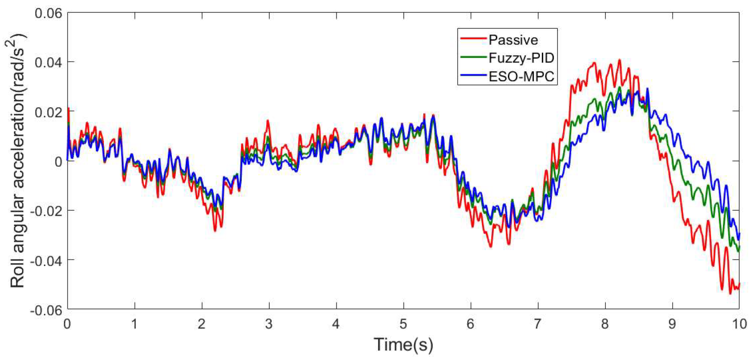
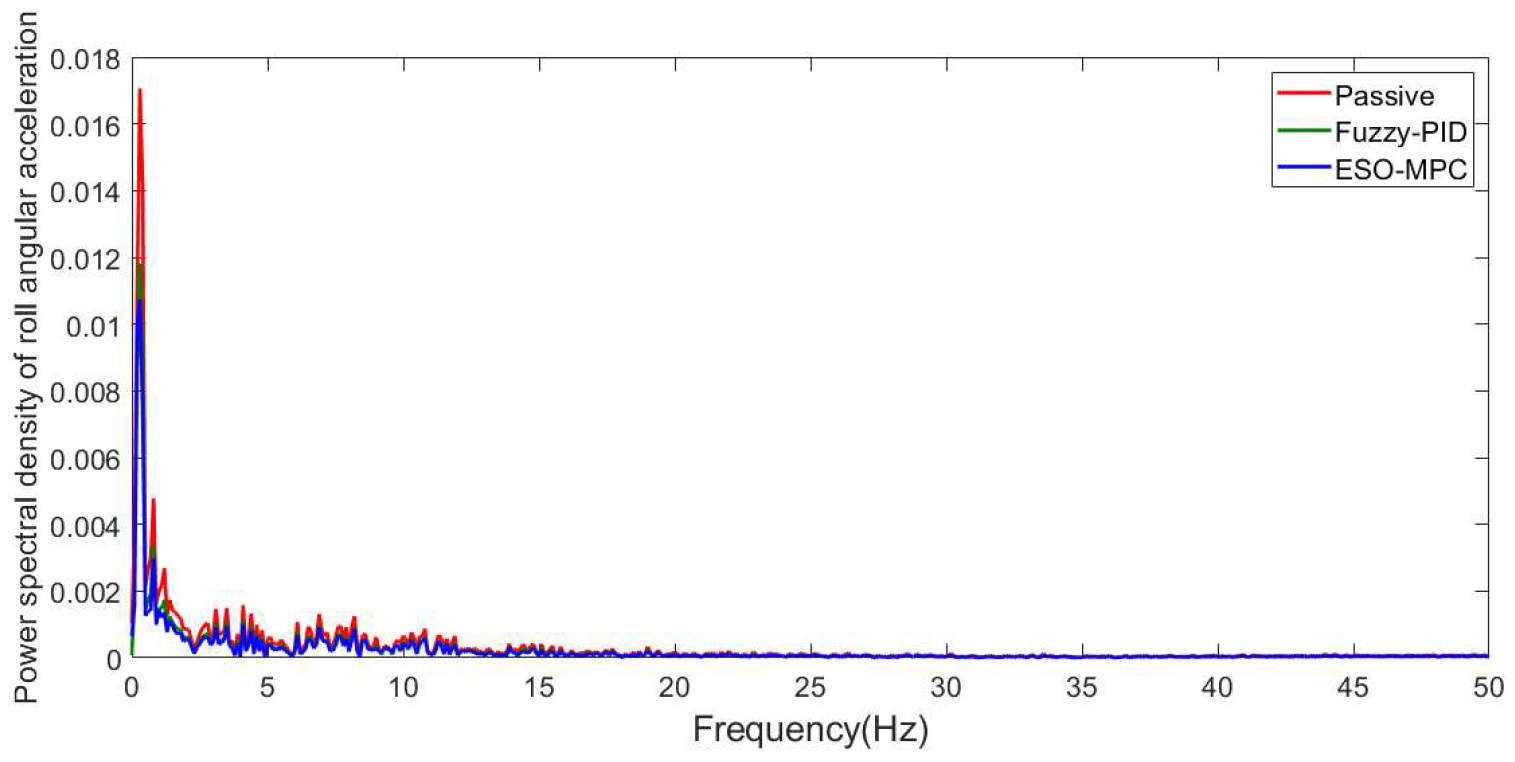
3.1. C-Class Random Pavement

For a C-class pavement, Figure 8 shows the comparison of the vehicle body’s vertical acceleration before and after applying control measures. Figure 9 presents a comparison of the power spectra of the vehicle body’s vertical acceleration before and after control. Figure 10 shows the comparison of the vehicle body’s pitch-angular acceleration before and after control, while Figure 11 depicts the comparison of its power spectrum. Figure 12 shows the comparison of the vehicle body’s roll-angle acceleration before and after control, and Figure 13 shows the comparison of its power spectrum.

The figures indicate that the vibration control modes remained largely consistent across the same road surface. Following the adoption of ESO-MPC and fuzzy PID control, there was a noticeable reduction in the amplitudes of the suspension’s vertical vibration acceleration, pitch-angle acceleration, and side-inclination acceleration in both the time and frequency domains. This led to an improvement in the ride comfort of the suspension.

Table 2. C-class random pavement index root mean square statistics.

Index	Passivity	Fuzzy PID	Reduction	ESO-MPC	Reduction
Vertical acceleration (m/s2)	0.26502	0.25021	5.588%	0.2154	18.725%
Pitch-angle acceleration (rad/s2)	0.045875	0.042206	7.99%	0.034537	24.716%
Roll-angle acceleration (rad/s2)	0.040128	0.033891	15.542%	0.029654	26.102%

presents the RMS indices of the evaluation indicators before and after control, revealing improvements across three key metrics: vertical acceleration, pitch-angle acceleration, and side-angle acceleration. After ESO-MPC was adopted, the vertical acceleration reduction was 18.7%, the pitch acceleration reduction was 24.7%, and the roll-angle acceleration reduction was 26.1%. After fuzzy PID control was adopted, the vertical acceleration reduction was 5.59%, the pitch-angle acceleration reduction was 7.99%, and the roll-angle acceleration reduction was 15.54%. The simulation results demonstrated that the ESO-MPC algorithm had a better active control effect on the hydropneumatic suspension, verifying the effectiveness of the control.

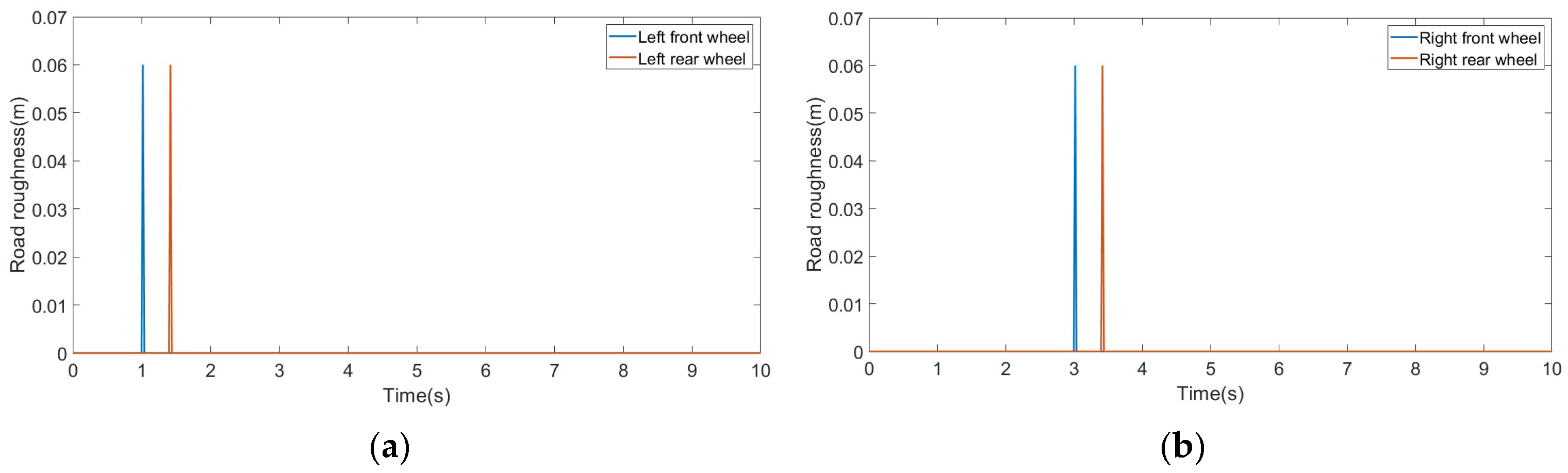
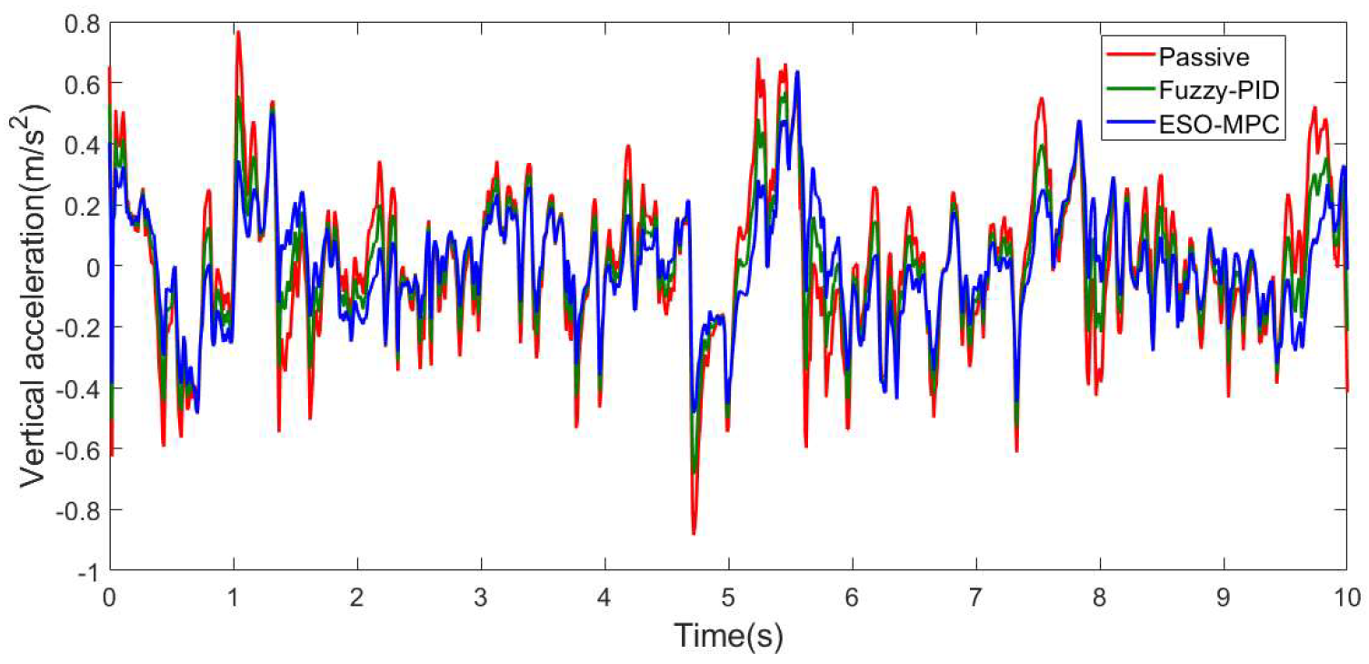
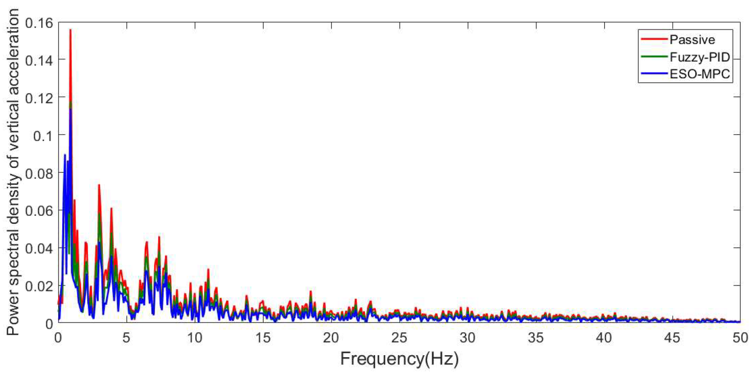
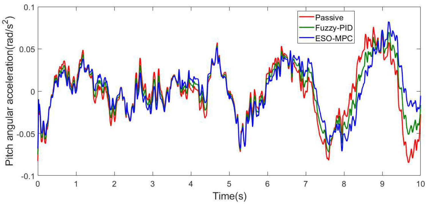
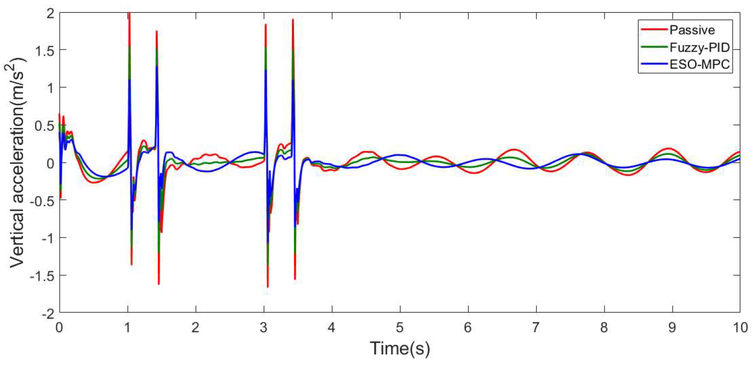
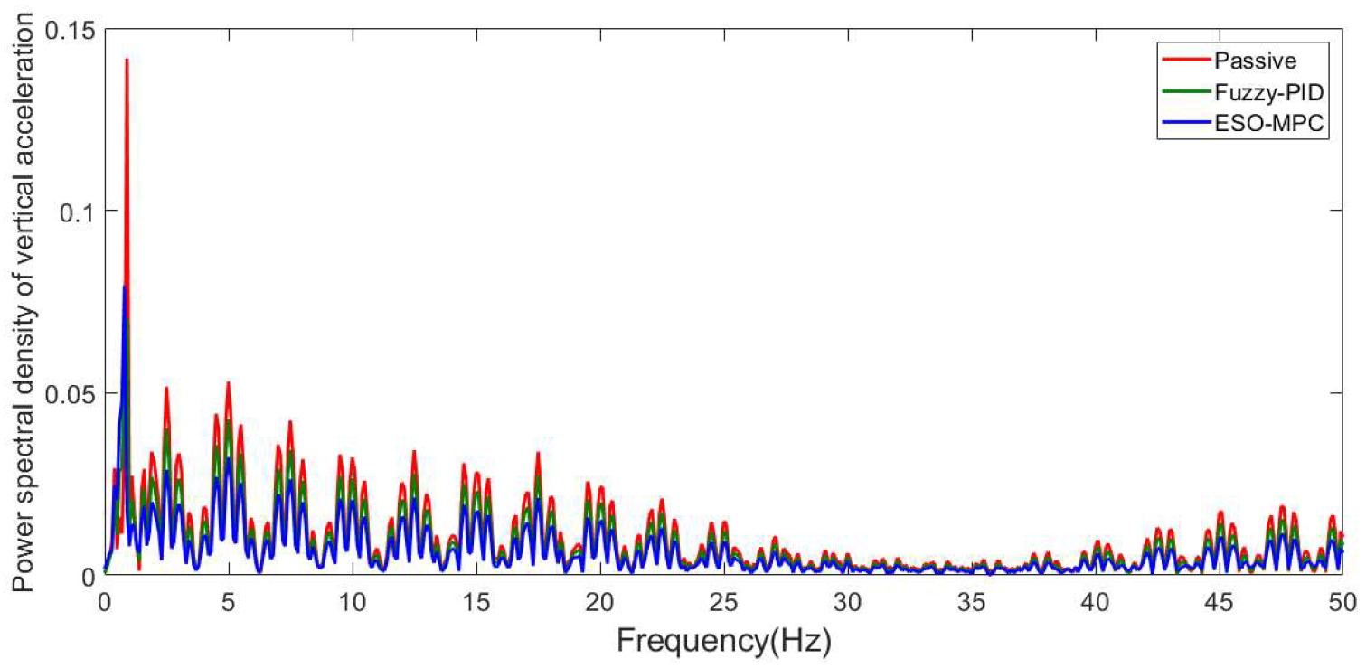
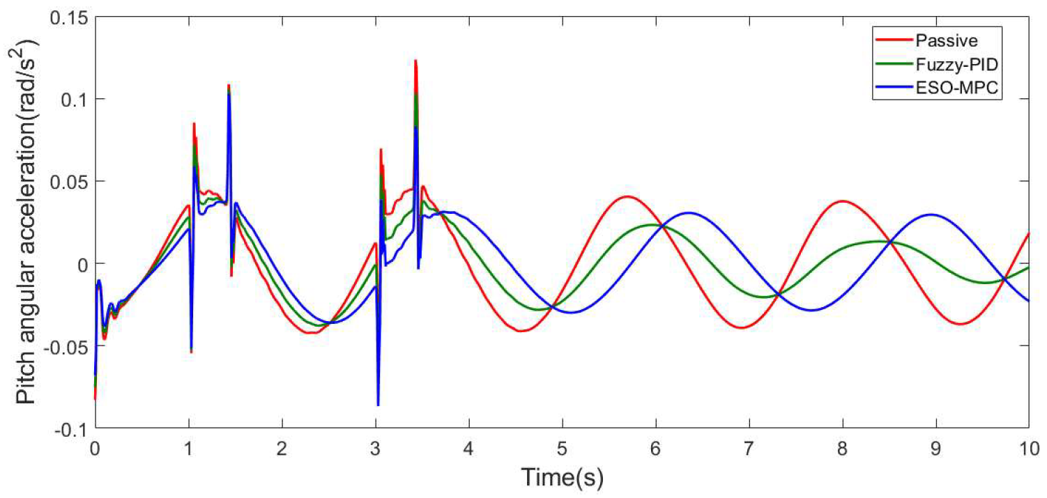
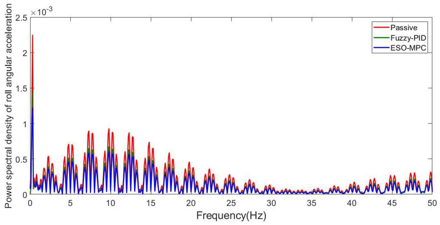
3.2. Convex Pavement

For a convex pavement, Figure 14 compares the vehicle body’s vertical acceleration before and after the implementation of control measures. Figure 15, in turn, shows the comparison of the power spectrum of the vehicle body’s vertical acceleration under the same conditions. Figure 16 shows the comparison of the vehicle body’s pitch angular acceleration before and after control. Figure 17 shows the corresponding comparison of its power spectrum. Figure 18 shows the comparison of the vehicle body’s roll-angle acceleration before and after control, and Figure 19 shows the comparison of its power spectrum.

The results indicate that the vibration control modes remained consistent across the same road surface. Upon implementing ESO-MPC and fuzzy PID control, there was a significant reduction in the amplitudes of the suspension’s vertical vibration acceleration, pitch-angle acceleration, and side-inclination acceleration in both the time and frequency domains. This reduction translated into an enhancement in the ride comfort of the suspension.

Table 3. Convex pavement index root mean square statistics.

Index	Passivity	Fuzzy PID	Reduction	ESO-MPC	Reduction
Vertical acceleration (m/s2)	0.23744	0.20410	14.041%	0.15076	36.507%
Pitch-angle acceleration (rad/s2)	0.029651	0.026508	10.599%	0.023365	21.199%
Roll-angle acceleration (rad/s2)	0.0044827	0.0041275	7.923%	0.0036723	18.079%

presents the RMS indices of the evaluation indicators before and after control, highlighting improvements in three key areas: vertical acceleration, pitch-angle acceleration, and side-angle acceleration. After ESO-MPC was adopted, the vertical acceleration reduction was 36.5%, the pitch-angle acceleration reduction was 21.2%, and the roll-angle acceleration reduction was 18.1%. After fuzzy PID control was adopted, the vertical acceleration reduction was 14.04%, the pitch-angle acceleration reduction was 10.6%, and the roll-angle acceleration reduction was 7.92%. The above results demonstrate that the ESO-MPC algorithm had a better active control effect on the hydropneumatic suspension, verifying the effectiveness of the control.

3.3. Discussion

The simulation system could still operate normally under different responses without introducing oscillations. Compared with fuzzy PID, ESO-MPC had a better control performance. In the diagram of the simulation results, ESO-MPC had no time delay; as ESO-MPC usually requires more complex calculations, this might have been due to simplifying the model and reducing the number of computations. Fuzzy PID is usually suitable for simple nonlinear systems, which might have been one of the reasons for its poor control performance. Compared with fuzzy PID, ESO-MPC had stronger disturbance resistance because it estimated the unmodeled dynamics and external disturbances of the system through an extended state observer (ESO). On random road surfaces, the ESO-MPC effect was significantly improved, whereas the fuzzy PID control’s effect was far inferior. However, on convex road surfaces, the improvement in fuzzy PID increased, indicating that ESO-MPC had a high control performance for random inputs.

4. Conclusions

To address the problems of the weak adaptability of passive X-type interconnected hydropneumatic suspensions to different road surfaces and the poor effect of the traditional single-control mode, an active controller of hydropneumatic suspensions based on ESO and MPC was designed. On the basis of the analysis of X-type interconnected hydropneumatic suspensions and the seven-degree-of-freedom suspension model, a three-degree-of-freedom linearized hydropneumatic suspension model with disturbance was established. The disturbance was analyzed, the disturbed ESO extended state observer was established, and, utilizing the linearized state space model as its foundation, the controller for ESO-MPC was constructed from MPC, thereby notably enhancing the performance of the heavy-duty truck’s suspension system.

In the C-class random road simulation verification, compared to passive suspension, active suspension using the controller for ESO-MPC reduced the vertical acceleration, pitch acceleration, and roll acceleration by 18.7%, 24.7%, and 26.1%, respectively. After fuzzy PID control, the vertical acceleration, pitch acceleration, and roll acceleration were reduced by 5.59%, 7.99%, and 15.54%, respectively. Simulation verification on a convex road surface showed that active suspension using the controller for ESO-MPC reduced the vertical acceleration of the vehicle by 36.5%, the pitch acceleration by 21.2%, and the roll acceleration by 18.1% compared to passive suspension. After adopting fuzzy PID control, the vertical acceleration, pitch acceleration, and roll acceleration were reduced by 14.04%, 10.6%, and 7.92%, respectively. The results indicated that the control effect of ESO-MPC was superior to that of fuzzy PID.

The ESO-MPC algorithm has better active control on hydropneumatic suspensions, especially on random road surfaces, where the control effect is more obvious than with fuzzy PID, achieving the precise control of X-type interconnected hydropneumatic suspension systems and improving the smoothness and stability of heavy-duty special vehicles.

References

1. Shi, Y.X.; Liu, T.H.; Yue, Z.S.; Cao, C.S.; Dou, B.; Zhao, H.H.; Yang, J.H. Study on Compound Control Method of Active Hydropneumatic Suspension of Mining Wide-body Vehicle. Mach. Tool Hydraul. 2023, 51, 173–179. [Google Scholar]
2. Zhang, J.; Li, S.; Shi, Y. Research on the performance of a special vehicle active hydro-pneumatic suspension. Manuf. Autom. 2018, 40, 43–49. [Google Scholar]
3. Nguyen, D.N.; Nguyen, T.A.; Dang, N.D. A novel sliding mode control al-gorithm for an active suspension system considering with the hydraulic actuator. Lat. Am. J. Solids Struct. 2022, 19, e424. [Google Scholar] [CrossRef]
4. Sathishkumar, P.; Wang, R.; Yang, L.; Thiyagarajan, J. Trajectory control for tire burst vehicle using thestandalone and roll interconnected active suspensions with safety-comfort controlstrategy. Mech. Syst. Signal Process. 2020, 142, 106776. [Google Scholar] [CrossRef]
5. Gokul, P.S.; Malar, M.K. A contemporary adaptive air suspension using LQR control for passenger vehicles. ISA Trans. 2019, 93, 244–254. [Google Scholar]
6. Yang, Q.; Zhou, K.; Zhang, W.; Xu, X.; Yuan, C. Fuzzy-PID Control on Semi-active Air Suspension. Trans. Chin. Soc. Agric. Mach. 2008, 39, 24–29. [Google Scholar]
7. Caponetto, R.; Diamante, O.; Fargione, G.; Risitano, A.; Tringali, D. A soft computing approach to fuzzy sky-hook control of semiactive suspension. IEEE Trans. Control Syst. Technol. 2003, 11, 786–798. [Google Scholar] [CrossRef]
8. Zhang, J. Dynamic Characteristics and Control Method Investigation of Hydraulically Interconnected Suspension for Mining Vehicles. Ph.D. Thesis, Hunan University, Changsha, China, 2018. [Google Scholar]
9. Xu, X.; Zhou, X.; Ma, Y.; Zhang, J.; Wan, H.; Chen, L. Microgrid Operation Controller Based on Active Disturbance Rejection Control Technology. High Volt. Technol. 2016, 42, 3336–3346. [Google Scholar] [CrossRef]
10. Di Cairano, S.; Bemporad, A. Model Predictive Control Tuning by Controller Matching. IEEE Trans. Autom. Control. 2010, 55, 185–190. [Google Scholar] [CrossRef]
11. Zhang, R.; Yu, L.; Liu, A.; Zhang, W.A. Distribute Model Predictive Control for Large-scale Systems with Multi-Rate Sampling. In Proceedings of the 33th Chinese Control Conference, Nanjing, China, 28–30 July 2014; pp. 1401–1406. [Google Scholar]
12. GK, V.S.; Fusic, J.; Ramesh, H. Advanced control strategies for Servo motors: Analysis of PID, FUZZY-PID and MPC with cuk converter integration. In Proceedings of the 2023 International Conference on Energy, Materials and Communication Engineering: International Conference on Energy, Materials and Communication Engineering (ICEMCE), Madurai, India, 14–15 December 2023; pp. 1–6. [Google Scholar]
13. Zinage, S.; Somayajula, A. A comparative study of different active heave compensation approaches. Ocean Syst. Eng. 2020, 10, 373–397. [Google Scholar] [CrossRef]
14. Zhang, X.; Li, Y.; Wang, Z. Integration of LQR and ESO for Enhanced Control Performance in Uncertain Systems. J. Control. Sci. Eng. 2022, 10, 123–135. [Google Scholar]
15. Wang, J.; Li, H.; Chen, L. A Novel ESO-based MPC Strategy for Industrial Motion Control Systems. IEEE Trans. Ind. Electron. 2021, 68, 4567–4578. [Google Scholar]
16. Wu, X.; Zhou, B.; Wen, G. A study on anti-roll control of half-car model active interconnected suspension with consideration of actuator dynamics. Vib. Shock 2017, 36, 150–154. [Google Scholar] [CrossRef]
17. Chen, W.; Xiao, H.; Wang, Q.; Zhao, L.; Zhu, M. Integrated Vehicle Dynamics and Control; Wiley: Hoboken, NJ, USA, 2016. [Google Scholar]
18. Liang, Y.; Chen, X.; Xu, R. Research on Longitudinal Landing Track Control Technology of Carrier-based Aircraft. In Proceedings of the 2020 Chinese Control And Decision Conference (CCDC), Hefei, China, 22–24 August 2020. [Google Scholar]
19. Xu, H.; Zhao, Y.; Wang, Q.; Lin, F.; Pi, W. Decoupling control of active suspension and four-wheel steering based on Backstepping-ADRC with mechanical elastic wheel. Proc. Inst. Mech. Eng. Part D J. Automob. Eng. 2021, 236, 2356–2373. [Google Scholar] [CrossRef]
20. Liu, Y.; Wang, S.; Li, G.; Mao, B.; Dong, Z.; Li, D. Optimal parameter identification of hydro-pneumatic suspension for mine cars. Int. J. Simul. Multidisci. Des. Optim. 2024, 15, 26. [Google Scholar] [CrossRef]
21. Doe, J.; Smith, J. Modeling of Road Surface Profiles Using Filtered White Noise. J. Veh. Syst. Dyn. 2020, 58, 456–470. [Google Scholar]
22. GB/T 5902-1986; Test Method for Automobile Ride Comfort by Random Input Running. China Standards Press: Beijing, China, 1986.
Figure 1. Schematic diagram of X-type interconnected hydropneumatic suspension.
Applsci 15 03041 g001
Figure 2. Active X-type interconnected hydropneumatic suspension structure: 1—hydraulic pump; 2—safety valve; 3—servo valve; and 4—angle sensor.
Applsci 15 03041 g002
Figure 3. Seven-DOF model.
Applsci 15 03041 g003
Figure 4. ESO-MPC force controller algorithm flowchart.
Applsci 15 03041 g004
Figure 5. C−class random pavement: (a) left and (b) right.
Applsci 15 03041 g005
Figure 6. Convex pavement: (a) left and (b) right.
Applsci 15 03041 g006
Figure 7. Active ESO-MPC model for interconnected hydropneumatic suspensions.
Applsci 15 03041 g007
Figure 8. Vertical acceleration on C−class random pavement.
Applsci 15 03041 g008
Figure 9. Vertical acceleration power spectra on C−class random pavement.
Applsci 15 03041 g009
Figure 10. Vehicle pitch acceleration on C−class random pavement.
Applsci 15 03041 g010
Figure 11. Power spectrum of body pitch angular acceleration on C−class random pavement.
Applsci 15 03041 g011
Figure 12. Vehicle roll−angle acceleration on C−class random pavement.
Applsci 15 03041 g012
Figure 13. Power spectrum of body roll−angle acceleration on C−class random pavement.
Applsci 15 03041 g013
Figure 14. Vertical acceleration of the vehicle on convex pavement.
Applsci 15 03041 g014
Figure 15. Power spectrum of the vertical acceleration on convex pavement.
Applsci 15 03041 g015
Figure 16. Body pitch−angle acceleration on convex pavement.
Applsci 15 03041 g016
Figure 17. Power spectra of body pitch−angle acceleration on convex pavement.
Applsci 15 03041 g017
Figure 18. Body roll−angle acceleration on convex pavement.
Applsci 15 03041 g018
Figure 19. Power spectra of body roll−angle acceleration on convex pavement.
Applsci 15 03041 g019