The Impact of Squeeze Film Damper and Support Nonlinear Forces on the Dynamic Response of High-Speed Flexible Rotors

Abstract

To investigate the nonlinear dynamic response of rotor systems, a finite element model of the squeeze film damper-rotor system was established. With the Euler–Bernoulli beam rotor model, the nonlinear oil film forces of the squeeze film damper (SFD) and the nonlinear restoring forces of the supports are applied as external loads to the support nodes using the finite element method. The Newmark Beta method was used to solve it, and the nonlinear dynamic response of the rotor was analyzed using frequency–response curves, time-domain response diagrams, and shaft centerline trajectory diagrams. The effects of different oil film gaps and support restoring force coefficients on the rotor response were examined. The results show that the coupling effect of the two nonlinear forces is the superposition of their individual effects; the two nonlinear forces have a significant impact on the rotor response amplitude, and appropriate parameter selection and installation positions can reduce the amplitude by 19%; and finally, among the two nonlinear forces, the SFD nonlinear oil film force mainly affects the amplitude, while the support nonlinear restoring force affects both the amplitude and frequency.

1. Introduction

Aero-engines, known as the “crown jewels of modern industry”, play a crucial role in the development of aviation technology. The rotor-support system in aero-engines is its core component, and its performance directly affects the stable operation of the aero-engine under extreme conditions such as high temperature, high pressure, high speed, and high load, and it also plays a key role in the overall performance of the engine. Vibration damping methods can be implemented through active [1,2] or passive approaches. The excellent vibration reduction and stability enhancement characteristics of the squeeze film damper (SFD) have led to its widespread application in aero-engines [3]. The difficulty in studying the vibration characteristics of the rotor-support system lies in the nonlinear forces used in the elastic support and the SFD, especially the highly nonlinear characteristics of the SFD oil film force. Therefore, conventional linear analysis methods cannot be used to analyze the rotor system containing SFD. How to balance calculation speed and accuracy for the response analysis of the nonlinear rotor-support system is a problem worth studying.

Vance et al. [3,4,5,6] studied the mechanical mechanism and vibration reduction characteristics of SFD. Yuwei Zhang et al. [7] established a finite element model of a dual-rotor system incorporating a squeeze film damper with rigid supports (SDERSFD) to investigate its nonlinear dynamic characteristics and vibration attenuation performance. Yufei Xu et al. [8] developed a coupled dynamic model of the rotor-SFD system accounting for nonlinear oil film forces in SFDs, validated through bench-test measurements of typical vibration responses. Xiaomin Yang et al. [9] proposed an integrated model of an elastic ring squeeze film damper (ERSFD) combined with high-speed ball bearings, using cage stiffness and rotor speed as variables. Numerical simulations were conducted to analyze steady-state and transient responses of journal bearings, while experimental measurements confirmed that low cage stiffness combined with high rotor speeds effectively stabilized the journal and suppressed vibrations. Wujiu Pan et al. [10] systematically analyzed the effects of different parameters (bifurcation diagrams, three-dimensional spectrum plots, and orbit plots) on system dynamics, including bearing clearance and interjournal clearance. Defaye et al. [11] experimentally investigated the influence of two dual-rotor configurations and three types of interjournal ball-bearing SFDs on vibration attenuation and nonlinear behavior. Weimin Wang et al. [12] revealed the dynamic coupling mechanism between flexible casings and SFDs during flight maneuvers.

Longkai Wang et al. [13] introduced the effect of internal resistance on nonlinear restoring forces and analyzed the bi-stable mechanism using bifurcation diagrams, Lyapunov exponents, and Poincaré sections. Through coupling analysis of oil film forces and internal resistance, they revealed the suppression of bi-stable phenomena by SFDs. Haibiao Zhang et al. [14] investigated an aero-engine rotor system based on dynamic similarity principles and proposed a simplified model to reveal its vibration response patterns. Their study focused on the vibration attenuation effect of SFDs, and the results showed that reverse-phase imbalanced distributions could be effectively suppressed by SFDs. Hubiao Tang et al. [15] used SAMCEF software to investigate the impact of elastic support stiffness on rotor critical speeds. Dayi Zhang et al. [16] combined finite element method with the vibration mode selection technique to predict critical speeds of twin-rotor systems. Zhanchi Liu [17] studied the effect of static eccentricity on the vibration reduction characteristics of the squeeze film damper, proving that the working characteristics of the squeeze film damper are related to its eccentricity ratio, and provided the linear working range of the squeeze film damper. The oil film force and damping models of the squeeze film damper under different oil film conditions in the long bearing theory and short bearing theory were established. Xinxing Ma et al. [18] conducted a comparative analysis of SFDs on nonlinear dynamic behaviors in roller-bearing-supported dual-rotor systems, demonstrating that SFDs can effectively suppress amplitude hopping under unbalanced excitation of dual rotors. Hailun Zhou et al. [19] developed a dynamic model of a rotor system supported by roller bearings and a floating ring squeeze film damper (FSFD), revealing that FSFDs significantly reduce bi-stable responses in the system. Tian Gao et al. [20] established a flexible asymmetric rotor system model incorporating nonlinear support interactions between rollers, bearings, and SFDs. Their results highlighted significant nonlinear features such as bi-stable phenomena, amplitude hopping, and desynchronized vibrations arising from the nonlinear coupling among the rotor, bearings, and SFDs.

Existing research has addressed nonlinear phenomena caused by SFDs and critical speed calculations of rotors, yet it remains unclear how the imbalance response of rotors differs under the influence of nonlinear forces versus linear ones. Due to the difficulty in modeling the nonlinear dynamic characteristics of SFDs in support structures, establishing a precise analytical model to reveal the parametric influence laws of complex vibration behaviors remains challenging. This paper proposes a finite element model to investigate the impact of nonlinear forces on the dynamic characteristics of rotors.

This paper employs the Euler–Bernoulli beam rotor model and establishes a dynamic model of the rotor-support system using the finite element method (FEM). Two nonlinear forces are applied to the model as external loads, allowing for their adjustment and removal. The Newmark β method is introduced to solve the time-domain response of the rotor system, facilitating the investigation of the nonlinear forces’ impact on the system’s dynamic characteristics. Initially, the nonlinear forces are neglected to compute the rotor response under no external excitation. Subsequently, the SFD nonlinear oil film force and the support nonlinear restoring force are added separately to analyze their individual effects on the rotor response. Finally, both nonlinear forces are coupled and applied to study their synergistic influence on the system’s behavior.

2. Control Equations for Euler–Bernoulli Rotor

This chapter presents the derivation of the vibration equations for the rotor-support system based on the free vibration equation of the Euler–Bernoulli beam, incorporating the squeeze film damper (SFD) oil film force and support restoring force. Initially, the free vibration equation for the beam element is derived, followed by the derivation of the stiffness matrix, mass matrix, and gyroscopic matrix for the concentrated mass element, SFD element, and support element. Finally, all matrices are assembled into the overall stiffness matrix, which serves as the foundation for subsequent calculations.

2.1. Free Vibration Equation of the Beam Element

The control equation for the Euler–Bernoulli beam under free vibration conditions is derived, assuming that the beam segment is an isotropic circular cross-section with a uniform cross-sectional area throughout; the material of the beam segment is an elastic material with an elastic modulus denoted as E.

The (generalized) displacement of the beam element’s centerline nodes can be expressed in the following form:

$$v,w$$

(1)

$${\theta }_y=-{\displaystyle \frac{\mathsf{\partial }w}{\mathsf{\partial }x}},{\theta }_z={\displaystyle \frac{\mathsf{\partial }v}{\mathsf{\partial }x}}$$

(2)

The displacement field can be expressed as

$$u_x=-y{\displaystyle \frac{\mathsf{\partial }v}{\mathsf{\partial }x}}+z{\displaystyle \frac{\mathsf{\partial }w}{\mathsf{\partial }x}}$$

(3)

Consequently, the coordinate representation of the micro-element $dA$ of the beam element in the moving coordinate system is given by

$$\left\{\begin{array}{c}\xi \\ \eta \\ \zeta \end{array}\right\}=R_x{R}_y{R}_z\left(\left\{\begin{array}{c}x\\ y\\ z\end{array}\right\}-\left\{\begin{array}{c}0\\ v\\ w\end{array}\right\}\right)$$

(4)

R_x, R_y, and R_z represent the fundamental rotation matrices about the X, Y, and Z axes.

Utilizing transformation, the coordinates of the micro-element $dA$ in the inertial coordinate system are delineated as

$$\left\{\begin{array}{c}x\\ y\\ z\end{array}\right\}=R_z^T{R}_y^T{R}_x^T\left\{\begin{array}{c}\xi \\ \eta \\ \zeta \end{array}\right\}+\left\{\begin{array}{c}0\\ v\\ w\end{array}\right\}$$

(5)

The stress and strain within the beam element are hereby illustrated:

In the equation, $v,w$ represent the displacements of the micro-element $dA$ in the x and y directions, respectively, while E denotes the elastic modulus.

$${\epsilon }_{xx}=-y{\displaystyle \frac{{\mathsf{\partial }}^{2}v}{\mathsf{\partial }{x}^2}}+z{\displaystyle \frac{{\mathsf{\partial }}^{2}w}{\mathsf{\partial }{x}^2}}$$

(6)

$${\sigma }_{xx}=E{\left(-y{\displaystyle \frac{{\mathsf{\partial }}^{2}v}{\mathsf{\partial }{x}^2}}+z{\displaystyle \frac{{\mathsf{\partial }}^{2}w}{\mathsf{\partial }{x}^2}}\right)}^2$$

(7)

Consequently, the elastic potential energy of the micro-element $dA$ is expressed as

$$dU={\displaystyle {\int }_A\frac{1}{2}{\sigma }_{xx}{\epsilon }_{xx}dA}={\displaystyle \frac{1}{2}}{\displaystyle {\int }_{A}E{\left(-y\frac{{\mathsf{\partial }}^{2}v}{\mathsf{\partial }{x}^2}+z\frac{{\mathsf{\partial }}^{2}w}{\mathsf{\partial }{x}^2}\right)}^{2}dA}={\displaystyle \frac{1}{2}}EI\left[{\left({\displaystyle \frac{{\mathsf{\partial }}^{2}v}{\mathsf{\partial }{x}^2}}\right)}^2+{\left({\displaystyle \frac{{\mathsf{\partial }}^{2}w}{\mathsf{\partial }{x}^2}}\right)}^2\right]$$

(8)

$$U={\displaystyle \frac{1}{2}}{\displaystyle {\int }_0^{L}EI\left[{\left(\frac{{\mathsf{\partial }}^{2}v}{\mathsf{\partial }{x}^2}\right)}^2+{\left(\frac{{\mathsf{\partial }}^{2}w}{\mathsf{\partial }{x}^2}\right)}^2\right]dx}$$

(9)

$$\begin{array}{c}\delta U={\displaystyle {\int }_0^{L}EI\left[\frac{{\mathsf{\partial }}^{2}v}{\mathsf{\partial }{x}^2}\delta \left(\frac{{\mathsf{\partial }}^{2}v}{\mathsf{\partial }{x}^2}\right)+\frac{{\mathsf{\partial }}^{2}w}{\mathsf{\partial }{x}^2}\delta \left(\frac{{\mathsf{\partial }}^{2}w}{\mathsf{\partial }{x}^2}\right)\right]dx}\hfill \\ ={\displaystyle {\int }_0^{L}EI\frac{{\mathsf{\partial }}^{2}v}{\mathsf{\partial }{x}^2}d\left(\frac{\mathsf{\partial }\delta v}{\mathsf{\partial }x}\right)}+{\displaystyle {\int }_0^{L}EI\frac{{\mathsf{\partial }}^{2}w}{\mathsf{\partial }{x}^2}d\left(\frac{\mathsf{\partial }\delta w}{\mathsf{\partial }x}\right)}\hfill \\ =EI{\displaystyle \frac{{\mathsf{\partial }}^{2}v}{\mathsf{\partial }{x}^2}}\delta \left({\displaystyle \frac{\mathsf{\partial }v}{\mathsf{\partial }x}}\right)-EI{\displaystyle \frac{{\mathsf{\partial }}^{3}v}{\mathsf{\partial }{x}^3}}\left(\delta v\right)+EI{\displaystyle \frac{{\mathsf{\partial }}^{2}w}{\mathsf{\partial }{x}^2}}\delta \left({\displaystyle \frac{\mathsf{\partial }w}{\mathsf{\partial }x}}\right)-EI{\displaystyle \frac{{\mathsf{\partial }}^{3}w}{\mathsf{\partial }{x}^3}}\left(\delta w\right)\hfill \\ \hspace{1em} +{\displaystyle {\int }_0^{L}EI\frac{{\mathsf{\partial }}^{4}v}{\mathsf{\partial }{x}^4}\delta vdx}+{\displaystyle {\int }_0^{L}EI\frac{{\mathsf{\partial }}^{4}w}{\mathsf{\partial }{x}^4}\delta wdx}\hfill \end{array}$$

(10)

Examining the micro-element $dA$, its coordinates in the moving coordinate system $O\xi \eta \zeta$ are $\left(0,\eta ,\zeta \right)$, and in the inertial coordinate system $Oxyz$ are

$$\left\{\begin{array}{c}x\\ y\\ z\end{array}\right\}=R_z^T{R}_y^T{R}_x^T\left\{\begin{array}{c}0\\ \eta \\ \zeta \end{array}\right\}+\left\{\begin{array}{c}0\\ v\\ w\end{array}\right\}$$

(11)

Since the moving coordinate system is rigidly attached to the plane, the velocity of the micro-element in the moving coordinate system is zero. Consequently, in the inertial coordinate system, the velocity of the micro-element is derived as

$$\left\{\begin{array}{c}\dot{x}\\ \dot{y}\\ \dot{z}\end{array}\right\}={\displaystyle \frac{\mathsf{\partial }\left(R_x^T{R}_z^T{R}_y^T\right)}{\mathsf{\partial }t}}\left\{\begin{array}{c}0\\ \eta \\ \zeta \end{array}\right\}+\left\{\begin{array}{c}0\\ \dot{v}\\ \dot{w}\end{array}\right\}$$

(12)

Subsequently, we introduce the concept of

$$\sin \left({\theta }_x\right)~{\theta }_x,\sin \left({\theta }_y\right)~{\theta }_y,\cos \left({\theta }_x\right)~1,\cos \left({\theta }_y\right)~1$$

(13)

The kinetic energy of the micro-element can be formulated as

$$\begin{array}{cc}\hfill dT& ={\displaystyle {\int }_A\frac{1}{2}\rho \left({\dot{x}}^2+{\dot{y}}^2+{\dot{z}}^2\right)d\eta d\zeta }\hfill \\ & ={\displaystyle \frac{1}{2}}\left\{m{\dot{v}}^2+m{\dot{w}}^2-2J_p\Omega {\theta }_y{\dot{\theta }}_z+J_p{\Omega }^2+J_d{{\dot{\theta }}_y}^2+J_d{{\dot{\theta }}_z}^2\right\}\hfill \end{array}$$

(14)

$$T={\displaystyle \frac{1}{2}}{\displaystyle {\int }_0^L\left[m{\dot{v}}^2+m{\dot{w}}^2-2J_p\Omega {\theta }_y{\dot{\theta }}_z+J_p{\Omega }^2+J_d{{\dot{\theta }}_y}^2+J_d{{\dot{\theta }}_z}^2\right]dx}$$

(15)

Substituting the angle expressions ${\theta }_y=-{\displaystyle \frac{\mathsf{\partial }w}{\mathsf{\partial }x}},{\theta }_z={\displaystyle \frac{\mathsf{\partial }v}{\mathsf{\partial }x}}$ into the equation, we obtain

$$T=T={\displaystyle \frac{1}{2}}{\displaystyle {\int }_0^L\left[m{\dot{v}}^2+m{\dot{w}}^2+2J_p\Omega \frac{\mathsf{\partial }w}{\mathsf{\partial }x}\frac{\mathsf{\partial }\dot{v}}{\mathsf{\partial }x}+J_p{\Omega }^2+J_d{\left(\frac{\mathsf{\partial }\dot{w}}{\mathsf{\partial }x}\right)}^2+J_d{\left(\frac{\mathsf{\partial }\dot{v}}{\mathsf{\partial }x}\right)}^2\right]dx}$$

(16)

$$\begin{array}{l}\delta T={\displaystyle \frac{1}{2}}\delta {\displaystyle {\int }_0^L\left[m{\dot{v}}^2+m{\dot{w}}^2+2J_p\Omega \frac{\mathsf{\partial }w}{\mathsf{\partial }x}\frac{\mathsf{\partial }\dot{v}}{\mathsf{\partial }x}+J_p{\Omega }^2+J_d{\left(\frac{\mathsf{\partial }\dot{w}}{\mathsf{\partial }x}\right)}^2+J_d{\left(\frac{\mathsf{\partial }\dot{v}}{\mathsf{\partial }x}\right)}^2\right]dx}\\ ={\displaystyle {\int }_0^L\left[m\dot{v}\delta \dot{v}+m\dot{w}\delta \dot{w}+J_p\Omega \left(\frac{\mathsf{\partial }\dot{v}}{\mathsf{\partial }x}\delta \frac{\mathsf{\partial }w}{\mathsf{\partial }x}+\frac{\mathsf{\partial }w}{\mathsf{\partial }x}\delta \frac{\mathsf{\partial }\dot{v}}{\mathsf{\partial }x}\right)+J_d\frac{\mathsf{\partial }\dot{w}}{\mathsf{\partial }x}\delta \left(\frac{\mathsf{\partial }\dot{w}}{\mathsf{\partial }x}\right)+J_d\frac{\mathsf{\partial }\dot{v}}{\mathsf{\partial }x}\delta \left(\frac{\mathsf{\partial }\dot{v}}{\mathsf{\partial }x}\right)\right]dx}\\ ={\displaystyle {\int }_0^L\left[-m\ddot{v}\delta v-m\ddot{w}\delta w+J_p\Omega \left(-\frac{{\mathsf{\partial }}^2\dot{v}}{\mathsf{\partial }{x}^2}\delta w+\frac{{\mathsf{\partial }}^2\dot{w}}{\mathsf{\partial }{x}^2}\delta v\right)+J_d\frac{{\mathsf{\partial }}^2\ddot{w}}{\mathsf{\partial }{x}^2}\delta w+J_d\frac{{\mathsf{\partial }}^2\ddot{v}}{\mathsf{\partial }{x}^2}\delta v\right]dx}\end{array}$$

(17)

Hamilton’s principle is articulated as

$$\begin{array}{l}\delta {\displaystyle {\int }_{t_1}^{t_2}\left(T-U\right)dt}\\ =-{\displaystyle {\int }_0^L\left[\begin{array}{l}EI\frac{{\mathsf{\partial }}^{4}v}{\mathsf{\partial }{x}^4}\delta v+EI\frac{{\mathsf{\partial }}^{4}w}{\mathsf{\partial }{x}^4}\delta w+m\ddot{v}\delta v+m\ddot{w}\delta w\\ -J_p\Omega \left(-\frac{{\mathsf{\partial }}^2\dot{v}}{\mathsf{\partial }{x}^2}\delta w+\frac{{\mathsf{\partial }}^2\dot{w}}{\mathsf{\partial }{x}^2}\delta v\right)-J_d\frac{{\mathsf{\partial }}^2\ddot{w}}{\mathsf{\partial }{x}^2}\delta w-J_d\frac{{\mathsf{\partial }}^2\ddot{v}}{\mathsf{\partial }{x}^2}\delta v\end{array}\right]dx}\\ =-{\displaystyle {\int }_0^L\left[\begin{array}{l}\left(EI\frac{{\mathsf{\partial }}^{4}v}{\mathsf{\partial }{x}^4}+m\ddot{v}-J_p\Omega \frac{{\mathsf{\partial }}^2\dot{w}}{\mathsf{\partial }{x}^2}-J_d\frac{{\mathsf{\partial }}^2\ddot{v}}{\mathsf{\partial }{x}^2}\right)\delta v\\ +\left(EI\frac{{\mathsf{\partial }}^{4}w}{\mathsf{\partial }{x}^4}+m\ddot{w}+J_p\Omega \frac{{\mathsf{\partial }}^2\dot{v}}{\mathsf{\partial }{x}^2}-J_d\frac{{\mathsf{\partial }}^2\ddot{w}}{\mathsf{\partial }{x}^2}\right)\delta w\end{array}\right]dx}\end{array}$$

(18)

Ultimately, the free vibration control equation for the beam element is derived as follows:

$$EI{\displaystyle \frac{{\mathsf{\partial }}^{4}v}{\mathsf{\partial }{x}^4}}+m\ddot{v}-J_p\Omega {\displaystyle \frac{{\mathsf{\partial }}^2\dot{w}}{\mathsf{\partial }{x}^2}}-J_d{\displaystyle \frac{{\mathsf{\partial }}^2\ddot{v}}{\mathsf{\partial }{x}^2}}=0$$

(19)

$$EI{\displaystyle \frac{{\mathsf{\partial }}^{4}w}{\mathsf{\partial }{x}^4}}+m\ddot{w}+J_p\Omega {\displaystyle \frac{{\mathsf{\partial }}^2\dot{v}}{\mathsf{\partial }{x}^2}}-J_d{\displaystyle \frac{{\mathsf{\partial }}^2\ddot{w}}{\mathsf{\partial }{x}^2}}=0$$

(20)

The weak form equation of the beam element’s control equation is given by

$${\displaystyle {\int }_{x_i}^{x_j}\left(EI\frac{{\mathsf{\partial }}^{4}v}{\mathsf{\partial }{x}^4}+m\ddot{v}-J_p\Omega \frac{{\mathsf{\partial }}^2\dot{w}}{\mathsf{\partial }{x}^2}-J_d\frac{{\mathsf{\partial }}^2\ddot{v}}{\mathsf{\partial }{x}^2}\right)\delta vdx}+{\displaystyle {\int }_{x_i}^{x_j}\left(EI\frac{{\mathsf{\partial }}^{4}w}{\mathsf{\partial }{x}^4}+m\ddot{w}+J_p\Omega \frac{{\mathsf{\partial }}^2\dot{v}}{\mathsf{\partial }{x}^2}-J_d\frac{{\mathsf{\partial }}^2\ddot{w}}{\mathsf{\partial }{x}^2}\right)\delta wdx}=0$$

(21)

where $\delta v$ and $\delta w$ represent the virtual displacements. Integrating the weak form equation by parts yields

$$\begin{array}{l}{\displaystyle {\int }_{x_i}^{x_j}\left(EI\frac{{\mathsf{\partial }}^{4}v}{\mathsf{\partial }{x}^4}\right)\delta vdx}=EI{\displaystyle \frac{{\mathsf{\partial }}^{3}v}{\mathsf{\partial }{x}^3}}{\left(\delta v\right)}_{x_i}^{x_j}-EI{\displaystyle \frac{{\mathsf{\partial }}^{2}v}{\mathsf{\partial }{x}^2}}\delta {\left({\displaystyle \frac{\mathsf{\partial }v}{\mathsf{\partial }x}}\right)}_{x_i}^{x_j}+{\displaystyle {\int }_{x_i}^{x_j}EI\frac{{\mathsf{\partial }}^{2}v}{\mathsf{\partial }{x}^2}\delta \left(\frac{{\mathsf{\partial }}^{2}v}{\mathsf{\partial }{x}^2}\right)dx}\\ {\displaystyle {\int }_{x_i}^{x_j}{J}_p\Omega \frac{{\mathsf{\partial }}^2\dot{w}}{\mathsf{\partial }{x}^2}\delta vdx}=J_p\Omega {\displaystyle \frac{\mathsf{\partial }\dot{w}}{\mathsf{\partial }x}}{\left(\delta v\right)}_{x_i}^{x_j}-{\displaystyle {\int }_{x_i}^{x_j}{J}_p\Omega \frac{\mathsf{\partial }\dot{w}}{\mathsf{\partial }x}\delta \left(\frac{\mathsf{\partial }v}{\mathsf{\partial }x}\right)dx}\\ {\displaystyle {\int }_{x_i}^{x_j}{J}_d\frac{{\mathsf{\partial }}^2\ddot{v}}{\mathsf{\partial }{x}^2}\delta vdx}=J_d{\displaystyle \frac{\mathsf{\partial }\ddot{v}}{\mathsf{\partial }x}}{\left(\delta v\right)}_{x_i}^{x_j}-{\displaystyle {\int }_{x_i}^{x_j}{J}_d\frac{\mathsf{\partial }\ddot{v}}{\mathsf{\partial }x}\delta \left(\frac{\mathsf{\partial }v}{\mathsf{\partial }x}\right)dx}\end{array}$$

(22)

The first integral is

$$\begin{array}{l}{\displaystyle {\int }_{x_i}^{x_j}\left(EI\frac{{\mathsf{\partial }}^{4}v}{\mathsf{\partial }{x}^4}+m\ddot{v}-J_p\Omega \frac{{\mathsf{\partial }}^2\dot{w}}{\mathsf{\partial }{x}^2}-J_d\frac{{\mathsf{\partial }}^2\ddot{v}}{\mathsf{\partial }{x}^2}\right)\delta vdx}\\ ={\displaystyle {\int }_{x_i}^{x_j}\left[EI\frac{{\mathsf{\partial }}^{2}v}{\mathsf{\partial }{x}^2}\delta \left(\frac{{\mathsf{\partial }}^{2}v}{\mathsf{\partial }{x}^2}\right)+m\ddot{v}\delta v+J_p\Omega \frac{\mathsf{\partial }\dot{w}}{\mathsf{\partial }x}\delta \left(\frac{\mathsf{\partial }v}{\mathsf{\partial }x}\right)+J_d\frac{\mathsf{\partial }\ddot{v}}{\mathsf{\partial }x}\delta \left(\frac{\mathsf{\partial }v}{\mathsf{\partial }x}\right)dx\right]dx}\end{array}$$

(23)

The intermediate step involves

$$\begin{array}{l}{\displaystyle {\int }_{x_i}^{x_j}\left(EI\frac{{\mathsf{\partial }}^{4}w}{\mathsf{\partial }{x}^4}\right)\delta wdx}=EI\frac{{\mathsf{\partial }}^{3}w}{\mathsf{\partial }{x}^3}{\left(\delta w\right)}_{x_i}^{x_j}-EI\frac{{\mathsf{\partial }}^{2}w}{\mathsf{\partial }{x}^2}\delta {\left(\frac{\mathsf{\partial }w}{\mathsf{\partial }x}\right)}_{x_i}^{x_j}+{\displaystyle {\int }_{x_i}^{x_j}EI\frac{{\mathsf{\partial }}^{2}w}{\mathsf{\partial }{x}^2}\delta \left(\frac{{\mathsf{\partial }}^{2}w}{\mathsf{\partial }{x}^2}\right)dx}\\ {\displaystyle {\int }_{x_i}^{x_j}{J}_p\Omega \frac{{\mathsf{\partial }}^2\dot{v}}{\mathsf{\partial }{x}^2}\delta wdx}=J_p\Omega \frac{\mathsf{\partial }\dot{v}}{\mathsf{\partial }x}{\left(\delta w\right)}_{x_i}^{x_j}-{\displaystyle {\int }_{x_i}^{x_j}{J}_p\Omega \frac{\mathsf{\partial }\dot{v}}{\mathsf{\partial }x}\delta \left(\frac{\mathsf{\partial }w}{\mathsf{\partial }x}\right)dx}\\ {\displaystyle {\int }_{x_i}^{x_j}{J}_d\frac{{\mathsf{\partial }}^2\ddot{w}}{\mathsf{\partial }{x}^2}\delta vdx}=J_d\frac{\mathsf{\partial }\ddot{w}}{\mathsf{\partial }x}{\left(\delta w\right)}_{x_i}^{x_j}-{\displaystyle {\int }_{x_i}^{x_j}{J}_d\frac{\mathsf{\partial }\ddot{w}}{\mathsf{\partial }x}\delta \left(\frac{\mathsf{\partial }w}{\mathsf{\partial }x}\right)dx}\end{array}$$

(24)

$$\begin{array}{l}{\displaystyle {\int }_{x_i}^{x_j}\left(EI\frac{{\mathsf{\partial }}^{4}w}{\mathsf{\partial }{x}^4}+m\ddot{w}+J_p\Omega \frac{{\mathsf{\partial }}^2\dot{v}}{\mathsf{\partial }{x}^2}-J_d\frac{{\mathsf{\partial }}^2\ddot{w}}{\mathsf{\partial }{x}^2}\right)\delta wdx}\\ ={\displaystyle {\int }_{x_i}^{x_j}\left[EI\frac{{\mathsf{\partial }}^{2}w}{\mathsf{\partial }{x}^2}\delta \left(\frac{{\mathsf{\partial }}^{2}w}{\mathsf{\partial }{x}^2}\right)+m\ddot{w}\delta w-J_p\Omega \frac{\mathsf{\partial }\dot{v}}{\mathsf{\partial }x}\delta \left(\frac{\mathsf{\partial }w}{\mathsf{\partial }x}\right)+{\displaystyle {\int }_{x_i}^{x_j}{J}_d\frac{\mathsf{\partial }\ddot{w}}{\mathsf{\partial }x}\delta \left(\frac{\mathsf{\partial }w}{\mathsf{\partial }x}\right)}\right]dx}\end{array}$$

(25)

Hereby, the weak form of the beam element’s control equation is rewritten as

$${\displaystyle {\int }_{x_i}^{x_j}\left[\begin{array}{l}EI\frac{{\mathsf{\partial }}^{2}v}{\mathsf{\partial }{x}^2}\delta \left(\frac{{\mathsf{\partial }}^{2}v}{\mathsf{\partial }{x}^2}\right)+m\ddot{v}\delta v+J_p\Omega \frac{\mathsf{\partial }\dot{w}}{\mathsf{\partial }x}\delta \left(\frac{\mathsf{\partial }v}{\mathsf{\partial }x}\right)+J_d\frac{\mathsf{\partial }\ddot{v}}{\mathsf{\partial }x}\delta \left(\frac{\mathsf{\partial }v}{\mathsf{\partial }x}\right)dx\\ +EI\frac{{\mathsf{\partial }}^{2}w}{\mathsf{\partial }{x}^2}\delta \left(\frac{{\mathsf{\partial }}^{2}w}{\mathsf{\partial }{x}^2}\right)+m\ddot{w}\delta w-J_p\Omega \frac{\mathsf{\partial }\dot{v}}{\mathsf{\partial }x}\delta \left(\frac{\mathsf{\partial }w}{\mathsf{\partial }x}\right)+{\displaystyle {\int }_{x_i}^{x_j}{J}_d\frac{\mathsf{\partial }\ddot{w}}{\mathsf{\partial }x}\delta \left(\frac{\mathsf{\partial }w}{\mathsf{\partial }x}\right)}\end{array}\right]dx}$$

(26)

Considering a two-node beam element with eight degrees of freedom, the nodal displacement array is denoted as $\left\{{\delta }^e\right\}={\left\{v_i,w_i,v_i^{\prime },w_i^{\prime },v_j,w_j,v_j^{\prime },w_j^{\prime }\right\}}^T$. The Hermite interpolation expression is given by

$$v=\left\{N_1,N_2,N_3,N_4\right\}\left\{\begin{array}{l}{v}_i\\ v_i^{\prime }\\ v_j\\ v_j^{\prime }\end{array}\right\},w=\left\{N_1,N_2,N_3,N_4\right\}\left\{\begin{array}{l}{w}_i\\ w_i^{\prime }\\ w_j\\ w_j^{\prime }\end{array}\right\}$$

(27)

Alternatively,

$$v=\left\{N_v\right\}\left\{{\delta }^e\right\},w=\left\{N_w\right\}\left\{{\delta }^e\right\},\left\{\begin{array}{l}v\\ w\end{array}\right\}=\left\{N\right\}\left\{{\delta }^e\right\}$$

(28)

$$\left\{N\right\}=\left\{\begin{array}{l}{N}_v\\ N_w\end{array}\right\}=\left\{\begin{array}{cccccccc}{N}_1& 0& N_2& 0& N_3& 0& N_4& 0\\ 0& N_1& 0& N_2& 0& N_3& 0& N_4\end{array}\right\}$$

(29)

where the components of the shape function matrix are given by

$$\begin{array}{l}{N}_1=\left(1+2{\displaystyle \frac{x-x_i}{x_j-x_i}}\right){\left({\displaystyle \frac{x-x_j}{x_i-x_j}}\right)}^2,N_2=\left(x-x_i\right){\left({\displaystyle \frac{x-x_j}{x_i-x_j}}\right)}^2\\ N_3=\left(1+2{\displaystyle \frac{x-x_j}{x_i-x_j}}\right){\left({\displaystyle \frac{x-x_i}{x_j-x_i}}\right)}^2,N_4=\left(x-x_j\right){\left({\displaystyle \frac{x-x_i}{x_j-x_i}}\right)}^2\end{array}$$

(30)

Substituting Equation (28) into the weak form of the control equation, we obtain

$$\begin{array}{l}v=\left\{N_v\right\}\left\{{\delta }^e\right\},w=\left\{N_w\right\}\left\{{\delta }^e\right\}\\ {\displaystyle \frac{\mathsf{\partial }v}{\mathsf{\partial }x}}=\left\{{\displaystyle \frac{\mathsf{\partial }{N}_v}{\mathsf{\partial }x}}\right\}\left\{{\delta }^e\right\},{\displaystyle \frac{\mathsf{\partial }w}{\mathsf{\partial }x}}=\left\{{\displaystyle \frac{\mathsf{\partial }{N}_w}{\mathsf{\partial }x}}\right\}\left\{{\delta }^e\right\},{\displaystyle \frac{{\mathsf{\partial }}^{2}v}{\mathsf{\partial }{x}^2}}=\left\{{\displaystyle \frac{{\mathsf{\partial }}^2{N}_v}{\mathsf{\partial }{x}^2}}\right\}\left\{{\delta }^e\right\},{\displaystyle \frac{{\mathsf{\partial }}^{2}w}{\mathsf{\partial }{x}^2}}=\left\{{\displaystyle \frac{{\mathsf{\partial }}^2{N}_w}{\mathsf{\partial }{x}^2}}\right\}\left\{{\delta }^e\right\}\end{array}$$

(31)

$$\begin{array}{l}{\displaystyle {\int }_{x_i}^{x_j}\left[\begin{array}{l}EI{\left(\left\{\frac{{\mathsf{\partial }}^2{N}_v}{\mathsf{\partial }{x}^2}\right\}\delta \left\{{\delta }^e\right\}\right)}^T\left\{\frac{{\mathsf{\partial }}^2{N}_v}{\mathsf{\partial }{x}^2}\right\}\left\{{\delta }^e\right\}+m{\left(\left\{N_v\right\}\delta \left\{{\delta }^e\right\}\right)}^T\left\{N_v\right\}\left\{{\ddot{\delta }}^e\right\}\\ +J_p\Omega {\left(\left\{\frac{\mathsf{\partial }{N}_v}{\mathsf{\partial }x}\right\}\delta \left\{{\delta }^e\right\}\right)}^T\left(\left\{\frac{\mathsf{\partial }{N}_w}{\mathsf{\partial }x}\right\}\left\{{\dot{\delta }}^e\right\}\right)+J_d{\left(\left\{\frac{\mathsf{\partial }{N}_v}{\mathsf{\partial }x}\right\}\delta \left\{{\delta }^e\right\}\right)}^T\left(\left\{\frac{\mathsf{\partial }{N}_v}{\mathsf{\partial }x}\right\}\left\{{\ddot{\delta }}^e\right\}\right)\\ +EI{\left(\left\{\frac{{\mathsf{\partial }}^2{N}_w}{\mathsf{\partial }{x}^2}\right\}\delta \left\{{\delta }^e\right\}\right)}^T\left(\left\{\frac{{\mathsf{\partial }}^2{N}_w}{\mathsf{\partial }{x}^2}\right\}\left\{{\delta }^e\right\}\right)+m{\left(\left\{N_w\right\}\delta \left\{{\delta }^e\right\}\right)}^T\left(\left\{N_w\right\}\left\{{\ddot{\delta }}^e\right\}\right)\\ -J_p\Omega {\left(\left\{\frac{\mathsf{\partial }{N}_w}{\mathsf{\partial }x}\right\}\delta \left\{{\delta }^e\right\}\right)}^T\left(\left\{\frac{\mathsf{\partial }{N}_v}{\mathsf{\partial }x}\right\}\left\{{\dot{\delta }}^e\right\}\right)+J_d{\left(\left\{\frac{\mathsf{\partial }{N}_w}{\mathsf{\partial }x}\right\}\delta \left\{{\delta }^e\right\}\right)}^T\left(\left\{\frac{\mathsf{\partial }{N}_w}{\mathsf{\partial }x}\right\}\left\{{\ddot{\delta }}^e\right\}\right)\end{array}\right]dx}\\ ={\displaystyle {\int }_{x_i}^{x_j}\left[\begin{array}{l}\delta {\left\{{\delta }^e\right\}}^T\left({\left\{\frac{{\mathsf{\partial }}^2{N}_v}{\mathsf{\partial }{x}^2}\right\}}^{T}EI\left\{\frac{{\mathsf{\partial }}^2{N}_v}{\mathsf{\partial }{x}^2}\right\}+{\left\{\frac{{\mathsf{\partial }}^2{N}_w}{\mathsf{\partial }{x}^2}\right\}}^{T}EI\left\{\frac{{\mathsf{\partial }}^2{N}_w}{\mathsf{\partial }{x}^2}\right\}\right)\left\{{\delta }^e\right\}\\ +\delta {\left\{{\delta }^e\right\}}^T\left({\left\{N_v\right\}}^{T}m\left\{N_v\right\}+{\left\{N_w\right\}}^{T}m\left\{N_w\right\}+{\left\{\frac{\mathsf{\partial }{N}_v}{\mathsf{\partial }x}\right\}}^T{J}_d\left\{\frac{\mathsf{\partial }{N}_v}{\mathsf{\partial }x}\right\}+{\left\{\frac{\mathsf{\partial }{N}_w}{\mathsf{\partial }x}\right\}}^T{J}_d\left\{\frac{\mathsf{\partial }{N}_w}{\mathsf{\partial }x}\right\}\right)\left\{{\ddot{\delta }}^e\right\}\\ +\delta {\left\{{\delta }^e\right\}}^T\left({\left\{\frac{\mathsf{\partial }{N}_v}{\mathsf{\partial }x}\right\}}^T{J}_p\left\{\frac{\mathsf{\partial }{N}_w}{\mathsf{\partial }x}\right\}-{\left\{\frac{\mathsf{\partial }{N}_w}{\mathsf{\partial }x}\right\}}^T{J}_p\left\{\frac{\mathsf{\partial }{N}_v}{\mathsf{\partial }x}\right\}\right)\Omega \left\{{\dot{\delta }}^e\right\}\end{array}\right]dx}\end{array}$$

(32)

Upon rearrangement, the motion equation for the beam element is derived as

$$\left\{K^e\right\}\left\{{\delta }^e\right\}+\left\{M^e\right\}\left\{{\ddot{\delta }}^e\right\}+\Omega \left\{G^e\right\}\left\{{\dot{\delta }}^e\right\}=0$$

(33)

Herein, $\left\{K^e\right\}$, $\left\{M^e\right\}$, and $\left\{G^e\right\}$ represent the stiffness matrix, mass matrix, and gyroscopic matrix of the beam element, respectively.

$$\begin{array}{l}\left\{K^e\right\}={\displaystyle {\int }_{x_i}^{x_j}\left({\left\{\frac{{\mathsf{\partial }}^2{N}_v}{\mathsf{\partial }{x}^2}\right\}}^{T}EI\left\{\frac{{\mathsf{\partial }}^2{N}_v}{\mathsf{\partial }{x}^2}\right\}+{\left\{\frac{{\mathsf{\partial }}^2{N}_w}{\mathsf{\partial }{x}^2}\right\}}^{T}EI\left\{\frac{{\mathsf{\partial }}^2{N}_w}{\mathsf{\partial }{x}^2}\right\}\right)dx}\\ \left\{M^e\right\}={\displaystyle {\int }_{x_i}^{x_j}\left({\left\{N_v\right\}}^{T}m\left\{N_v\right\}+{\left\{N_w\right\}}^{T}m\left\{N_w\right\}+{\left\{\frac{\mathsf{\partial }{N}_v}{\mathsf{\partial }x}\right\}}^T{J}_d\left\{\frac{\mathsf{\partial }{N}_v}{\mathsf{\partial }x}\right\}+{\left\{\frac{\mathsf{\partial }{N}_w}{\mathsf{\partial }x}\right\}}^T{J}_d\left\{\frac{\mathsf{\partial }{N}_w}{\mathsf{\partial }x}\right\}\right)dx}\\ \left\{G^e\right\}={\displaystyle {\int }_{x_i}^{x_j}\left({\left\{\frac{\mathsf{\partial }{N}_v}{\mathsf{\partial }x}\right\}}^T{J}_p\left\{\frac{\mathsf{\partial }{N}_w}{\mathsf{\partial }x}\right\}-{\left\{\frac{\mathsf{\partial }{N}_w}{\mathsf{\partial }x}\right\}}^T{J}_p\left\{\frac{\mathsf{\partial }{N}_v}{\mathsf{\partial }x}\right\}\right)dx}\end{array}$$

(34)

$$\begin{array}{l}{N}_1^{\prime }={\displaystyle \frac{6\left(x-x_j\right)\left(x-x_i\right)}{{\left(x_j-x_i\right)}^3}},N_2^{\prime }={\displaystyle \frac{\left(x-x_j\right)\left(3x-2x_i-x_j\right)}{{\left(x_j-x_i\right)}^2}}\\ N_3^{\prime }={\displaystyle \frac{6\left(x-x_j\right)\left(x-x_i\right)}{{\left(x_i-x_j\right)}^3}},N_4^{\prime }={\displaystyle \frac{\left(x-x_i\right)\left(3x-x_i-2x_j\right)}{{\left(x_i-x_j\right)}^2}}\end{array}$$

(35)

$$\begin{array}{l}{N}_1^{″}={\displaystyle \frac{6\left(2x-x_j-x_i\right)}{{\left(x_j-x_i\right)}^3}},N_2^{″}={\displaystyle \frac{2\left(3x-2x_j-x_i\right)}{{\left(x_j-x_i\right)}^2}}\\ N_3^{″}={\displaystyle \frac{6\left(2x-x_j-x_i\right)}{{\left(x_i-x_j\right)}^3}},N_4^{″}={\displaystyle \frac{2\left(3x-x_j-2x_i\right)}{{\left(x_i-x_j\right)}^2}}\end{array}$$

(36)

2.2. Concentrated Mass Element

For the concentrated mass element, the element mass matrix is constructed by integrating over the domain in accordance with Equations (19) and (20), which pertain to the element’s mass distribution and the shape functions, respectively.

$$\begin{array}{l}{\displaystyle {\int }_{x_i^{-}}^{x_i^{+}}\left(m\ddot{v}-J_p\Omega \frac{{\mathsf{\partial }}^2\dot{w}}{\mathsf{\partial }{x}^2}-J_d\frac{{\mathsf{\partial }}^2\ddot{v}}{\mathsf{\partial }{x}^2}\right)\delta vdx}+{\displaystyle {\int }_{x_i^{-}}^{x_i^{+}}\left(m\ddot{w}+J_p\Omega \frac{{\mathsf{\partial }}^2\dot{v}}{\mathsf{\partial }{x}^2}-J_d\frac{{\mathsf{\partial }}^2\ddot{w}}{\mathsf{\partial }{x}^2}\right)\delta wdx}\\ ={\displaystyle {\int }_{x_i^{-}}^{x_i^{+}}\left[\begin{array}{l}m\ddot{v}\delta v+J_p\Omega \frac{\mathsf{\partial }\dot{w}}{\mathsf{\partial }x}\delta \left(\frac{\mathsf{\partial }v}{\mathsf{\partial }x}\right)+J_d\frac{\mathsf{\partial }\ddot{v}}{\mathsf{\partial }x}\delta \left(\frac{\mathsf{\partial }v}{\mathsf{\partial }x}\right)dx\\ +m\ddot{w}\delta w-J_p\Omega \frac{\mathsf{\partial }\dot{v}}{\mathsf{\partial }x}\delta \left(\frac{\mathsf{\partial }w}{\mathsf{\partial }x}\right)+J_d\frac{\mathsf{\partial }\ddot{w}}{\mathsf{\partial }x}\delta \left(\frac{\mathsf{\partial }w}{\mathsf{\partial }x}\right)\end{array}\right]dx}\end{array}$$

(37)

The concentrated mass element encompasses a single node, with the nodal displacement array denoted as

$$\begin{array}{l}\left\{{\delta }^e\right\}={\left\{v_i,w_i,v_i^{\prime },w_i^{\prime }\right\}}^T\\ v=\left\{1,0,0,0\right\}\left\{{\delta }^e\right\}\\ w=\left\{0,1,0,0\right\}\left\{{\delta }^e\right\}\\ v^{\prime }=\left\{0,0,1,0\right\}\left\{{\delta }^e\right\}\\ w^{\prime }=\left\{0,0,0,1\right\}\left\{{\delta }^e\right\}\end{array}$$

(38)

Substituting it into Equation (37) yields the element mass matrix for the concentrated mass element:

$$\begin{array}{l}{\displaystyle {\int }_{x_i^{-}}^{x_i^{+}}\left[\begin{array}{l}m\ddot{v}\delta v+J_p\Omega \frac{\mathsf{\partial }\dot{w}}{\mathsf{\partial }x}\delta \left(\frac{\mathsf{\partial }v}{\mathsf{\partial }x}\right)+J_d\frac{\mathsf{\partial }\ddot{v}}{\mathsf{\partial }x}\delta \left(\frac{\mathsf{\partial }v}{\mathsf{\partial }x}\right)dx\\ +m\ddot{w}\delta w-J_p\Omega \frac{\mathsf{\partial }\dot{v}}{\mathsf{\partial }x}\delta \left(\frac{\mathsf{\partial }w}{\mathsf{\partial }x}\right)+J_d\frac{\mathsf{\partial }\ddot{w}}{\mathsf{\partial }x}\delta \left(\frac{\mathsf{\partial }w}{\mathsf{\partial }x}\right)\end{array}\right]dx}\\ =\left[\begin{array}{cccc}m& 0& 0& 0\\ 0& m& 0& 0\\ 0& 0& J_d& 0\\ 0& 0& 0& J_d\end{array}\right]\left\{{\ddot{\delta }}^e\right\}+\Omega \left[\begin{array}{cccc}0& 0& 0& 0\\ 0& 0& 0& 0\\ 0& 0& 0& J_p\\ 0& 0& -J_p& 0\end{array}\right]\left\{{\dot{\delta }}^e\right\}\\ =\left\{M_{lump}^e\right\}\left\{{\ddot{\delta }}^e\right\}+\Omega \left\{G_{lump}^e\right\}\left\{{\dot{\delta }}^e\right\}\end{array}$$

(39)

2.3. Derivation of the Squeeze Film Damper (SFD) Oil Film Force

The oil film Reynolds equation, grounded in the theory of fluid dynamic pressure lubrication, delineates the relationship between instantaneous oil film pressure and velocity. Solving the Reynolds equation yields the pressure distribution of the oil film. However, the Reynolds equation is an intricate nonlinear partial differential equation, typically intractable for analytical solutions, thus necessitating numerical methods for its resolution. To approximate the oil film pressure distribution, certain assumptions regarding the boundary conditions of the oil film are commonly made.

The derivations in Section 2.3 and Section 2.4 are adapted from Jialiu Gu’s book Rotor Dynamics [21] (Chapter 4, section on oil film forces)

Depending on the bearing structure and oil supply characteristics, there are various scenarios for the boundary conditions when solving the Reynolds equation. For dampers with a length-to-diameter ratio that is relatively small (0.1 to 0.25) and without sealing devices at both ends, the pressure in the central region of the damper is high while the pressure at both ends is equal to the ambient pressure. Hence, the short bearing approximation of the Reynolds equation is obtained as

$${\displaystyle \frac{\mathsf{\partial }}{\mathsf{\partial }Z}}(h^3{\displaystyle \frac{\mathsf{\partial }p}{\mathsf{\partial }Z}})=6\mu ({\omega }_j-2\Omega ){\displaystyle \frac{\mathsf{\partial }h}{\mathsf{\partial }\theta }}$$

(40)

wherein $h=C(1-\epsilon \cos \theta )$; therefore, it follows that

$${\displaystyle \frac{\mathsf{\partial }h}{\mathsf{\partial }\theta }}=-C\epsilon \sin \theta$$

Thus, Equation (40) can be transformed to

$${\displaystyle \frac{\mathsf{\partial }}{\mathsf{\partial }Z}}(h^3{\displaystyle \frac{\mathsf{\partial }p}{\mathsf{\partial }Z}})=12\Omega \mu C\epsilon \sin \theta -6\mu C\epsilon {\omega }_j\sin \theta$$

(41)

Integrating Equation (41) twice with respect to Z, and assuming the pressure at the end surfaces to be atmospheric, the approximate oil film pressure distribution for the short bearing can be derived as

$$p(\theta ,Z)={\displaystyle \frac{3\mu C\epsilon (2\Omega -{\omega }_j)\sin \theta }{h^3}}\left({\displaystyle \frac{L^2}{4}}-Z^2\right)$$

(42)

Having obtained the oil film pressure distribution, we can proceed to determine the oil film reaction force. For the squeeze film damper, as previously stated, the positive pressure zone lies within the range of $\theta =\pi ~2\pi$. For analytical convenience, the oil film force $F$ is decomposed into radial reaction force $F_r$ and circumferential reaction force $F_t$.

The radial oil film reaction force for a squeeze film damper with a cavity is given by

$$F_r={\displaystyle {\int }_{-\frac{L}{2}}^{\frac{L}{2}}{\displaystyle {\int }_{\pi }^{2\pi }p\left(\theta ,Z\right)T\cos \theta d\theta dZ}}$$

Substituting Equation (42) and the formula $h=C(1-\epsilon \cos \theta )$ into the aforementioned formula, and integrating with respect to Z, yields

$$F_r=-{\displaystyle \frac{\mu \Omega R{L}^3}{C^2}}{\displaystyle {\int }_{\pi }^{2\pi }p\left(\theta ,Z\right)T\cos \theta d\theta dZ}$$

(43)

The integral in the equation can be computed to obtain

$$\begin{array}{l}{\displaystyle {\int }_{\pi }^{2\pi }\frac{\epsilon \sin \theta \cos \theta }{\left(1+\epsilon \cos \theta \right)}d\theta }={\displaystyle {\int }_{\pi }^{2\pi }\frac{\cos \theta }{\left(1+\epsilon \cos \theta \right)}\frac{\epsilon \sin \theta }{{\left(1+\epsilon \cos \theta \right)}^2}d\theta }\\ ={\displaystyle {\int }_{\pi }^{2\pi }\left[\frac{1}{\epsilon }-\frac{1}{\epsilon \left(1+\epsilon \cos \theta \right)}\right]\frac{\epsilon \sin \theta }{{\left(1+\epsilon \cos \theta \right)}^3}d\theta }\\ =-{\displaystyle \frac{1}{\epsilon }}{\displaystyle {\int }_{\pi }^{2\pi }\frac{-\sin \theta d\theta }{\left(1+\epsilon \cos \theta \right)}+\frac{1}{\epsilon }{\displaystyle {\int }_{\pi }^{2\pi }\frac{-\epsilon \sin \theta d\theta }{{\left(1+\epsilon \cos \theta \right)}^2}}=}{\displaystyle \frac{2{\epsilon }^2}{{\left(1-{\epsilon }^2\right)}^2}}\end{array}$$

Thus, the radial oil film reaction force for a short bearing squeeze film damper with a cavity is derived as

$$F_r=-{\displaystyle \frac{\mu \Omega R{L}^3}{C^2}}\left[{\displaystyle \frac{2{\epsilon }^2}{{\left(1-{\epsilon }^2\right)}^2}}\right]$$

(44)

Following the analogy of Equation (43), the circumferential oil film reaction force for a squeeze film damper with a cavity can be similarly obtained as

$$F_t=-{\displaystyle \frac{\mu \Omega R{L}^3}{C^2}}{\displaystyle {\int }_{\pi }^{2\pi }\frac{\epsilon \sin \theta \cos \theta }{{\left(1+\epsilon \cos \theta \right)}^3}d\theta }$$

(45)

Applying the method of integration by parts, one can deduce that

$${\displaystyle {\int }_{\pi }^{2\pi }\frac{\epsilon \sin \theta \cos \theta }{\left(1+\epsilon \cos \theta \right)}d\theta }=-{\displaystyle \frac{1}{2\epsilon }}{\displaystyle {\int }_{\pi }^{2\pi }\frac{d\theta }{\left(1+\epsilon \cos \theta \right)}}+{\displaystyle \frac{1}{2\epsilon }}{\displaystyle {\int }_{\pi }^{2\pi }\frac{d\theta }{{\left(1+\epsilon \cos \theta \right)}^2}}$$

(46)

The Sommerfeld boundary condition is employed, which is given by

$$\cos \alpha ={\displaystyle \frac{\epsilon +\cos \theta }{1+\epsilon \cos \theta }}$$

(47)

The characteristic of this substitution is that $\alpha$ and $\theta$ share the same value at 0, $\pi$, and $2\pi$ on both sides of the equation. From Equation (47), it can also be inferred that

$$\begin{array}{l}1+\epsilon \cos \theta ={\displaystyle \frac{1-{\epsilon }^2}{1-\epsilon \cos \alpha }}\\ d\theta ={\displaystyle \frac{{\left(1-{\epsilon }^2\right)}^{1/2}}{\left(1-\epsilon \cos \alpha \right)}}d\alpha \end{array}$$

Substituting this into Equation (46) yields

$${\displaystyle {\int }_{\pi }^{2\pi }\frac{\epsilon {\sin }^2\theta d\theta }{{\left(1+\epsilon \cos \theta \right)}^3}}=-{\displaystyle \frac{1}{2\epsilon {\left(1-{\epsilon }^2\right)}^{1/2}}}{\displaystyle {\int }_{\pi }^{2\pi }d\alpha +\frac{1}{2\epsilon {\left(1-{\epsilon }^2\right)}^{3/2}}}+{\displaystyle {\int }_{\pi }^{2\pi }\left(1-\epsilon \cos \alpha \right)d\alpha =\frac{\pi \epsilon }{2{\left(1-{\epsilon }^2\right)}^{3/2}}}$$

Further substituting into Equation (45) results in the circumferential oil film reaction force for a squeeze film damper with a cavity under short-bearing conditions:

$$F_t=-{\displaystyle \frac{\mu \Omega R{L}^3}{C^2}}\left[{\displaystyle \frac{\pi \epsilon }{2{\left(1-{\epsilon }^2\right)}^{3/2}}}\right]$$

(48)

For an oil film without a cavity, integration from 0 to 2π is necessary. Utilizing the same approach, the radial and circumferential oil film reaction forces for a squeeze film damper without a cavity can be derived as

$$\begin{array}{l}{F}_r=0\\ F_t=-{\displaystyle \frac{\mu \Omega R{L}^3}{C^2}}\left[{\displaystyle \frac{\pi \epsilon }{{\left(1-{\epsilon }^2\right)}^{3/2}}}\right]\end{array}$$

(49)

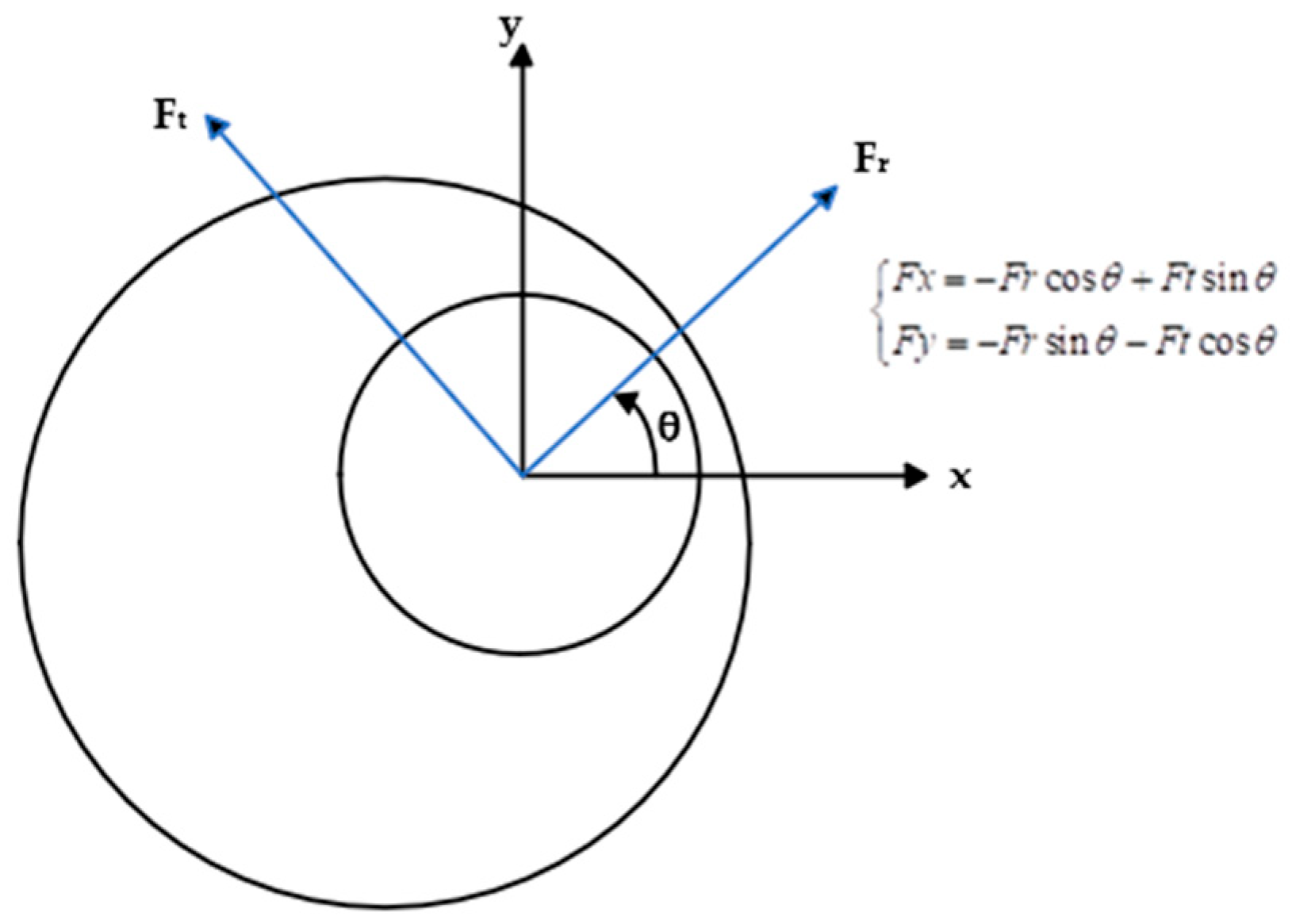
Proceeding with a brief overview of the squeeze film damper (SFD) element, a schematic of the SFD oil film force is depicted as follows, with the inner circle representing the shaft journal and the outer circle representing the SFD outer race, and the space between them filled with the oil film. The direction of the oil film force acting on the journal is as illustrated in the expression.

The restoring force exerted on the rotating shaft due to the oil film force is

$$\begin{array}{l}\left\{\begin{array}{l}{F}_x=-F_r\cos \theta +F_t\sin \theta =-F_r{\displaystyle \frac{v}{e}}+F_t{\displaystyle \frac{w}{e}}\\ F_y=-F_r\sin \theta -F_t\cos \theta =-F_r{\displaystyle \frac{w}{e}}-F_t{\displaystyle \frac{v}{e}}\end{array}\right.\\ \left\{\begin{array}{l}v=e\cdot \cos \theta \\ w=e\cdot \sin \theta \end{array}\right.\end{array}$$

(50)

The signs of Fr and Ft are positive when they are in the same direction as the arrows in Figure 1, and negative when they are opposite to the arrow direction. It is important to note that the restoring force is considered positive when its direction is towards the center of the journal bearing.

The eccentricity $\epsilon$ is defined as the ratio $\epsilon =e/C$, where e is the eccentricity distance, and C is the radial clearance of the oil film. The relationship between the journal displacement and the eccentricity e is expressed as

$$\begin{array}{l}\left\{\begin{array}{l}v=e\cdot \cos \theta \\ w=e\cdot \sin \theta \end{array}\right.\\ {\displaystyle \frac{w}{v}}=\tan \theta ,{\displaystyle \frac{\dot{w}v-w\dot{v}}{v^2}}={\displaystyle \frac{1}{{\cos }^2\theta }}\dot{\theta },\\ \dot{\theta }={\displaystyle \frac{\dot{w}v-w\dot{v}}{v^2}}{\cos }^2\theta ={\displaystyle \frac{\dot{w}v-w\dot{v}}{v^2}}{\displaystyle \frac{v^2}{e^2}}={\displaystyle \frac{\dot{w}v-w\dot{v}}{v^2+w^2}}\\ e^2=v^2+w^2\\ \dot{e}={\displaystyle \frac{v\dot{v}+w\dot{w}}{e}}\end{array}$$

(51)

Taking the short bearing as an example and considering the semi-oil film model,

$$\begin{array}{l}\left\{\begin{array}{l}{F}_r=-{\displaystyle \frac{\mu R{L}^3}{C^2}}\left(I_1\dot{\epsilon }+I_2\epsilon \dot{\theta }\right)\\ F_t=-{\displaystyle \frac{\mu R{L}^3}{C^2}}\left(I_2\dot{\epsilon }+I_3\epsilon \dot{\theta }\right)\end{array}\right.\\ I_1={\displaystyle \frac{\pi \left(1+2{\epsilon }^2\right)}{2{\left(1-{\epsilon }^2\right)}^{2.5}}},I_2={\displaystyle \frac{2\epsilon }{{\left(1-{\epsilon }^2\right)}^2}},I_3={\displaystyle \frac{\pi }{2{\left(1-{\epsilon }^2\right)}^{1.5}}}\end{array}$$

(52)

Substituting Equation (52) into (50) yields the restoring force exerted by the SFD oil film force as

$$\left\{\begin{array}{l}{F}_x=-F_r\cos \theta +F_t\sin \theta ={\displaystyle \frac{\mu R{L}^3}{C^2}}\left(I_1\dot{\epsilon }+I_2\epsilon \dot{\theta }\right){\displaystyle \frac{v}{e}}-{\displaystyle \frac{\mu R{L}^3}{C^2}}\left(I_2\dot{\epsilon }+I_3\epsilon \dot{\theta }\right){\displaystyle \frac{w}{e}}\\ F_y=-F_r\sin \theta -F_t\cos \theta ={\displaystyle \frac{\mu R{L}^3}{C^2}}\left(I_1\dot{\epsilon }+I_2\epsilon \dot{\theta }\right){\displaystyle \frac{w}{e}}+{\displaystyle \frac{\mu R{L}^3}{C^2}}\left(I_2\dot{\epsilon }+I_3\epsilon \dot{\theta }\right){\displaystyle \frac{v}{e}}\end{array}\right.$$

(53)

$$\left\{F_{sfd}\right\}={\left\{F_{x_i},F_{x_j}\right\}}^T$$

(54)

2.4. The Support Restoring Force

In addition to the nonlinear oil film force of the squeeze film damper (SFD), another component of nonlinear force must be taken into account, namely, the nonlinear restoring force of the support. Similarly to the SFD oil film force, the support restoring force in this study is also applied to the support element in the form of a load.

The nonlinear restoring force induced by the action of the support is given by

$$\left\{\begin{array}{l}{F}_x=k_{b}v+k_{bnl}{v}^3\\ F_y=k_{b}w+k_{bnl}{w}^3\end{array}\right.$$

(55)

Herein, $k_b$ represents the support stiffness, and $k_{bnl}$ denotes the coefficient of the support’s nonlinear restoring force.

Rewritten in terms of the nodal displacement array of the element, the expression becomes

$$\begin{array}{c}\left\{\begin{array}{l}{F}_{xi}\\ F_{yi}\\ M_{xi}\\ M_{yi}\end{array}\right\}=\left[\begin{array}{cccc}{k}_{11}^b& 0& 0& 0\\ 0& k_{22}^b& 0& 0\\ 0& 0& 0& 0\\ 0& 0& 0& 0\end{array}\right]\left\{\begin{array}{l}{v}_i\\ w_i\\ {v^{\prime }}_i\\ {w^{\prime }}_i\end{array}\right\}=\left\{K_b^e\right\}\left\{{\delta }^e\right\}\\ k_{11}^b=k_{22}^b=k_b\hfill \end{array}$$

(56)

The nonlinear component, expressed in the form of force, is given by

$$\begin{array}{l}\left\{\begin{array}{l}{F}_{bnl{x}_i}=k_{bnl}{v}^3\\ F_{bnl{x}_j}=k_{bnl}{w}^3\end{array}\right.\\ \left\{F_{bnl}\right\}={\left\{F_{bnl{x}_i},F_{bnl{x}_j}\right\}}^T\end{array}$$

(57)

2.5. Assembly of the Global Matrices

By integrating the preceding equations, we can establish a novel finite element model in which both nonlinear forces are represented as external forces. This approach enables an intuitive analysis of how these nonlinear forces influence the rotor’s response. In summary, building upon the free vibration governing equations of the Euler–Bernoulli beam and incorporating the squeeze film damper (SFD) oil film restoring force, lumped mass elements, and nonlinear support forces, the global matrix is derived by assembling the aforementioned matrices according to the degree of freedom (DOF) ordering, as follows:

$$\begin{array}{l}M\ddot{\delta }+G\dot{\delta }+K\delta =F_{sfd}+F_{bnl}\\ \left\{M\right\}={\displaystyle \sum \left\{M^e\right\}}+{\displaystyle \sum \left\{M_{lump}^e\right\}}\\ \left\{G\right\}={\displaystyle \sum \left\{G^e\right\}}+{\displaystyle \sum \left\{G_{lump}^e\right\}}\\ \left\{K\right\}={\displaystyle \sum \left\{K^e\right\}}+{\displaystyle \sum \left\{K_b^e\right\}}\end{array}$$

(58)

$$\begin{array}{l}{F}_{sfd}={\left[F_x,F_y\right]}^T\\ =\left\{\begin{array}{l}{F}_x=-F_r\cos \theta +F_t\sin \theta ={\displaystyle \frac{\mu R{L}^3}{C^2}}\left(I_1\dot{\epsilon }+I_2\epsilon \dot{\theta }\right){\displaystyle \frac{v}{e}}-{\displaystyle \frac{\mu R{L}^3}{C^2}}\left(I_2\dot{\epsilon }+I_3\epsilon \dot{\theta }\right){\displaystyle \frac{w}{e}}\\ F_y=-F_r\sin \theta -F_t\cos \theta ={\displaystyle \frac{\mu R{L}^3}{C^2}}\left(I_1\dot{\epsilon }+I_2\epsilon \dot{\theta }\right){\displaystyle \frac{w}{e}}+{\displaystyle \frac{\mu R{L}^3}{C^2}}\left(I_2\dot{\epsilon }+I_3\epsilon \dot{\theta }\right){\displaystyle \frac{v}{e}}\end{array}\right.\end{array}$$

(59)

$$\begin{array}{l}\left\{F_{bnl}\right\}={\left\{F_{bnl{x}_i},F_{bnl{x}_j}\right\}}^T\\ =\left\{\begin{array}{l}{F}_{bnl{x}_i}=k_{bnl}{v}^3\\ F_{bnl{x}_j}=k_{bnl}{w}^3\end{array}\right.\end{array}$$

(60)

In this context, M, G, and K represent the global mass matrix, the overall gyroscopic matrix, and the global stiffness matrix (which includes the linear component of the support force, excluding the SFD force), respectively; F_sfd denotes the load array for the oil film force; and F_bnl signifies the nonlinear component of the support force.

3. Calculation of Critical Speeds

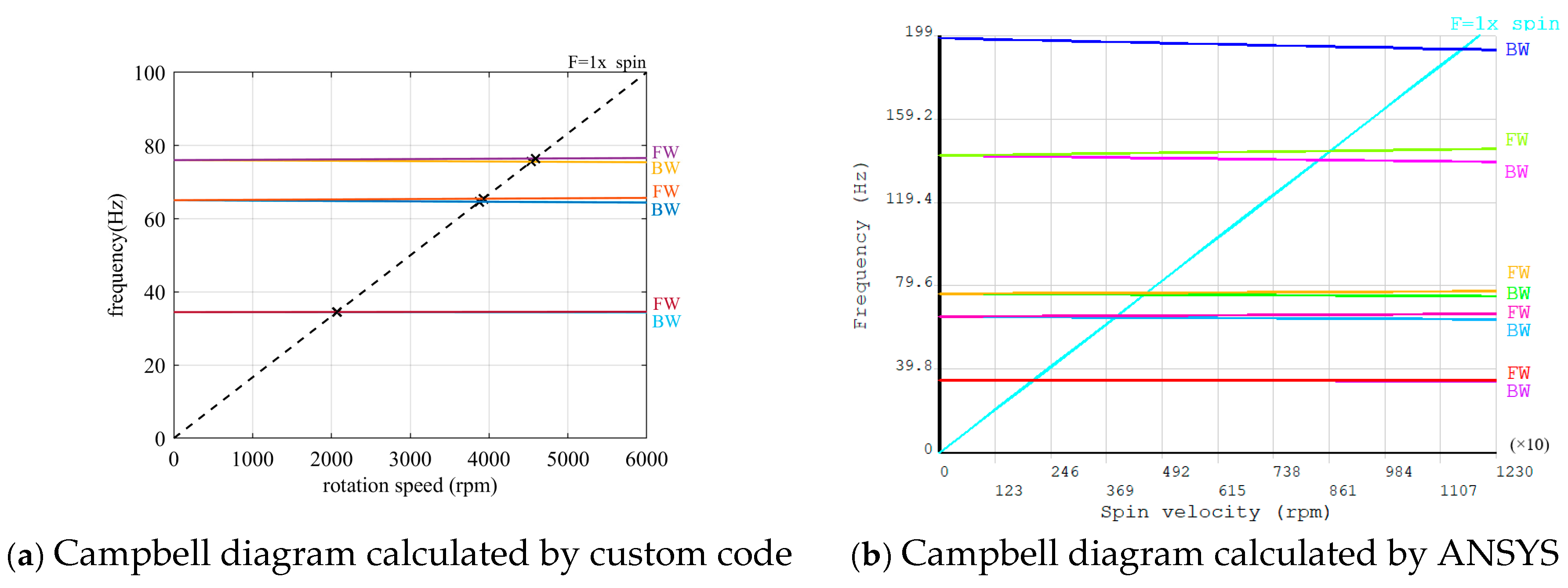
Based on the global motion equation established in the preceding context, without considering the SFD oil film force and the nonlinear restoring force of the supports, the beam model was solved using both custom-coded software and ANSYS 2023 R1. The resulting Campbell diagram and critical speeds were obtained and compared to verify the correctness and accuracy of the code. As depicted in Figure 2, the overall model comprises the Euler–Bernoulli beam model, eight concentrated masses, and three supports. Furthermore, the concentrated masses represent the six-stage compressor and two-stage turbine.

As shown in Equation (58), the global stiffness matrix, mass matrix, and gyroscopic matrix of the model were assembled according to the nodal degree of freedom ordering, and the finite element code written was then utilized to solve the model.

The subsequent calculations of the Campbell diagram were performed using both custom code and ANSYS. The first three critical speeds were then extracted from the diagram for comparison.

As shown in the Campbell diagram (Figure 3) and

Table 1. Comparison of critical speeds for a beam.

Order Number	Critical Speed from Custom Code Solution (rpm)	Critical Speed from ANSYS Solution (rpm)	Difference (%)
First Order	2071.14 (34.52 Hz)	2077.8 (34.63 Hz)	0.32
Second Order	3929.41 (65.50 Hz)	3973.8 (66.23 Hz)	1.11
Third Order	4587.68 (76.46 Hz)	4621.2 (77.02 Hz)	0.72

, the first three critical speeds calculated by the self-developed code and ANSYS for a beam length of 2 m differ by less than 2%, demonstrating the correctness and accuracy of the established model.

In Figure 3, FW denotes forward rotation, BW denotes backward rotation, and F=1×spin represents a line indicating one-fold constant rotational speed.

4. Solution of Equations Using the Newmark β Method

Due to the significant impact of nonlinearity in the study of SFD on rotor response, the Newmark method was employed to solve the control equations established previously, which include the SFD oil film force and the nonlinear restoring force of the supports.

After discretizing the Euler–Bernoulli beam vibration equation using the finite element method and similar approaches, the vibration equation takes the following form:

$$M\ddot{u}\left(t\right)+C\dot{u}\left(t\right)+f\left(t\right)=F\left(t\right)$$

(61)

It is commonly assumed that the mass matrix M and the damping matrix C are constant, while f(t) represents the nonlinear restoring force. At time $t+\Delta t$, the dynamic equilibrium equation must also be satisfied:

$$M\ddot{u}\left(t+\Delta t\right)+C\dot{u}\left(t+\Delta t\right)+f\left(t+\Delta t\right)=F\left(t+\Delta t\right)$$

(62)

Expanding the restoring force $f\left(t+\Delta t\right)$ in a Taylor series around time t, and neglecting higher-order terms, yields

$$f\left(t+\Delta t\right)\dot{=}f\left(t\right)+K\left(t\right)\Delta u$$

(63)

where K(t) is the tangent stiffness matrix at time t. It can be observed that Equation (63) utilizes the tangent stiffness matrix at time t, which is an approximation; hence, it introduces an error. To refine the solution, the Newton–Raphson method is employed for iteration, progressively converging towards the true solution. Substituting Equation (63) into (62) results in

$$M\ddot{u}\left(t+\Delta t\right)+C\dot{u}\left(t+\Delta t\right)+K\left(t\right)\Delta u=F\left(t+\Delta t\right)-f\left(t\right)$$

(64)

In Equation (64), there are 3n unknowns $\ddot{u}\left(t+\Delta t\right)$, $\dot{u}\left(t+\Delta t\right)$ and $\Delta u$, yet there are only three equations, necessitating the addition of 2n constraint conditions. The Newmark Beta method is proposed to construct these constraint conditions, which will be elaborated later. Once the constraint conditions are incorporated, $\ddot{u}\left(t+\Delta t\right)$, $\dot{u}\left(t+\Delta t\right)$ and $\Delta u$ can be determined, thus providing an approximate value for the displacement at time $t+\Delta t$.

$$u\left(t+\Delta t\right)=u\left(t\right)+\Delta u$$

(65)

Assuming that a precise solution has been obtained at time t, the iterative process at time $t+\Delta t$ in accordance with the Newton–Raphson method adopts the state at time t as the initial condition, that is,

$$\begin{array}{l}{u}^{\left(0\right)}\left(t+\Delta t\right)=u\left(t\right)\\ f^{\left(0\right)}\left(t+\Delta t\right)=f\left(t\right)\\ K^{\left(0\right)}\left(t\right)=K\left(t\right)\end{array}$$

(66)

For the k = 1, 2, … iteration steps, it follows that

$$M{\ddot{u}}^{\left(k\right)}\left(t+\Delta t\right)+C{\dot{u}}^{\left(k\right)}\left(t+\Delta t\right)+K^{\left(k-1\right)}\Delta u^{\left(k\right)}=F\left(t+\Delta t\right)+f^{\left(k-1\right)}\left(t+\Delta t\right)$$

(67)

$$u^{\left(k\right)}\left(t+\Delta t\right)=u^{\left(k-1\right)}\left(t+\Delta t\right)+\Delta u^{\left(k\right)}$$

(68)

During the first iteration step k = 1, Equations (67) and (68) simplify to Equations (64) and (65), respectively. In subsequent iterations, the most recent estimates of displacement are utilized to recalculate the restoring force $f^{\left(k-1\right)}\left(t+\Delta t\right)$ and the tangent stiffness $K\left(t\right)$. If the balance in Equation (62) is not achieved, an increment in displacement is required, continuing until equilibrium in Equation (62) is reached.

Due to the high computational cost of regenerating the tangent stiffness $K^{\left(k-1\right)}$ at each iteration step for large structural systems, the modified Newton–Raphson method can also be employed for iteration. The modified Newton–Raphson method utilizes the tangent stiffness matrix $K\left(t\right)$ from time t throughout the entire iterative solution process at time $t+\Delta t$. At this point, the iteration format (67) is revised to

$$M\ddot{u}\left(t+\Delta t\right)+C{\dot{u}}^{\left(k\right)}\left(t+\Delta t\right)+K\left(t\right)\Delta u^{\left(k\right)}=F\left(t+\Delta t\right)-f^{\left(k-1\right)}\left(t+\Delta t\right)$$

(69)

Proceeding with the construction of constraint conditions using the Newmark Beta method, and based on the Lagrange mean value theorem, the velocity at time $t+\Delta t$ is expressed as

$${\dot{u}}_i={\dot{u}}_{i-1}+{\ddot{u}}^{*}\Delta t$$

(70)

The subscript $i-1$ denotes the physical quantity at time t, while the subscript i denotes the physical quantity at time $t+\Delta t$. ${\ddot{u}}^{*}$ represents the acceleration vector $\ddot{u}$ at some point within the interval $\left(t,t+\Delta t\right)$. The Newmark Beta method makes an approximate assumption given by

$${\dot{u}}_i=\left(1-\delta \right){\ddot{u}}_{i-1}+\delta {\ddot{u}}_i$$

(71)

Thus, the velocity at time $t+\Delta t$ can be expressed as

$${\dot{u}}_i={\dot{u}}_{i-1}+\left(1-\delta \right){\ddot{u}}_{i-1}\Delta t+\delta {\ddot{u}}_i\Delta t$$

(72)

Derived from the Taylor series expansion, we have

$$u_i=u_{i-1}+{\dot{u}}_{i-1}\Delta t+\left[\left({\displaystyle \frac{1}{2}}-\beta \right){\ddot{u}}_{i-1}+\beta {\ddot{u}}_i\right]\Delta t^2$$

(73)

In Equations (72) and (73), the parameters $\delta$ and $\beta$ are related to the accuracy and stability of the method. When $\delta >1/2$, algorithmic damping is introduced, leading to perceived amplitude decay; when $\delta <1/2$, negative damping occurs, causing the amplitude to grow during the integration process. Typically, the critical value $\delta =1/2$ is chosen. With $\delta =1/2$, setting $\beta =0$ corresponds to the constant acceleration method, also known as the central difference method; $\beta =1/4$ corresponds to the average acceleration method; and $\beta =1/6$ corresponds to the linear acceleration method.

Rewriting Equation (67) into expressions for velocity increment and acceleration increment, we obtain

$$\left\{\begin{array}{l}{\dot{u}}_i=a_1\left(u_i-u_{i-1}\right)+\left(1-a_4\right){\dot{u}}_{i-1}-a_5{\ddot{u}}_{i-1}\\ {\ddot{u}}_i=a_0\left(u_i-u_{i-1}\right)-a_2{\dot{u}}_{i-1}-\left(a_3-1\right){\ddot{u}}_{i-1}\end{array}\right.$$

(74)

In the aforementioned equation,

$$\begin{array}{l}{a}_0={\displaystyle \frac{1}{\beta \Delta t^2}},a_1={\displaystyle \frac{\delta }{\beta \Delta t}},a_2={\displaystyle \frac{1}{\beta \Delta t}}\\ a_3={\displaystyle \frac{1}{2\beta }},a_4={\displaystyle \frac{\delta }{\beta }},a_5=-\Delta t\left(1-{\displaystyle \frac{\delta }{2\beta }}\right)\end{array}$$

(75)

Rewritten in an iterative format, it becomes

$$\left\{\begin{array}{l}{{\dot{u}}_i}^{\left(k\right)}=a_1\left({u_i}^{\left(k-1\right)}-u_{i-1}+\Delta u^{\left(k\right)}\right)+\left(1-a_4\right){\dot{u}}_{i-1}-a_5{\ddot{u}}_{i-1}\\ {{\ddot{u}}_i}^{\left(k\right)}=a_0\left({u_i}^{\left(k-1\right)}-u_{i-1}+\Delta u^{\left(k\right)}\right)-a_2{\dot{u}}_{i-1}-\left(a_3-1\right){\ddot{u}}_{i-1}\end{array}\right.$$

(76)

Substituting Equation (76) into (69) and rearranging, we arrive at

$$\tilde{K}\Delta u^{\left(k\right)}=\Delta {\tilde{F}}^{\left(k\right)}$$

(77)

In this equation,

$$\begin{array}{c}\tilde{K}=K\left(t\right)+a_{0}M+a_{1}C\\ \Delta {\tilde{F}}^{\left(k\right)}=F\left(t+\Delta t\right)-f^{\left(k-1\right)}\left(t+\Delta t\right)\\ \hspace{1em}\hspace{1em}\hspace{1em}\hspace{1em}\hspace{1em}\hspace{1em}\hspace{1em}\hspace{1em}\hspace{1em}+M\left[a_0\left(u_{i-1}-u_i^{\left(k-1\right)}\right)+a_2{\dot{u}}_{i-1}+\left(a_3-1\right){\ddot{u}}_{i-1}\right]\\ \hspace{1em}\hspace{1em}\hspace{1em}\hspace{1em}\hspace{1em}\hspace{1em}\hspace{1em}\hspace{1em}\hspace{1em}\hspace{1em}\hspace{1em}+C\left[a_1\left(u_{i-1}-u_i^{\left(k-1\right)}\right)+\left(a_4-1\right){\dot{u}}_{i-1}+a_5{\ddot{u}}_{i-1}\right]\Delta u^{\left(k\right)}\end{array}$$

(78)

Subsequently, the finite element model is solved by assembling the stiffness matrix K, mass matrix M, and gyroscopic matrix C according to Equation (58). Here, K includes only the linear part of the support stiffness, while the nonlinear components encompass the SFD oil film force and the nonlinear restoring force of the supports. These are applied to the supports in the form of loads as shown in Equations (59) and (60).

It should be noted that K, M, and C are all independent of time and are related only to the model’s parameters such as length, radius, and density. When constructing the load vector, time-dependent parameters v and w are substituted into Equations (59) and (60), and then the resulting forces are applied to the corresponding degrees of freedom at the relevant nodes.

In the load array, in addition to the SFD oil film force and the nonlinear restoring force of the supports, an unbalanced excitation must also be applied at the concentrated mass nodes, which takes the following form:

$$\left\{\begin{array}{l}{F}_r=me{\omega }^2\cos \left(\omega t\right)\\ F_t=me{\omega }^2\sin \left(\omega t\right)\end{array}\right.$$

(79)

Upon convergence, the displacement at time t is obtained, and the solution is continued up to the predefined endpoint.

$${\dot{u}}_i={\dot{u}}_{i-1}+{\ddot{u}}^{*}\Delta t$$

(80)

5. Computational Analysis

Subsequently, the Newmark Beta method was employed to determine the response of the model. The model in question is a beam model that is 2 m long, equipped with three supports and eight concentrated masses. Analyses were conducted for four distinct scenarios: without nonlinear terms, with SFD nonlinear oil film force, with support nonlinear restoring force, and with the coupling of both nonlinear forces. The analyses encompass amplitude–frequency response analysis, centerline trajectory analysis, and time-domain response analysis, with particular emphasis on conditions near the critical speeds for the latter two.

Firstly, an examination of the amplitude–frequency characteristics was conducted. As the solution was formulated in the time domain, it was essential to introduce damping to mitigate the effects of spurious frequencies. Consequently, a damping mechanism was selected, that could effectively eliminate these frequencies with minimal impact on the overall results.

Following this, an analysis of the centerline trajectory and time-domain response was carried out, with a particular focus on the vicinity of the first three critical speeds identified from the amplitude–frequency characteristic plot.

The rotor model parameters are as follows: The rotor has a total length of 2 m and consists of a solid shaft with a radius of 0.025 m. With one end of the rotor serving as the origin of the coordinate system, the axial coordinates and stiffness values of the bearings are as follows: the first support has an axial coordinate of 0.02 times the total length of the rotor and a stiffness of 1 × 10⁶ N/m; the second support has an axial coordinate of 0.55 times the total length and a stiffness of 1 × 10⁷ N/m; the third support is located at an axial coordinate of 0.825 times the total length, with a stiffness also of 1 × 10⁷ N/m.

5.1. Response Analysis Without Nonlinear Terms

At the outset, an analysis was conducted for the nonlinear term-free scenario (i.e., setting F_sfd and F_bnl in Equation (58) to zero). The investigation focused on three support positions, primarily examining the frequency response characteristics, shaft centerline trajectory, and time-domain response of the system. Specifically, when analyzing the shaft centerline trajectory and time-domain response, the study concentrated on the vicinity of the rotor critical speeds.

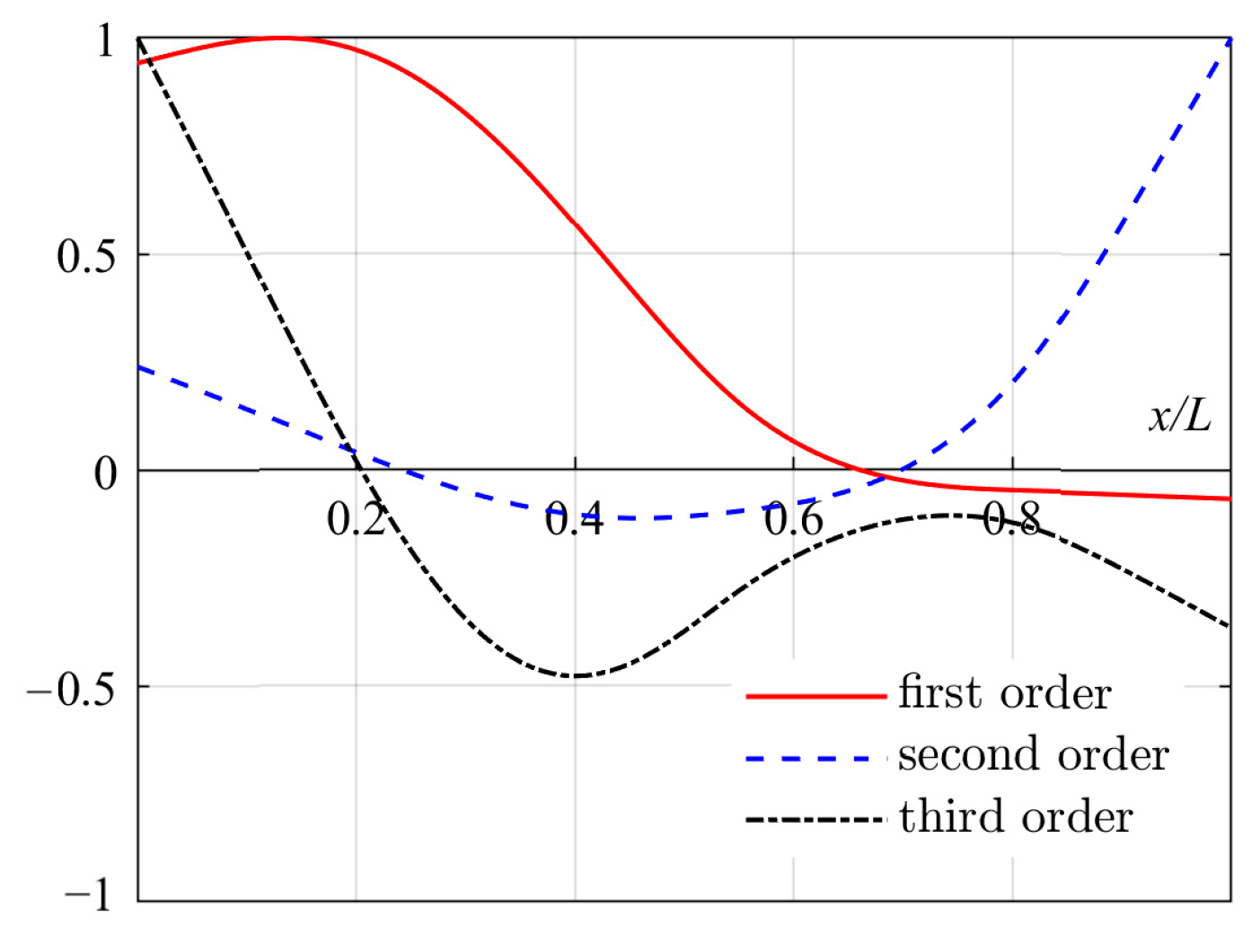
As determined in Section 2, the first three critical speeds of the rotor lie within the range of 2000 to 5000 rpm; hence, this range was selected for solving the amplitude–frequency characteristics. Analysis of the rotor’s modal shape diagram (Figure 4) indicates that applying an unbalanced force at the sixth concentrated mass can excite the third-order critical speed response.

The first three critical speeds of the rotor, as calculated from the Campbell diagram, are presented in Table 1.

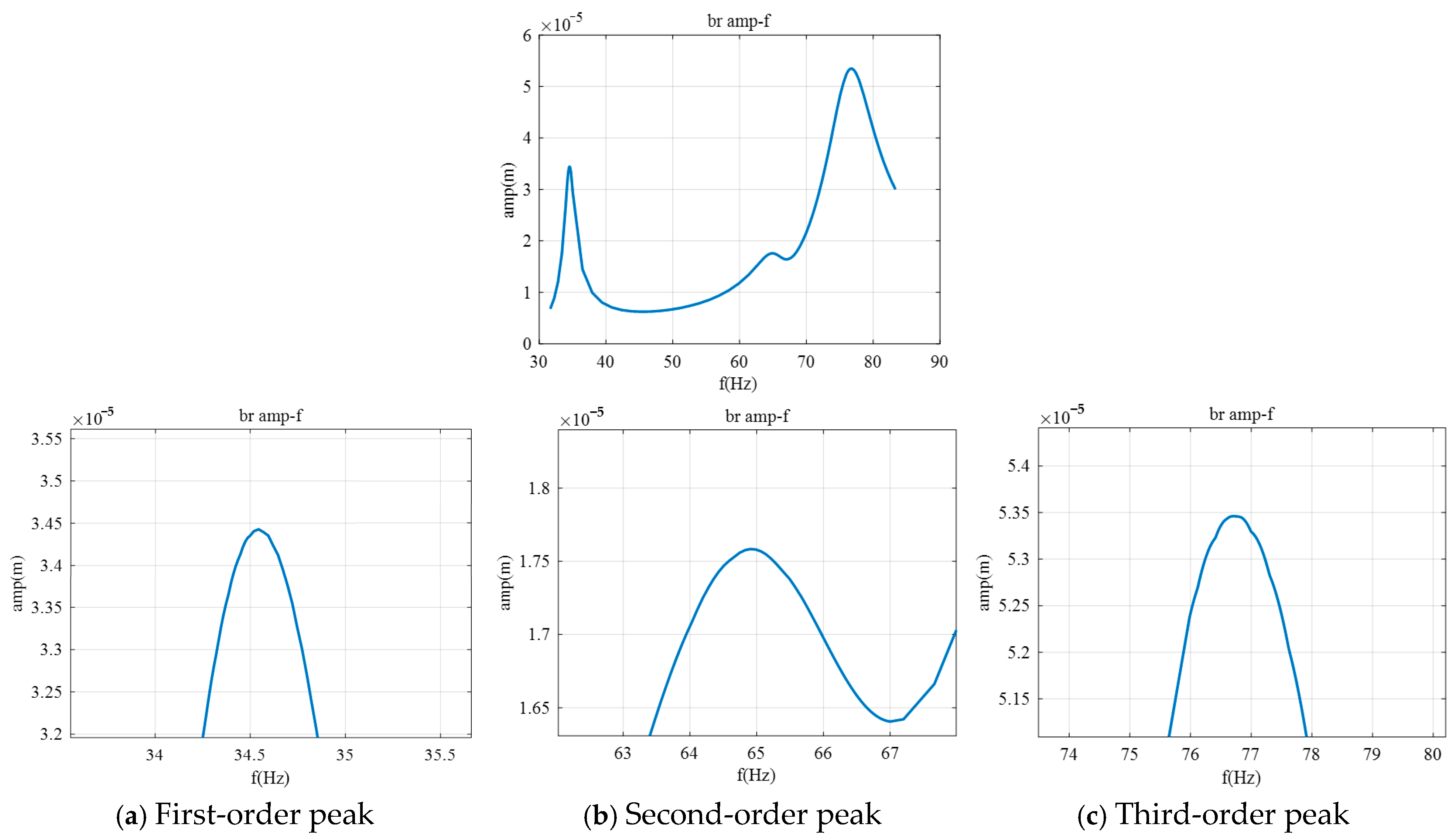
After solving the model over a speed range of 2000 to 5000 rpm using the Newmark Beta method, the resulting amplitude–frequency response is depicted in Figure 5, Figure 6 and Figure 7 below:

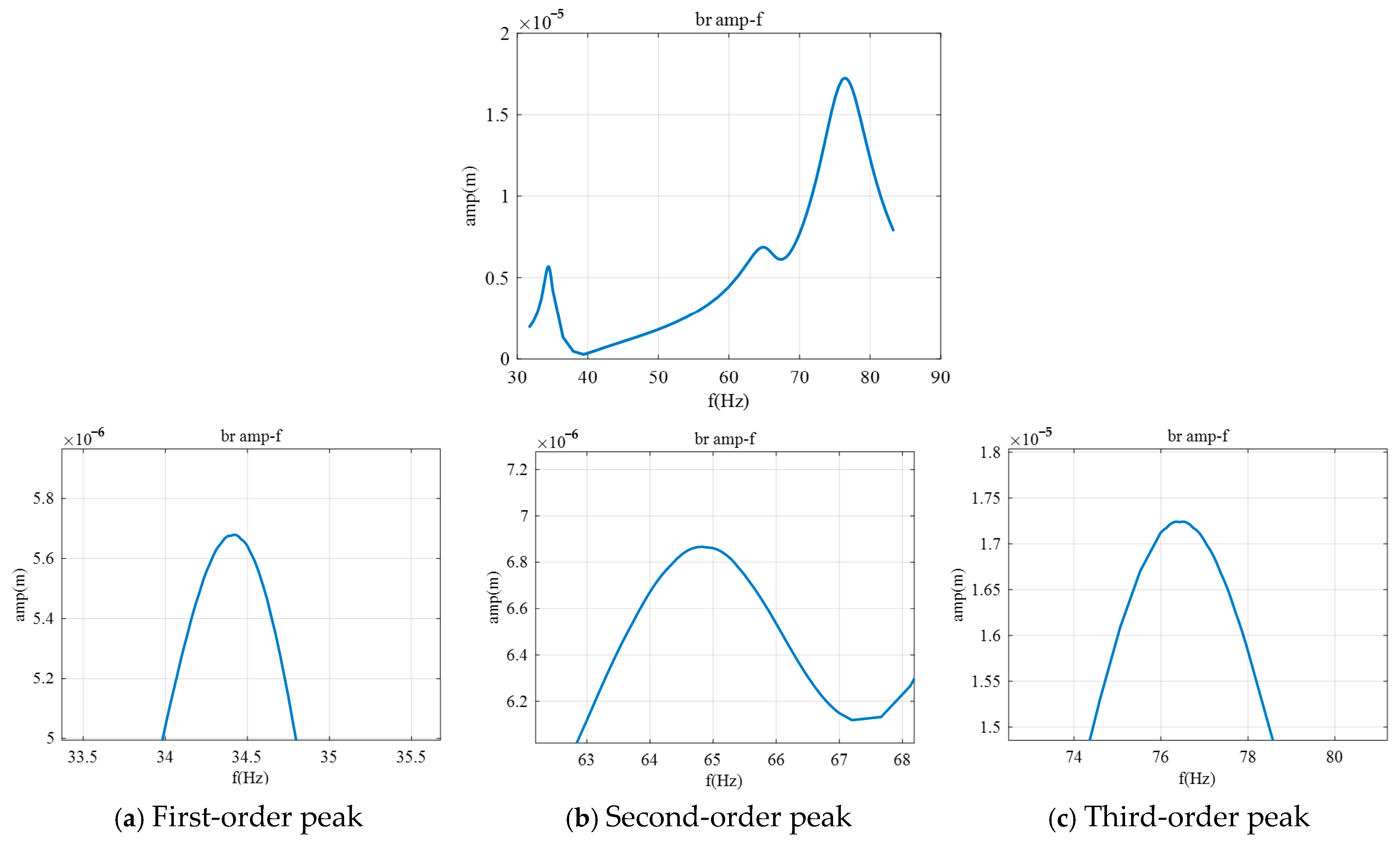
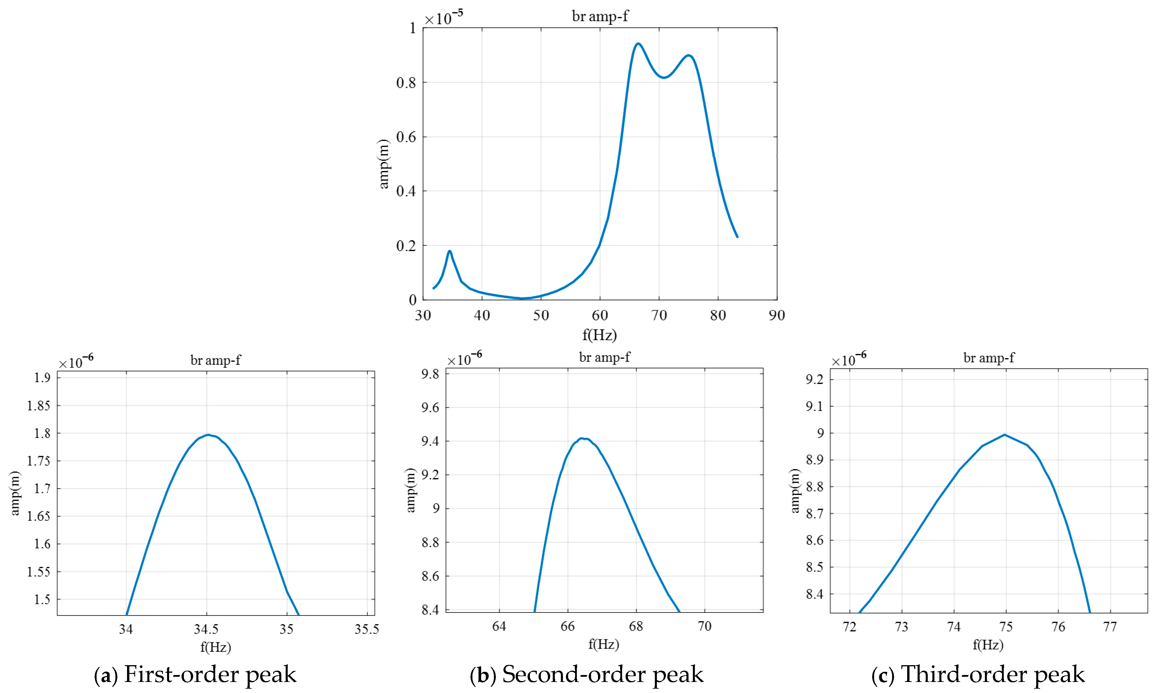
Comparing the amplitude–frequency characteristic graph with the modal shape diagrams reveals that the relative magnitudes of the first to third modal amplitudes at the three bearing positions (0.02, 0.55, 0.852) correspond with their relative sizes in the amplitude–frequency characteristic graph. At the first bearing location, the amplitude of the third critical speed is the highest, the second is the lowest, and the first is slightly lower than the third. At the second bearing location, the amplitude of the third critical speed is the highest, with the second and first being approximately equal, and the second being slightly higher than the first. At the third bearing location, the amplitude of the second critical speed is the highest, with the third and second being approximately equal, and the third being slightly lower than the second, while the first has the lowest amplitude.

5.2. Response Analysis with SFD Nonlinear Oil Film Force

Expanding upon the analysis conducted without considering nonlinear elements, the SFD nonlinear oil film force is integrated into the analysis to assess its impact on the rotor’s amplitude–frequency characteristics, time-domain responses, and orbits at each of the three support locations. Referring to the amplitude–frequency characteristic diagram from the linear scenario, the SFD oil film gap is fine-tuned for each support to ensure that the oil film gap C exceeds the maximum displacement e observed at the rotor’s supports. The formulation for the SFD nonlinear oil film force is depicted in Equation (53).

Adhering to the same rotational speed range of 2000 to 5000 rpm as in the linear case, the amplitude–frequency characteristics are recalculated. An unbalanced force is similarly applied to the sixth concentrated mass. The specific parameters for SFD implementation are detailed in Table 1.

The aforementioned parameters in

Table 2. SFD parameters.

Oil Film Dynamic Viscosity (Pa·s)	Oil Film Radius R (m)	Oil Film Width L (m)
0.02976	0.025	0.005

do not include the oil film gap C. Based on the amplitude–frequency response diagram without nonlinear terms, the oil film gap for the SFD applied at the first support C₁ ranges from 5.45 × 10⁻⁵ m to 6 × 10⁻⁵ m. For the second support, the oil film gap C₂ ranges from 1.6 × 10⁻⁵ m to 1.8 × 10⁻⁵ m, and for the third support, the oil film gap C₃ is 1 × 10⁻⁵ m.

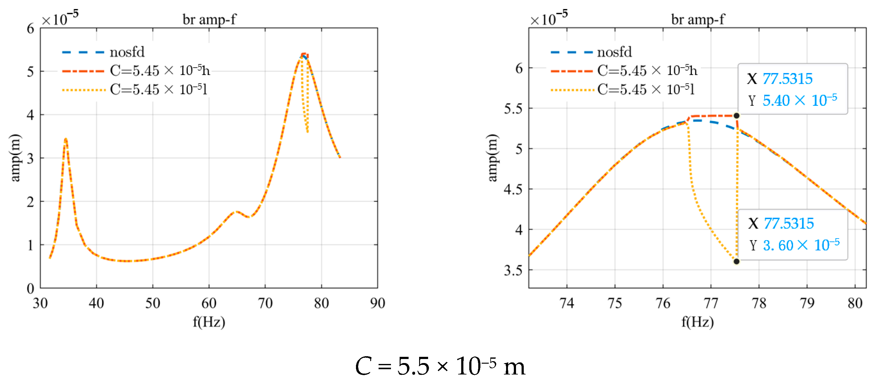
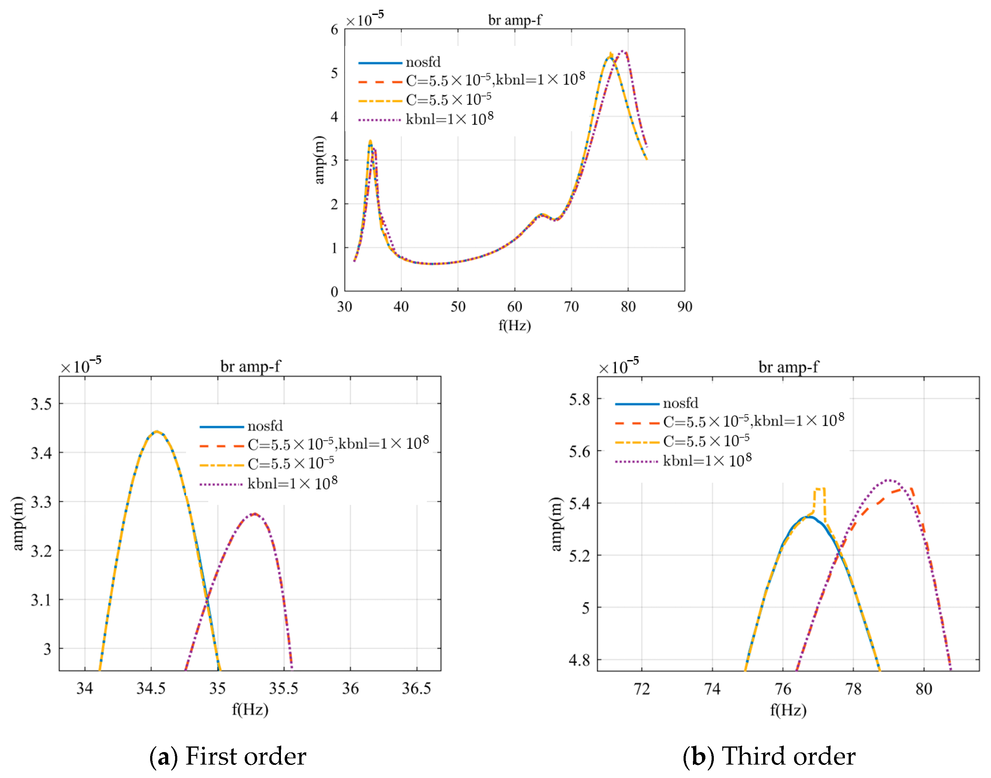
For the first support, calculations were performed based on the scenario without an SFD, assigning an oil film gap C greater than its maximum amplitude value. Within the range of C = 5.45 × 10⁻⁵ m to 5.5 × 10⁻⁵ m, a bi-stable phenomenon was observed, as illustrated in the figure below. As C increased, the bi-stable phenomenon gradually diminished. Further increasing C to 6e−5 m resulted in an insignificant effect from the SFD; hence, the range of C = 5.45 × 10⁻⁵ m to 6 × 10⁻⁵ m was selected for computation. The following figure displays the amplitude–frequency characteristic curve exhibiting the bi-stable phenomenon.

Upon further increasing the oil film gap C, the bi-stable phenomenon has ceased to exist once C reaches 6 × 10⁻⁵ m. Moreover, the SFD exerts a minimal influence on the response and amplitude of the first three critical speeds. When the oil film gap C varies between 5.5 × 10⁻⁵ m and 6 × 10⁻⁵ m, the amplitude changes are less than 0.3%, and the frequency changes are less than 0.5 Hz.

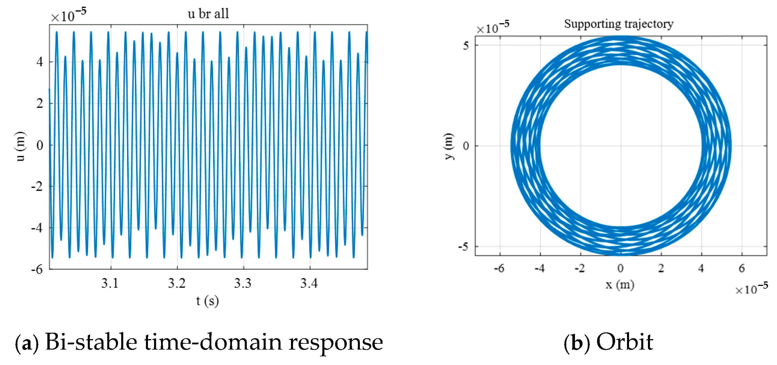
Referring to Figure 8, at the data point where C = 5.5 × 10⁻⁵ m and the frequency is 77.1 Hz, the extracted time-domain response and orbit are illustrated in Figure 9. After the time t exceeds 1 s, the amplitude of the support begins to fluctuate between two values and stabilizes after approximately 3 s, indicative of the bi-stable phenomenon. The orbit of the support is characterized by a circular motion that oscillates between an outer and an inner loop.

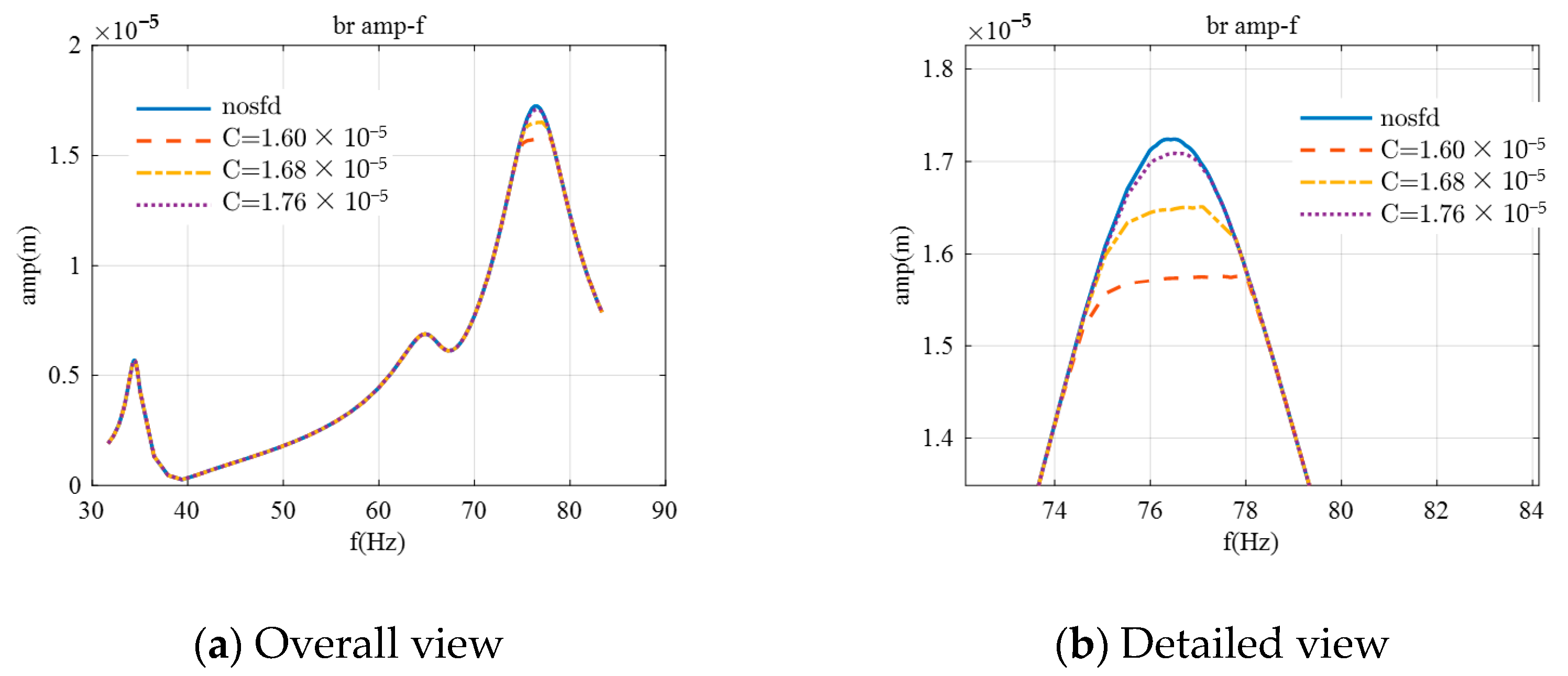
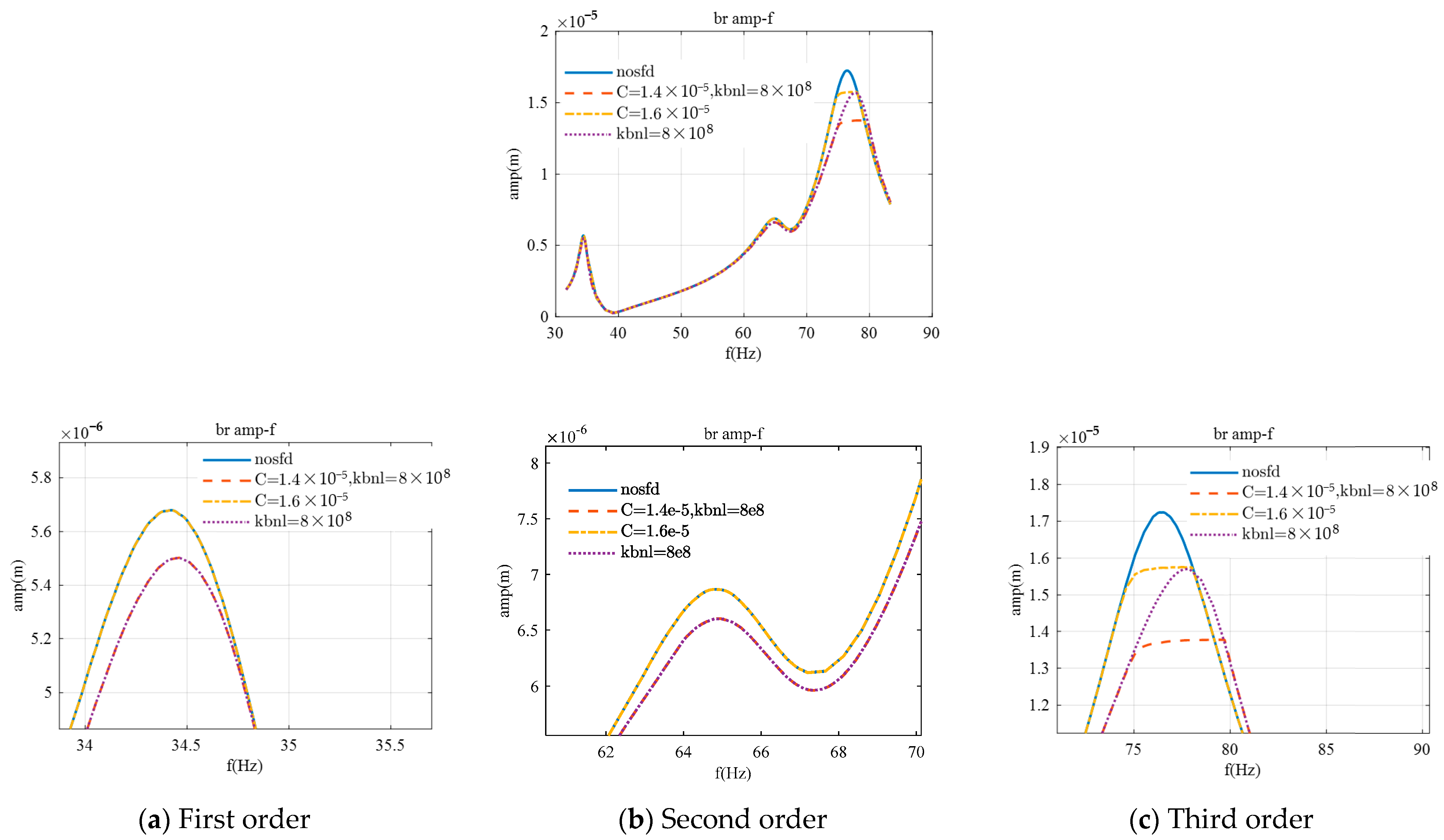
For the second support, calculations were initially performed without an SFD, assigning an oil film gap C larger than its maximum amplitude value. It was observed that the amplitude decreased; however, the effect of the SFD became negligible when the oil film gap exceeded 1.8 × 10⁻⁵ m. Subsequently, calculations were made with a smaller oil film gap C based on the amplitude when C was 1.8 × 10⁻⁵ m. It was found that when the oil film gap C was less than 1.6 × 10⁻⁵ m, the eccentricity distance became greater than the oil film gap, which is not practical. Therefore, the range for the SFD oil film gap C₂ was set between 1.6 × 10⁻⁵ m and 1.8 × 10⁻⁵ m. As shown in the figure below, as the oil film gap C increases, the SFD’s restrictive effect on the amplitude diminishes. Compared to the scenario without an SFD, when C is 1.6 × 10⁻⁵ m, the amplitude is reduced by 8.2%, and when C is greater than 1.8 × 10⁻⁵ m, the amplitude change is less than 1%.

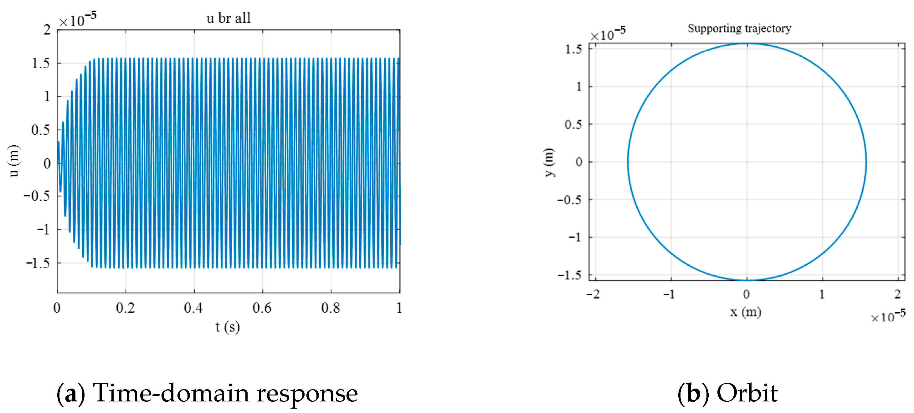
Referring to Figure 10, at the data point where C = 1.6 × 10⁻⁵ m and the frequency is 76.5 Hz, the time-domain response and orbit are extracted. As shown in Figure 11, after the time t exceeds 0.1 s, the amplitude of the support stabilizes. The orbit of the support is characterized by a circular trajectory.

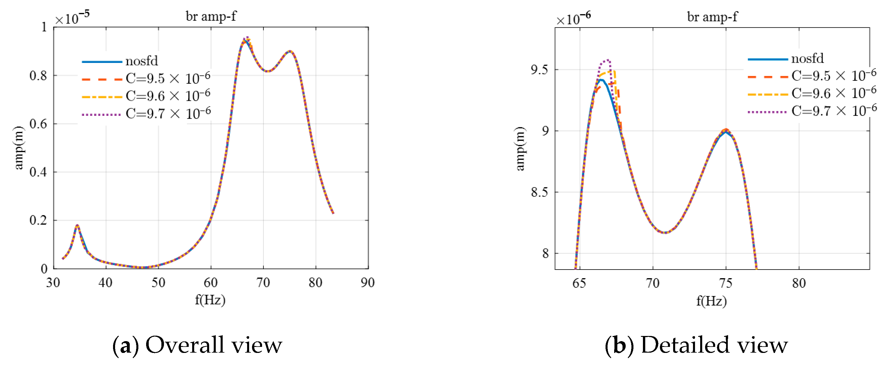
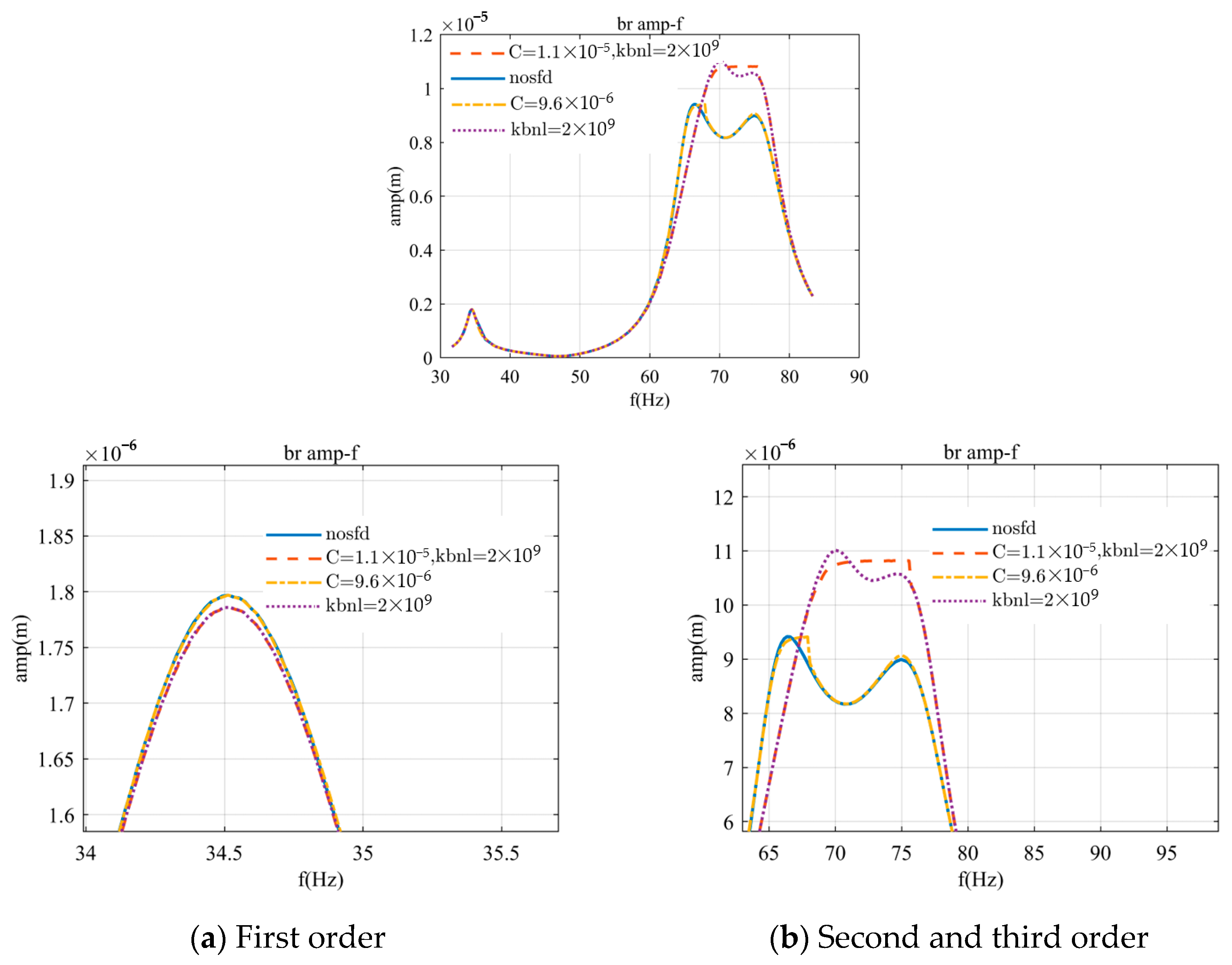
For the third support, employing the same method as described above, the solution range is selected to be C = 9.5 × 10⁻⁶ m to 1 × 10⁻⁵ m. When the oil film width L is 0.005 m, it is not feasible to solve for cases where C is less than 9.8 × 10⁻⁶ m; hence, the oil film width L is reduced to 0.003 m. When the SFD is applied to the third support, the second-order critical speeds are all increased, but the amplitude changes vary. At C = 9.5 × 10⁻⁶ m, the SFD effect is most optimal, with the critical speed increasing by approximately 1 Hz and the amplitude decreasing by 0.6%. As the oil film gap C increases, the increase in critical speed diminishes, and the amplitude actually rises, which is a situation to be avoided in the design of the SFD.

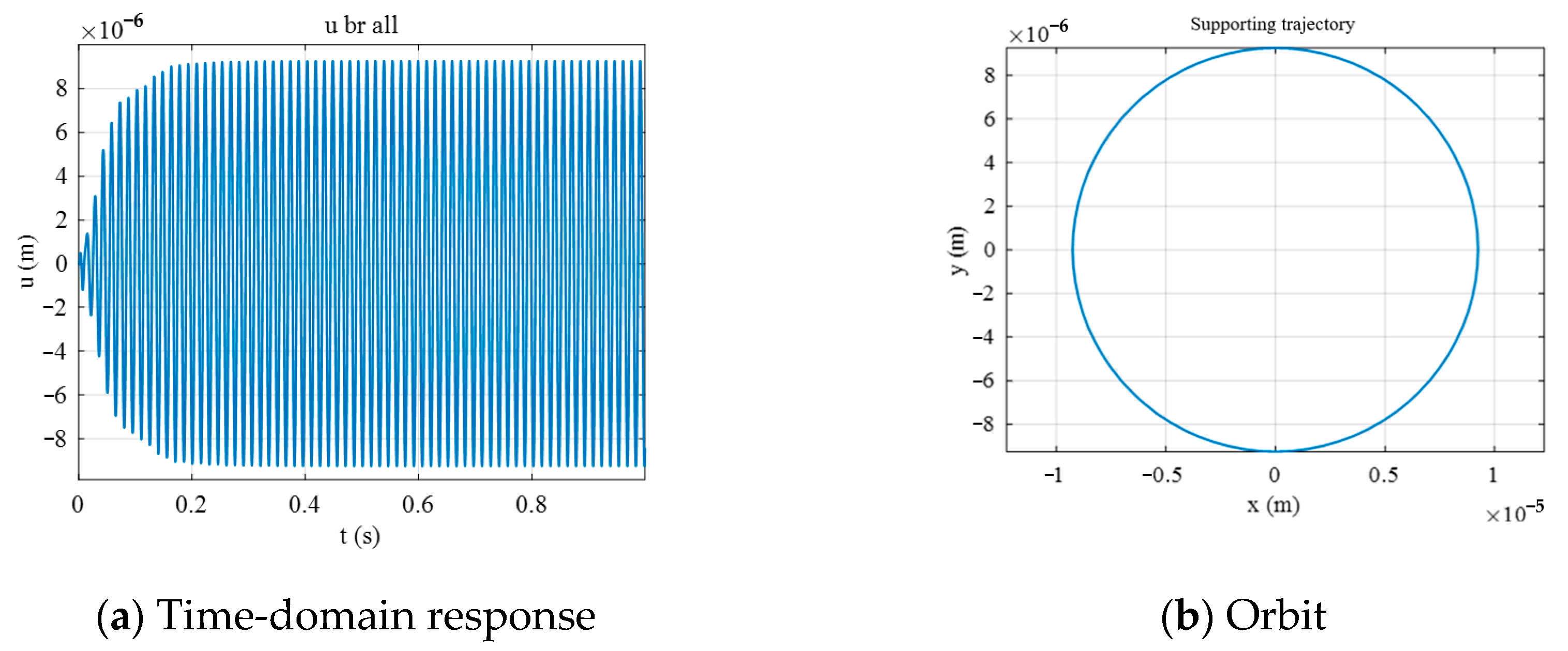
Referring to Figure 12, at the data point where C = 9.5 × 10⁻⁶ m and the frequency is 66.4 Hz, the time-domain response and orbit are extracted. As shown in Figure 13, after the time t exceeds 0.2 s, the amplitude of the support stabilizes. The orbit of the support manifests as a circular trajectory.

Below is a summary of our findings thus far:

• Under ideal conditions, the addition of an SFD at the support can serve to reduce amplitude and increase critical speeds. However, improper design of SFD parameters may not only fail to reduce the amplitude but could also lead to an increase in amplitude and even induce a bi-stable phenomenon, thereby enhancing the overall vibration and destabilizing the rotor’s operating state.
• After the addition of an SFD to the first support, a bi-stable phenomenon occurred near the third critical speed. It was observed that as the oil film gap C increased, which corresponds to a decrease in eccentricity, the bi-stable phenomenon gradually diminished until it disappeared. Thus, a bi-stable phenomenon is likely to occur when the length-to-diameter ratio is 0.2 and the eccentricity is greater than 0.95, and it ceases as the eccentricity decreases.
• Following the addition of an SFD to the second support, the amplitude was somewhat reduced. As the SFD oil film gap C increased, which implies a decrease in eccentricity, the change in amplitude became less pronounced. Compared to the scenario without an SFD, when C exceeds 1.8 × 10⁻⁵ m, the amplitude variation is less than 1%.
• After the addition of an SFD to the third support, the amplitude near the second critical speed was somewhat reduced, and the critical speed itself increased. When the length-to-diameter ratio is 0.12 and the eccentricity is 0.99, the amplitude decreased.

5.3. Response Analysis with Support Nonlinear Restoring Force

Building upon the analysis without nonlinear terms, the analysis now incorporates the support nonlinear force to examine its impact on the rotor’s amplitude–frequency characteristics, time-domain response, and orbit at the three supports. The form of the SFD nonlinear oil film force is as indicated in Equation (55).

An unbalanced force is also applied at the sixth concentrated mass. The influence of the support nonlinear restoring force on the amplitude–frequency characteristics at the supports and at the concentrated mass where the unbalance is applied is investigated after imposing the nonlinear restoring force at each of the three supports.

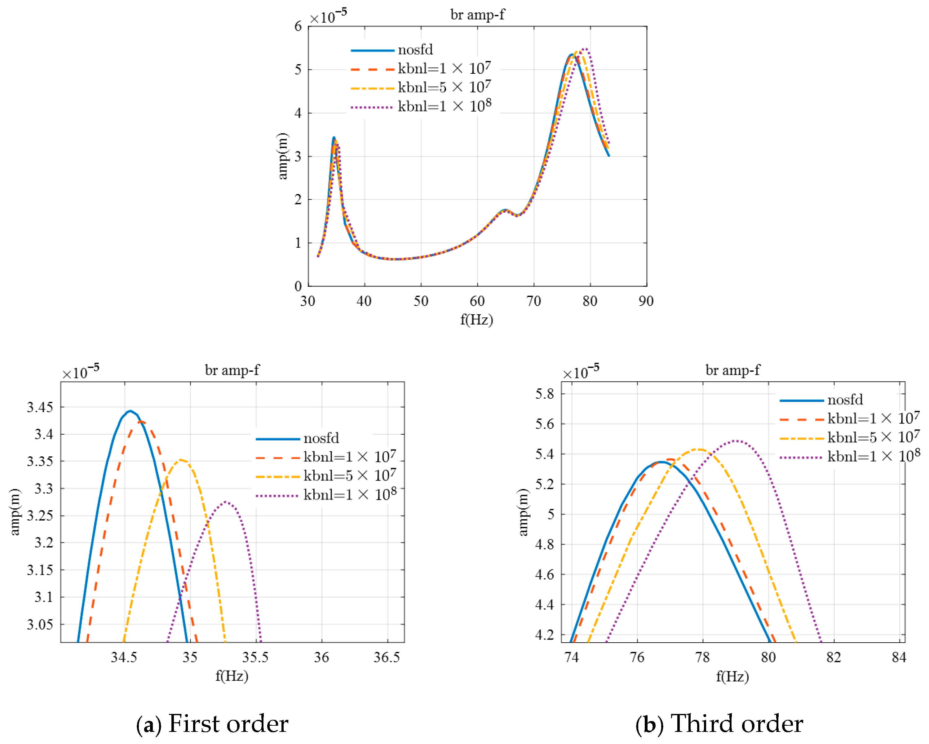
Starting with the first support, based on equivalent stiffness calculations, the restoring force coefficient k_bnl becomes significantly pronounced at 1 × 10⁸. A comparison is made between the results with the restoring force coefficient ranging from 0 to 1e8 to assess the impact of the support restoring force on the rotor’s response. As the coefficient of the support nonlinear force increases, both the amplitude and frequency at the support are affected.

As shown in Figure 14, at the first critical speed near the support, the amplitude decreases while the critical speed increases. With k_bnl at 1 × 10⁸, the amplitude is reduced by 6%, and the critical speed is raised by 0.8 Hz. Conversely, at the third critical speed near the support, the amplitude increases while the critical speed also increases. With k_bnl at 1e8, the amplitude increases by 4%, and the critical speed is elevated by 2.5 Hz.

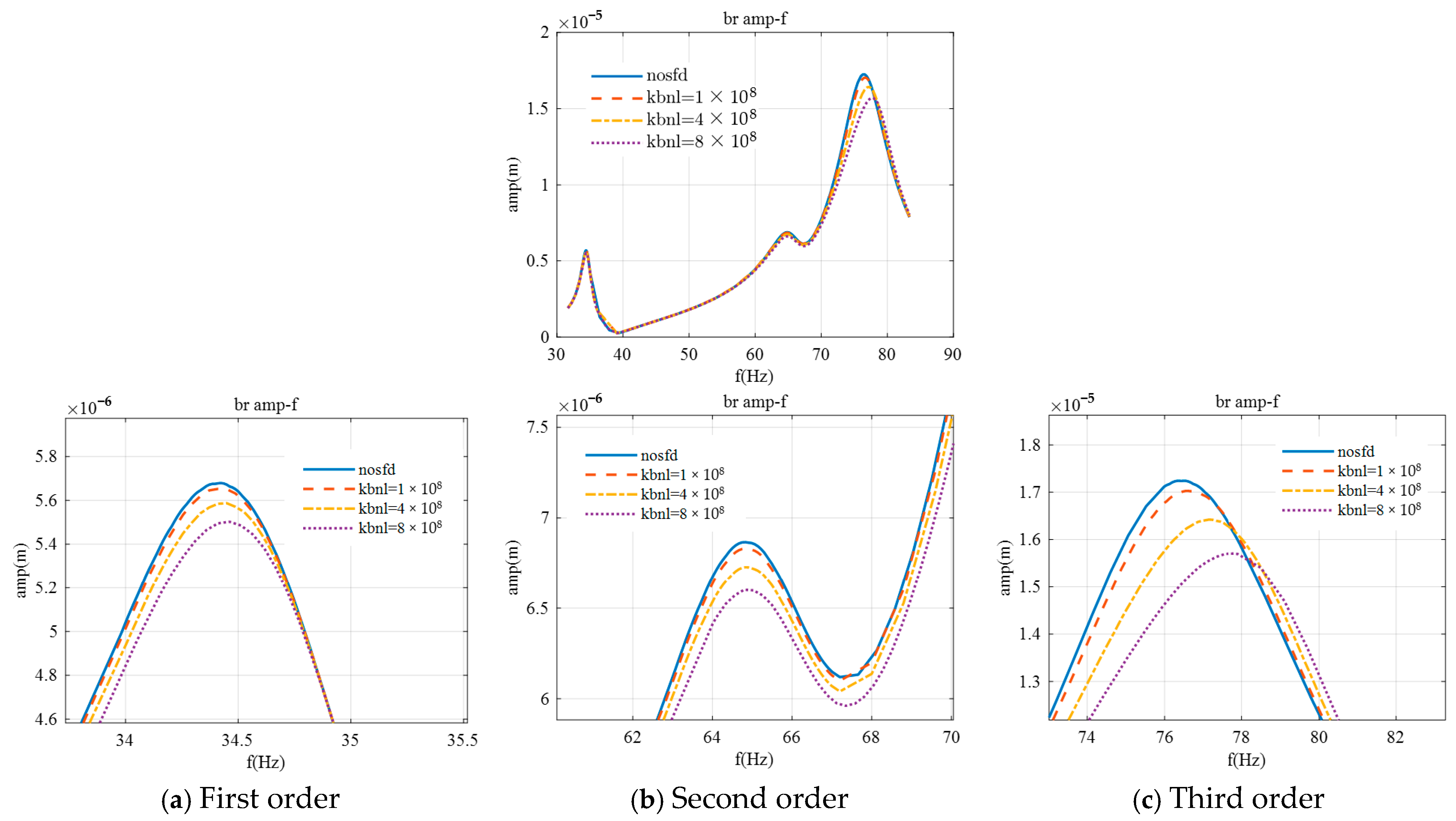
Subsequently, a nonlinear restoring force was added to the second support to observe its impact on the rotor’s response. Based on equivalent stiffness calculations, the range of the restoring force coefficient k_bnl was set from 1 × 10⁸ to 8 × 10⁸.

As shown in Figure 15, with the restoring force coefficient increased, the amplitudes near the first three critical speeds all decreased, and the critical speeds also rose. When the restoring force coefficient k_bnl was 8 × 10⁸, the amplitude near the first critical speed dropped by 3%, and the critical speed increased by 0.5 Hz; the amplitude near the second critical speed decreased by 4%, with no change in the critical speed; and the amplitude near the third critical speed fell by 11%, with the critical speed rising by 1.4 Hz.

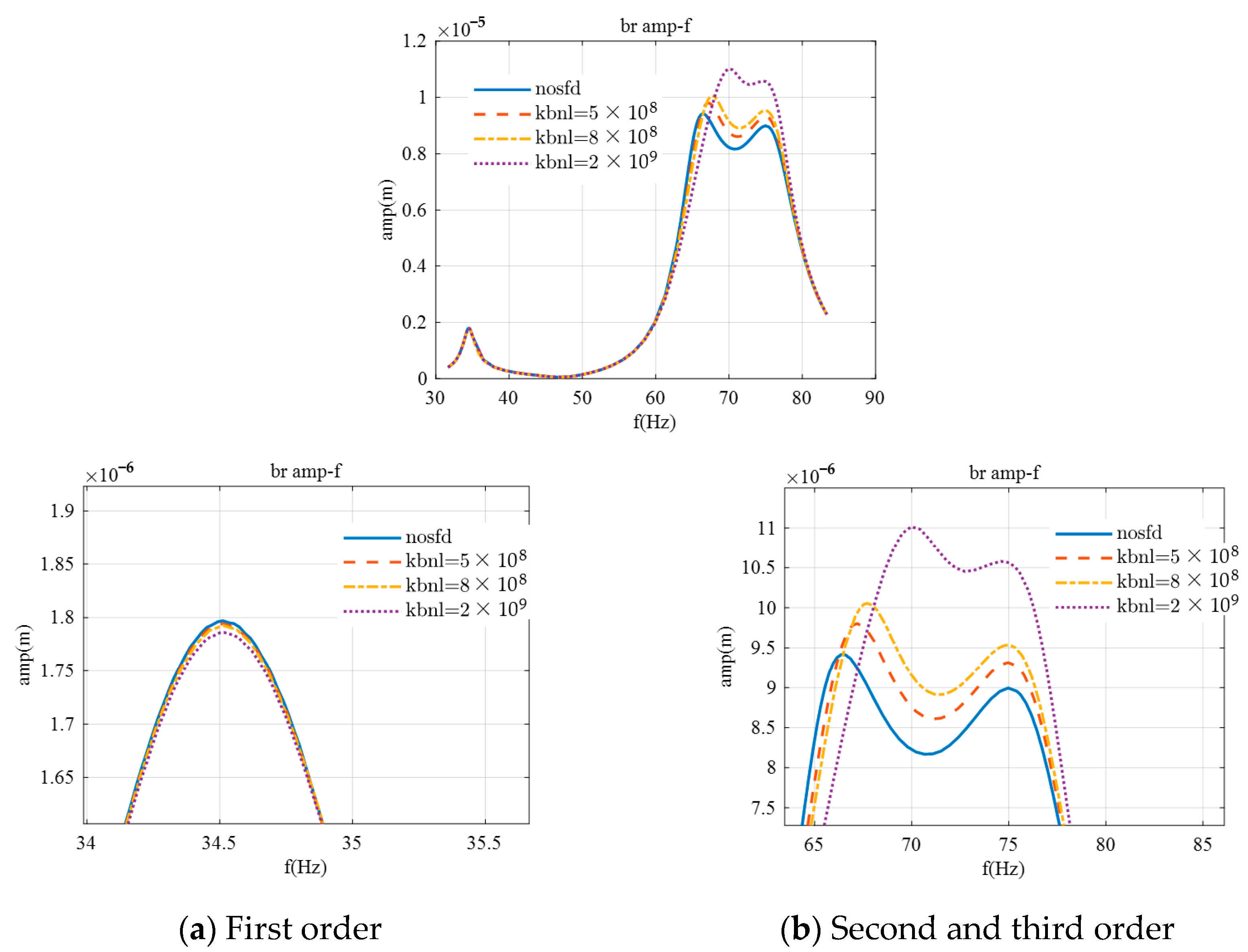
Finally, a nonlinear restoring force was introduced to the third support to observe its impact on the rotor’s response, with the result shown in Figure 16. Based on equivalent stiffness calculations, the range for the restoring force coefficient k_bnl was set between 5 × 10⁸ and 2 × 10⁹. As the restoring force coefficient increased, the amplitude near the first critical speed decreased, with no change in the critical speed. However, the amplitudes near the second and third critical speeds increased, with a rise in the second critical speed.

When the restoring force coefficient k_bnl is set to 2 × 10⁹, the amplitude change near the first critical speed is minimal, decreasing by 0.5%, with no variation in the critical speed. Near the second critical speed, the amplitude increases by 17%, and the critical speed rises by 3.5 Hz. Near the third critical speed, the amplitude increases by 11%, while the critical speed remains unchanged.

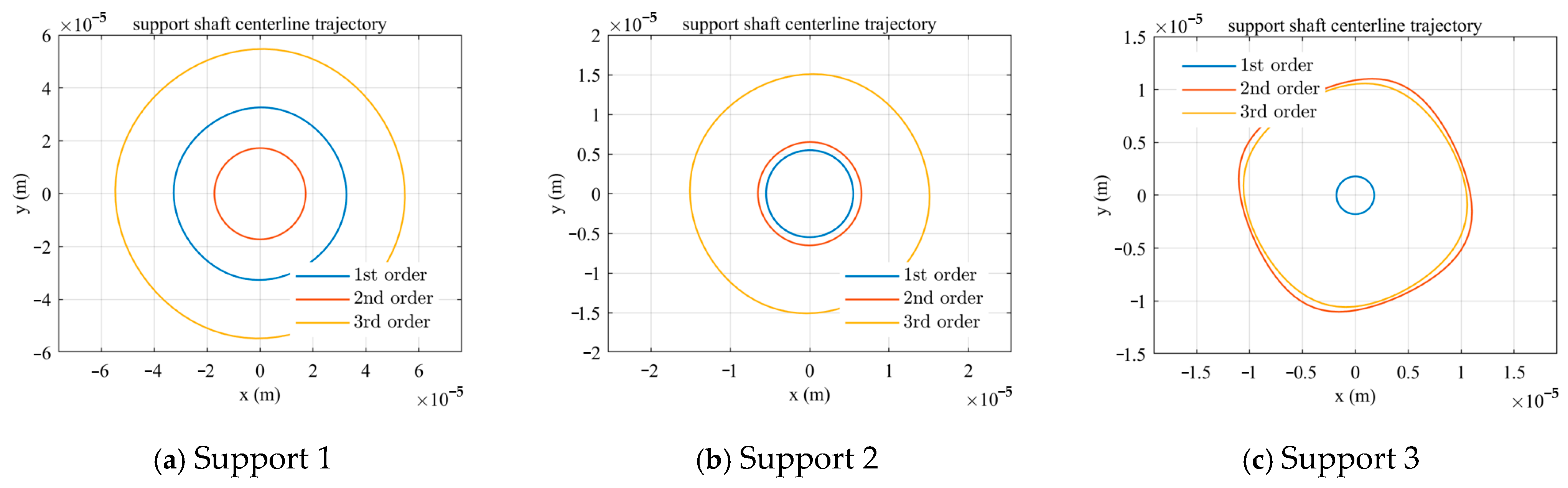
In addition, nonlinear support restoring forces with coefficients k_bnl = 1 × 10⁸, k_bnl = 8 × 10⁸, and k_bnl = 2 × 10⁹ were applied to the three supports, respectively. The centerline trajectories of the shafts under these conditions are shown in Figure 17. It can be observed that the first and second supports maintain circular centerline trajectories even after applying the nonlinear restoring forces. However, for the third support, the centerline trajectory becomes irregular near the second-order and third-order critical speeds when the nonlinear force is introduced.

5.4. Response Analysis with SFD Nonlinear Oil Film Force and Support Nonlinear Restoring Force

Building upon the analysis without nonlinear terms, the analysis now incorporates both the SFD nonlinear oil film force and the support nonlinear restoring force to examine their effects on the rotor’s amplitude–frequency characteristics, time-domain response, and orbit at the three supports. The forms of the SFD nonlinear oil film force and the support nonlinear force are as indicated in Equations (53) and (55), respectively.

Consistent with the scenario without the application of nonlinear forces, the amplitude–frequency characteristics are calculated within the 2000 to 5000 rpm range. An unbalanced force is similarly applied at the sixth concentrated mass. The influence of the support nonlinear restoring force on the amplitude–frequency characteristics at the supports and at the concentrated mass where the unbalance is applied is investigated after imposing the nonlinear forces at each of the three supports.

Starting with the first support, based on the conclusions from the previous sections, the parameters C = 5.52 × 10⁻⁵ m and k_bnl = 1 × 10⁸ are selected to assess the impact of the support restoring force on the rotor’s response. The results indicate that the effects are additive when both nonlinear forces are applied individually.

As shown in Figure 18, after incorporating both types of nonlinear forces, the amplitude near the first critical speed decreases while the critical speed increases, with the amplitude–frequency curve coinciding with the curve obtained when applying the nonlinear support force alone. At the third critical speed, the rotor exhibits an increase in amplitude and critical speed. Additionally, the bi-stable phenomenon induced by the addition of the SFD nonlinear force vanishes, and the amplitude increase caused by the addition of the support nonlinear force is mitigated by the SFD.

Subsequently, both nonlinear forces were applied to the second support to observe their impact on the rotor’s response. Based on the conclusions from the previous sections, the oil film gap was set to C = 1.4 × 10⁻⁵ m, and the support nonlinear force coefficient was k_bnl = 8 × 10⁸, which was compared with the cases where C = 1.6 × 10⁻⁵ m and k_bnl = 8 × 10⁸ were applied individually. As shown in Figure 19, the results were consistent with those from the first support, indicating that the combined effect of both nonlinear forces is the sum of their individual effects.

After applying both nonlinear forces, the amplitude–frequency curves near the first and second critical speeds coincided with the curves obtained when applying the nonlinear support force alone. Near the third critical speed, by narrowing the oil film gap to C = 1.4 × 10⁻⁵ m, the amplitude decreased by 19%, and the peak frequency increased by 2 Hz compared to the scenario without the application of nonlinear forces.

Finally, the third support was subjected to the addition of a nonlinear restoring force to observe its impact on the rotor’s response. As shown in Figure 20, near the first critical speed, the curve with the SFD oil film force added coincides with the curve without the application of nonlinear forces, and the curve with both nonlinear forces applied coincides with the curve applying only the support nonlinear force. Near the second and third critical speeds, the curve with only the SFD oil film force added shows an increase of approximately 1.5 Hz in the second-order frequency and a slight decrease of 0.1% in amplitude, with the third-order frequency remaining unchanged and the amplitude increasing by 0.5% compared to the curve without nonlinear forces.

After the introduction of the support nonlinear force, there is a significant increase in both amplitude and frequency near the second and third critical speeds. Consequently, the oil film gap C was adjusted from 9.6 × 10⁻⁶ m to 1.1 × 10⁻⁵ m. With both nonlinear forces in effect, the second-order peak value decreased by 2%, and the third-order peak value increased by 8%. Additionally, due to the increase in the second-order frequency, the second critical speed approached the third critical speed, with both peaks being constrained to the same value by the SFD.

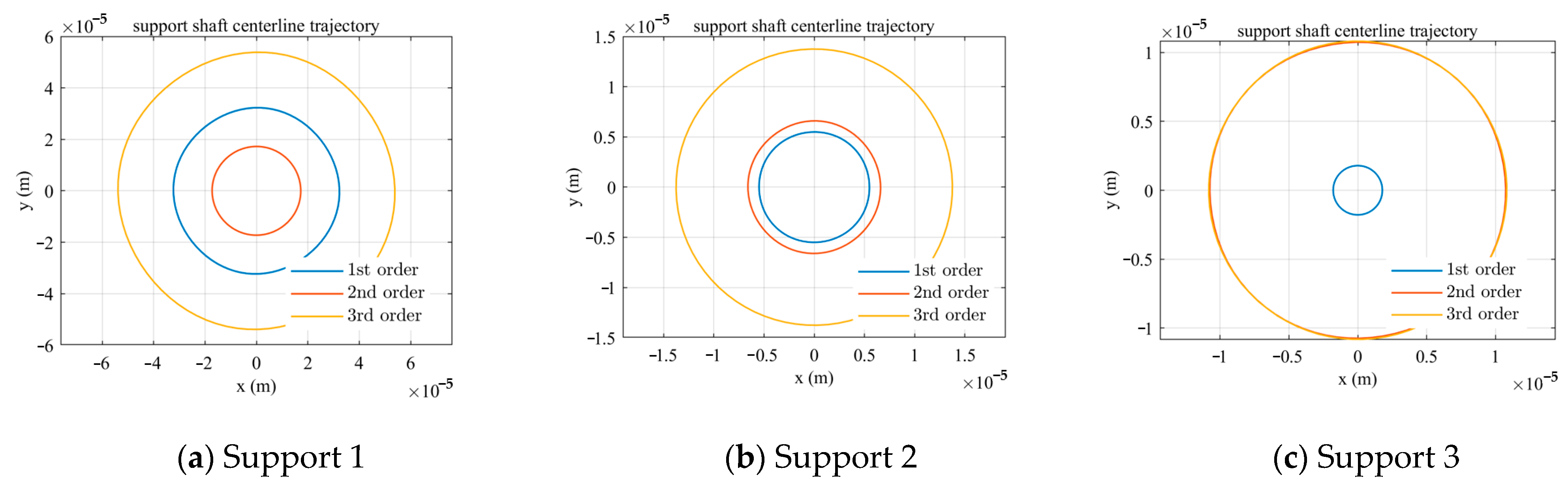
Next, nonlinear oil film forces and nonlinear restoring forces were applied to the three bearings, respectively. The data for the forces applied are as follows: (1) Support 1(C = 5.5 × 10⁻⁵, k_bnl = 1 × 10⁸); (2) Support 2(C = 1.4 × 10⁻⁵, k_bnl = 8 × 10⁸); (3) Support 3(C = 1.1 × 10⁻⁵, k_bnl = 2 × 10⁹).

The axial trajectories of the three bearings are shown in Figure 21. It can be observed that after applying both nonlinear forces (oil film and restoring), bearing 1 exhibits the disappearance of bi-stability near the third critical speed, with its axial trajectory returning to a perfect circle; bearing 2 maintains a perfect circular axial trajectory even after applying both nonlinear forces; and for bearing 3, the amplitudes and axial trajectories near the second and third critical speeds tend to converge, but the third-order trajectory shows slight irregularity.

5.5. Confirmatory Experiment

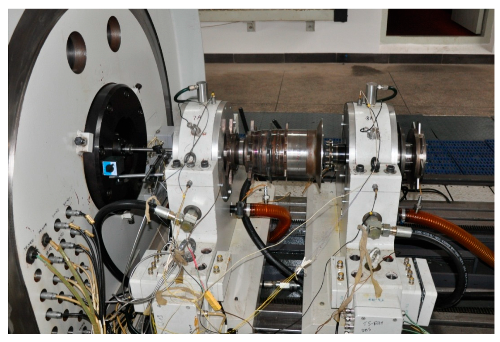
To verify the correctness of the unbalance response law for the SFD-containing rotor model proposed in this paper, and due to the high cost of actual rotors, an experimental test on unbalance response was conducted using a rotor test rig with SFD as shown in Figure 22.

The test equipment was the B768 High-Speed Rotor Dynamic Test Rig, with the rotor adopting a 1-1-0 bearing support scheme. The front support point (compressor end) was equipped with a single-row ball bearing combined with an elastomeric support and squeeze film damping device, while the rear support point (turbine end) used a single-row roller bearing combined with the same damping system. The vacuum chamber pressure was maintained at ≤200 Pa. Two acceleration sensors (A₁ and A₂ at the compressor end, A₃ and A₄ at the turbine end) were installed on each support bracket to measure vertical and horizontal vibration accelerations, respectively: A₁ and A₃ were mounted vertically, while A₂ and A₄ were positioned horizontally. Additionally, one vibration velocity sensor (V₁ at the compressor end, V₂ at the turbine end) was installed in the vertical direction of each support bracket to measure vertical vibration velocities. 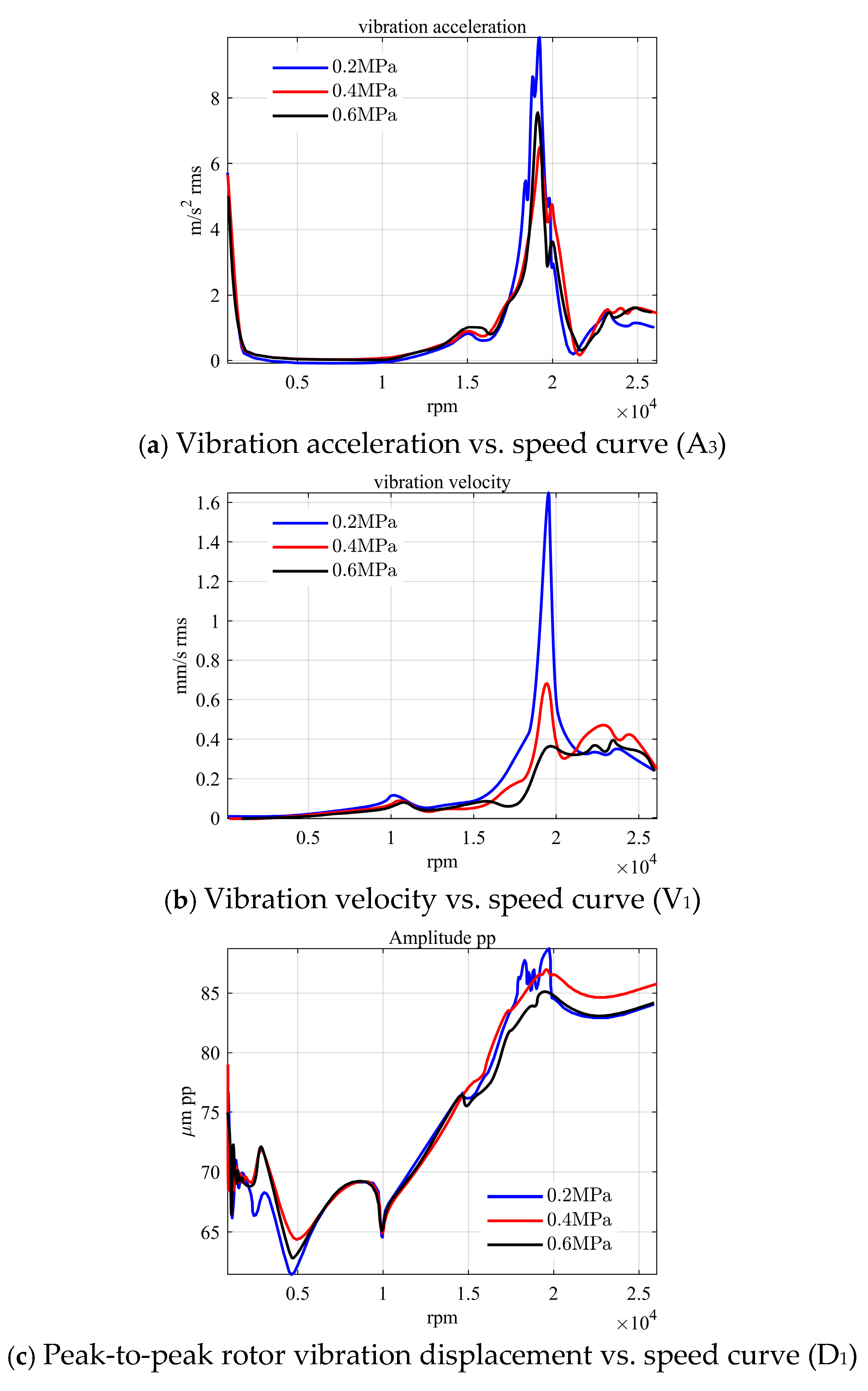Vibration displacement sensors D₁–D₃ were placed on the turbine disk, the vicinity of the rear support bracket’s rotor shaft, and the compressor disk to capture the rotor’s vibration deflection. The SFD oil film force magnitude was adjusted by varying the supply oil pressure of the squeeze film dampers. Tests were conducted at speeds ranging from 0 to 35,000 r/min and supply oil pressures of 0.2 MPa, 0.4 MPa, and 0.6 MPa, measuring the vibration acceleration and vertical vibration velocity at both support brackets (as shown in Figure 23).

Increasing the supply oil pressure is equivalent to enhancing the SFD’s nonlinear oil film force in simulation experiments. The experimental results show that as the oil pressure increases, the damping performance of the supports is enhanced, effectively suppressing the bi-stable phenomenon (Figure 23c, where the nonlinear jump disappears with increasing pressure). This observation aligns with the simulated results where the coupling of two nonlinear forces improved the damping performance of the supports and eliminated the bi-stable instability. The experiments validate the correctness of the unbalance response law in SFD-equipped rotor systems and confirm that the dynamic response mechanism proposed in this study can effectively control the vibration of modern aero-engine rotors. For instance, based on the identified influence law of SFD’s nonlinear oil film force, adjusting parameters such as the oil supply pressure can suppress the rotor’s nonlinear jumping behavior; furthermore, increased oil film force significantly reduces rotor vibration (Figure 23b), demonstrating the practical applicability of the proposed theory.

6. Conclusions

Based on the Euler–Bernoulli beam theory, this paper employs the finite element method to establish a dynamic model of the rotor-support system. The vibration equations for the lumped mass element, the squeeze film damper (SFD) element, and the support element are derived, with the linear components incorporated into the stiffness matrix, mass matrix, and gyroscopic matrix. The nonlinear components are treated as loads and written into the load matrix along with the excitation, thus constructing the overall vibration equation of the model. Subsequently, the Campbell diagram and critical speeds of the rotor are solved using both custom code and ANSYS software, and a comparison between the two validates the correctness of the finite element model coded. Considering the impact of nonlinearity, the Newmark Beta method is selected to solve the time-domain response of the rotor system. Four different scenarios were designed: (1) without nonlinear forces, (2) with SFD nonlinear oil film forces, (3) with support nonlinear restoring forces, and (4) the combined effect of SFD nonlinear oil film forces and support nonlinear restoring forces on the rotor response. The latter three scenarios were compared with the first to investigate the influence of nonlinear forces on the rotor model response.

From this, the following conclusions are drawn:

• Squeeze film dampers can effectively reduce the amplitude of the rotor, and the smaller the oil film clearance C, the more significant the reduction in amplitude. However, it is crucial to select an appropriate range for the oil film clearance to prevent the occurrence of a bi-stable phenomenon, which can compromise the stability of rotor vibration. When the amplitudes of two critical speeds are close, the selection of SFD parameters must be made with caution to avoid an increase in amplitude. The addition of an SFD at the first support resulted in a bi-stable phenomenon, and it was observed that as the oil film clearance C increased, the frequency range affected by the bi-stable phenomenon gradually decreased until it ceased to be an issue. The introduction of an SFD at the third support led to an increase in amplitude. This was due to the proximity of the second-order critical speed amplitude to the third-order amplitude, under the influence of the SFD, the second-order amplitude decreased while the third-order amplitude increased.
• Support nonlinear forces induce a frequency shift in critical speeds, with an observed increase in frequency across all three supports. The impact of support nonlinear forces on amplitude varies among the supports. At the first support, the amplitude on third-order critical speed increases with the augmentation of the support nonlinear force coefficient; when k_bnl = 1 × 10⁸, the amplitude increases by 4%. At the second support, the third-order critical speed amplitude decreases with the increase in the support nonlinear force coefficient; when k_bnl = 8 × 10⁸, the amplitude near the third-order critical speed decreases by 11%. At the third support, both the second and third-order critical speed amplitudes increase with the support nonlinear force coefficient; when k_bnl = 2 × 10⁹, the amplitude near the second-order critical speed increases by 17%, with a corresponding increase in critical speed of 3.5 Hz, and the amplitude near the third-order critical speed increases by 11%.
• The combined effect of the two types of nonlinear forces on the rotor is found to be a simple superposition of the results obtained when each force is applied individually. When both nonlinear forces are added to the first support, the frequency changes are consistent with those observed when only the support nonlinear force is applied, with an increase in amplitude and the disappearance of the bi-stable phenomenon. At the second support, the addition of both nonlinear forces results in a significant reduction in amplitude; compared to the scenario without nonlinear forces, the amplitude at the third-order critical speed decreases by 19%, and the peak frequency increases by 2 Hz. At the third support, the behavior is slightly different from the previous cases, the support nonlinear force increases the second-order critical speed, and the amplitudes of the second and third orders become closer. Upon the addition of the SFD, the second-order amplitude decreases while the third-order amplitude increases, with both being constrained to the same value by the SFD.
• The selection of the location to apply for the SFD significantly influences its effectiveness. In the study of the three supports examined in this paper, the supports located at the ends of the rotor exhibited bi-stable phenomena and an increase in amplitude upon the addition of an SFD. In contrast, the support positioned in the middle of the rotor demonstrated a pronounced vibration reduction effect; the third-order amplitude decreased by 19% compared to the condition without the application of nonlinear forces.