Research on Quasi-Zero Stiffness Vibration Isolation System of Buckled Flexural Leaf Spring Structure for Double Crystal Monochromator

Abstract

The double crystal monochromator (DCM) is a spectrometer in synchrotron radiation beamlines, and its stability directly impacts the quality of the emitted light. In order to meet the requirements of the fourth generation of synchrotron light sources, researchers have designed a DCM using an active control method to ensure stability by actively compensating for crystal displacement through voice coil motors. The active control method imposes high demands on the vibration isolation performance of the DCM frame. In response to external excitation characteristics, this paper proposes a quasi-zero stiffness (QZS) isolation system based on a compressed buckling beam structure. Random vibration simulations using finite element analysis revealed that, under different operating conditions, the 3σ displacement of the core part of the DCM is maintained at the nanometer level. Moreover, this paper presents a calculation method based on elastic potential energy to establish force equilibrium equations for negative stiffness and analyzes stress distribution in the beam during vibration using the derived deflection curve. Validation through finite element simulations confirms the method’s accuracy in calculating negative stiffness and stress distribution. Because of the structural similarities, some of the results of this paper can be applied to the study of negative stiffness honeycomb materials.

1. Introduction

Synchrotron radiation refers to electromagnetic waves emitted by free electrons moving at speeds close to the speed of light, under the influence of a magnetic field, and emitted along the tangential direction of their trajectory, as show in Figure 1. Its spectral range covers from infrared to hard X-rays. Synchrotron light exhibits characteristics such as continuous spectrum, short pulse duration, broad-spectrum, high collimation, high polarization, high purity, and high brightness. Therefore, synchrotron light sources are crucial research tools in fields such as biology, materials science, and medicine.

Synchrotron light is a continuous spectrum polychromatic light, and most experiments require wavelength selection or continuous scanning within a specific range. Therefore, in practical applications, monochromators are commonly used for wavelength selection. For beams ranging from below 2 nm to the hard X-ray region, crystal monochromators are widely used as spectrometers. Their operating principle is based on the Bragg diffraction equation, adjusting the Bragg angle to select specific wavelengths [1,2]. Angular stability is one of the key performance indexes of the double-crystal monochromator, and its precision directly affects the energy of the outgoing light, the stability of the luminous flux, and the stability of the spot location [3]. In beamlines, the distance from the DCM to the sample under test is typically from 10 to 20 m. Minute angular rotations of the crystals in the Pitch direction, on the order of arcseconds, can cause micron-level displacements of the light spot on the sample, and affect the accuracy of the Bragg angle [4,5,6]. With the continuous development of synchrotron applications and the construction of fourth-generation synchrotron light sources, existing DCMs in third-generation synchrotron light sources are no longer able to meet the stability requirements of these advanced sources.

To enhance the stability of the monochromator crystals, vibration is a critical factor to address. Sources of vibration include turbulence, vaporization, and pump-induced oscillations within the cooling system of the first crystal. When multiple sources of excitation overlap, the vibrations of the cooling system become highly complex, making it challenging to suppress these vibrations effectively. Additionally, operational activities surrounding the monochromator can introduce vibrations [7,8,9]. To tackle the stability issues of the monochromator, it is essential to develop a vibration isolation system capable of simultaneously attenuating vibrations from both the cooling system of the crystals and external facility operations.

The DCM requires isolation from vibrations ranging from several hertz to several hundred hertz. For this requirement, a quasi-zero stiffness (QZS) isolation system can be chosen. A QZS isolation system is a low-frequency isolation system composed of parallel positive stiffness and negative stiffness components. When the system is at rest, the positive stiffness component provides support to maintain stability. During dynamic operation, the negative stiffness component counteracts the stiffness of the positive stiffness component. The connection stiffness of the system is close to zero, so as to reduce the transmission of force in the vibration process and achieve the purpose of vibration isolation [10,11,12]. QZS vibration isolation technology was born in the late 1990s to early 2000s, and its design ideas are generally categorized as follows, for example, using tilting springs [13,14], scissors [15,16,17], or cam [18,19,20] structures to achieve QZS effect. Another method is to use the restoring force of a compression flexure beam to provide negative stiffness, which is combined with positive stiffness elements to form a QZS system [21,22,23]. Still another more specialized form is the use of magnetic fields to generate negative stiffness, which is highly nonlinear in this type of structure [24,25,26].

At present, the field of QZS vibration isolation has produced many excellent research outcomes. For example, in terms of structural and material innovations, Lei Xiao et al. studied a QZS system based on 3D-printed soft resin materials. Due to the damping properties of the resin material itself, this structure achieved superior vibration isolation performance and robustness to excitation level changes within the low-frequency range [27]. Xin Liu et al. proposed a compact one-dimensional QZS metamaterial composed of conical shell structural units featuring adjustable bandgaps. This structure offers advantages such as small size, light weight, compactness, and high reliability. The isolation starting frequency was achieved at 15.01 Hz, exhibiting good vibration isolation performance [28]. Chunyu Zhou et al. introduced a QZS isolator with dual-arc-shaped flexible beams. This structure can adapt to different vibration isolation requirements, achieving the desired isolation performance by merely modifying the assembly parameters. Additionally, the structure can accommodate load variations within 10% and provides excellent vibration isolation for excitations above 4 Hz [29]. Haodong Zhou et al. proposed a QZS system based on a conical origami structure. The research showed that this structure, compared to existing QZS isolators, has a broader isolation bandwidth, a lower starting frequency, and reduced transmissibility, demonstrating superior isolation performance, particularly at low frequencies [30].

The QZS vibration isolation system studied in this paper uses fixed-end buckling leaf springs as the negative stiffness element, which is structurally different from the aforementioned research results. Therefore, theoretical studies must refer to other relevant outcomes. Several studies are structurally similar to the QZS negative stiffness elements studied in this paper. For instance, Xiaolong Zhang et al. designed a new hyperbolic QZS structure with nonlinear stiffness, integrating a pair of cosine beams (negative stiffness elements) and a pair of arc beams (positive stiffness elements) for low-frequency vibration isolation. The research showed that the required positive, zero, or negative stiffness could be achieved by selecting appropriate geometric parameters [31]. Size Ai et al. proposed using B-spline beams as negative stiffness elements, derived the B-spline beam configuration, and discussed the relationship between the beam’s geometric parameters and mechanical properties. Finite element simulations and experiments proved the B-spline beam’s negative stiffness structure to be repeatable and efficient in terms of energy absorption [32].

The QZS vibration isolation system studied in this paper uses fixed-end buckling leaf springs as the negative stiffness elements, which is structurally different from the aforementioned research results. As shown in Figure 2, most studies with structures similar to this one use the configuration shown in Figure 2a to achieve compression buckling. These studies have also made significant progress in the study of negative stiffness. For example, Changqi Cai et al. theoretically predicted the negative stiffness of compressed buckling beams under large deformation conditions using the elliptical integral method. The experimental results showed that the negative stiffness values calculated using this method had high accuracy [33]. However, in this type of negative stiffness element, the compression amount is entirely dependent on the structural size parameters and is not an adjustable design variable. In this paper, the configurations shown in Figure 2b,c are used, where the compression amount is treated as an independent design variable that can be freely adjusted in applications. Therefore, the structure studied in this paper cannot directly use the elliptical integral method to solve the negative stiffness calculation problem.

There are relatively few studies with negative stiffness elements with the same structure and boundary conditions as those in this paper. For example, Wu Qian et al. used a nickel–titanium memory alloy temperature-controlled QZS isolation system, in which the nickel–titanium alloy was used to fabricate a negative stiffness element of a cosine beam, whose dynamics could be controlled by changing the temperature through electrical heating [34]. Liu Ji et al. designed a cell that could satisfy the optimal QZS performance and the smallest size at the same time through the combination of a positively stiffened cardioid beam with a negatively stiffened cosine beam, and the vibration isolator made up of the cell can isolate vibrations from 3.2 to 60 Hz [35]. Pascal Fossat et al. conducted vibration isolation tests using a 3D-printed QZS system, employing fixed-end compressed buckling plastic beams as the negative stiffness elements, confirming the negative stiffness effect of this structure [36]. Similarly, Benjamin A. Fulcher et al. used 3D-printed structures for experiments and derived a complete formula for calculating negative stiffness. However, the results showed significant discrepancies between the theoretical negative stiffness values and experimental results [37]. If the material is changed from plastic to spring steel, the discrepancy increases with the rise in elastic modulus. The reason for the error is that the relationship between preload force and compression after beam buckling was not derived, resulting in inaccurate preload force values during calculations, with the preload force error being positively correlated with the amount of compression.

This paper primarily addresses the vertical vibration isolation issues of the DCM. Based on a quasi-zero stiffness isolation system, it designs a vibration isolation system suitable for ultra-high stability DCMs. The system integrates positive stiffness helical springs in parallel with negative stiffness compressed buckling LSs. This study involves in-depth research into quasi-zero stiffness theory and enhances the calculation method for the negative stiffness values of compressed buckling Euler beams fixed at both ends. Compared to traditional methods, this approach significantly improves the accuracy of negative stiffness value calculations. In this paper, we conduct thorough analyses of its static and dynamic characteristics through theoretical calculations and finite element simulations, culminating in vibration transmission and random vibration response analyses.

2. Vibration Isolation System of the DCM

The working principle of a DCM involves using Bragg diffraction to extract monochromatic light from the continuous spectrum of synchrotron radiation that is tailored for experimental needs. With the increasing brightness of third- and fourth-generation synchrotron light sources, the power density on the crystal surface of monochromators can reach several tens of watts per square millimeter. Thermal loads can cause local protrusions on the crystal, overall warping, and changes in lattice constants, leading to decreased surface accuracy of the crystal. Therefore, it is essential to incorporate a cooling system to ensure the thermal stability of the crystals.

The DCM cooling system creates vibrational excitation of the crystal; the root mean square angular vibration amplitude of the crystals can reach several hundred nrad. However, fourth-generation synchrotron light sources require the angular stability of crystals to be about 15–30 nrad, i.e., the relative angular displacement between the first and second crystals, as shown in Figure 3, should not exceed 15–30 nrad.

The traditional DCM to solve the problem of crystal angular stability is to obtain a higher angular displacement resolution to ensure the precision of the Bragg angle through the high rigidity mechanical shaft and stepping motor or piezoelectric drive. Therefore, the traditional DCM mainly through the optimization of the mechanical structure to reduce the crystal amplitude to ensure the angular stability; however, through the optimization of the mechanical structure, it is difficult to meet the stability requirements of the fourth generation of light sources [38].

In order to meet the requirements of the fourth-generation light source, scholars proposed a new design method: using a laser interferometer to measure the crystal angular displacement and completing the active control by driving the crystal rotation to keep the crystal angle stable through the voice coil motor, as show in Figure 4. Active control methods enable the DCM to meet the 15–30 nrad angular stability requirement. The frame also needs to have stronger vibration isolation to prevent vibration excitation (external vibration) from the cooling system and peripheral facilities from being transmitted to the active regulating mechanism (core element) to affect its regulating accuracy.

Key parameters affecting vibration isolation performance include the damping ratio and natural frequency. When the external excitation amplitude A and the frequency ratio ω/ω_n (where ω is excitation frequency and ω_n is natural frequency) exceed $\sqrt{2}$, increasing the damping ratio ξ increases the steady-state response amplitude X of the system, but the transmissibility X/A remains less than one. Conversely, when the frequency ratio is less than $\sqrt{2}$, increasing the damping ratio reduces the steady-state response amplitude, while the transmissibility remains greater than one, as show in Figure 5. The natural frequency of the isolation system is primarily influenced by stiffness k and mass m, as shown in Equation (1).

$${\omega }_n=\sqrt{{\displaystyle \frac{k}{m}}}$$

(1)

$${\displaystyle \frac{X}{A}}={\displaystyle \frac{\sqrt{1+{\left(2\xi \frac{\omega }{{\omega }_n}\right)}^2}}{\sqrt{{\left[1-{\left(\frac{\omega }{{\omega }_n}\right)}^2\right]}^2+{\left(2\xi \frac{\omega }{{\omega }_n}\right)}^2}}}$$

(2)

Reducing the natural frequency of the system effectively isolates the external vibration excitation, which can be achieved by increasing the mass of the DCM or by reducing the stiffness of the frame connection. For the DCM, due to the limitation of the mass of the base frame, reducing the stiffness is a more practical way to achieve the same natural frequency; therefore, a quasi-zero stiffness isolation system is chosen for the frame vibration isolation design.

The operating principle of a QZS system involves using a positive stiffness component to support the weight of the isolated component, while a negative stiffness component counteracts the positive stiffness during vibrations. In static conditions, the system has sufficient static stiffness to maintain stability, while, during dynamic processes, the stiffness approaches zero, maintaining a low natural frequency. The design focus of QZS systems lies in the negative stiffness element, commonly implemented with spiral compression springs or compression-bent beams or leaf springs (LSs).

Due to the spatial constraints of the DCM and the requirement for a thin isolation system in a high vacuum environment, only an LS structure can meet these demands. Therefore, using buckled LSs with fixed ends as the negative stiffness element is ideal for such applications as it involves no moving parts and requires no lubrication, making it suitable for vacuum environments. Although this form of quasi-zero stiffness isolation is only effective for vibrational excitation in one direction, the core element of the DCM is mainly sensitive to longitudinal displacements, so quasi-zero stiffness isolation can be applied to this scenario.

In the field of QZS, the traditional method of numerical calculation of the negative stiffness of LSs in the form of fixed ends suffers from a large error, which grows linearly with the change in the elastic modulus of the material. Therefore, academics usually carry out theoretical calculations when using low modulus of elasticity 3D printed plastics to make LSs, for example, the traditional calculation method is widely used in the study of energy-absorbing metamaterials with honeycomb structure. However, for metallic LSs, due to the large calculation errors, designers typically rely on finite element simulations combined with vibration experiments for accurate design. In practical applications, metallic materials are more suitable for LS production. Hence, this paper proposes a new method for calculating negative stiffness values, significantly improving the accuracy of these calculations.

3. Structural Design and Analysis of QZS Vibration Isolation Systems

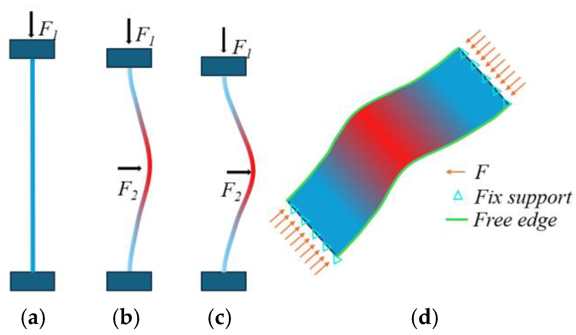
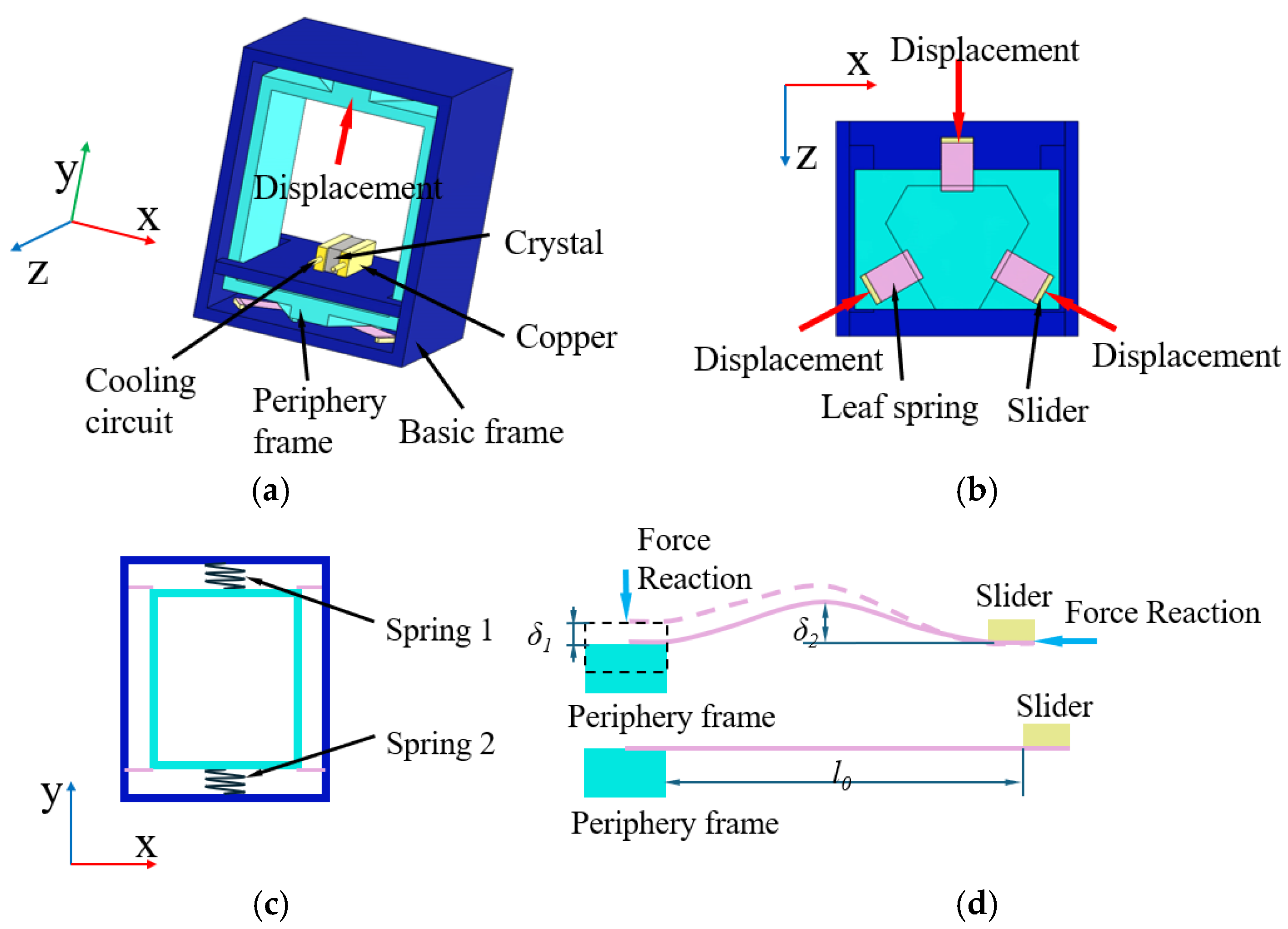
3.1. Negative Stiffness Element Design

The negative stiffness element uses a fixed-end compressed buckling rectangular LS with a stiffness coefficient of k₁. The positive stiffness element uses a helical spring with a stiffness coefficient of k₂. As shown in Figure 6, these two components form a QZS system. After the complete assembly of the DCM, the weight of the periphery frame of the DCM compresses the helical spring, bringing the entire vibration isolation system to a balanced position where the total stiffness of the isolation system is approximately zero. Since the DCM contains precision components, such as voice coil motors and laser interferometer probes, the material used for making the LSs needs to have low magnetic permeability. ANSI301 is suitable as a material for LSs because, compared to other grades of stainless steel, ANSI301 has better strength and lower magnetic permeability, making it ideal for manufacturing elastic components in precision mechanical applications. In addition, DCMs have a strict volume limitation for working scenarios. Buckling leaf springs have a natural advantage in this regard and are better suited for this application than other types of negative stiffness structures.

The rectangular LS plays a crucial role in the QZS system, serving as a key component in the design of the QZS system. Based on the specifications of the vibration isolation system, the length, width, and thickness of the LS are used as design parameters. Considering the practical aspects of manufacturing the LS, the thickness h of the LS is taken as a constant, while the length l₀ or the width b of the LS are treated as variables for design and optimization.

The QZS system, as shown in Figure 7, features an LS that bends into an arch shape under the action of compressive load F. When subjected to external vibrations, the movable end of the LS undergoes a slight displacement δ₁ in the vertical direction. The elastic potential energy of QZS during the dynamic process satisfies the following equation:

$$N\cdot {\displaystyle \frac{\partial U_a}{\partial {\delta }_1}}+{\displaystyle \frac{U_b}{\partial {\delta }_1}}=N\cdot ({\displaystyle \frac{U_c}{\partial u_x}}+{\displaystyle \frac{U_d}{u_x}})\cdot \sin ({\tan }^{-1}({\displaystyle \frac{{\delta }_1}{l_0-u_x}}))$$

(3)

In the equation, U_a represents the elastic potential energy generated by the deformation of the compliant LS due to the amplitude δ₁. U_b represents the elastic potential energy generated by the axial tension and compression of the positive stiffness spring. U_c represents the elastic potential energy generated by the compression of the compliant LS from its planar state (purple curve in Figure 7) to its buckled state (blue curve in Figure 7). U_d represents the elastic potential energy generated by the slight compression of the LS during its buckling process. N is the number of LSs in the QZS system. The terms in Equation (3) require detailed design parameters of the LS for calculation. Therefore, the following research will first establish a simplified force equilibrium equation for preliminary calculations, and the detailed derivation process of Equation (3) (the precise force equilibrium equation) will be presented in later sections.

As shown in Figure 7, the fixed end of the LS is compressed towards the movable end by an amount u_x. After the LS completes the buckling process, it stores elastic potential energies U_c and U_d in the horizontal direction. By differentiating these with respect to the compression u_x, the compressive load F in the horizontal direction is obtained. When subjected to vibration excitation, the movable end of the LS displaces vertically by δ₁. At this point, the positive stiffness spring stores elastic potential energy U_b due to the change in length in the vertical direction, and the LS stores elastic potential energy U_a due to the displacement of the movable end in the vertical direction. Differentiating these with respect to δ₁ yields the elastic forces in the vertical direction, which are opposite in direction to the displacement δ₁.

Furthermore, after the displacement of the movable end of the LS, the direction of the compressive load F of the LS inclines by an angle θ, which is the angle between the line connecting the movable end and the fixed end of the LS and the horizontal line. This causes a component of the compressive load F to act in the vertical direction, in the same direction as δ₁.

Considering these conditions, under external vibration excitation, the system’s response amplitude is δ₁. The forces exerted by the positive stiffness spring and the LS in the vertical direction (left side of Equation (3)) balance with the vertical component of the F from the buckled LS (right side of Equation (3)). Therefore, the force balance equation during the vibration process is obtained as shown in Equation (3). In Equation (3), the U_c term is not calculated using the deflection curve during the vibration process (orange curve in Figure 7) because the deformation of the LS during the vibration process is mainly in the vertical direction, and its compression potential energy remains almost unchanged. Hence, the error introduced by using the equilibrium position’s deflection curve (blue curve in Figure 7) for the calculation is minimal.

In the actual design process, all the dimensional parameters of the LS are required to establish the force balance equation. Therefore, at the initial design stage, the force balance equation needs to be simplified to avoid missing dimensional parameters. After completing the preliminary calculations using the simplified formula, the precise equation can be used for adjustments based on the available conditions. The F of the LS in the horizontal direction is simplified to an unknown quantity P. The elastic potential energy U_a, due to the deformation of the LS in the vertical direction, is relatively small, and, since it cannot be calculated without the dimensional parameters of the LS, it can be temporarily ignored. Thus, Equation (3) simplifies to the following:

$$k_2\cdot {\delta }_1=N\cdot P\cdot \sin ({\tan }^{-1}({\displaystyle \frac{{\delta }_1}{l_0-u_x}}))$$

(4)

The axial compression u_x is typically two orders of magnitude smaller than the initial length l₀. Additionally, the derivatives of the sine and arctangent functions near the origin are approximately one. Therefore, the equation can be approximated as follows:

$$k_2\cdot {\delta }_1=N\cdot P\cdot {\displaystyle \frac{{\delta }_1}{l_0}}$$

(5)

In the operation of the QZS system, the negative stiffness element must always remain in a state of compressed energy storage, meaning it needs to have sufficient compression to prevent the free end displacement from fully extending and losing the negative stiffness effect during vibrations. The prerequisite for the LS to achieve a larger compression amount is that the F must be greater than the critical load P_er for its first mode shape buckling, as shown in Figure 8. There is a nonlinear relationship between the axial compression amount and the compression load, primarily characterized by a stiffness softening effect occurring in the LS’s axial compression once the compression load exceeds P_er. The calculation method for this will be detailed later.

As shown in Figure 8d, the rectangular LS used in the quasi-zero stiffness system has two free edges, which are neither loaded nor constrained. Therefore, its deflection calculation can be equivalent to the deflection calculation of a beam. The critical buckling load for the LS with both ends fixed is given by the following:

$$P_{er}={\displaystyle \frac{4{\pi }^{2}E\frac{b{h}^3}{12}}{{l_0}^2}}$$

(6)

Here, P_er represents the aforementioned compressive load F. Given the critical load P_er, the elastic modulus E of the material, and two of the dimensions among width b, length l₀, and thickness h, the unknown dimensional parameters can be solved using this formula. It should be noted that, to ensure it is greater than P_er, when thickness or width is unknown, the design dimensions should be slightly smaller than the solved result. Conversely, when the length is unknown, the design dimensions should be slightly larger than the solved result. It should be noted that leaf spring thicknesses usually depend on the metal material manufacturer and need to be selected at the design stage based on their factory thickness. Parameter optimization of leaf springs can be performed by using Equation (5) as a baseline and substituting the known parameters as well as the desired value of negative stiffness. Since Equation (5) contains only four design parameters, even if there are several unknown parameters, the range of values can be determined after several attempts of calculation, and, finally, the parameters can be corrected and calibrated by Equation (30), which is a high-precision formula derived in the subsequent chapters.

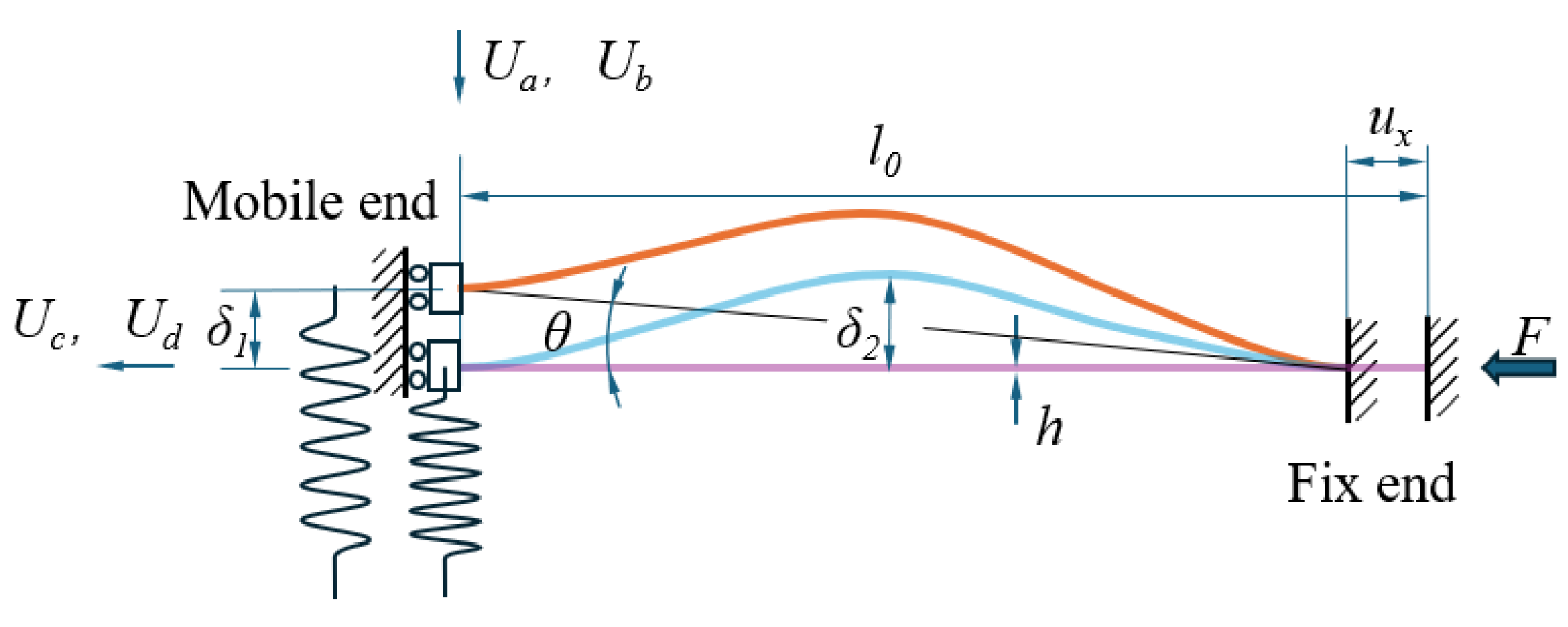
3.2. The Analysis of the Compression of the Leaf Spring

Given the elastic modulus E, width b, length l₀, and thickness h of the LS, we can proceed to calculate the compression amount through the calculation of axial compression potential energy.

The bending strain energy U_c of the beam can be computed using the deflection:

$$U_c={\displaystyle \frac{EI}{2}}{\displaystyle \int {(\frac{d^{2}w}{d{x}^2})}^2}dx$$

(7)

I is the moment of inertia of the beam. For a beam fixed at both ends, its post-buckling deflection curve (blue curve in Figure 7) is as follows [39]:

$$w_1={\displaystyle \frac{{\delta }_2}{2}}(1-\cos {\displaystyle \frac{2\pi x}{l_0-u_x}})$$

(8)

Substitute Equation (8) into Equation (7) and integrate as follows:

$$U_c={\displaystyle \frac{EI{{\delta }_2}^2{\pi }^4}{{(l_0-u_x)}^3}}$$

(9)

The derivative of the potential energy U_c with respect to the compression u_x yields an approximate value of F (the exact value is the sum of the U_c and U_d terms in Equation (3), but the U_d term is several orders of magnitude smaller than the U_c term; here, F can be used as an exact value), but Equation (9) still contains the unknown δ₂. After the beam undergoes flexural deformation, its length L is calculated using the curve length formula:

$$\begin{array}{l}L={\displaystyle {\int }_0^{l_0-u_x}\sqrt{1+{\left(\frac{d{w}_1}{dx}\right)}^2}dx}\\ ={\displaystyle {\int }_0^{l_0-u_x}\sqrt{1+{\left(\frac{\pi {\delta }_2}{l_0-u_x}\sin \left(\frac{2\pi x}{l_0-u_x}\right)\right)}^2}dx}\end{array}$$

(10)

The integral can be approximated as follows [37]:

$$\begin{array}{l}L={\displaystyle {\int }_0^{l_0-u_x}1+\frac{1}{2}{\left(\frac{\pi {\delta }_2}{l_0-u_x}\sin \left(\frac{2\pi x}{l_0-u_x}\right)\right)}^{2}dx}\\ ={\displaystyle \frac{{{\delta }_2}^2{\pi }^2}{4(l_0-u_x)}}+l_0-u_x\approx l_0\end{array}$$

(11)

The beam length L after compression buckling can be approximated to the initial length l₀, as the shortening due to pre-tension is several orders of magnitude lower than l₀. According to Equation (11), the relationship between δ₂ and compression u_x is derived as follows:

$${\delta }_2=\sqrt{{\displaystyle \frac{4u_x(l_0-u_x)}{{\pi }^2}}}$$

(12)

Substituting Equation (12) into Equation (9) and differentiating gives the following:

$$U_c={\displaystyle \frac{4EI{\pi }^2}{{(l_0-u_x)}^2}}{u}_x$$

(13)

$${\displaystyle \frac{\partial U_c}{\partial u_x}}=4EI{\pi }^2\left[{(l_0-u_x)}^{-2}+2{(l_0-u_x)}^{-3}\right]\approx F$$

(14)

Figure 9 shows the relationship between the compression displacement u_x and the F of compliant LSs calculated using Equation (14), compared with finite element simulation results. It is evident that the compression stiffness after buckling may decrease by several orders of magnitude compared to before buckling. This suggests that using buckled LSs as negative stiffness elements has good tolerance to errors in compression displacement, as F is not highly sensitive to compression displacement errors.

3.3. Potential Energy and Negative Stiffness Derivation

In the previous theoretical derivation, all parameters necessary for calculating potential energy have been obtained. In the calculation of compression, the elastic potential energy U_c of the compliant LS was derived from Equation (13). Next, we proceed to calculate the elastic potential energies U_a, U_b, and U_d.

For U_a, we can similarly use the approach in Equation (7): calculating the elastic potential energy of the one end fixed and one end with small displacement (the orange deflection curve in Figure 7) and subtracting the elastic potential energy due to compression alone (the blue deflection curve in Figure 7). For the calculation of the deflection curve with one end fixed and one end with small displacement after compression buckling (the orange deflection curve in Figure 7), the superposition method can be used by superimposing the buckled deflection curve with both ends fixed and one end eccentric on the buckled deflection curve with both ends fixed.

As shown in Figure 10, the moment distribution of a beam fixed at both ends and eccentric at one end is as follows:

$$M=F({\displaystyle \frac{{\delta }_1}{2}}-w_2)$$

(15)

where w₂ is the deflection of the beam. The differential equation for the deflection curve can be obtained from the moment:

$$EI{w^{″}}_2=-M=F({\displaystyle \frac{{\delta }_1}{2}}-w_2)$$

(16)

Using the notation k² = F/EI, Equation (16) becomes the following:

$${w^{″}}_2+k^2{w}_2=k^2{\displaystyle \frac{{\delta }_1}{2}}$$

(17)

The homogeneous solution w_H and particular solution w_H of this equation are as follows:

$$\left\{\begin{array}{l}{w}_H=C_1\sin kx+C_2\cos kx\\ w_P={\displaystyle \frac{{\delta }_1}{2}}\end{array}\right.$$

(18)

Using the boundary conditions, we can obtain the following:

$$\left\{\begin{array}{l}{w}_2(0)=0\\ {\mathrm{w}}_2{(\mathrm{l}}_0{-\mathrm{u}}_x)={\delta }_1\\ {w^{\prime }}_2(0)={ \mathrm{w} \prime }_2{(\mathrm{l}}_0{-\mathrm{u}}_x)=0\end{array}\right.$$

(19)

Substituting into Equation (18) gives the following:

$$\left\{\begin{array}{l}{C}_1=0\\ C_2=-{\displaystyle \frac{{\delta }_1}{2}}\\ k={\displaystyle \frac{\pi }{l_0-u_x}}\end{array}\right.$$

(20)

The deflection equation is as follows:

$$w_2={\displaystyle \frac{{\delta }_1}{2}}(1-\cos {\displaystyle \frac{\pi x}{l_0-u_x}})$$

(21)

As shown in Figure 11, using the superposition method to simply add w₁ and w₂, the deflection curve differs from the finite element simulation results primarily in that the maximum deflection in the finite element simulation is slightly greater than the approximate value. Moreover, the error is larger on the side near the fixed end when δ₁ > 0, whereas the error is larger on the side near the movable end when δ₁ < 0. Since the deflection curve calculated using the superposition method already includes the deflection curve due to buckling alone (the blue deflection curve in Figure 7), the calculation of potential energy U_a can be simplified to the energy stored by the LS bending into the shape w₂ under the moment, thereby omitting the calculation of elastic potential energy due to buckling.

$$\begin{array}{l}{U}_a={\displaystyle \frac{EI}{2}}{\displaystyle \int {(\frac{d^2{w}_2}{d{x}^2})}^2}dx\\ ={\displaystyle \frac{EI{\delta }_1^2{\pi }^4}{16{(l_0-u_x)}^3}}\end{array}$$

(22)

It should be noted that the curve w₂ undergoes compressive buckling in the horizontal direction; however, here, its curve w₂ is calculated only to be superimposed on w₁ in the vertical direction, so the subsequent derivation process only needs to calculate the elastic force of the curve w₂ in the vertical direction. In addition, compression buckling is a large deformation behavior. This leads to some errors in the U_a terms calculated here using the superposition method. The advantage of the superposition method is that the derivation and calculation process is more concise and clear, although the accuracy is slightly lower compared to the elliptic integration method used by Changqi Cai [33]; however, here, the boundary conditions are not sufficient to establish the differential equations needed for the elliptic integration, and, therefore, there is no better method to solve this problem for the time being, so the U_a term will be corrected in later chapters.

The elastic potential energy stored in the positive stiffness spring due to tension and compression is as follows:

$$U_b={\displaystyle \frac{1}{2}}k{\delta }_1^2$$

(23)

Finally, calculate the elastic potential energy U_d stored due to the length compression of the compliant LS. In Equation (11), the length of the LS after compression is computed, subtracting this from l₀ gives the compression length. The elastic potential energy is then given by the following [37]:

$$U_d={\displaystyle \frac{AE}{2l_0}}{\left[u_x-{\displaystyle \frac{{{\delta }_2}^2{\pi }^2}{4(l_0-u_x)}}\right]}^2$$

(24)

Differentiating U_a, U_b, U_c, and U_d, we obtain the following:

$${\displaystyle \frac{\partial U_a}{\partial {\delta }_1}}={\displaystyle \frac{EI{\delta }_1{\pi }^4}{8{(l_0-u_x)}^3}}$$

(25)

$${\displaystyle \frac{\partial U_b}{\partial {\delta }_1}}=k{\delta }_1$$

(26)

$${\displaystyle \frac{\partial U_c}{\partial u_x}}=4EI{\pi }^2\left[{\left(l_0-u_x\right)}^{-2}+2{\left(l_0-u_x\right)}^{-3}\right]$$

(27)

$${\displaystyle \frac{\partial U_d}{\partial u_x}}={\displaystyle \frac{AE}{2l_0}}\left[2u_x-{\displaystyle \frac{{\delta }_2^2{\pi }^2}{2\left(l_0-u_x\right)}}-{\displaystyle \frac{{\delta }_2^2{\pi }^2{u}_x}{2{\left(l_0-u_x\right)}^2}}+{\displaystyle \frac{{\delta }_2^4{\pi }^4}{8{\left(l_0-u_x\right)}^3}}\right]$$

(28)

The numerical value of δ₂ in Equation (28) can be calculated using Equation (12). The equilibrium condition in Equation (3) states that the zero-stiffness system is composed of a positive stiffness spring and a negative stiffness component. Therefore, by substituting material parameters and dimensional parameters into Equation (3), the stiffness coefficient k required for the spring in the zero-stiffness system can be determined, where the stiffness coefficient k₁ = −k for the negative stiffness component.

$$k_1=N{\displaystyle \frac{\frac{\partial U_a}{\partial {\delta }_1}-(\frac{\partial U_c}{\partial u_x}+\frac{\partial U_d}{\partial u_x})\cdot \sin ({\tan }^{-1}(\frac{{\delta }_1}{l_0-u_x}))}{{\delta }_1}}$$

(29)

From Equation (29), it can be seen that the negative stiffness k₁ is influenced by the displacement δ₁ during vibration, as shown in Figure 12. The numerical value of the negative stiffness is relatively insensitive to the displacement, hence, in calculations, a small displacement value can be arbitrarily chosen to determine the numerical value of the negative stiffness.

4. Finite Element Analysis

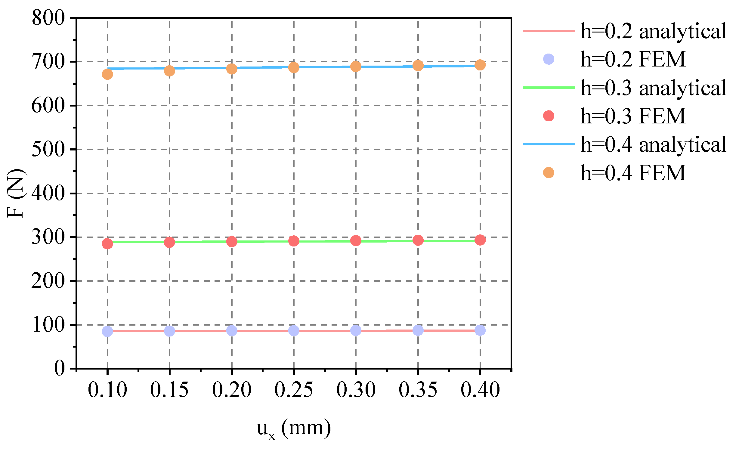
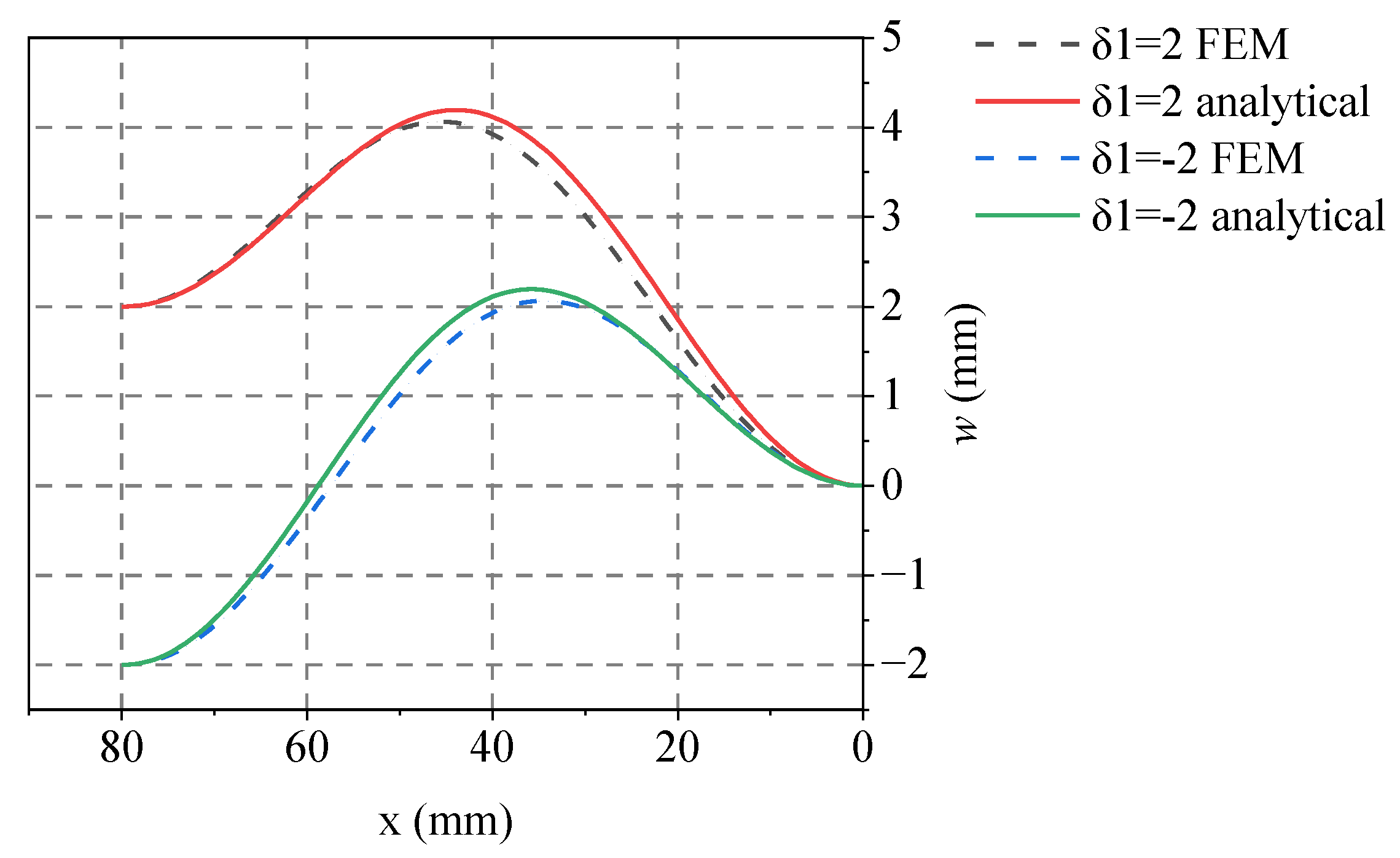
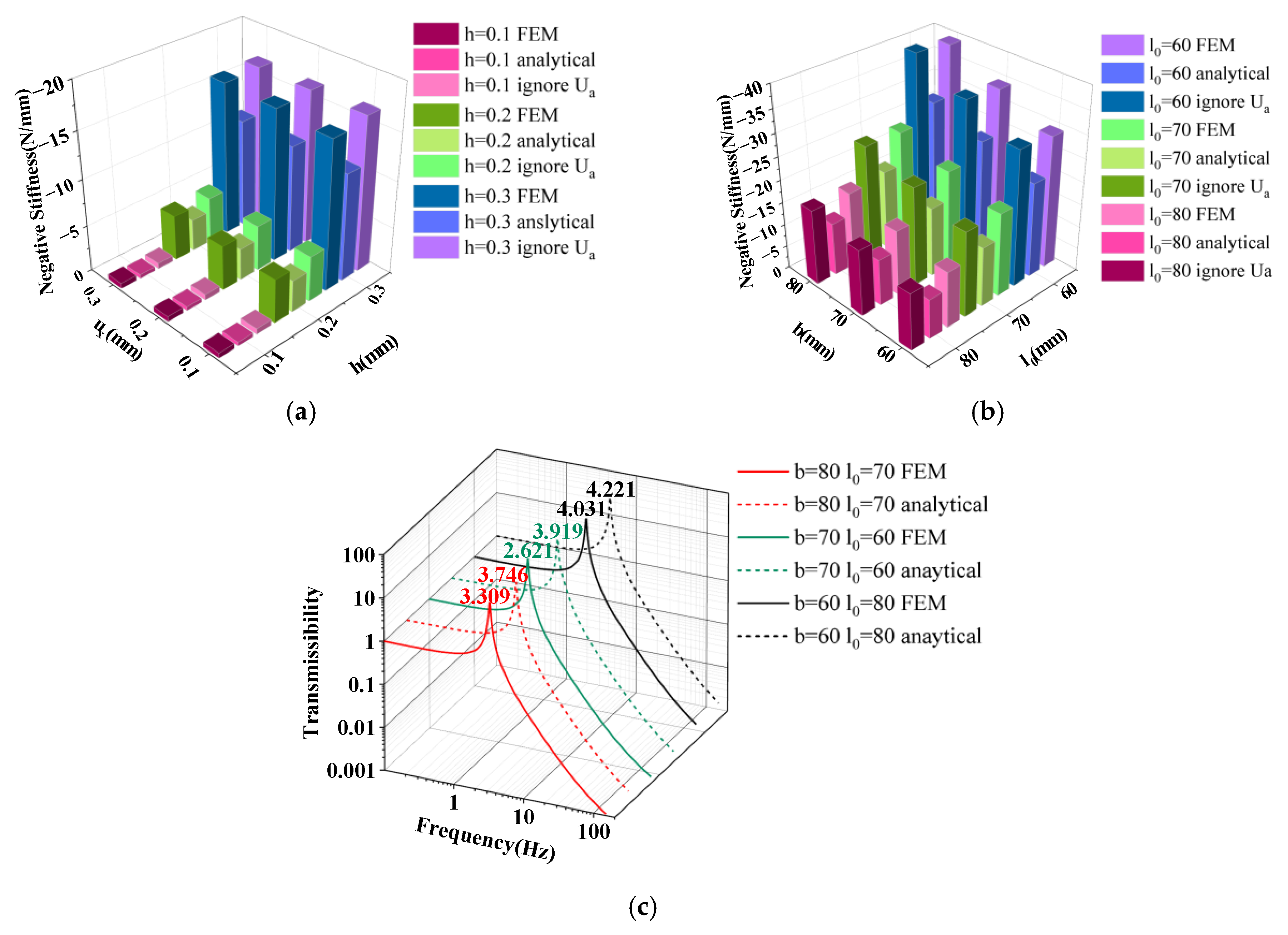
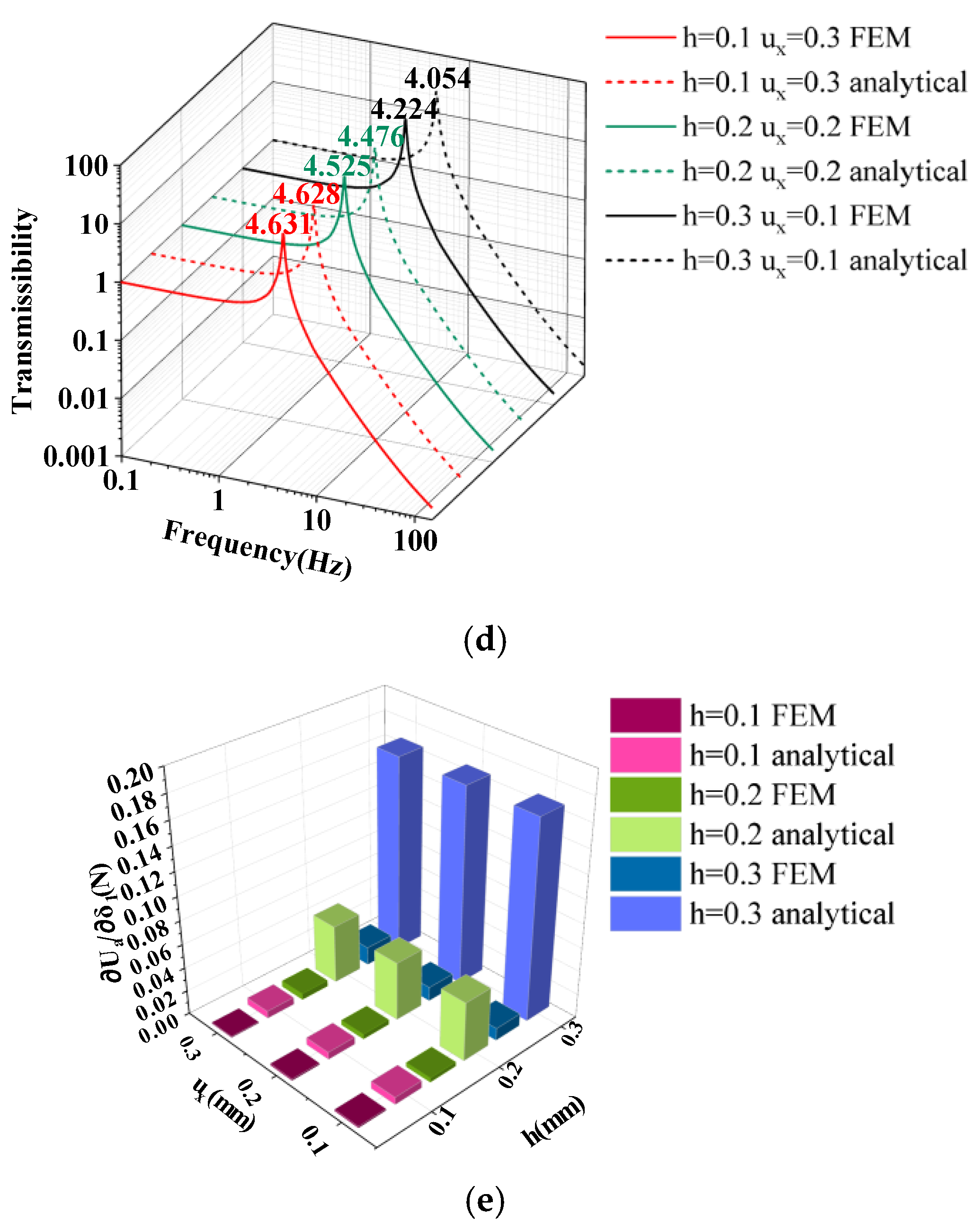
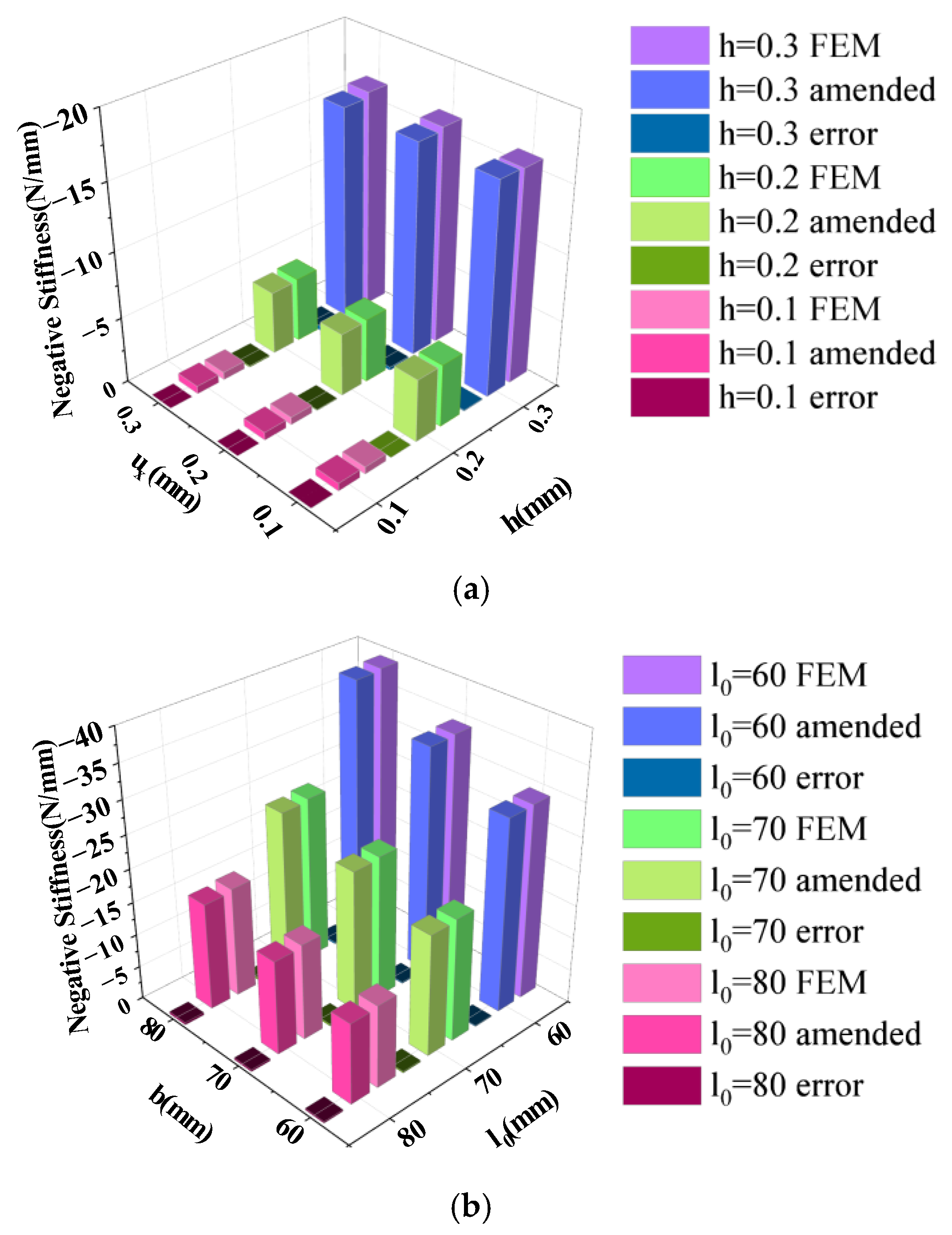
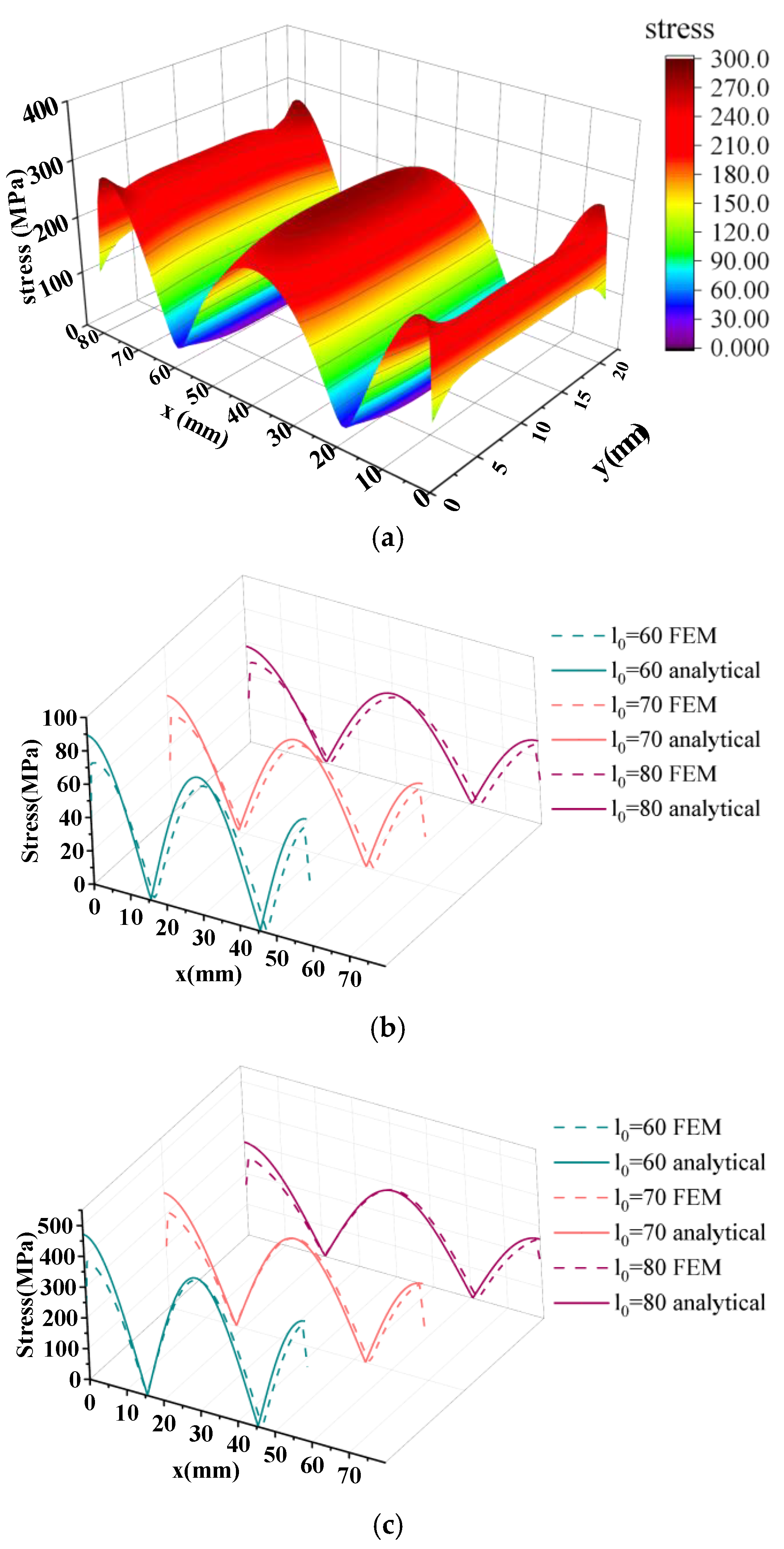
4.1. Accuracy of Formulas

The verification of Equation (29) was mainly conducted through finite element simulations using software such as HyperWorks 2019, ANSA v24.0.0, ANSYS APDL, and ANSYS Workbench 2023R1. Numerical simulations in statics and harmonic response were performed to verify the calculated negative stiffness values and transmissibility derived from Equation (29). In the previous section on the derivation of the U_a term we showed that the superposition method produces errors for large deflection behavior and that there is no better solution for the time being because of the boundary condition problem, so finite element simulations will be used as a reference point here as a way to correct the U_a term.

The finite element model is shown in Figure 13. The structure mainly consists of a crystal assembly, a basic frame, a peripheral frame, and LSs. The number of LSs is 6. One end of the LS is connected to the peripheral frame and the other end is connected to the basic frame through a slider. The key parameters of the LS are shown in

Table 1. Dimensions and material properties of LSs.

Parameter	Value
Length (mm)	60	70	80
Width (mm)	60	70	80
Thickness (mm)	0.1	0.2	0.3
Compression (mm)	0.1	0.2	0.3
Elastic Modulus (GPa)	193
Poisson’s Ratio	0.28

. The compression of the compliant LSs is achieved by applying a displacement boundary to the slider, while the force transfer between the LSs and the slider contact pair is measured using a force response probe. The force transfer between the plate spring and the slider is equal to the F illustrated in Figure 7, and these data are measured in order to solve for the value of the U_a term in the finite element simulation in the next calculation. A total of two springs with a stiffness of 25 N/mm were used for the connection of the basic frame to the peripheral frame, with a total positive stiffness of 50 N/mm and a mass of 58.5 kg for the peripheral frame.

The calculation method for negative stiffness values is as follows: In the Static Structural module, firstly, compression buckling of the LS is achieved through slider displacement. Secondly, the peripheral frame is driven to move along the y-axis using displacement boundary conditions, and the force reaction probe measures the force required for this displacement boundary condition. Finally, the actual stiffness value is obtained by dividing the force reaction of the peripheral frame by the displacement distance. The negative stiffness value is then derived by subtracting the positive stiffness value from the actual stiffness value. The role of the force reaction probe here is to measure the driving force required for the peripheral frame to move a specified distance along the y-axis. Using force to drive peripheral frame displacement can also calculate stiffness values, but it is less effective in terms of solution speed and convergence compared to using displacement boundary conditions.

The simulation of transmissibility involves three modules: Static Structural, Modal, and Harmonic Response. The analysis process is as follows: First, compression buckling of the LS is completed in the Static Structural module. Second, the first six modal frequencies of the entire structure after buckled are computed. Third, 1 g acceleration excitation is applied to the base of the basic frame in the harmonic response. The response amplitudes of the base frame and peripheral frame are solved using modal superposition. Finally, the transmissibility is obtained by dividing the response amplitude of the peripheral frame by that of the base frame.

Figure 14 presents the comparison between partial finite element simulation results and theoretical values. Figure 14a,c shows the results of negative stiffness and transmissibility calculated for LSs of h = 0.3 and u_x = 0.3, with different lengths l₀ and widths b. Figure 14b,d shows the results of negative stiffness and transmissibility calculated for LSs of l₀ = 80 and b = 80, with different thicknesses h and compression amounts u_x. In theoretical calculations and finite element simulations of negative stiffness values, δ₁ is taken as 0.2 mm. Considering the finite element analysis and subsequent experiments, using a larger value of δ₁ gives more intuitive results, and the millimeter-scale is also convenient to measure during the experiments, so the millimeter-scale δ₁ is used in the subsequent hydrostatic part of this study. As mentioned in the previous study on Equation (29), the numerical magnitude of δ₁ has basically no effect on the accuracy of the calculation of the negative stiffness, and, thus, the negative stiffness calculated using the millimeter-scale δ₁ can still be applied to the DCM.

Figure 14e displays the numerical calculation of force U_a for LSs with l₀ = 80 and b = 80. There is a significant discrepancy between theoretical values and finite element results, which increases with increasing LS thickness. The numerical calculation of U_a in the finite element simulation uses Equation (29), where the sum of terms U_c and U_d equals the force transmission value due to contact between the LS and the slider in the simulation steps mentioned above. Given the values of k₁, δ₁, l₀, and u_x, the U_a term is deduced.

From the comparison of finite element simulation results, it is observed that the error in theoretical calculations of negative stiffness values increases with thickness. As mentioned earlier in the derivation of the U_a term, there will be some error in using the superposition method for large deflection behavior; Figure 14a,b shows that the negative stiffness values calculated after neglecting U_a are closer to the finite element simulation results; the reason for this may be that there is a stiffness softening effect along the normal deformation of the beam after compression buckling as well, and the computation by the superposition method does not take into account the stiffness softening very well. Changqi Cai [33], for other structures with negative stiffness elements, used the elliptic integration method to solve this problem; however, because of the limitation of the boundary conditions, the study in this paper is unable to establish the differential equations required for elliptic integration.

Although the inclusion of U_a introduces errors, neglecting U_a in theoretical calculations results in a slightly weaker negative stiffness effect than in reality. Designing based on formulas that neglect U_a may result in an overall negative stiffness even when the LS is connected in parallel with positive stiffness springs. To avoid design errors, the influence of U_a must be considered during calculations.

Based on comparisons of 81 sets of finite element simulations and theoretical calculations, it was found that the theoretical values of U_a are approximately one order of magnitude larger than the simulated values. Therefore, a correction factor of 0.1 is applied to U_a. Because, at this stage, the finite element simulation technology has achieved a better accuracy after years of development, in order to make the subsequent experiments have a better reference basis the correction factor here is based on the finite element simulation results and the subsequent chapters will be verified through experiments to see if the corrected formula is accurate.

As shown in Figure 15, Figure 15a presents the results of negative stiffness calculated for an LS of l₀ = 80 and b = 80 with different thicknesses h and compression amounts u_x, while Figure 15b shows the results of negative stiffness calculated for an LS of h = 0.3 and u_x = 0.3 with different lengths l₀ and widths b. After the correction of U_a, the calculated values of negative stiffness closely match the finite element results, and the accuracy of the results is minimally affected by dimensional parameters such as length and width.

Equation (29) is modified as follows:

$$k_1=N{\displaystyle \frac{0.1\cdot \frac{\partial U_a}{\partial {\delta }_1}-(\frac{\partial U_c}{\partial u_x}+\frac{\partial U_d}{\partial u_x})\sin ({\tan }^{-1}(\frac{{\delta }_1}{l_0-u_x}))}{{\delta }_1}}$$

(30)

After summarizing the theoretical calculation results, it was found that, compared to the values of U_a and U_c, the value of U_d is several orders of magnitude smaller and involves higher computational complexity. It is also highly sensitive to the accuracy of u_x and δ₂. Therefore, U_d can be ignored in the calculations. This approach introduces an error in the negative stiffness values typically on the order of one in ten thousand, which is negligible in terms of computational accuracy.

4.2. Stress Field Analysis

According to Equation (30), F is a cubic function of LS thickness. Therefore, the negative stiffness value of quasi-zero stiffness systems is primarily influenced by the thickness of the LS. Beams exhibit significant deflection accompanied by high stress, and the maximum stress value is linearly related to the beam’s thickness. Thus, in the design of quasi-zero stiffness systems, it is crucial to prioritize LS thickness to meet strength requirements first, before considering adjustments to the negative stiffness value through increased thickness.

For beams with known deflection curves, surface stress distribution can be calculated using the following equations [39]:

$$\sigma =\kappa yE$$

(31)

$$\kappa ={\displaystyle \frac{\left|w^{″}\right|}{{\left[1+{\left(w^{\prime }\right)}^2\right]}^{\frac{3}{2}}}}$$

(32)

where κ is the curvature of the deflection curve and y is the distance from the neutral axis of the beam to the surface with maximum stress, i.e., h/2. By substituting the deflection curves from Equations (8) and (21), we obtain the following:

$$\sigma ={\displaystyle \frac{hE}{2}}{\displaystyle \frac{\left|\frac{2{\delta }_2{\pi }^2}{{\left(l_0-u_x\right)}^2}\cos \left(\frac{2\pi x}{l_0-u_x}\right)+\frac{{\delta }_1{\pi }^2}{2{\left(l_0-u_x\right)}^2}\cos \left(\frac{\pi x}{l_0-u_x}\right)\right|}{{\left\{1+{\left[\frac{{\delta }_2\pi }{l_0-u_x}\sin \left(\frac{2\pi x}{l_0-u_x}\right)+\frac{{\delta }_1{\pi }^2}{{\left(l_0-u_x\right)}^2}\sin \left(\frac{\pi x}{l_0-u_x}\right)\right]}^2\right\}}^{\frac{3}{2}}}}$$

(33)

The value of δ₂ in the equation can be calculated using Equation (12), and δ₁ can be determined by the 3σ amplitude of the excitation PSD data in practical applications. Figure 16a illustrates the two-dimensional stress distribution of the entire LS from the finite element simulation, with a l₀ = 60, b = 20, h = 0.3, u_x = 0.3, and δ1 = 1. The maximum stress occurs in the middle and end of the LS, and the overall trend along the length direction is consistent with Figure 16b,c, but there is a clear gradient in the stress along the width direction.

The reason for the stress gradient along the width is that deformation along the length of the LS surface results in slight deformations in the width direction, which are related to the Poisson’s ratio. These width-wise deformations cause mutual compression among the elements inside the LS. The edge regions, where one side is not connected to other elements, experience less influence from the internal regions, leading to differences in stress compared to the middle section.

In Figure 16b, the LS has a h = 0.1, u_x = 0.1, and δ₁ =1. In Figure 16c, the h = 0.3, u_x = 0.3, and δ1 = 1. The simulation results here only extract data from nodes located at the center of the width in the stress field, where the width equals 10. Equation (33) calculates the stress distribution, showing consistent trends with the finite element simulation results, with some numerical deviations but very close maximum stress values.

Due to the finite element simulation, the ends of the LS are connected, respectively, to the slider and the base frame, with boundary degrees of freedom constrained by contact constraints. This results in stress release at the ends of the LS in the finite element simulation. In Figure 16, stress release is depicted by a decrease in stress values at the ends of the LS, affecting only one layer of the mesh, which is acceptable in terms of the overall maximum stress values.

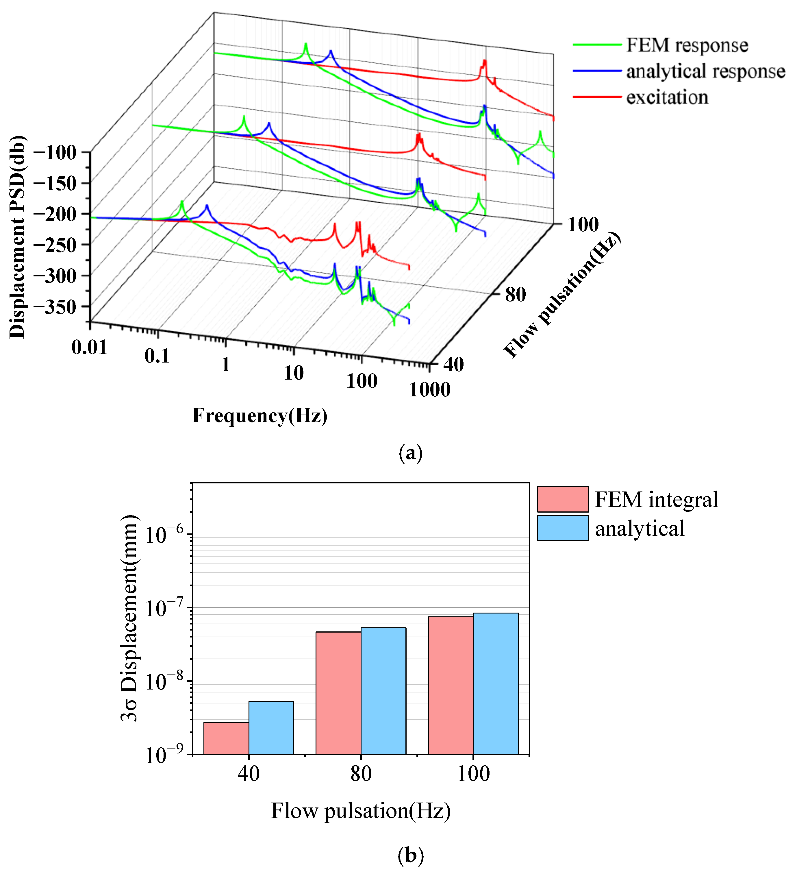
4.3. Vibration Isolation Performance Analysis

The primary purpose of applying the quasi-zero stiffness system to the DCM is to isolate vibrations from the crystal cooling system, preventing vibration interference with the core components of the DCM. In evaluating vibration isolation performance, key metrics include not only transmissibility but also 3σ displacement. In various practical application scenarios, vibration excitations exhibit randomness, with their amplitudes generally following a Gaussian distribution where higher amplitudes occur less frequently. The 3σ displacement refers to the maximum amplitude within the 3σ confidence interval of random vibration statistical data, with a confidence level of 99.737%. This implies that the probability of random vibration amplitudes being lower than the 3σ displacement is 99.737%.

In this section, using ANSYS Fluent, the vibration excitation of the cooling system under different flow pulsations is computed as the input to analyze the vibration isolation performance of the quasi-zero stiffness system. The finite element model shown in Figure 13 utilizes Static Structure, Modal, and Random Vibration solvers. Slightly differently from the previous chapters, firstly, the displacement boundary condition of the peripheral frame is removed from the simulation here because there is no need to examine the negative stiffness value for random vibration; secondly, spring 1 is removed, and the stiffness coefficient of spring 2 is modified to 25.3, which is more in line with the practical application scenarios. Lastly, to achieve quasi-zero stiffness, the dimensions of the LS are modified based on Equation (30) to a h = 0.3, l₀ = 70, b = 81, and u_x = 0.4.

The finite element simulation steps include compressing the LS through slider displacement, solving for the first 10 modal frequencies, and applying PSD excitation along the y-axis direction on the crystal surface for final solution completion.

The calculation formula for the PSD response (34) is as follows, where S_o represents the PSD response, S_i represents the PSD excitation, and H(ω) represents the frequency response function, which here equals the transmissibility function calculated by Equation (2).

$$S_o={\left(H\left(\omega \right)\right)}^2{S}_i$$

(34)

As shown in Figure 17a, the overall trend of the FEM and analytical curves is relatively consistent, significant vibration isolation at an excitation frequency of 1 Hz, and the PSD curve of the decibel is 10 lg. In the random vibration response, it can be seen that the peak of the natural frequency of the analytical and FEM curves at the very-low frequency has a small offset, which is caused by the computational error. The results at 100 Hz after the high-frequency region of the FEM are different from the analytical peak of the PSD. The reason for this is that the analytical calculated response PSD does not consider the frame modals, while the finite element simulation uses the modal superposition method to comprehensively calculate the effects of each order of modals, so the analytical value is bound to have a small error in the integral calculation of the 3σ displacement. The figure shows the results of the integral calculation using the PSD response output from the solver and the theoretically calculated PSD response; the displacements are very close and both are controlled on the nanometer scale. In addition, the very-high--frequency region of the simulated PSD curves shows a significant effect of the frame modal on the response amplitude, which indicates a possible error in the vibration isolation performance demonstrated by the theoretically calculated PSD curves in the very-high frequency region.

From Figure 17, it can be observed that, while the quasi-zero stiffness system exhibits effective isolation of high-frequency vibration excitations, like other isolation systems, it needs to avoid the bandwidth of strong energy in the excitation by adjusting its natural frequencies accordingly. The initial design step for a quasi-zero stiffness system is similar to other isolation systems: the first step is analyzing the excitation PSD data. Only after finding a suitable range of natural frequencies can the calculation of negative stiffness values begin.

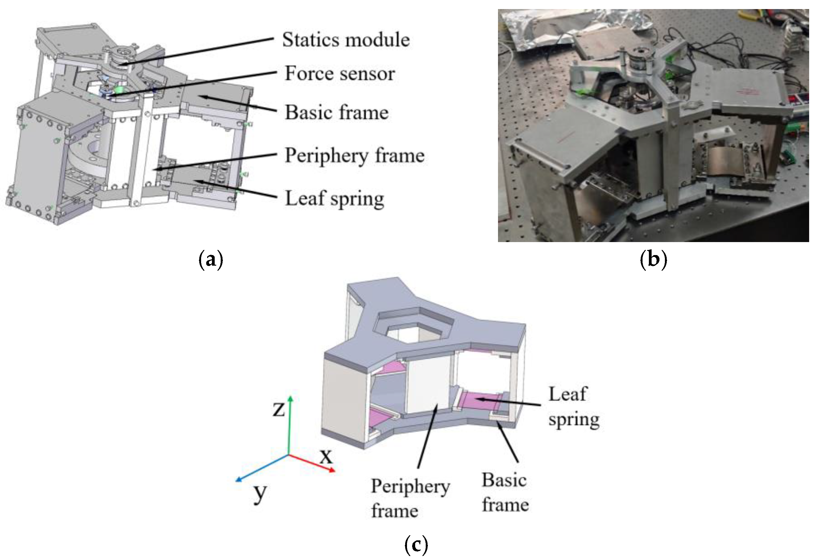
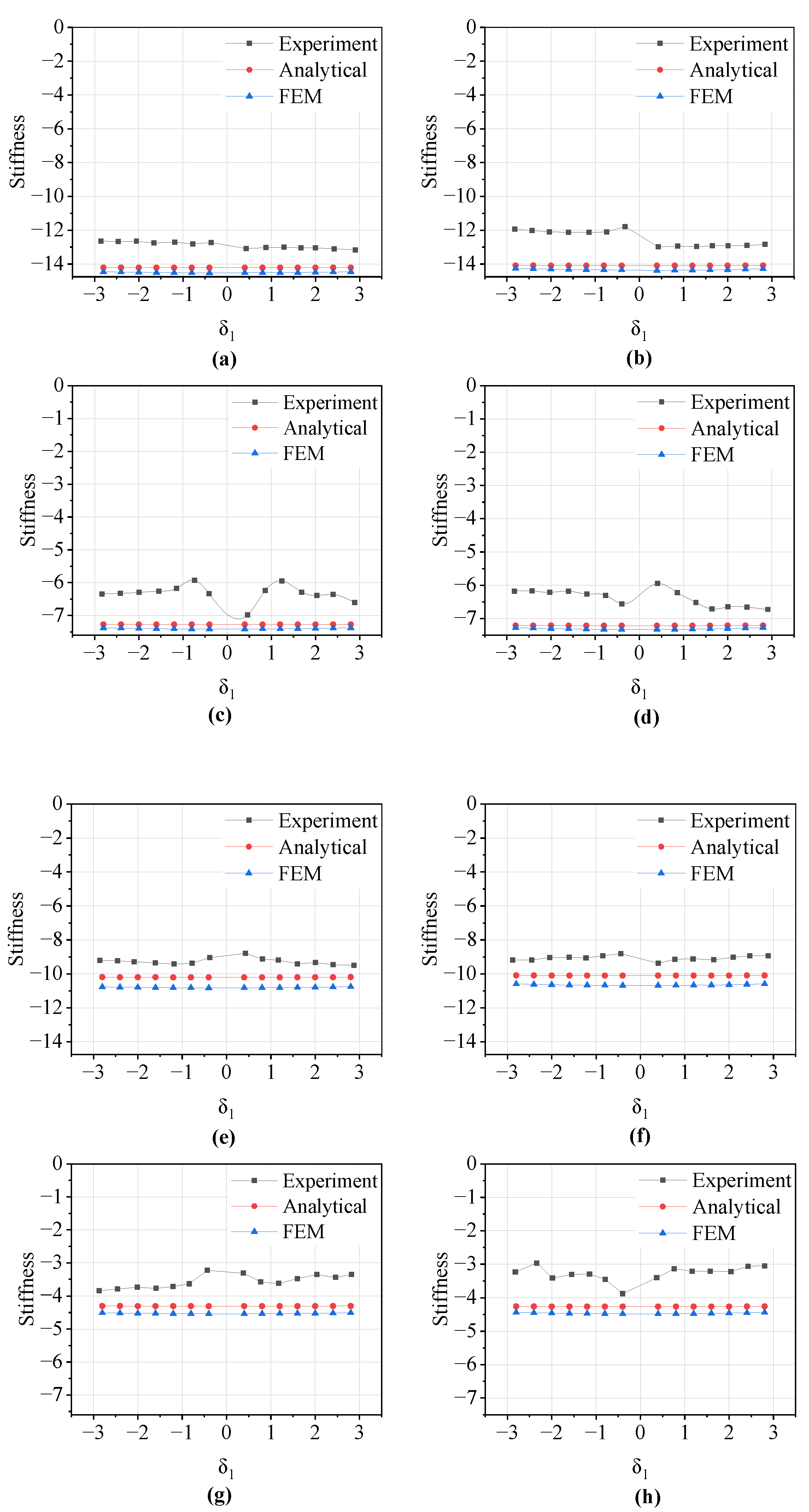
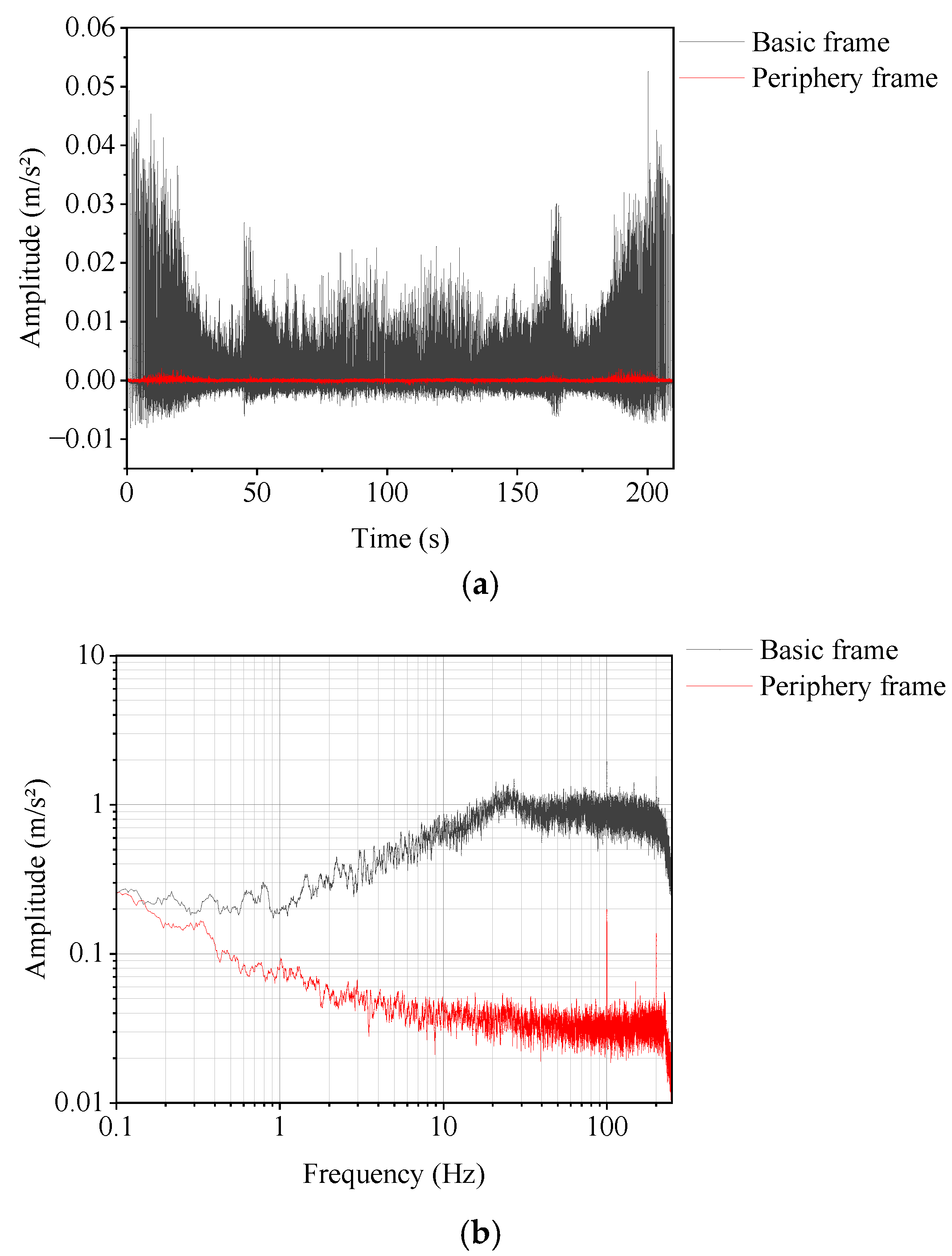
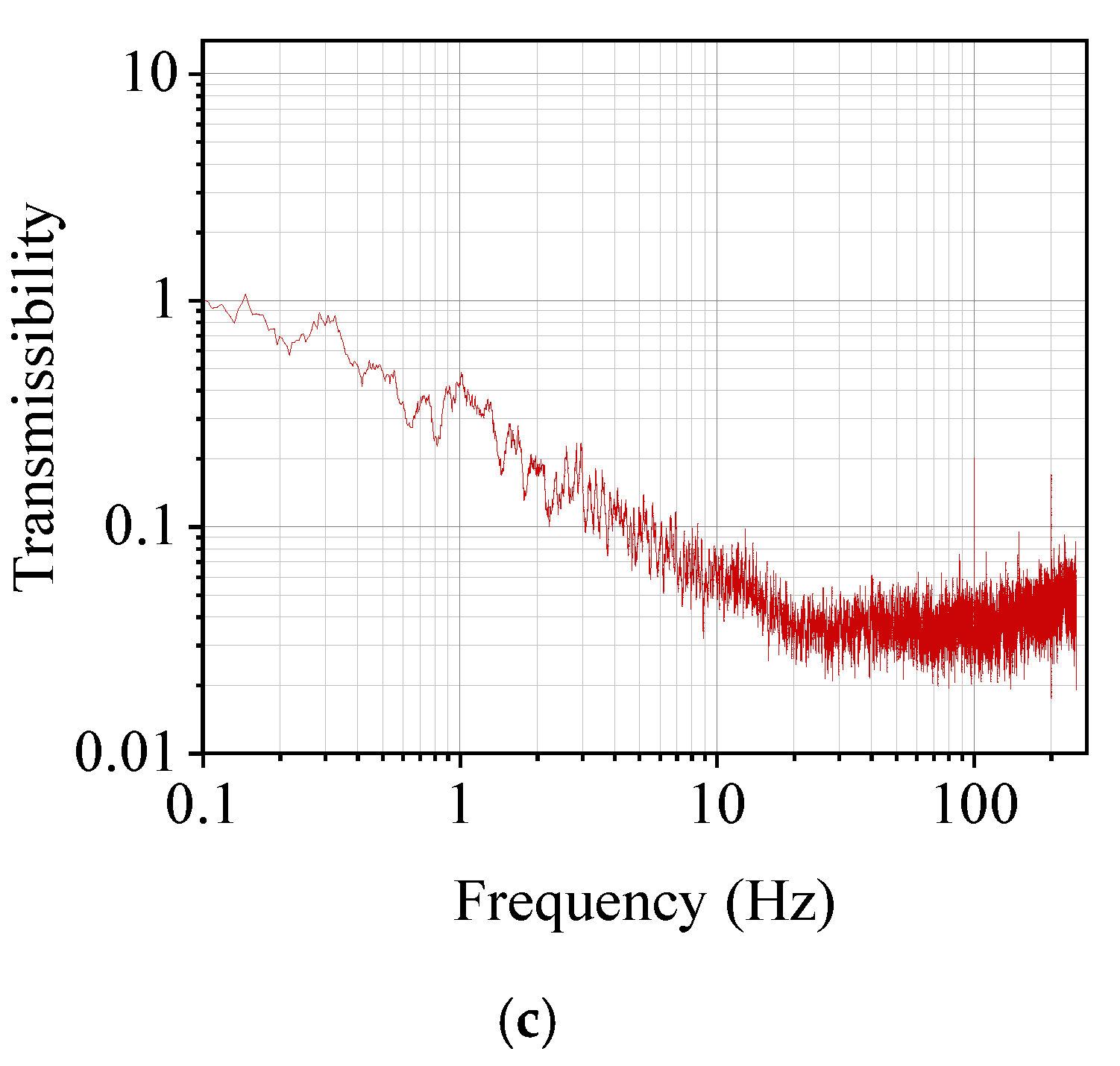
5. Experimental Verification

In the previous chapters, we have completed the derivation and finite element simulation verification of the formulas, in which the core theoretical results include the numerical calculation formula of the negative stiffness, the analytical solution of the compression load, and compression after compression buckling of the fixed beams at both ends, as well as the formula of the stress distribution on the surface of the negatively stiffened element. Due to the limitation of experimental conditions, we completed the verification of the negative stiffness formula. In addition, the analytical solution of the compression load and compression amount, as the most weighted item in the negative stiffness formula, can be indirectly verified by the experimental results to be accurate.

The experimental model is shown in Figure 18. In order to facilitate the processing and assembly, the experimental model is slightly different from the model in the previous chapters, but there is no change in the key components, such as coil springs and leaf springs. The experimental model used four sizes of leaf springs, respectively, for the static experiment, the experimental variables include thickness h, width b, length l₀, and compression u_x. The purpose of the static experiment is to measure the value of the negative stiffness; the experimental process is performed through the static module to drive the periphery frame along the vertical displacement; the purpose of the use of digital calipers and force transducers is to measure displacement and driving force, respectively, which will be used to obtain the overall stiffness coefficient. The negative stiffness is calculated by subtracting the stiffness coefficient of the coil spring from the overall stiffness coefficient, and the stiffness coefficient of the coil spring in this experimental model is about 16.5 N/mm.

While conducting the experiments, we have also completed the finite element simulation of this model, which is shown in Figure 18c, and the simulation process is consistent with the previous sections. The simulation results are also the stiffness coefficients of the negative stiffness element, which are compared with the theoretical calculations (the U_d term is omitted from the theoretical calculations; as mentioned in the previous sections, omitting the U_d term can save a lot of calculations, and, at the same time, it will not have a great influence on the accuracy), the experiments, and the finite element simulations.

As shown in Figure 19, the negative stiffness of the experimental results shows a more obvious change with displacement, which is mainly due to the fact that the static experiment used ordinary digital calipers for the measurement of displacement, and there is a certain deviation in their measurement accuracy. As a whole, most of the errors between experiments and theoretical calculations are less than 15%, while the errors between finite element simulation results and theoretical results are within 10%. Therefore, the calculation accuracy of Equation (30) for the negative stiffness can basically meet the actual needs of engineering, and the correction factor for the Ua term is also more accurate. It can be seen, in the figure, that the negative stiffness of the FEM is always lower than that of the analytical; this is because the value of the correction factor of (30) is conservative, which makes the negative stiffness effect of the analytical smaller compared to the FEM in order to prevent the negative stiffness effect from being stronger than the positive stiffness in the practical application. The experimental results are higher than the analytical and FEM results; this is probably because there are errors in both the FEM and analytical results, but the amount of error is small and within the acceptable range. The curves of theory and simulation seem to be basically kept constant; the reason for this is that the length of the leaf spring is much larger than the compression amount, and the frame displacement hardly affects its compression amount, so the negative stiffness value basically remains unchanged.

Each set of leaf springs is subjected to at least two experiments, and the data from multiple experiments need to be compared to confirm whether the overall stiffness and displacement curves are close, and, if there is a more similar result, the last measurement data are retained. Because the measuring tool is a digital caliper, there will be some errors in the measured values, resulting in fluctuations in the curves. The final data shown in Figure 19 focus on the overall stiffness and displacement curves during the comparison process and the local fluctuations are not dealt with for the time being. Therefore, the experimental data curve in the figure is the original data obtained from the measurement and has not been processed by other calculations.

In addition to the static experiments, we also verified the vibration isolation performance using the model. As shown in Figure 20, swept-frequency vibration experiments were carried out using a leaf spring with a b of 80, l₀ of 70, h of 0.25, and u_x of 0.4, and acceleration amplitudes were measured using an accelerometer for the basic and periphery frames, respectively. The signals in both the time and frequency domains indicate that the device has a significant vibration isolation effect. Due to the test equipment and environment, a more pronounced natural frequency was not obtained, but this does not affect the conclusion that the device has a vibration isolation effect. The reason may be that the vibration isolator filtered out too much vibration excitation, resulting in the response amplitude of the vibration-isolated part being too small to be measured. From the time domain signal, the response amplitude of the periphery frame is close to the noise amplitude. Because of the low signal-to-noise ratio of the signals, the frequency domain signals and the transfer rates demonstrated in Figure 20b,c were smoothed using a shifting smoothing process with a window width of 20, and the resolution of the spectra was 0.0047 Hz, so the smoothing process had no effect on the display of the natural frequencies. Figure 20b shows the presence of 100 Hz, 150 Hz, and 200 Hz peaks due to electromagnetic interference in the internal circuitry of the measuring instrument. The 50 Hz industrial frequency interference peaks were eliminated by grounding the sensor during the experiment, but the industrial frequency interference inside the instrument still exists.

6. Conclusions

Using a buckled LS fixed at both ends as a negative stiffness element can achieve a large negative stiffness. When combined with linear positive stiffness springs in a parallel arrangement, it forms a QZS system that effectively isolates low-frequency vibration excitations. In the calculation of negative stiffness values, the elastic potential energy generated by the elastic deformation of the LS and springs in both the horizontal and vertical directions is used to establish the force equilibrium equation of the quasi-zero stiffness system, obtaining an analytical solution for the negative stiffness value.

The accuracy of the negative stiffness value is verified using a finite element simulation. Static structural simulations are conducted to obtain the negative stiffness values of LSs with different lengths, widths, thicknesses, and compressions. By comparing data from 81 sets of finite element simulations with theoretical calculations, corrections are made to the analytical solution, significantly improving the accuracy of the negative stiffness values. Through the verification of experiments and finite element simulations, it was determined that the accuracy of the negative stiffness calculation formula is sufficient to meet the practical requirements. According to the dynamic deflection curve obtained during the derivation of the negative stiffness formula, the stress distribution of the compression buckling leaf springs in the form of fixed at both ends was deduced and verified by using finite element simulation, and the overall trend of the change is in line with the results of the analytical solution of the stress distribution in comparison with the value of the maximum stress. The simulation and experimental results demonstrate that the QZS system with flexural leaf spring structure has a certain vibration isolation performance, in which the random vibration simulation results show that the QZS isolation system significantly isolates the vibration excitation of the crystal cooling system. Therefore, the QZS system is suitable for the vibration isolation of ultra-high-stability DCM frames. It should be noted that QZS vibration isolation is a passive vibration isolation device, its dynamics are similar to those of traditional passive vibration isolation devices, and there are obvious characteristics of the natural frequency, so the design of quasi-zero stiffness vibration isolation needs to consider the vibration excitation characteristics of the application scenario, so that the natural frequency avoids the strong excitation energy frequency range.

References

1. Tsoutsouva, M.G.; Regula, G.; Ryningen, B.; Vullum, P.E.; Mangelinck-Noël, N.; Stokkan, G. Dynamic observation of dislocation evolution and interaction with twin boundaries in silicon crystal growth using in–situ synchrotron X-ray diffraction imaging. Acta Mater. 2021, 210, 116819. [Google Scholar] [CrossRef]
2. Li, A.; Gong, X.; Bai, Y.; Lu, Q.; Li, S.; Zhang, W.; Chai, K. Research on the Mechanism of Flow-Induced Vibration in the Cooling System of a Double Crystal Monochromator. Appl. Sci. 2024, 14, 2767. [Google Scholar] [CrossRef]
3. Soares, T.R.S.; Furtado, J.P.S.; de Albuquerque, G.S.; Saveri Silva, M.; Geraldes, R.R. Dynamical modelling validation and control development for the new High-Dynamic Double-Crystal Monochromator (HD-DCM-Lite) for Sirius/LNLS. In Proceedings of the 19th International Conference on Accelerator and Large Experimental Physics Control Systems (ICALEPCS 2023), Cape Town, South Africa, 7–13 October 2023. [Google Scholar]
4. Ciatto, G.; Chu, M.H.; Fontaine, P.; Aubert, N.; Renevier, H.; Deschanvres, J.L. SIRIUS: A new beamline for in situ X-ray diffraction and spectroscopy studies of advanced materials and nanostructures at the SOLEIL Synchrotron. Thin Solid Film. 2016, 617, 48–54. [Google Scholar] [CrossRef]
5. Shuo, C.; WanQian, Z.; ZhanFei, Z.; LiMin, Z.; Song, X. Research and optimization of flow-induced vibrations in a water-cooled monochromator. Rev. Sci. Instrum. 2024, 95, 035124. [Google Scholar]
6. Siming, G.; Dongjie, H.; Eryan, W.; Ruiqiang, S.; Pengyue, Z. Structure improvement and stability research of double crystal monochromator. Metrol. Sci. Technol. 2021, 65, 8–13. [Google Scholar]
7. Hiroshi, Y.; Yasuhisa, M.; Yasuhiro, S.; Ichiro, T.; Yuki, I.; Tomoyuki, T.; Masayuki, T.; Takanori, M.; Hikaru, K.; Yasunori, S.; et al. Challenges toward 50 nrad-stability of x-rays for a next generation light source by refinements of SPring-8 standard monochromator with cryo-cooled Si crystals. In AIP Conference Proceedings; AIP Publishing: Melville, NY, USA, 2019; Volume 2054. [Google Scholar]
8. Yichen, F.; Hongliang, Q.; Wanqian, Z.; Wenhong, J.; Yun, L.; Jie, W.; Zhongliang, L. Angular stability measurement of a cryocooled double-crystal monochromator at SSRF. Nucl. Instrum. Methods Phys. Res. Sect. A Accel. Spectrometers Detect. Assoc. Equip. 2020, 983, 164636. [Google Scholar]
9. Li, S. Analysis of foundation vibration pattern and coherence of Shanghai Light Source Experimental Hall. Noise Vib. Control. 2016, 36, 108–111+159. (In Chinese) [Google Scholar]
10. Ma, Z.; Rui, Z.; Yang, Q. Recent advances in quasi-zero stiffness vibration isolation systems: An overview and future possibilities. Machines 2022, 10, 813. [Google Scholar] [CrossRef]
11. Hamzehei, R.; Bodaghi, M.; Wu, N. Mastering the art of designing mechanical metamaterials with quasi-zero stiffness for passive vibration isolation: A review. Smart Mater. Struct. 2024, 33, 083001. [Google Scholar] [CrossRef]
12. Ge, Y.; Zhi-Yuan, W.; Xin-Sheng, W.; Sen, W.; Hong-Xiang, Z.; Lin-Chuan, Z.; Wen-Hao, Q.; Wen-Ming, Z. Nonlinear compensation method for quasi-zero stiffness vibration isolation. J. Sound Vib. 2022, 523, 116743. [Google Scholar]
13. Carrella, A.; Brennan, M.J.; Waters, T.P. Static analysis of a passive vibration isolator with quasi-zero-stiffness characteristic. J. Sound Vib. 2007, 301, 678–689. [Google Scholar] [CrossRef]
14. Carrella, A.; Brennan, M.J.; Kovacic, I.; Waters, T.P. On the force transmissibility of a vibration isolator with quasi-zero-stiffness. J. Sound Vib. 2009, 322, 707–717. [Google Scholar] [CrossRef]
15. Wei, Z.; Chun, C.; Ran, M.; Yan, H.; Weiping, W. Performance analysis of a quasi-zero stiffness vibration isolation system with scissor-like structures. Arch. Appl. Mech. 2021, 91, 117–133. [Google Scholar]
16. Wang, J.; Guo, Y. Multi-directional vibration isolation performances of a scissor-like structure with nonlinear hybrid spring stiffness. Nonlinear Dyn. 2024, 112, 8871–8888. [Google Scholar] [CrossRef]
17. Linchuan, G.; Axconny, K.; Rang-Lin, F.; Xu, W. Analysis of a passive scissor-like structure isolator with quasi-zero stiffness for a seating system vibration-isolation application. Int. J. Veh. Des. 2020, 82, 224–240. [Google Scholar]
18. Jiaxi, Z.; Xinlong, W.; Daolin, X.; Steve, B. Nonlinear dynamic characteristics of a quasi-zero stiffness vibration isolator with cam–roller–spring mechanisms. J. Sound Vib. 2015, 346, 53–69. [Google Scholar]
19. Song, Z.; Dayang, W.; Yongshan, Z.; Quantian, L. Design and testing of a parabolic cam-roller quasi-zero-stiffness vibration isolator. Int. J. Mech. Sci. 2022, 220, 107146. [Google Scholar]
20. Yonglei, Z.; Hao, W.; Haiyan, H.; Dongping, J. A novel quasi-zero stiffness isolator with designable stiffness using cam-roller-spring-rod mechanism. Acta Mech. Sin. 2025, 41, 524210. [Google Scholar]
21. Lian, X.; Deng, H.; Han, G.; Jiang, F.; Zhu, L.; Shao, M.; Liu, X.; Hu, R.; Gao, Y.; Ma, M.; et al. A low-frequency micro-vibration absorber based on a designable quasi-zero stiffness beam. Aerosp. Sci. Technol. 2023, 132, 108044. [Google Scholar]
22. Changqi, C.; Jiaxi, Z.; Linchao, W.; Kai, W.; Daolin, X.; Huajiang, O. Design and numerical validation of quasi-zero-stiffness metamaterials for very low-frequency band gaps. Compos. Struct. 2020, 236, 111862. [Google Scholar]
23. Zeyi, L.; Kai, W.; Tingting, C.; Li, C.; Daolin, X.; Jiaxi, Z. Temperature controlled quasi-zero-stiffness metamaterial beam for broad-range low-frequency band tuning. Int. J. Mech. Sci. 2023, 259, 108593. [Google Scholar]
24. Robertson, W.S.; Kidner, M.R.F.; Cazzolato, B.S.; Zander, A.C. Theoretical design parameters for a quasi-zero stiffness magnetic spring for vibration isolation. J. Sound Vib. 2009, 326, 88–103. [Google Scholar] [CrossRef]
25. Yang, W.; Yuanping, X.; Lu, Y.; Jin, Z.; Jarir, M.; Chaowu, J. An ultra-sensitive diamagnetic levitation accelerometer with quasi-zero-stiffness structure. Measurement 2025, 245, 116651. [Google Scholar]
26. Chaoran, L.; Yuewu, W.; Wei, Z.; Kaiping, Y.; Jia-Jia, M.; Huan, S. Nonlinear dynamics of a magnetic vibration isolator with higher-order stable quasi-zero-stiffness. Mech. Syst. Signal Process. 2024, 218, 111584. [Google Scholar]
27. Lei, X.; Xiang, S.; Li, C.; Xiang, Y. A 3D-printed quasi-zero-stiffness isolator for low-frequency vibration isolation: Modelling and experiments. J. Sound Vib. 2024, 577, 118308. [Google Scholar]
28. Xin, L.; Shuai, C.; Bing, W.; Xiaojun, T.; Liang, Y. A compact quasi-zero-stiffness mechanical metamaterial based on truncated conical shells. Int. J. Mech. Sci. 2024, 277, 109390. [Google Scholar]
29. Chunyu, Z.; Guangdong, S.; Yifeng, C.; Xiaobiao, S. A nonlinear low frequency quasi zero stiffness vibration isolator using double-arc flexible beams. Int. J. Mech. Sci. 2024, 276, 109378. [Google Scholar]
30. Haodong, Z.; Jiangjun, G.; Yao, C.; Zhengliang, S.; Hengzhu, L.; Pooya, S. A quasi-zero-stiffness vibration isolator inspired by Kresling origami. Structures 2024, 69, 107315. [Google Scholar]
31. Xiaolong, Z.; Xuhao, L.; Changcheng, L.; Ruilan, T.; Luqi, C.; Minghao, W. Design of hyperbolic quasi-zero stiffness metastructures coupled with nonlinear stiffness for low-frequency vibration isolation. Eng. Struct. 2024, 312, 118262. [Google Scholar]
32. Size, A.; Jianzheng, W.; Zhimin, X.; Huifeng, T. Analysis of negative stiffness structures with B-spline curved beams. Thin-Walled Struct. 2024, 195, 111418. [Google Scholar]
33. Changqi, C.; Xin, G.; Bo, Y.; Kai, W.; Yongsheng, Z.; Wei, Y.; Jiaxi, Z. Modelling and analysis of the quasi-zero-stiffness metamaterial cylindrical shell for low-frequency band gap. Appl. Math. Model. 2024, 135, 90–108. [Google Scholar]
34. Wu, Q.; Qiao, J.; Li, X.; Wang, S.; Li, B.; Wu, S.; Wang, Z.; Ji, J. NiTi Alloy Quasi-Zero Stiffness Vibration Isolation Structure with Adjustable Mechanical Properties. Machines 2025, 13, 92. [Google Scholar] [CrossRef]
35. Ji, L.; Yanhui, W.; Shaoqiong, Y.; Tongshuai, S.; Ming, Y.; Wendong, N. Customized quasi-zero-stiffness metamaterials for ultra-low frequency broadband vibration isolation. Int. J. Mech. Sci. 2024, 269, 108958. [Google Scholar]
36. Fossat, P.; Kothakota, M.; Ichchou, M.; Bareille, O. Dynamic bending model describing the generation of negative stiffness by buckled beams: Qualitative analysis and experimental verification. Appl. Sci. 2023, 13, 9458. [Google Scholar] [CrossRef]
37. Fulcher, B.A.; Shahan, D.W.; Haberman, M.R.; Conner Seepersad, C.; Wilson, P.S. Analytical and experimental investigation of buckled beams as negative stiffness elements for passive vibration and shock isolation systems. J. Vib. Acoust. 2014, 136, 031009. [Google Scholar] [CrossRef]
38. Geraldes, R.; Witvoet, G.; Vermeulen, J. The mechatronic architecture and design of the High-Dynamic Double-Crystal Monochromator for Sirius light source. Precis. Eng. 2022, 77, 110–126. [Google Scholar] [CrossRef]
39. Gere, J.M.; Goodno, B.J. Mechanics of Materials Translation; Machinery Industry Press: Norwalk, CT, USA, 2017; pp. 328–335, 710–761. (In Chinese) [Google Scholar]
Figure 1. Synchrotron radiation principle.
Applsci 15 03024 g001
Figure 2. (a) The compression buckling process commonly used in other similar studies; (b,c) the compression buckling process of the structure studied in this paper.
Applsci 15 03024 g002
Figure 3. (a) Bragg diffraction principle; (b) principle of DCM operation.
Applsci 15 03024 g003
Figure 4. DCM structure, the first crystal is mounted on the basic frame, the second crystal active adjustment mechanism is mounted on the peripheral frame, and the basic frame and the periphery frame are connected in the middle using a vibration isolation device.
Applsci 15 03024 g004
Figure 5. Frequency ratio and transmissibility.
Applsci 15 03024 g005
Figure 6. QZS vibration isolation system.
Applsci 15 03024 g006
Figure 7. Elastic potential energy in the QZS system.
Applsci 15 03024 g007
Figure 8. Compression buckling: (a) no-load state; (b) stable state, axial load F1 less than critical load, LS returns to initial position after removing external load F2; (c) unstable state, axial load F1 greater than critical load, LS remains in buckled state after removing external load F2; (d) boundary conditions and load forms for LS buckled.
Applsci 15 03024 g008
Figure 9. Theoretical calculation of compression displacement compared with finite element simulation. E of the LS is 193 GPa, b is 80 mm, and l0 is 70 mm.
Applsci 15 03024 g009
Figure 10. Buckling deflection curve of a beam with both ends fixed and one end eccentrically loaded.
Applsci 15 03024 g010
Figure 11. Comparison of finite element deflection curve and approximate deflection curve, with a l0 of 80 mm and a ux of 0.3 mm.
Applsci 15 03024 g011
Figure 12. Finite element simulation of negative stiffness values at different displacements, with a LS E of 193 GPa, b of 80 mm, l0 of 80 mm, h of 0.1 mm, ux of 0.1 mm, and N of 6.
Applsci 15 03024 g012
Figure 13. Finite element model: (a,b) boundary conditions and layout; (c) distribution of positive stiffness helical springs; (d) force reaction measurement locations.
Applsci 15 03024 g013
Figure 14. (a,c) LS with an h of 0.3 mm and ux of 0.3 mm; calculating the negative stiffness and transmissibility with different l0 and b; (b,d) LS with a b of 80 mm and l0 of 80 mm; calculating the negative stiffness and transmissibility with different h and ux; (e) LS with a b of 80 mm and l0 of 80 mm; separately calculating the force value of the Ua term with different h and ux.
Applsci 15 03024 g014aApplsci 15 03024 g014b
Figure 15. Comparison between the corrected theoretical values and the finite element results: (a) leaf spring with a b of 80 and a l0 of 80; calculated with different h and ux; (b) leaf spring with a h of 0.3 and a ux of 0.3; calculated with different b and l0.
Applsci 15 03024 g015
Figure 16. (a) Finite element simulation results for the 2D stress distribution of an LS with a l0 of 60, b of 20, h of 0.3, ux of 0.3, and δ1 = 1; (b) comparison between 1D stress distribution calculated for different l0 and the finite element simulation results for an LS with a h of 0.1, ux of 0.1, and δ1 = 1; (c) comparison between 1D stress distribution calculated for different l0 and the finite element simulation results for a leaf spring with a h of 0.3, ux of 0.3, and δ1 = 1.
Applsci 15 03024 g016
Figure 17. (a) Displacement PSD; (b) response 3σ displacement.
Applsci 15 03024 g017
Figure 18. Experimental model: (a) 3D model, (b) physical object, (c) FEM model.
Applsci 15 03024 g018
Figure 19. Comparison of results: (a) b = 80 l0 = 70 h = 0.25 ux = 0.6, (b) b = 80 l0 = 70 h = 0.25 ux = 0.4, (c) b = 80 l0 = 70 h = 0.2 ux = 0.6, (d) b = 80 l0 = 70 h = 0.2 ux = 0.4, (e) b = 70 l0 = 60 h = 0.2 ux = 0.6, (f) b = 70 l0 = 60 h = 0.2 ux = 0.4, (g) b = 70 l0 = 60 h = 0.15 ux = 0.6, (h) b = 70 l0 = 60 h = 0.15 ux = 0.4.
Applsci 15 03024 g019
Figure 20. Results of vibration isolation experiments: (a) time-domain signal, (b) Fourier transform of time-domain signal, (c) transmissibility.
Applsci 15 03024 g020aApplsci 15 03024 g020b