Enhancing Kidney Disease Diagnosis Using ACO-Based Feature Selection and Explainable AI Techniques

Abstract

Kidney disease is a global health concern, impacting a substantial part of the overall population and contributing to high morbidity and mortality rates. The initially diagnosed phases of kidney disease are often present without noticeable indications, leading to delayed diagnosis and treatment. Therefore, early detection is crucial to reducing complications and improving the lives of those impacted. However, the performance of previous automated approaches has often been hindered by suboptimal feature selection and algorithms’ “black-box” nature, which adversely affect their interpretability and clinical applicability. This paper aims to address these limitations by creating an effective machine-learning-based approach that integrates ant colony metaheuristic optimization algorithms for feature selection and explainable artificial intelligence techniques such as SHAP and LIME for model interpretation. The ant colony optimization method identified the most relevant feature subsets using a clinical dataset, reducing model complexity while preserving predictive accuracy. Performance evaluation shows that the extra trees classifier, when using optimized selected features, achieved the highest performance with an accuracy of 97.70% and an area under the curve of 99.55%, outperforming previous models trained on raw and complete processed feature sets. To enhance interpretability, the SHAP and LIME explainable techniques were employed, providing detailed insights into the contribution of key features such as TimeToEventMonths, HistoryDiabetes, and Age. This comprehensive framework, combining advanced feature selection with explainable models, improves clinical decision-making and fosters trust in machine learning applications for healthcare.

1. Introduction

Kidney disease (KD) significantly reduces the function of the kidneys in filtering waste and excessive fluid from the blood flow, resulting in severe health consequences. It is often associated with diabetes, hypertension, and glomerulonephritis, impacting millions of individuals and contributing to high morbidity and mortality rates worldwide [1,2,3]. KD often stays asymptomatic in its early stages, making it an undetected significant factor in mortality and increasing the risk of disease progression to advanced stages. Once KD reaches a critical stage, treatment options become limited, often requiring dialysis or kidney transplantation. Early diagnosis and intervention are crucial in preventing irreversible kidney damage.

Although traditional diagnostic techniques can confirm the existence of KD, they are ineffective in predicting its progression and response to treatment [4,5,6]. This limitation underscores the need for advanced predictive methodologies to improve early diagnosis and enhance clinical decision-making. Machine learning (ML) has gained significant attention for KD prediction because it analyzes complex clinical data and extracts meaningful patterns. The feature selection (FS) data preprocessing phase plays an important role in ML-based predictive models for KD. FS methods select optimal feature subsets while balancing relevance and are thus vital to improving classification accuracy. However, FS methods often involve significant challenges, such as determining optimal objective functions to guide the selection process, dealing with the computational complexity involved in evaluating feature subsets, and managing the trade-off between the number of selected features and the overall model performance.

With the vast number of possible feature subsets, the computational complexity of FS is high. It is an NP-hard combinatorial optimization problem. Exhaustive search methods are computationally infeasible, while traditional approaches such as finding an optimal characteristic set (FOCUS) often fail to produce satisfactory results. Metaheuristic algorithms, particularly those inspired by swarm intelligence and evolutionary strategies, have been introduced to tackle the problem. Although these algorithms show promising results in optimizing feature selection while balancing accuracy and computational efficiency [6,7], many suffer from stagnation in sub-optimal solutions, leading to reduced classification accuracy and subpar feature subset selection [8,9]. While contemporary optimizers such as the red fox optimizer, crayfish optimization algorithm, and reptile search algorithm have been introduced, no single optimization algorithm universally outperforms others across all problems (Wolpert’s no-free-lunch theorem) [10,11,12]. Therefore, an optimizer suitable for FS in KD prediction must be chosen to efficiently explore the search space, adapt dynamically to feature relevance, and avoid premature convergence.

This paper proposes an enhanced automated framework for KD prediction that integrates ant colony optimization (ACO) metaheuristic algorithms for feature selection to refine predictive accuracy while minimizing computational complexity. The AOC balances exploration and exploitation while effectively handling high-dimensional datasets [13]. Furthermore, eXplainable AI (XAI) techniques are incorporated to enhance model interpretability, making the predictions more transparent and clinically useful. Unlike conventional approaches, which often struggle with high computational overheads, the proposed framework efficiently identifies the most significant clinical features, balancing performance and interpretability. Key contributions of this paper are as follows:

• An optimized ACO-based feature selection approach is applied to extract the most relevant clinical features, reducing model complexity while maintaining high predictive accuracy.
• Multiple ML classifiers, including logistic regression (LR), random forest (RF), decision trees (DT), extreme gradient boosting (XGB), Adaboost, extra trees (ET), and k-nearest neighbors (KNN), are trained and evaluated for KD classification.
• The ET classifier achieves state-of-the-art performance using the ACO-selected features: an accuracy of 97.70% (outperforming the previous model by 4.41%), a precision of 97.15%, a recall of 98.37%, an F1-score of 97.73%, and an area under the curve (AUC) of 99.55%.
• The integration of XAI techniques such as SHAP and LIME to interpret model predictions bridges the gap between model accuracy and clinical applicability.

The remainder of this paper is structured as follows: Section 2 summarizes the previous research, and Section 3 provides background information related to the proposed method. Section 4 describes the proposed methodology, while Section 5 discusses the experimental results and analyses. Section 6 concludes the work.

2. Previous Research

Several ML-based solutions have recently been proposed for the prediction and detection of KD. In this section, previous research studies that utilize feature selection approaches are first reviewed, and then the relevant state-of-the-art techniques for KD prediction and detection are stated.

Feature selection techniques are divided into local and global categories. Global approaches identify the optimal features from the entire solution space, while local methods concentrate on the best features within a specific neighborhood of the feature space [14]. Metaheuristic algorithms are often used in both population-centric and neighborhood-centric optimization. Examples include genetic algorithms [15], ACO [16], binary gray wolf optimization [17], the butterfly optimization algorithm [18], particle swarm optimization (PSO) [19], etc. These algorithms effectively identify optimal feature subsets, balancing relevance and computational efficiency using global and local optimization methodologies [17]. A novel FS approach based on the firefly algorithm (FA) was proposed by [18] to reduce redundant features in high-dimensional medical datasets. The improved FA outperformed existing techniques in COVID-19 patient prediction by integrating genetic operators and quasi-reflexive-based learning. The hybrid nature of this approach demonstrates the potential of swarm intelligence in optimizing feature selection for medical disease diagnosis. A recent study [20] introduced a binary moth–flame optimization (B-MFO) approach for FS in medical datasets, addressing the limitations of existing binary metaheuristic algorithms. The study proposed three B-MFO variants using S-shaped, V-shaped, and U-shaped transfer functions to enhance scalability and effectiveness. Evaluated on seven medical datasets, B-MFO outperformed well-known binary metaheuristic algorithms in feature selection performance.

Some relevant state-of-the-art techniques for the prediction and detection of KD are as follows:

• Lambert et al. [15] proposed a hybrid classification framework for chronic kidney disease (CKD), utilizing ACO, GA, and PSO. The study showed that incorporating feature selection enhances classification performance, with ACO-FS outperforming GA-FS and PSO-FS when tested on a benchmark CKD dataset. LR was used as the final classifier, highlighting the effectiveness of FS methodologies in CKD prediction.
• Bilal et al. [17] introduced a novel CKD framework integrating binary gray wolf optimization (FS) and an extreme learning machine (ELM) for classification. The approach emphasizes the use of preprocessing techniques for handling missing values and optimizing data for deep analysis. Experimental results on a benchmark CKD dataset showed superior accuracy compared with existing models, highlighting the effectiveness of metaheuristic-driven FS in improving CKD diagnosis.
• Wibawa et al. [21] used a hybrid approach by combining k-nearest neighbors and Adaboost, and the correlation-based feature selection approach for selecting 17 features from 24, reaching a 98.1% accuracy. Similarly, Polat et al. [22] employed a support vector machine (SVM) classifier with a filter subset evaluator to select features. Thirteen significant characteristics were determined from a total of 24, and an accuracy of 98.5% was achieved. Aswathy et al. [23] presented a deep neural network (DNN) model using the flower pollination algorithm, which exhibited enhanced performance in various evaluation metrics. They processed the data and selected the key features using the oppositional crow search algorithm. They showed significant improvements over previous approaches by achieving a 98.75% accuracy. Although these models achieve high prediction accuracy, mainly by using feature selection techniques, they lack interpretability, which is essential for clinical adoption.
• Davide et al. [24] used ML approaches to predict KD progression in stages 3–5, using a feature ranking analysis to find the most important clinical parameters driving disease development. The study focused on feature ranking, achieving a good competitive accuracy of 84.3%. Wickramasinghe et al. [25] focused on collecting information from patient medical records to develop a framework that provides personalized dietary plans for KD patients.
• Ghosh et al. [26] proposed a ML-based approach for chronic KD prediction, employing clinical, laboratory, and demographic features. Among the five models, XGBoost achieved the highest accuracy (93.29%) and AUC (0.9689). Further interpretation using XAI techniques, namely SHAP and LIME, highlighted the importance of features like creatinine, HgbA1C, and age, enhancing the model interpretability for clinicians.

The above studies collectively demonstrate the potential of ML techniques to improve the accuracy of KD diagnosis and prediction; further details can be seen in

Table 1. Summary of previous research approaches to diagnosing KD.

Ref.	Problem	Objective	Contribution	Experimental Results
[21]	KD symptoms are non-specific, making diagnosis challenging.	To improve KD diagnosis quality using feature selection methods.	Developed an ensemble model using Adaboost and CFS with various classifiers.	Achieved highest performance with KNN, CFS, and Adaboost.
[22]	Early KD detection is required due to slow disease progression.	To improve SVM classification of KD using FS methods.	Applied wrapper and filter approaches with SVM.	Best performance achieved with a filtered subset evaluator.
[23]	IoT-based data analysis to manage high mortality.	To build an IoT-based KD diagnosis model for high performance.	Proposed FPA-DNN using the flower pollination algorithm for DNN parameter tuning.	The proposed approach achieved good experimental results.
[25]	Identifying diet plans for KD patients.	Classification of diet plans for KD patients.	Developed dietary prediction models based on potassium levels.	Multiclass decision forest achieved the highest performance
[26]	Chronic KD prediction using clinical and geographical data.	Classification of KD patients and interpretation using XAI.	Developed an interpretable ML framework for classifying KD patients.	Achieved good results and interpretation analysis of features.

. However, many existing models need more interpretability, which is essential for clinical adoption. The current study addresses this gap by integrating XAI techniques to enhance the transparency of ML models, thereby aiding in the clinical decision-making process.

3. Background Information

This section provides background information for the development of the proposed KD prediction system. It encompasses machine learning classifiers, the ACO optimization method, XAI methods, and performance evaluation metrics. These components underpin the advancement and efficacy of the automated diagnostic system.

3.1. Machine Learning Algorithms

In the medical field, ML algorithms are often used for clinical decision support and predictive analytics to help diagnose various diseases, including KD. Several previous research studies employed ML approaches for KD prediction. Frequently used algorithms include logistic regression, Adaboost, random forest, decision trees, extra gradient boosting, extra trees, and k-nearest neighbor classifiers [4,5,22,27,28].

In this paper, the extra trees (ET) classifier showed the best accuracy when used with ACO-selected features. The ET classifier is an ensemble learning technique widely used for classification tasks. It builds multiple decision trees by randomly selecting features and splitting points. This randomness often helps reduce overfitting and improves model generalization. ET is computationally efficient due to its simplified construction process. It has been shown to perform well with large datasets and high-dimensional features, making it suitable for complex medical datasets. Its robust handling of noisy data and ability to capture intricate relationships make it a preferred choice in many clinical decision-support systems.

3.2. Ant Colony Optimization Algorithm

ACO is a metaheuristic algorithm that draws inspiration from ants’ foraging habits. In ACO, artificial ants replicate the behavior of actual ants in finding food by creating pathways between their colony and the food supply while leaving pheromone trails along the way. Pheromone trails diminish over time but are reinforced through frequent usage by ants, increasing the likelihood that extensively used pathways will be selected by additional ants [29]. ACO is extensively used to address complex optimization challenges across several domains.

In the context of feature selection, ACO adapts ant behavior to identify the most relevant subset of features from a specified dataset [30]. In this scenario, features are shown as nodes in a graph (G), with ants starting their journey from random features. Each ant probabilistically selects features for inclusion in the subset based on pheromone levels and heuristic information, which indicate the quality of the features relevant to the problem being tackled.

The probability ${\mathrm{P}}_{\mathrm{i}}^{\mathrm{k}}\left(\mathrm{t}\right)$ of ant k selecting feature i at time t is determined using the following Equation (1):

$${\mathrm{P}}_{\mathrm{i}}^{\mathrm{k}}\left(\mathrm{t}\right)=\{{\displaystyle \frac{\left[{\mathsf{\tau }}_{\mathrm{i}}\right]{[\mathsf{\mu }}_{\mathrm{i}}{]}^{\mathsf{\beta }}}{{\sum }_{\mathrm{u}\in {\mathrm{N}}_{\mathrm{i}}}\left[{\mathsf{\tau }}_{\mathrm{i}}\right]{[\mathsf{\mu }}_{\mathrm{i}}{]}^{\mathsf{\beta }}}}\}$$

(1)

where ${\mathsf{\tau }}_{\mathrm{i}}$ represents the pheromone level of feature i, ${\mathsf{\mu }}_{\mathrm{i}}$ is the heuristic information (e.g., feature relevance), and $\mathsf{\beta }$ controls the relative importance of pheromone versus heuristic information. Ants move across features based on these probabilities, reinforcing successful paths as they explore the feature space.

Once all the ants complete their traversal, a global pheromone update occurs, which adjusts the pheromone levels of features based on their contribution to the solution. The pheromone update rule is given by Equation (2):

$${\mathsf{\tau }}_{\mathrm{j}}\left(\mathrm{t}+1\right)=\left(1-\mathsf{\rho }\right){\mathsf{\tau }}_{\mathrm{j}}\left(\mathrm{t}\right)+∆{\mathsf{\tau }}_{\mathrm{j}}$$

(2)

Here, $\mathsf{\rho }$ is the pheromone decay parameter, and $∆{\mathsf{\tau }}_{\mathrm{j}}$ represents the pheromone reinforcement for feature j, reflecting the effectiveness of features. This iterative process of probabilistic selection, pheromone update, and reinforcement allows ACO to converge on an optimal or near-optimal set of features, improving the performance of ML models while reducing dimensionality.

3.3. EXplainable Artificial Intelligence (XAI)

XAI aims to mitigate ML models’ “black box” characteristics by offering intelligible explanations for their decision-making methods. SHAP and LIME are two of the most popular XAI techniques.

3.3.1. The SHAP Explanation Method

Lundberg and Lee presented the SHapley Additive exPlanations (SHAP) approach in 2017 [31]. This approach uses game theory concepts to explain model predictions locally. In this framework, the model functions as the game regulations, while the input features act as individuals. Observed features participate, while unobserved features abstain.

SHAP computes Shapley values by assessing the predictive model using various feature combinations and estimating the average difference in prediction when a feature is included instead of when it is removed. This variant shows how the feature impacts the model’s prediction for a given input, yielding numerical Shapley values that measure each feature’s contribution. SHAP derives these values by combining linear equations with binary variables to determine whether a particular feature is functional [32].

The SHAP approach can be summarized as follows: A pre-trained model, $\mathrm{f}$ SHAP, approximates a more interpretable model, g, for a given input vector [${\mathrm{x}}_1,{\mathrm{x}}_2,\dots ,{\mathrm{x}}_{\mathrm{p}}$] of $p$ features. This model emphasizes the contribution of particular features to total predictions of overall potential feature subsets. The following formula in Equation (3) defines the representation of the model g:

$$\mathrm{g}\left(\mathrm{z}\right)={\mathrm{\varnothing }}_0+\sum _{i=1}^M{\mathrm{\varnothing }}_{\mathrm{i}}{\mathrm{z}}_{\mathrm{i}}$$

(3)

where ${\mathrm{\varnothing }}_0$ represents the model’s baseline value (the mean output), and [${\mathrm{z}}_1,{\mathrm{z}}_2,\dots ,{\mathrm{z}}_{\mathrm{p}}$] is a refined representation of the input x, with (${\mathrm{z}}_{\mathrm{i}}$ = 1) indicating if the feature contributes to the prediction and 0 if it does not. The coefficient i∈R represents the Shapley value of each feature and a weighted average of the contributions from every feature combination. The size of each combination determines the weights.

Specifically, the following Equation (4) is used to determine ${\mathrm{\varnothing }}_{\mathrm{i}}$:

$${\mathrm{\varnothing }}_{\mathrm{i}}\left(\mathrm{f},\mathrm{x}\right)=\sum _{\mathrm{z}\le {\mathrm{x}}^{\prime }}{\displaystyle \frac{\left|\mathrm{z}\right|!\left(\mathrm{p}-\left|\mathrm{z}\right|-1\right)!}{\mathrm{p}!}}[{\mathrm{f}}_{\mathrm{x}}\left(\mathrm{z}\right)-{\mathrm{f}}_{\mathrm{x}}({\displaystyle \raisebox{1ex}{$\mathrm{z}$}\!\left/ \!\raisebox{-1ex}{$\mathrm{i}$}\right.})]$$

(4)

In this context, ${\varnothing }_i$ represents the Shapley value for feature $\mathrm{i}$, $\mathrm{f}$ is the model, $\mathrm{x}$ is the input data point, and ${\mathrm{x}}^{\prime }$ refers to the distilled data input. The term $\left|\mathrm{z}\right|$ denotes the count of non-zero elements in $\mathrm{z}$, and the $\mathrm{z}$ subset $x^{\prime }$ includes all z vectors with non-zero components aligning with those in ${\mathrm{x}}^{\prime }$. The expression ${\mathrm{f}}_{\mathrm{x}}\left(\mathrm{z}\right)-{\mathrm{f}}_{\mathrm{x}}\left({\displaystyle \raisebox{1ex}{$\mathrm{z}$}\!\left/ \!\raisebox{-1ex}{$\mathrm{i}$}\right.}\right)$ indicates the contribution of the $\mathrm{i}$th variable to the prediction.

SHAP yields a set of feature weights that provide insights into the model’s predictions, accounting for interactions among features and offering a comprehensive understanding of the model’s behavior. While calculating Shapley values for all possible feature combinations is computationally intensive, SHAP can be efficiently implemented for models with tree-like structures.

3.3.2. LIME Explanation Method

LIME, an acronym for “Local Interpretable Model-agnostic Explanations”, is a technique intended to clarify the connection between the outputs of a pre-trained model and its input parameters, whatever the model’s underlying structure may be. LIME uses a subset of the original data centered on the instance of interest to train a more simple, interpretable model, usually a linear model, which approximates the behavior of complicated models close to specific data points [33]. This subset is generated by adjusting the instance’s attributes while keeping the label unchanged. Examining the simpler model’s performance with these altered samples might give insights into the behavior of the original model.

The mathematical representation of LIME’s explanations for a certain observation $x$ is shown in Equation (5):

$$\mathrm{\varnothing }\left(\mathrm{x}\right)={\mathrm{a}\mathrm{r}\mathrm{g}\mathrm{m}\mathrm{i}\mathrm{n}}_{\mathrm{g}\in \mathrm{G}}\mathrm{L}\left(\mathrm{f},\mathrm{g},{\mathsf{\pi }}_{\mathrm{x}}\right)+\mathrm{\Omega }\left(\mathrm{g}\right)$$

(5)

In this Equation, $\mathrm{G}$ signifies the collection of interpretable models, whereas $\mathrm{g}\in \mathrm{G}$ specifies the explanatory model. The function f translates from ${\mathrm{R}}^{\mathrm{d}} \text{to} \mathrm{R}$, and the closeness estimate between an instance z and x is denoted by ${\mathsf{\pi }}_{\mathrm{x}}\left(\mathrm{z}\right)$. The complexity of g is represented by $\mathrm{\Omega }\left(\mathrm{g}\right)$. LIME emphasizes its model-agnostic feature by minimizing the loss function L without taking on any particular form for f. The magnitude of $\mathrm{L}$ signifies the accuracy of the estimation, indicating the extent to which g represents f inside the domain specified by $\mathrm{\varnothing }\left(\mathrm{x}\right)$.

The LIME procedure usually involves the following steps: (1) identify the precise data points requiring understanding for the algorithm’s predictions; (2) generate novel data points by independently affecting the attributes of the chosen instance while preserving the label constant; (3) employ the complex black-box model to predict outcomes for each altered data point and document the appropriate input features; (4) train an interpretable model, such as linear regression or decision tree, utilizing the input variables as inputs and target values; and (5) analyze the coefficients from the interpretable model to ascertain which features substantially impact the prediction for the specified instance.

The main advantage of LIME is its model-agnostic characteristic, which enables it to interpret many classifiers, such as decision trees and neural networks. However, it is essential to recognize that LIME provides localized explanations for specific predictions and may only partly reflect the overall behavior of the model.

3.4. Performance Evaluation Metrics

Several performance evaluation metrics detailed in Equations (6)–(10) were used to evaluate the model’s performance, including the accuracy, area under the AUC, precision, recall, and F1-score. Kappa and MCC metric equations can be found in the study by [34]. The metrics rely on four components: true positives (TP), true negatives (TN), false positives (FP), and false negatives (FN), which represent instances accurately identified as positive, accurately identified as negative, inaccurately identified as positive, and inaccurately identified as negative, respectively.

$$\mathrm{A}\mathrm{c}\mathrm{c}\mathrm{u}\mathrm{r}\mathrm{a}\mathrm{c}\mathrm{y}={\displaystyle \frac{\mathrm{T}\mathrm{P}+\mathrm{T}\mathrm{N}}{\mathrm{T}\mathrm{P}+\mathrm{T}\mathrm{N}+\mathrm{F}\mathrm{P}+\mathrm{F}\mathrm{N}}}$$

(6)

$$\mathrm{P}\mathrm{r}\mathrm{e}\mathrm{c}\mathrm{i}\mathrm{s}\mathrm{s}\mathrm{i}\mathrm{o}\mathrm{n}={\displaystyle \frac{\mathrm{T}\mathrm{P}}{\mathrm{T}\mathrm{P}+\mathrm{F}\mathrm{P}}}$$

(7)

$$\mathrm{R}\mathrm{e}\mathrm{c}\mathrm{a}\mathrm{l}\mathrm{l}={\displaystyle \frac{\mathrm{T}\mathrm{P}}{\mathrm{T}\mathrm{P}+\mathrm{F}\mathrm{N}}}$$

(8)

$$\mathrm{A}\mathrm{U}\mathrm{C}=\int \left(\mathrm{T}\mathrm{P}\mathrm{R}\right)\mathrm{d}\left(\mathrm{F}\mathrm{P}\mathrm{R}\right)$$

(9)

$$\mathrm{F}1-\mathrm{s}\mathrm{c}\mathrm{o}\mathrm{r}\mathrm{e}=2\left({\displaystyle \frac{\mathrm{P}\ast \mathrm{R}}{\mathrm{P}+\mathrm{R}}}\right)$$

(10)

4. Methodology

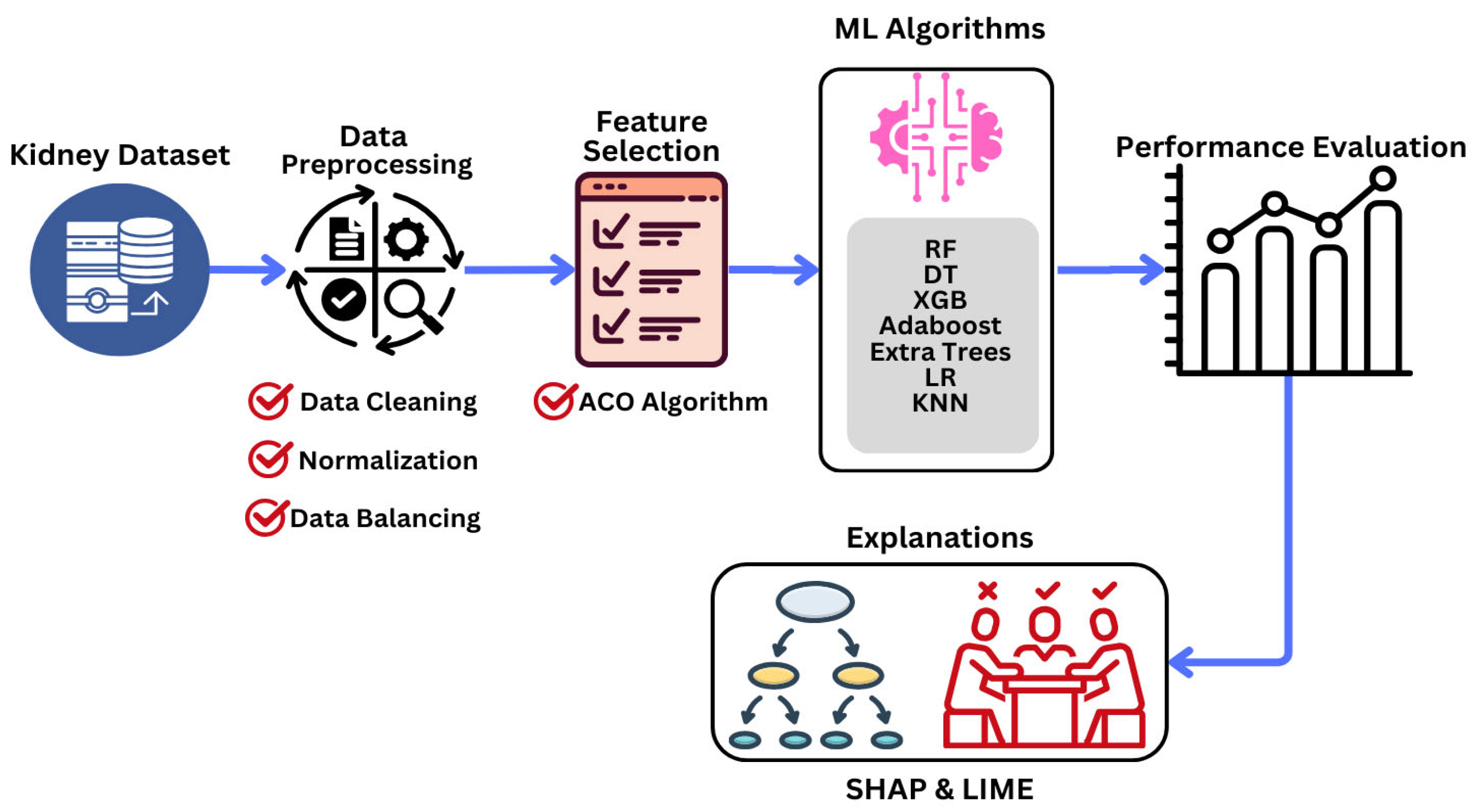
Figure 1 outlines the proposed interpretable ML technique for KD prediction. It consists of data collection and preprocessing stages, FS, classification, and the employment of ML algorithms and XAI methodologies to provide local and global explanations. First, a clinical KD dataset with essential characteristics is chosen and preprocessed. In the FS stage, the ACO FS approach is used to identify the most important features by calculating their importance scores. These features are subsequently used for the classification of ML algorithms. Several ML classifiers are trained and tested on the chosen subset, whose performance is evaluated using various metrics. In the last stage, the SHAP and LIME methodologies thoroughly evaluate their accuracy and interpretability. In the following subsections, the stages are explained in detail.

4.1. Data Description and Preprocessing

The public clinical data used in this research was obtained from Tawam Hospital in Abu Dhabi between January and December 2018 [35] (https://figshare.com/articles/dataset/6711155?file=12242270 (accessed on 1 September 2024)). The original dataset included information for 544 patients. However, only the data of 491 patients were considered, eliminating those who were missing baseline serum HgbA1C data [35]. The dataset consists of clinical, social, and physiological information on KD patients, with key factors such as gender, age, history of vascular, hypertension, dyslipidemia medication, smoking, and hypertension (HTN), among many other factors.

Categorical features include gender and medical history attributes (e.g., diabetes, coronary heart disease, vascular disease, smoking, hypertension, dyslipidemia, obesity, etc.), denoted using binary values (0, 1). The target variable is a binary classification of KD-Yes and KD-No.

Table 2. KD dataset features (STD: standard deviation).

No.	Features	Type	Description	Mean	Median	STD
1	Gender	String	Sex, either male or female
2	AgeBaseline	Numbers	Age in years	53.20	54	13.82
3	HistoryDiabetes	Binary	Patient with or without diabetes
4	HistoryCHD	Binary	Coronary heart disease (yes, no)
5	HistoryVascular	Binary	With or without vascular disease
6	HistorySmoking	Binary	Patient with or without smoking
7	HistoryHTN	Binary	History of hypertension
8	HistoryDLD	Binary	Patient with or without dyslipidemia
9	HistoryObesity	Binary	Patient with or without obesity
10	DLDmeds	Binary	Dyslipidemia medication
11	DMmeds	Binary	Diabetes medication
12	HTNmeds	Binary	Hypertension medication
13	ACEIARB	Binary	History of ACEIARB use
14	CholesterolBaseline	Numeric	Cholesterol	4.97	5	1.09
15	TriglyceridesBaseline	Numeric	Triglycerides	1.31	1.11	0.79
16	HgbA1C	Numeric	Glycosylated hemoglobin type AIC	6.59	6.10	1.71
17	CreatinineBaseline	Numeric	Creatinine	67.85	66	17.91
18	eGFRBaseline	Numeric	Glomerular filtration rate	98.11	98.05	18.50
19	sBPBaseline	Numeric	Systolic blood pressure	131.37	131	15.69
20	dBPBaseline	Numeric	Diastolic blood pressure	76.87	77	10.71
21	BMIBaseline	Numeric	Body mass index	30.18	29.57	6.20
22	TimeToEventMonths	Numbers	Time information of events in months	83.06	93	26.01
23	EventKD35	Binary	Patient with KD-Yes or KD-No

shows a comprehensive overview of these features according to their primary outcome.

Some steps were incorporated into the data preprocessing stage to ensure that the dataset was suitable for ML analysis. Initially, the dataset was cleaned, and missing values were handled using iterative imputation. Continuous variables were imputed with the mean, and categorical variables were imputed with the most common value according to the criteria in [36].

Normalization was performed using min–max scaling to rescale categorical and continuous variables, guaranteeing consistency across features. This procedure mitigated potential bias generated by differences in measurement scales and distribution ranges, as shown in the normalization method in Equation (11). This approach makes correct model interpretation quicker and enhances performance.

$${\mathrm{x}}_{\mathrm{n}\mathrm{o}\mathrm{r}\mathrm{m}\mathrm{a}\mathrm{l}\mathrm{i}\mathrm{z}\mathrm{e}\mathrm{s}}={\displaystyle \frac{\mathrm{x}-\mathrm{m}\mathrm{i}\mathrm{n}\left(\mathrm{X}\right)}{\max \left(\mathrm{X}\right)-\mathrm{m}\mathrm{i}\mathrm{n}\left(\mathrm{X}\right)}}$$

(11)

Initially, there was a significant class imbalance in the dataset, with 56 KD-Yes instances (11.41%) out of 491 patients. To address this imbalance, the synthetic minority over-sampling method (SMOTE) was used, which generated synthetic samples for the minority class until KD-Yes and KD-No had 435 occurrences each, resulting in a 1:1 ratio. SMOTE uses the k-nearest neighbors (KNN) approach to create new instances of the minority class, ensuring that synthetic samples retain significant feature distributions rather than simple replication.

To evaluate the influence of SMOTE, we evaluated the model performance before and after resampling using multiple evaluation metrics. Experimental results indicated that the minority class was more effectively detected, without a substantial risk of overfitting, based on the KD-Yes cases (see Section 5 for detailed experimental results). SMOTE maintains overall classification performance while balancing the dataset and improving the model’s capacity to predict KD-Yes instances.

4.2. Feature Selection and ML Classification

In the context of KD prediction, intelligently identifying the most informative features from the processed training data is crucial. This approach employs the ACO metaheuristic algorithm to extract key clinical features from the processed data. As explained in Section 3.2, the processed data is input into the ACO method, and the evaluation function assigns an importance score to each feature. Subsequently, the top-k thresholding method outlined in [28] is applied to identify the most significant features based on their importance scores. This method ranks features in descending order according to their importance scores derived from feature selection techniques. The top k features are then selected to form a refined subset, which is subsequently used to build a predictive model to enhance accuracy and computational efficiency. These selected features are then used for training ML classifiers, as illustrated in Figure 2.

During the classification phase, multiple ML algorithms are trained and evaluated using the feature subset selected by ACO. Each classifier is trained using an 80:20 training–validation split, and its performance is optimized through k-fold cross-validation. The classifier achieving the highest performance is selected as the optimal model.

4.3. Interpretation Phase

Finally, the interpretation phase integrates XAI techniques, specifically SHAP and LIME. These methods analyze the influence of individual features on model predictions at both local and global levels, providing meaningful insights into the model’s decision-making process.

Algorithm 1 below schematically shows the overall approach for the proposed interpretable KD prediction framework. It presents a structured pipeline for feature selection and classification, seamlessly combining optimization, evaluation, and interpretability to enhance the predictive accuracy and explainability of KD diagnosis models.

Algorithm 1 Interpretable KD Prediction Model
Input: Preprocessed KD dataset D, Number of selected features k, $\text{Classifier set} {\left\{{\mathrm{C}}_{\mathrm{i}}\right\}}_{\mathrm{i}=1}^{\mathrm{n}}$ Output: $\text{Best-performing classifier model} {\mathrm{C}}^{\prime }$, Interpretable explanations
1:	Step 1: Data Preprocessing
2:	Normalize dataset D using min–max scaling:
3:		${\mathrm{D}}^{\prime }={\displaystyle \frac{\mathrm{D}-{\mathrm{D}}_{\mathrm{m}\mathrm{i}\mathrm{n}}}{{\mathrm{D}}_{\mathrm{m}\mathrm{a}\mathrm{x}}-{\mathrm{D}}_{\mathrm{m}\mathrm{i}\mathrm{n}}}}$
4:	$\text{Balance classes in} {\mathrm{D}}^{\prime }$ to address class imbalance using SMOTE.
5:	Step 2: Feature Selection using ACO
6:	$\text{Initialize ant colony optimization parameters: population} \mathrm{P}, \text{iterations} \mathrm{T}, \text{evaporation rate} \mathsf{\rho }$.
7:	$\text{Calculate the importance score} \mathrm{S}\left({\mathrm{f}}_{\mathrm{i}}\right)$$\text{for each feature} {\mathrm{f}}_{\mathrm{i}}\in \mathrm{F}$.
8:	$\text{Update pheromone} {\mathsf{\tau }}_{\mathrm{i}\mathrm{j}}$$\text{for feature subsets} {\mathrm{F}}_{\mathrm{t}}$ based on scores:
9:		${\mathsf{\tau }}_{\mathrm{i}\mathrm{j}}=\left(1-\mathsf{\rho }\right).{\mathsf{\tau }}_{\mathrm{i}\mathrm{j}}+\mathsf{\rho }.\mathrm{S}\left({\mathrm{f}}_{\mathrm{i}}\right)$
10:	$\text{Select subset} {\mathrm{F}}_{\mathrm{k}}$$\text{containing the top} \mathrm{k} \text{features with the highest} \mathrm{S}\left({\mathrm{f}}_{\mathrm{i}}\right)$:
11:		${\mathrm{F}}_{\mathrm{k}}=\mathrm{t}\mathrm{o}\mathrm{p}-\mathrm{k}(\mathrm{F},\mathrm{S})$
12:	Step 3: Classifier Training and Evaluation
13:	$\text{For each classifier} {\mathrm{C}}_{\mathrm{i}}\in ({\mathrm{C}}_1,{\mathrm{C}}_2,\dots ,{\mathrm{C}}_{\mathrm{n}})$
14:		$\text{Train} {\mathrm{C}}_{\mathrm{i}}$$\text{on} {\mathrm{F}}_{\mathrm{k}}$ using an 80:20 training–testing split.
15:		Perform k-fold cross-validation to optimize performance metrics M (e.g., accuracy, precision, recall, F1-score, Kappa, MCC):
		${\mathrm{M}}_{\mathrm{i}}$$=\mathrm{evaluate}({\mathrm{C}}_{\mathrm{i}}$$,{\mathrm{F}}_{\mathrm{k}}$)
16:	$\text{Select} {\mathrm{C}}^{\prime }=\mathrm{a}\mathrm{r}\mathrm{g}{\mathrm{m}\mathrm{a}\mathrm{x}}_{{\mathrm{C}}^{\prime }}{\mathrm{M}}_{\mathrm{i}}$
17:	Step 4: Explainability Analysis using SHAP and LIME
18:	Initialize SHAP and LIME explainers.
19:	$\text{For each instance} \mathrm{x} \mathrm{in} {\mathrm{D}}^{\prime }$, compute SHAP values SHAP(x) and LIME explain LIME(x) to analyze the impact of features on predictions.
20:	$\text{Return the best-performing model} {\mathrm{C}}^{\prime }$ and local/global interpretability results from SHAP and LIME.
21:	$\mathbf{\text{Return:}} {\mathrm{C}}^{\prime }$ with interpretability analysis.

5. Experimental Results

This section presents the experimental results for detecting KD using the proposed interpretable ML framework. First, the classification results of ML algorithms are presented using the full processed feature subset. The effectiveness of ML algorithms is then examined using a selected subset of features using the ACO optimization method. The experimental results are compared with those of previous state-of-the-art research. Finally, thorough interpretation analyses of the performance of the ML models are presented using SHAP and LIME XAI methodologies.

Python 3.10 was used for the implementation in the experiments, with data preprocessing and model evaluation handled by the “pandas”, “scikit-learn”, and “pycaret” libraries. All tests were performed on Google Colab, using its GPU backend, 8 GB of RAM, and 140 GB of disk storage.

5.1. Performance of ML Algorithms Using the Full Processed Feature Subset

The performance of individual ML algorithms using the entire set of features (24 features, as stated in Table 2) is shown in

Table 3. Experimental results of ML algorithms using full features with and without data preprocessing.

Classifiers	Accuracy	AUC	Recall	Precision	F1-Score	Kappa	MCC
Without data preprocessing
DT	85.70	66.13	40.83	41.93	40.59	32.68	33.02
RF	90.39	90.02	26.67	61.67	35.71	32.50	36.55
ET	90.38	88.73	21.67	65.00	31.33	28.66	34.22
Adaboost	90.08	83.44	45.83	57.33	49.21	44.07	45.28
XGB	89.51	86.19	44.17	58.33	47.73	42.27	43.97
LR	91.51	88.49	44.17	76.67	52.00	48.04	52.12
KNN	90.08	83.17	44.17	61.67	49.76	44.58	46.25
With data preprocessing including the SMOTE data-balancingapproach
DT	92.28	92.30	92.15	92.53	92.27	84.56	84.68
RF	94.58	98.64	95.42	94.04	94.59	89.15	89.40
ET	95.56	99.04	96.71	94.70	95.61	91.12	91.30
Adaboost	91.63	96.32	91.82	91.83	91.62	83.26	83.62
XGB	94.42	98.88	95.43	93.72	94.45	88.83	89.07
LR	85.38	92.44	85.28	85.63	85.26	70.77	71.08
KNN	83.90	89.87	90.49	80.26	84.85	67.79	68.86

, including multiple evaluation metrics such as accuracy, AUC, recall, precision, F1-score, Kappa, and MCC. It also compares the performance results using ML classifiers with and without data preprocessing. The logistic regression (LR) algorithm, an established model, achieved the highest accuracy of 91.51% with the following parameters: a C value of 1.0, a maximum iteration count of 100, an L2 penalty, and a tolerance of 2. The LR algorithm also showed an AUC score of 88.49% (the highest AUC score of 90.02% was obtained by RF).

The ML models show low recall, precision, and F1 scores. This is due to a class imbalance in the target feature. To solve this problem, data preprocessing focused on the SMOTE approach was employed to balance the dataset, ensuring a transparent evaluation in subsequent experiments. ET outperformed the other classifiers and achieved a reasonably improved performance with an accuracy of 95.56%.

5.2. Performance of ML Algorithms Using ACO-Selected Subset of Features

This subsection presents the experimental findings obtained by selecting feature subsets using the ACO metaheuristic method. To assess the stability of the ACO feature selection process, we conducted 10 independent runs with the following parameters: 20 ants (solutions) with 30 iterations and a pheromone decay rate of 0.1. The fitness function was set to accuracy to guide the feature selection process. The final feature importance scores were determined by aggregating the results of multiple trials to ensure that the most frequently selected features were prioritized.

Table 4. ACO FS-based selected features—rank and importance score.

No.	Features	Score	NO.	Features	Score
1	dBPBaseline	0.0523	6	HistoryDLD	0.0470
2	HgbA1C	0.0489	7	Age.3.categories	0.0466
3	HistoryDiabetes	0.0485	8	TimeToEventMonths	0.0461
4	HistoryVascular	0.0473	9	BMIBaseline	0.0458
5	HistoryCHD	0.0473	10	HistorySmoking	0.0454

shows the top 10 most essential features selected, ranked by their importance scores. Among them, HgbA1C, dBPBaseline, and HistoryDiabetes emerged as the most influential features, underscoring their predictive value. The high selection frequency for these features confirms the feature selection process’s robustness and stability. Features including HistorySmoking, TimeToEventMonths, Gender, CreatinineBaseline, and HistoryVascular, recognized as key predictors, continuously scored highly. The most essential features are ranked by their relevance and consistency in selection by including a frequency-based evaluation. It strengthens the stability of the ACO feature selection technique and ensures that the most significant features are prioritized.

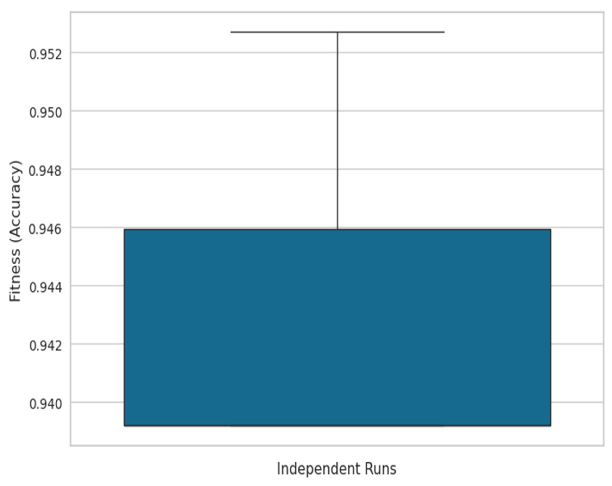
To provide a comprehensive evaluation, a box plot was generated (see Figure 3), where the x-axis represents independent ACO runs and the y-axis depicts the fitness function (accuracy), illustrating the stability and variance of the algorithm’s performance across multiple executions. Additionally, a convergence graph (see Figure 4) was plotted, with the x-axis representing iterations and the y-axis showing the best accuracy obtained over successive iterations, demonstrating the steady improvement in solution quality as the ACO progresses.

To validate the effectiveness of the ACO, a comparative analysis was conducted with particle swarm optimization (PSO). The results indicate that PSO selected 15 features, and an RF classifier using these features achieved an accuracy of 87.84%. In contrast, ACO selected the same number of features; however, RF using ACO-selected features achieved a significantly higher accuracy of 95.95%, highlighting the superiority of ACO in feature selection for this dataset. Additionally, a statistical significance test (T-test) was conducted to compare the accuracy distributions of ACO and PSO. The computed p-value was 0, confirming that the observed improvement in accuracy using ACO is statistically significant (p < 0.05) and not due to random chance.

The selection of ACO’s initialization parameters (number of ants, iterations, pheromone decay) was primarily based on insights from theoretical literature studies and previous studies in feature selection. These parameter settings were found to yield optimal performance in our problem context. Furthermore, one of the key challenges of ACO is its computational complexity, particularly in convergence time, which is O(m × n × I), where m is the number of ants, n is the number of features, and I is the number of iterations. Additionally, ACO is known to be sensitive to parameters such as pheromone decay, which can influence the balance between exploration and exploitation. These aspects should be carefully fine-tuned in practical applications to achieve an optimal trade-off between accuracy and computational efficiency.

Table 5. Experimental results of ML classifiers using a selected subset of ACO features.

Classifiers	Accuracy	AUC	Recall	Precision	F1-Score	Kappa	MCC
DT	89.50	89.47	92.11	87.93	89.85	78.98	79.32
RF	95.73	99.17	96.72	94.93	95.77	91.46	91.56
ET	97.70	99.55	98.37	97.15	97.73	95.41	95.47
Adaboost	91.47	97.24	92.49	90.99	91.57	82.95	83.27
XGB	95.08	99.03	96.41	94.18	95.14	90.17	90.45
LR	89.50	94.32	92.48	87.50	89.81	78.99	79.36
KNN	89.66	95.67	98.70	83.86	90.59	79.34	80.81

shows the experimental results employing feature subsets selected with the ACO method. Multiple ML classifiers were applied to the top 10 features that significantly impacted KD outcome prediction. The ET classifier outperformed the other models, with an accuracy of 97.70%, precision of 97.15%, recall of 98.37%, F1-score of 97.73%, and an AUC-ROC of 99.55% (marked as bold in Table 5). The accuracy of the other models varied, with DT achieving 89.50%, RF 95.73%, Adaboost 91.47%, XGB 95.08%, LR 89.50%, and KNN 89.66%. ET outperformed the other models, showing an improvement of 6.19% over processed complete feature sets (using an RF classifier with 91.51% accuracy). RF and XGB also demonstrated competitive and balanced performances, highlighting the effectiveness of the selected features in improving KD prediction accuracy.

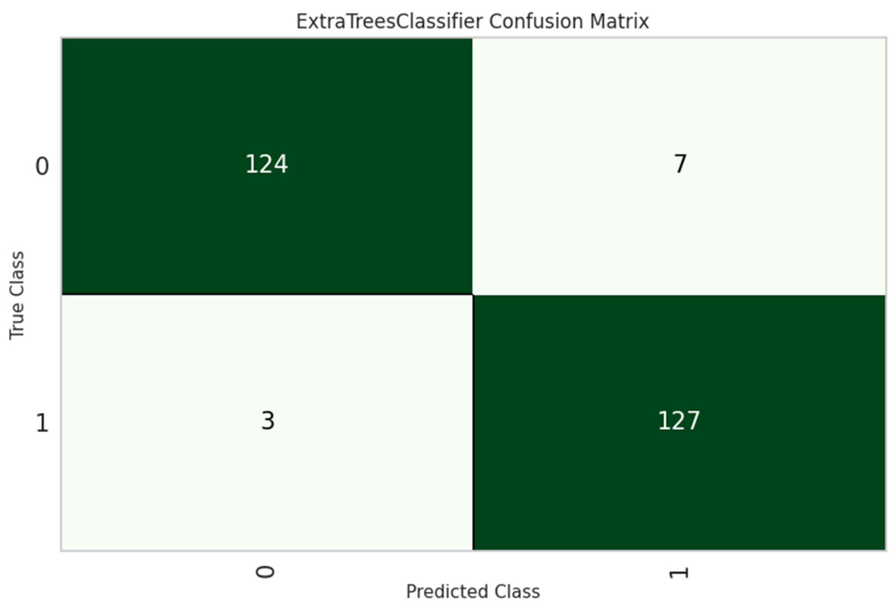
The ET classifier was the most effective model, with an accuracy of 97.70%, as shown in Table 5. Its architecture uses sequential tree development, in which every subsequent tree boosts efficiency by correcting the errors of its predecessors. ET achieved the highest accuracy by using the optimal combinations of hyperparameters as shown in

Table 6. ET classifier parameters with their optimal values.

Parameters	Value	Parameters	Value
bootstrap	False	min_samples_leaf	1
min_samples_split	2	random_state	123
max_features	sqrt	n_estimators	100
criterion	Gini	n_jobs	−1

. Furthermore, its performance was thoroughly investigated and analyzed using the confusion matrix and the ROC curve, which provided more insight into its classification competencies, as seen in Figure 5 and Figure 6.

The RF and XGB models performed competitively, with AUC values of 99.17% and 99.03%, respectively. The ROC curves for these models are also shown in Figure 7 for comparison. Although their accuracies (RF: 95.95%;t XGB: 95.08%) were lower than that for ET, the high AUC scores show that they have a significant discriminatory potential. Based on the ROC curve comparisons, it is evident that ET, RF, and XGB all show outstanding classification skills, with ET attaining the highest overall performance. The ROC curves help choose the best classifier for a situation by evaluating model efficacy more thoroughly.

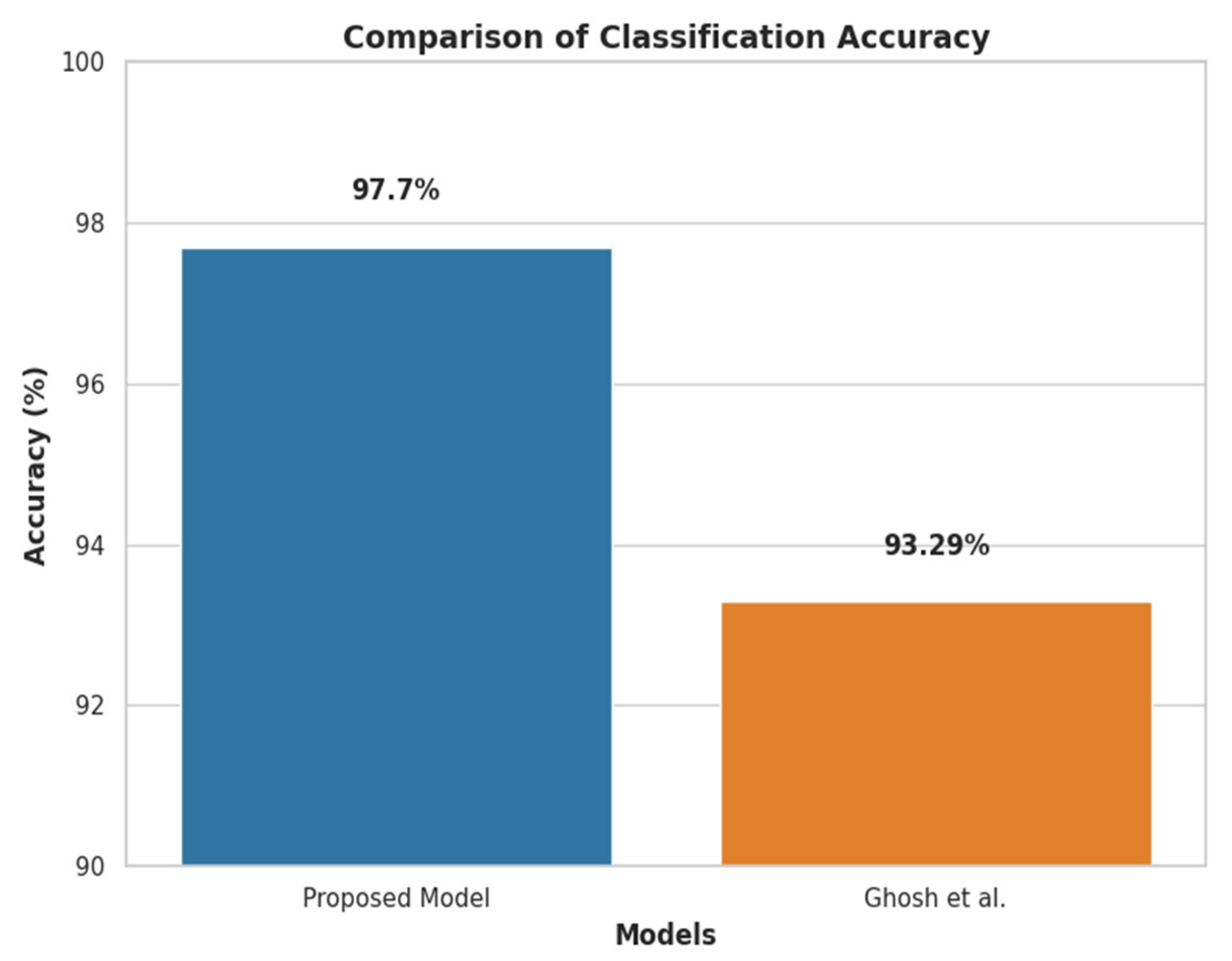
5.3. Performance Comparison with State-of-the-Art Techniques

Figure 8 compares the proposed approach with the previous most advanced KD prediction strategy [26], which obtained the previous best accuracy of 93.29% in identifying KD patients. With the same clinical KD dataset, which included 1,023,426 samples with a 1.20% positive ratio, the proposed approach significantly outperformed the previous benchmark by 4.41% and achieved a 97.70% accuracy.

5.4. Explainable SHAP Analysis

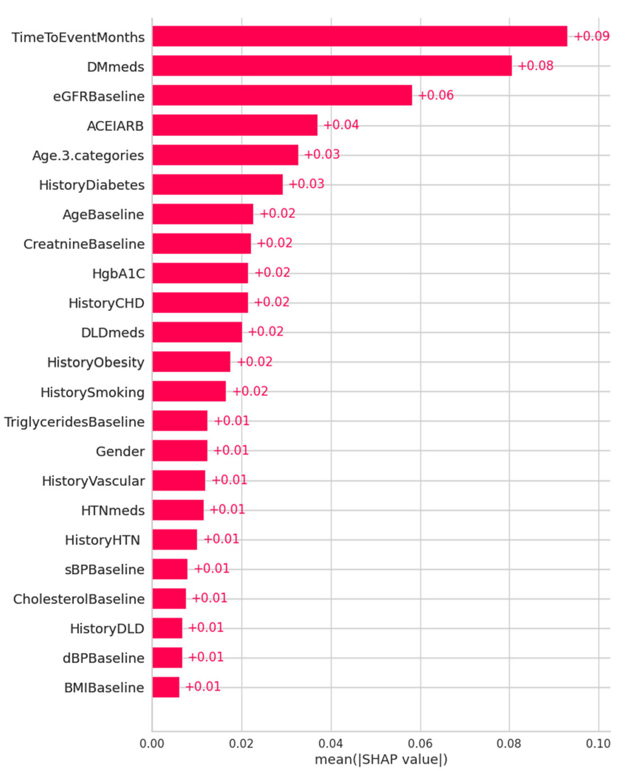
Evaluating the local and global interpretability of predictive models is imperative, especially in classification frameworks, where models related to prediction significantly impact performance. The ET algorithm is appropriate for current medical clinical data analysis because of its notable model performance and execution speed. SHAP offers a potent method for feature interpretability, and its waterfall charts, summary, and SHAP values are practical tools for explaining how each feature contributes to the model’s output.

Figure 9 shows the feature importance ranking in descending order using mean SHAP values for the ET model, with mean SHAP values on the x-axis and feature rankings on the y-axis. It indicates that TimeToEventMonths, DMmeds, eGFRBaseline, ACEIARB, and Age are the most important predictors. Features with higher SHAP values are more important in predicting outcomes, as the plot shows.

Figure 10 shows the SHAP summary plots for both ET and RF models. The summary plots thoroughly explain how individual distinctive features contribute to the significance of the target variable in prediction. Features are sorted by importance on the y-axis, which shows the strength and direction of the feature correlation with the desired result, while the x-axis shows SHAP values. While negative numbers indicate an adverse effect, positive SHAP values positively impact the prediction. Every line in the plot represents a unique feature: higher feature values are shown in red, while lower values are indicated in blue. This color combination offers insights into the connection between feature values and prediction.

A comparison of the top five primary features of both models indicates substantial variations between them. The ET model prioritizes TimeToEventMonths, DMmeds, eGFRBaseline, ACEIARB, and Age, while the RF model highlights TimeToEventMonths, DMmeds, eGFRBaseline, HgbA1C, and dBPBaseline as the most important predictors. This comparison shows similarities in major clinical parameters, including TimeToEventMonths, DMmeds, and eGFRBaseline, and variances in secondary relevant variables. Given that ACEIARB is included in ET and HgbA1C is included in RF, ET may emphasize medication-related aspects more, whereas RF gives metabolic indications more weight. This comparative SHAP analysis provides insights into the relevance of features across multiple classifiers and further verifies the interpretability of the ET model. It also shows how RF is based on predictive reasoning.

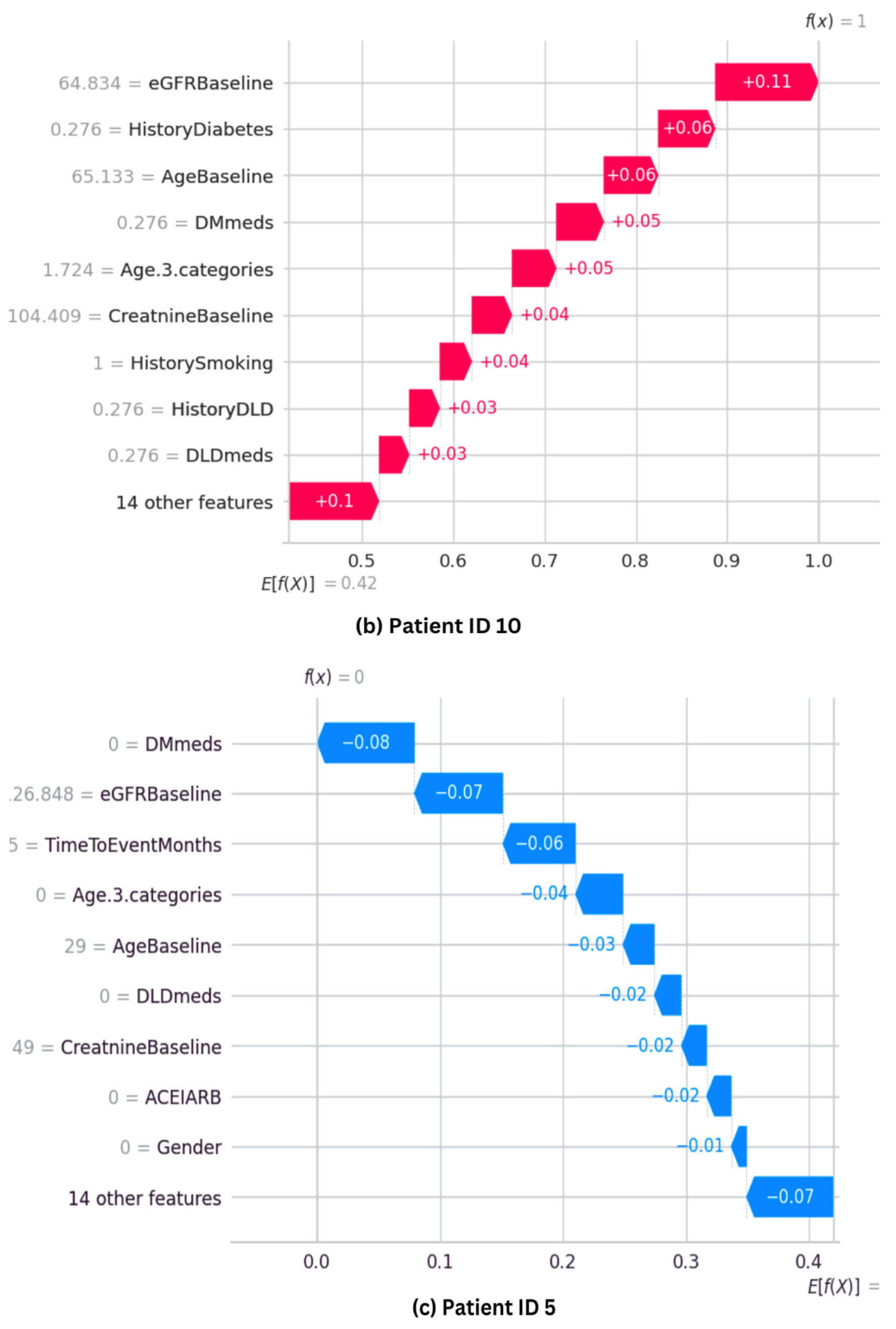
The SHAP waterfall plot for the ET model is shown in Figure 11, where each feature’s magnitude indicates its impact on the final prediction. The feature’s effect on the model’s output directly correlates with the bar size. The ET model’s predictive probability was analyzed for three randomly selected patients, and the features’ contribution to the prediction were plotted as shown in Figure 11. Positive impacts (shown in red) raise the projected outcome from the base value in a waterfall plot, while negative effects (shown in blue) lower it. Every step in the waterfall plot represents a different feature’s contribution; the length of the step indicates the feature’s size of impact, and the direction (up or down) indicates whether it raises or lowers the predictions.

Figure 11a shows that Patient ID 0 has a predictive probability value [f(x)] of 1. The top positive contributors, such as TimeToEventMonths, DMmeds, eGFRBaseline, HistoryCHD, and ACEIARB, improve prediction. However, HistoryObestiy, one of the ten plot elements, has a negative impact. Figure 11b shows Patient ID 10’s predictive probability is 1, comparable with that of Patient ID 0. Features such as Age, HistoryDiabetes, eGFRBaseline, and DMmeds significantly influence the final prediction. Figure 11c shows that Patient ID 5 has a predicted probability value [f(x)] of zero. It shows that almost every feature hurts the prediction. However, eDGRBaseline, TimeToEventMonths, and DMmeds make negative model predictions.

According to the SHAP analysis, various features were consistently found as having considerable predictive potential across various patient situations. TimeToEventMonths, DMmeds, eGFRBaseline, ACEIARB, and Age have been identified as significant predictors of KD development, supporting relevant clinical knowledge. For example, TimeToEventMonths shows the time from diagnosis, which is essential in determining how far along a disease is. Similarly, DMmeds (diabetic medicines) indicate the significance of managing concurrent medical conditions such as diabetes, a well-known risk factor for kidney disease. eGFRBaseline, an essential indicator of kidney function, is directly and rationally correlated with the severity of the disease. The ACEIARB feature pertains to the usage of certain drugs that are often recommended to treat kidney-related complications, especially in patients with KD. Lastly, Age is a broad but essential risk factor, with a higher risk of KD being associated with older age. These factors play a vital role in clinical decision-making, meaning that the model’s significance is practical and can be put into practice. Using these insights, clinicians may prioritize monitoring and modifying treatment strategies, particularly for patients with large values in these aspects. For example, they might increase the dose of ACEIARB medicines or strengthen monitoring for patients whose illness stage is fast progressing. It is crucial to match these model predictions with clinical practices to improve patient outcomes. It will guarantee that the findings can be adequately transformed into actionable clinical decisions.

Challenges in SHAP Implementation

Although SHAP offers practical interpretability for feature significance, its use has several challenges. Computational efficiency is essential, mainly when dealing with vast amounts of data or complex models. KernelSHAP, in particular, demands significant computing time, which might slow down analysis. However, Tree-SHAP improves this for tree-based models. Feature correlations also impact SHAP values, making it challenging to distinguish between independent feature contributions. Feature grouping and dependent plots were utilized to overcome this by enhancing interpretability. Additionally, domain expertise is necessary to convert SHAP results into clinically actionable insights, as certain features with high SHAP values may not always correspond directly to anticipated medical knowledge. By overcoming these challenges, SHAP will continue to be a strong and trustworthy tool for interpreting models.

5.5. Explainable LIME Analysis

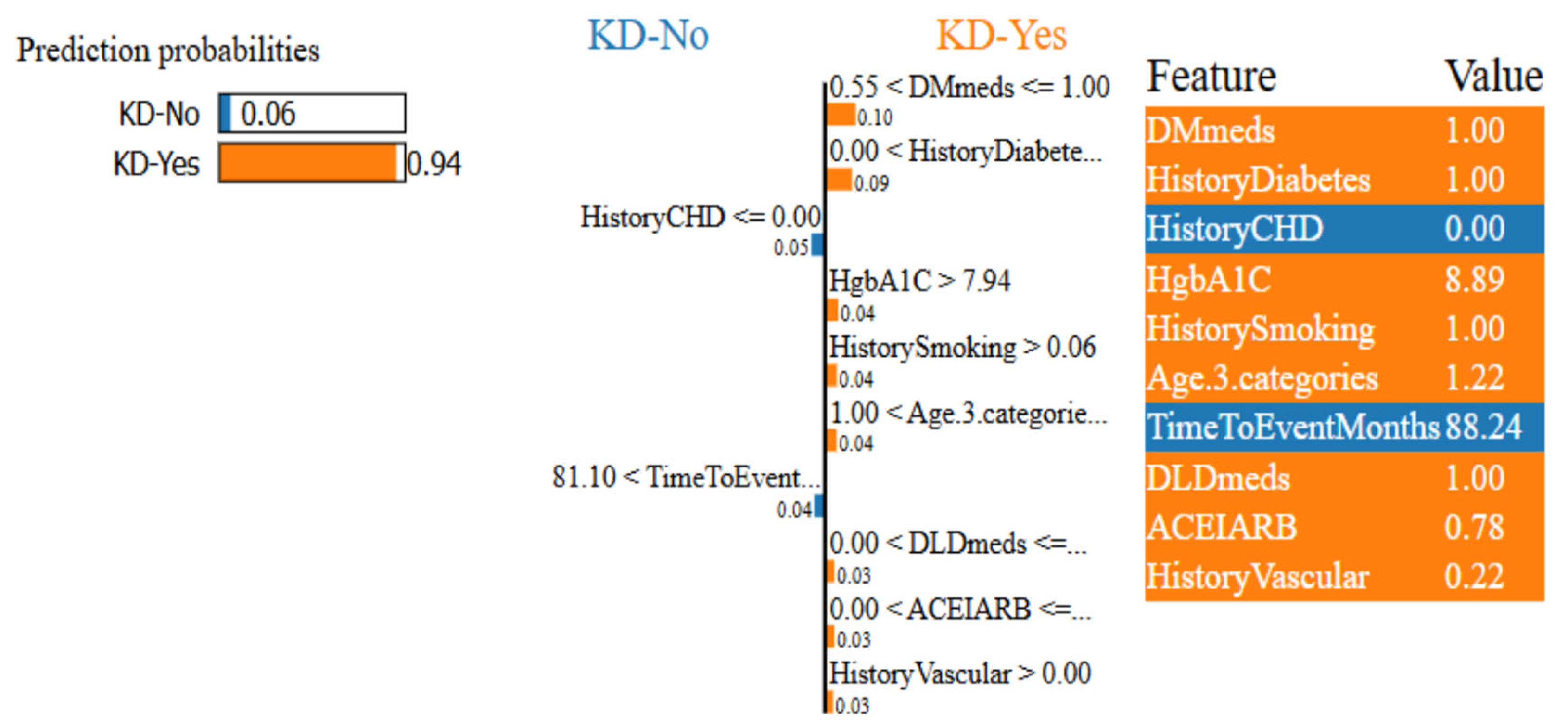
LIME approaches were also used to examine and interpret predictions from the ML models, both locally and globally. Figure 12 and Figure 13 provide random instances for local interpretation, emphasizing features that affected the differentiation of patients into KD-Yes (1, shown in orange) or KD-No (0, shown in blue). The visualizations provide the precise values of these characteristics and information about how they contributed to the prediction.

Each figure has three parts: left, center, and right. The anticipated results for each patient in both classes (0 or 1) are shown in the left section. The center part lists the top 10 significant characteristics that drive the classifications, in descending order of importance. Longer bars signify a larger influence on the predicted features, and each bar’s length represents the importance of the relevant feature. The important characteristics of these prominent features at their maximum contribution to the prediction are highlighted in the rightmost area.

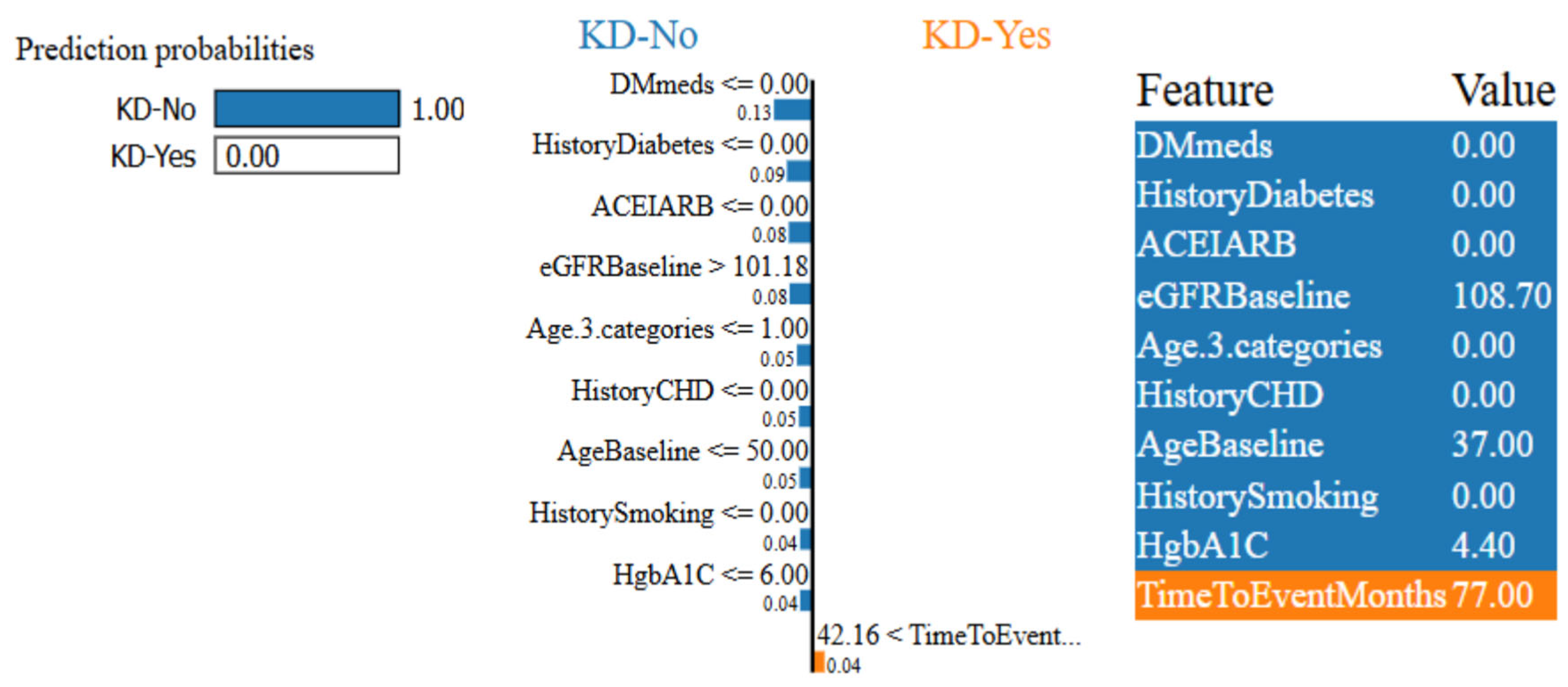
Figure 12 and Figure 13 show that the ET model has a 94% confidence interval in predicting KD-Yes for Patient ID 55 (Figure 12). Features like DMmeds, HistoryDiabetes, and HgbA1C significantly impact the prediction toward KD-Yes, while TimeToEventMonths and HistoryCHD endorse KD-No for this patient. Patient ID 63, on the other hand, is 100% confidently identified as KD-No in Figure 13. TimeToEventMonths is the sole factor that marginally supports KD-Yes, but DMmeds, HistoryDiabetes, ACEIARB, and eGFRBaseline are key features that affect this prediction. The interpretability of the model’s predictions is improved by these visual charts, which provide insightful information about the contributions of input features.

The global feature importance for KD prediction using the ET classifier, as examined using LIME, is shown in Figure 14. The most important factors that greatly assist in predicting KD are DMmeds, HistoryDiabetes, DLDmeds, and HistoryCHD. On the other hand, characteristics like ACEIARB, TimeToEventMonths, and HistoryHTN show the most negative significance, lowering the risk of KD development and reflecting clinical markers of improved kidney health. Features such as HistoryVascular and HistorySmoking have minimal impact, suggesting that they are irrelevant to the dataset. This study emphasizes the interpretability of the model and identifies important factors that affect the results of KD classification.

The LIME analysis offers valuable insights into the factors influencing KD prediction. In line with clinical understanding, the most influential features identified in local and global interpretations include DMmeds, HistoryDiabetes, HgbA1C, eGFRBaseline, HistoryCHD, and ACEIARB. For example, DMmeds and HistoryDiabetes strongly contribute to predicting the presence of KD, aligning with the established clinical notion that diabetes is a significant risk factor for kidney disease. HgbA1C is crucial for monitoring long-term blood glucose control, directly impacting kidney health in diabetic patients. Similarly, eGFRBaseline is a highly relevant feature, reflecting the clinical practice of using eGFR to assess KD progression. HistoryCHD also makes a significant contribution, as cardiovascular health is closely linked with kidney function in KD patients.

Interestingly, features such as ACEIARB, a class of drugs commonly used to protect kidney function, and TimeToEventMonths, reflecting disease progression, were associated with lower predictions for CKD risk, consistent with their use in slowing kidney disease progression. The LIME results highlight the importance of these key features in helping clinicians interpret and refine diagnostic and treatment strategies. For instance, if a patient exhibits high values for DMmeds, HistoryDiabetes, and HgbA1C, clinicians may decide to intensify their diabetes management. On the other hand, for patients with low risks in ACEIARB and eGFRBaseline, treatment protocols may focus on preventive measures and lifestyle changes. These insights enable clinicians to make more informed decisions, tailoring treatment to the patient’s risk profile and potentially improving clinical outcomes.

5.6. Ethical Implications

Integrating AI in medical decision-making presents ethical challenges, particularly regarding the consequences of incorrect predictions. False positives may lead to unnecessary medical interventions, causing patient anxiety and resource misallocation, while false negatives could result in delayed treatment and worsened health outcomes. We emphasize model interpretability through SHAP analysis to mitigate these risks, allowing clinicians to understand feature contributions and validate predictions. Additionally, rigorous model validation across diverse patient groups, periodic reassessment of performance, and integration of expert oversight into AI-assisted decisions can enhance reliability. Ensuring transparency in AI-driven predictions fosters trust among healthcare professionals and patients, ultimately supporting safe and ethical deployment in clinical practice.

6. Conclusions

This paper presents an interpretable ML framework for predicting chronic kidney disease, incorporating metaheuristic ACO-based feature selection to enhance model performance. The ACO-based feature selection approach effectively improves KD prediction by identifying the most relevant clinical features, increasing diagnosis accuracy while reducing unnecessary tests. This is particularly beneficial in real-world medical settings, where minimizing diagnostic time and costs is critical. Multiple ML classifiers, including LR, RF, NB, DT, ET, and XGB, were evaluated, with ET achieving the highest accuracy of 97.7% and an AUC of 99.55% when using ACO-selected features.

Beyond predicted accuracy, we improved the interpretability of the model by using SHAP and LIME approaches, providing both local and global explanations of decision-making processes. These enhance the model’s reliability and clinical applicability by ensuring interpretability for medical practitioners. This approach has significant potential for integration with AI-powered clinical decision-support systems, enabling healthcare professionals to make more informed and accurate diagnoses. The approach is a vital addition to AI-driven healthcare, and its versatility implies that it might also be used to anticipate other medical conditions.

Despite its benefits, the suggested ACO-based feature selection approach has a few limitations. First, ACO exhibits more computational complexity than conventional feature selection methods, potentially restricting its scalability for complex datasets. Second, the performance of ACO is highly dependent on hyperparameter optimization, requiring the diligent selection of parameters, such as the number of ants and the rate of pheromone decay. Although we only compared ACO and PSO, comparing them to other new metaheuristic optimizers would be beneficial. Finally, the model should be evaluated on various datasets to verify its generalizability and to prevent overfitting. Future studies should investigate the use of deep learning approaches to improve the model’s adaptability and resilience in dealing with complex CKD patterns. The model’s generalizability will be further confirmed by expanding the dataset to include a range of patient demographics. Moreover, real-time implementation in clinical environments and association with electronic health records (EHRs) might connect AI-driven diagnoses with practical medical applications. By solving these issues, future developments in AI-driven CKD diagnosis might greatly enhance early detection and patient outcomes, resulting in improved nephrology treatment.