
The Condition Evaluation of Bridges Based on Fuzzy BWM and Fuzzy Comprehensive Evaluation

 ,
,
Abstract
1. Introduction
2. Fuzzy Best and Worst Method-Fuzzy Comprehensive Evaluation Model
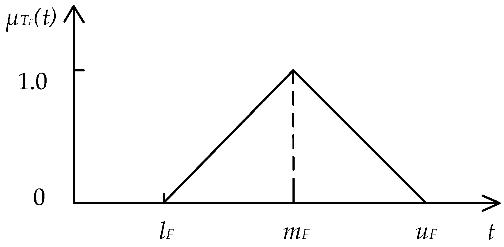
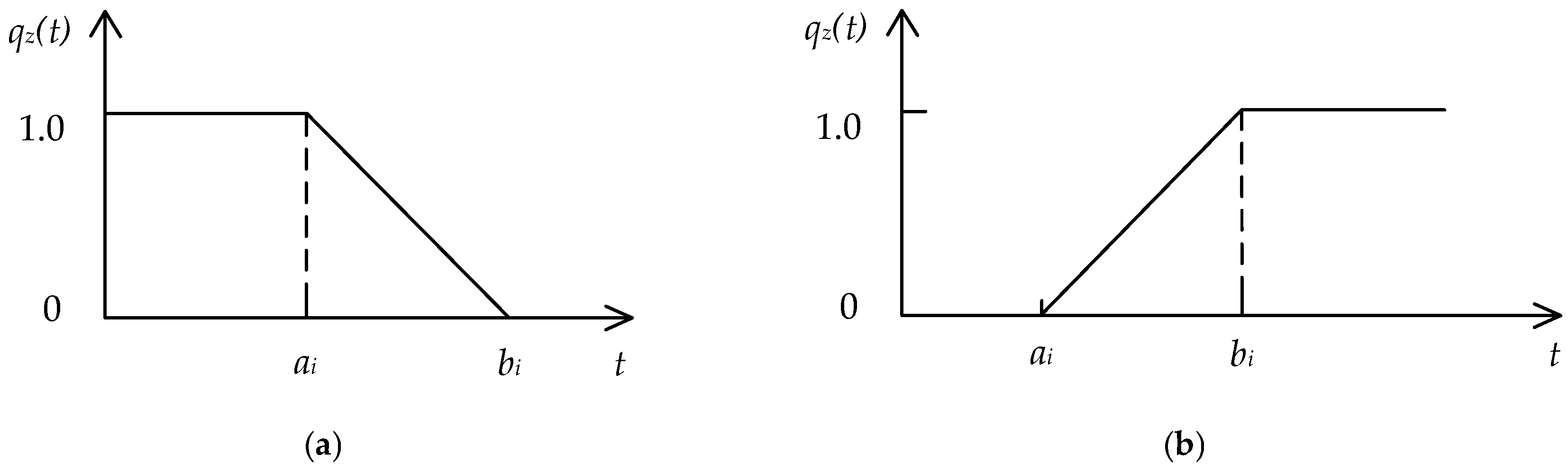
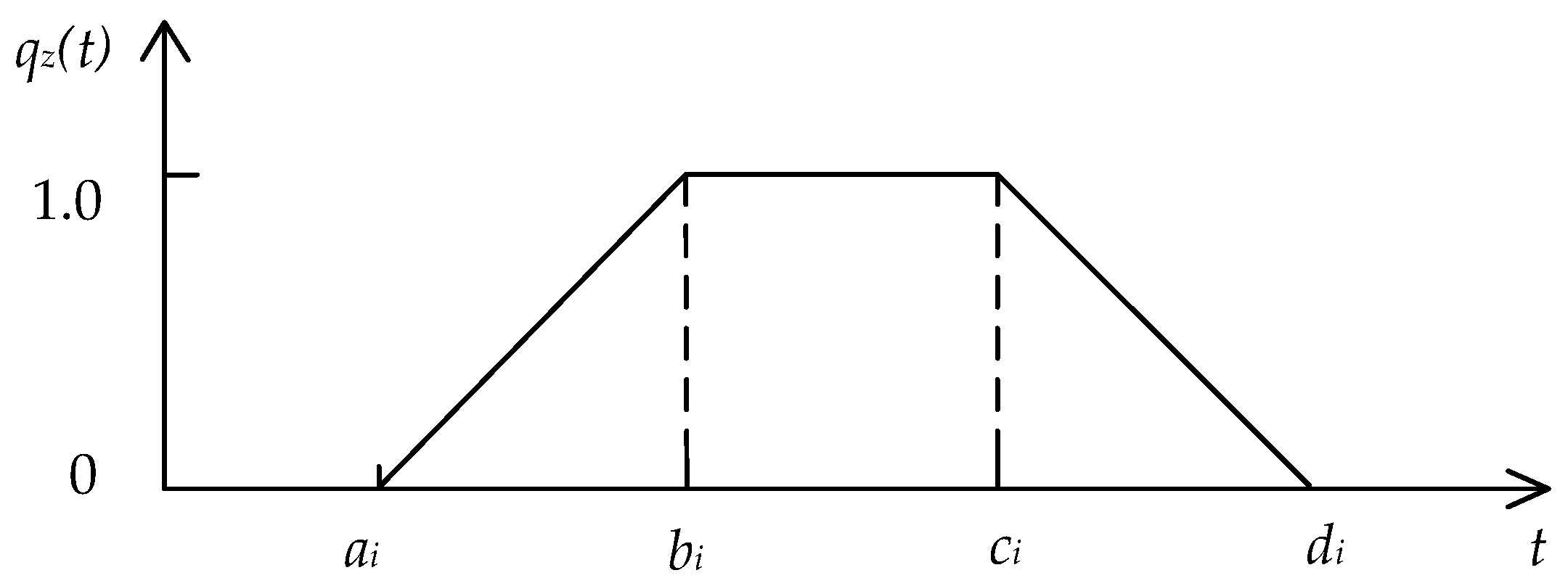
2.1. Fuzzy Set and Membership Function
2.2. Fuzzy Best and Worst Method

| Five Levels of Importance | Identically Important (II) | Slightly Important (SI) | Relatively Important (RI) | Highly Important (HI) | Extremely Important (EI) |
|---|---|---|---|---|---|
| CI | 3.00 | 3.8 | 5.29 | 6.69 | 8.04 |
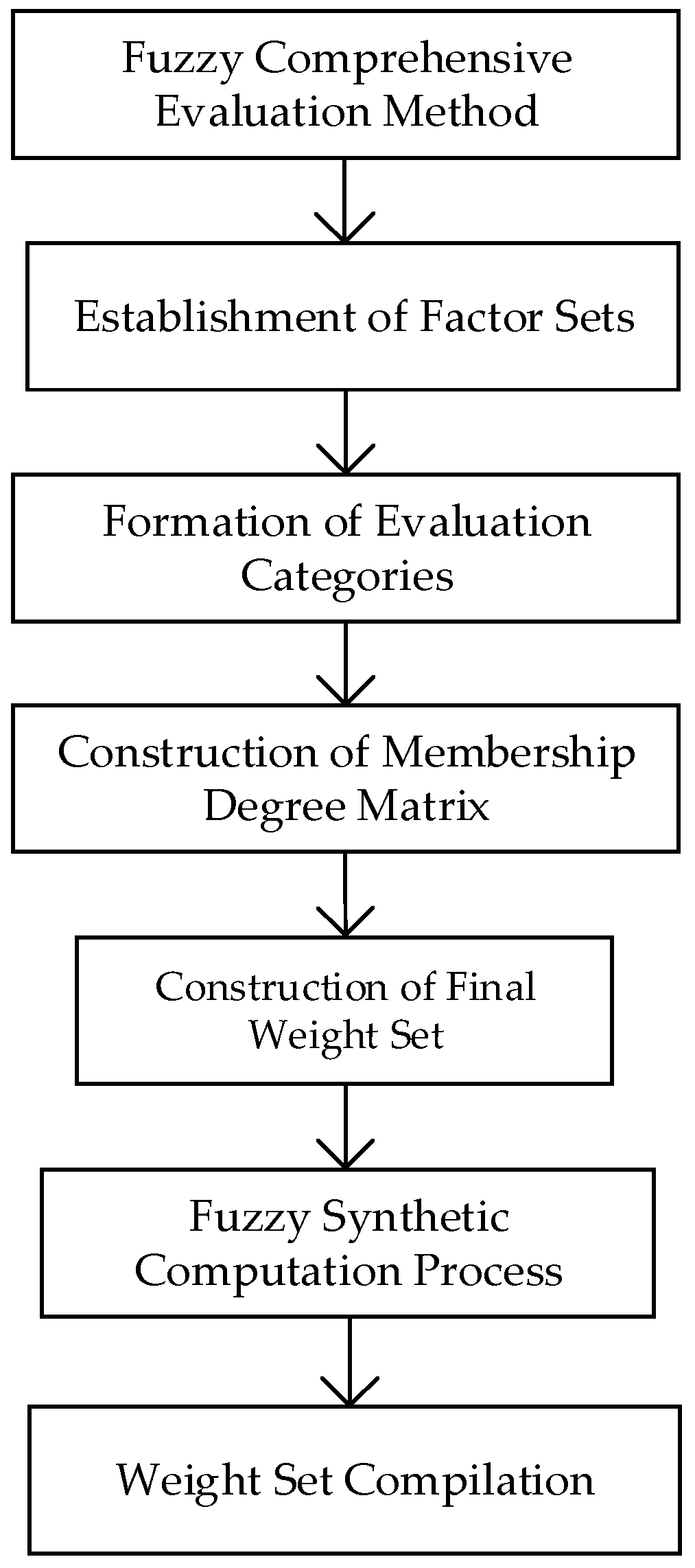
2.3. Fuzzy Comprehensive Evaluation
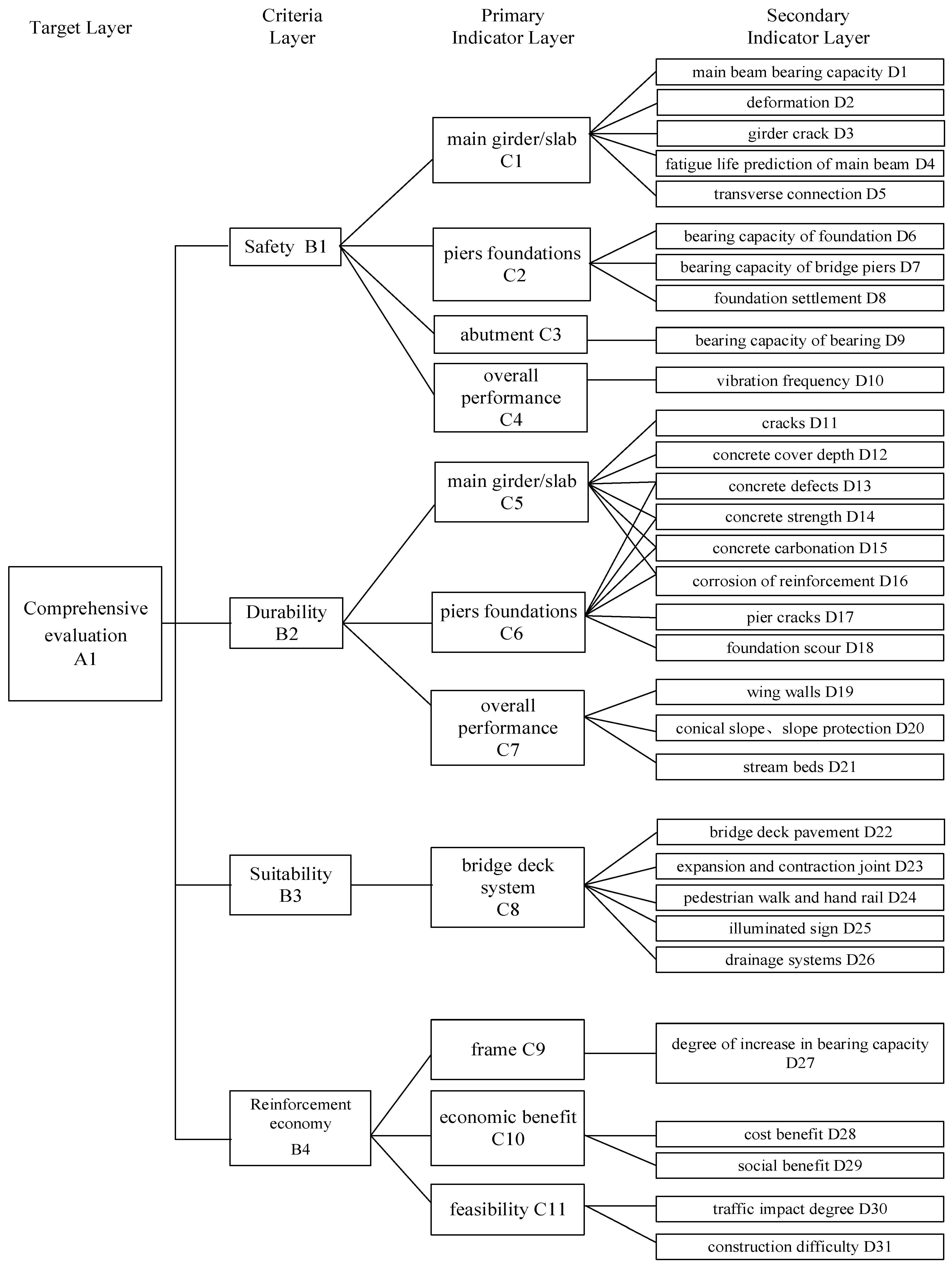
3. Condition Evaluation Indicator System for Bridges
3.1. Principles for Selecting Indicators
3.2. Establishing the Indicator System
4. Case Study
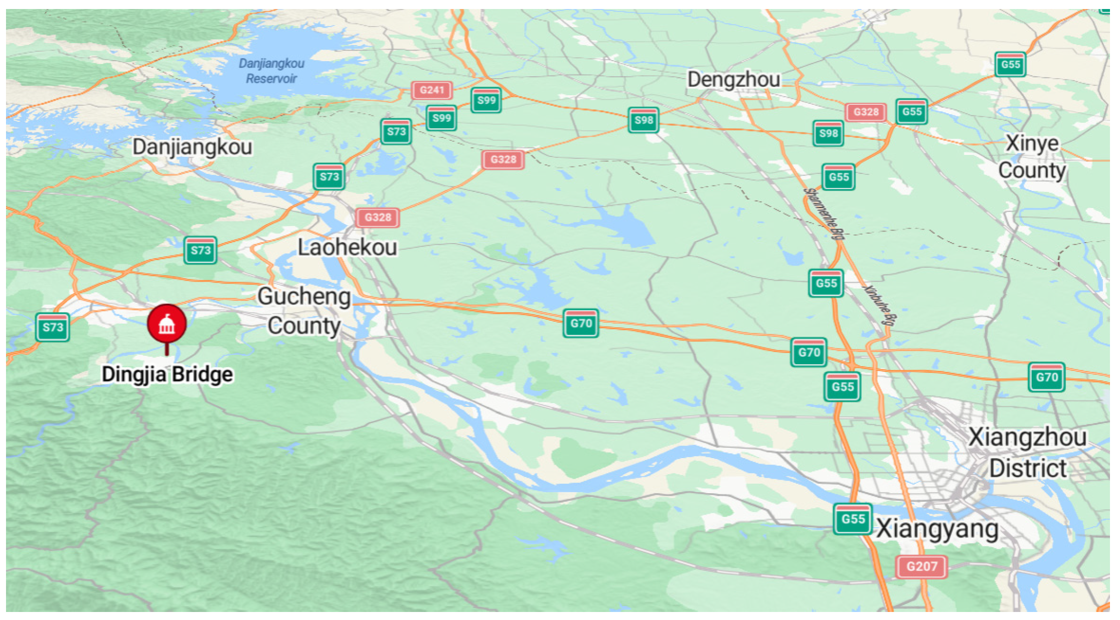
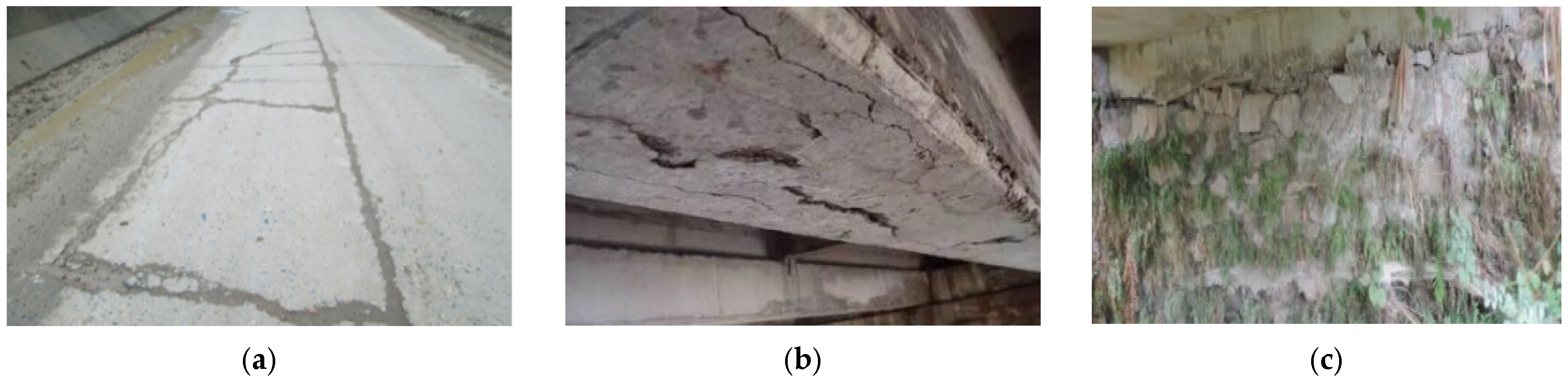
4.1. Case Study 1
4.1.1. Weight Calculation for Dingjia Bridge
4.1.2. Condition Rating of Dingjia Bridge
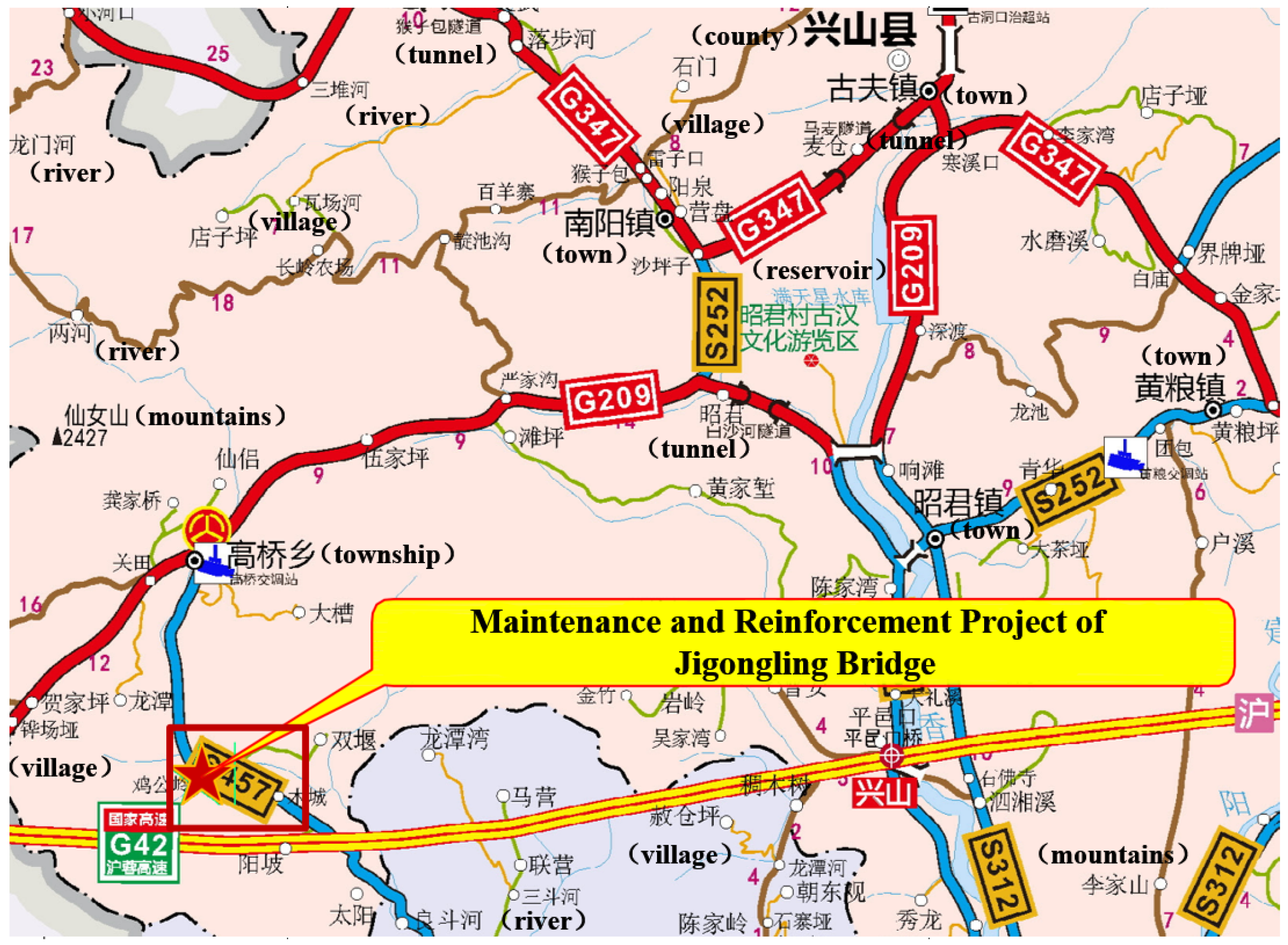
4.2. Case Study 2
4.2.1. Weight Calculation for Jigongling Bridge
4.2.2. Condition Rating of Jigongling Bridge
5. Conclusions
- Model Introduction and Comparative Analysis: This study presents a novel integrated evaluation model that synergistically combines the FBWM and FCE methods to address uncertainties and enhance operational efficiency in bridge condition evaluation. The proposed FBWM-FCE model firstly establishes a four-layer indicator system, ensuring the system’s alignment with the structural characteristics of bridges and regulatory requirements. Subsequently, by introducing TFNs to quantify linguistic ambiguities in the bridge’s expert judgments, the model reduces cognitive bias compared to the conventional BWM, achieving a CR of 19.7%, which is 22% lower than BWM and AHP, respectively. This innovation streamlines decision-making, requiring 20% fewer pairwise comparisons than AHP while maintaining robust methodological consistency.
- Case Validation: The practical efficacy of the FBWM-FCE model was validated through case studies of Ding Jia Bridge and Jigongling Bridge in Hubei Province, China. Evaluations of both bridges according to the FBWM-FCE demonstrated full alignment with on-site inspections documented in the 2020 Bridge Inspection and Evaluation Report issued by the Highway Administration of Hubei Provincial Department of Transportation. The model’s reliability was further corroborated by its consistent outcomes with conventional standardized methods, while overcoming their limitations in procedural complexity and operational inefficiency.
- Practical Application Significance, Limitations, and Future: A distinctive contribution of this research lies in its pioneering application of FBWM to bridge condition evaluation. The hybrid methodology reduces reliance on rigid numerical scales, decreasing subjective bias in weight determination processes, particularly in handling ambiguous expert judgments and multi-criteria interactions. Furthermore, the developed indicator system demonstrated exceptional adaptability to diverse bridge typologies, particularly small-to-medium span structures, as evidenced by its successful implementation in the Hubei Provincial Highway Bridge maintenance project. However, the current research on the real-time monitoring of bridge condition and the evaluation of long-span bridges is still not sufficient, and improvements can be made to the following aspects in the future: extending the model to long-span bridges, incorporating real-time sensor data for dynamic condition monitoring, and developing AI-driven automation for large-scale network-level evaluations. These advancements promote the proposed methodology as a transformative solution for modern infrastructure management while balancing theoretical innovation with engineering pragmatism.
Author Contributions
Funding
Institutional Review Board Statement
Informed Consent Statement
Data Availability Statement
Acknowledgments
Conflicts of Interest
References
- Feng, Q.; Kong, Q.; Tan, J.; Song, G. Grouting compactness monitoring of concrete-filled steel tube arch bridge model using piezoceramic-based transducers. Smart Struct. Syst. 2017, 20, 175–180. [Google Scholar] [CrossRef]
- Feng, Q.; Xiao, H.; Kong, Q.; Liang, Y.; Song, G. Damage detection of concrete piles subject to typical damages using piezoceramic based passive sensing approach. J. Vibroeng. 2016, 18, 801–812. [Google Scholar] [CrossRef]
- Tan, J.; Jiang, J.; Liu, M.; Feng, Q.; Zhang, P.; Ho, S.C.M. Implementation of shape memory alloy sponge as energy dissipating material on pounding tuned mass damper: An experimental investigation. Appl. Sci. 2019, 9, 1079. [Google Scholar] [CrossRef]
- Weinstein, J.C.; Sanayei, M.; Brenner, B.R. Bridge damage identification using artificial neural networks. J. Bridge Eng. 2018, 23, 04018084. [Google Scholar] [CrossRef]
- Fard, F.; Sadeghi Naieni, F. Development and utilization of bridge data of the United States for predicting deck condition rating using random forest, XGBoost, and artificial neural network. Remote Sens. 2024, 16, 367. [Google Scholar] [CrossRef]
- Feng, Q.; Cui, J.; Wang, Q.; Fan, S.; Kong, Q. A feasibility study on real-time evaluation of concrete surface crack repairing using embedded piezoceramic transducers. Measurement 2018, 122, 591–596. [Google Scholar] [CrossRef]
- Comisu, C.C.; Taranu, N.; Boaca, G.; Scutaru, M.C. Structural health monitoring system of bridges. Procedia Eng. 2017, 199, 2054–2059. [Google Scholar] [CrossRef]
- Guo, J.; Zhang, Y.; Yuan, G.; Li, Y.; Wang, L.; Dong, Z. A Large Bridge Traffic Operation Status Impact Assessment Model Based on AHP–Delphi–SVD Method. Appl. Sci. 2024, 14, 9327. [Google Scholar] [CrossRef]
- Ors, D.M.; Ebid, A.M.; Mahdi, I.M.; Mahdi, H.A. Decision support system to select the optimum construction techniques for bridge piers. Ain Shams Eng. J. 2023, 14, 102152. [Google Scholar] [CrossRef]
- Lu, Z.; Wei, C.; Liu, M.; Deng, X. Risk assessment method for cable system construction of long-span suspension bridge based on cloud model. Adv. Civ. Eng. 2019, 2019, 5720637. [Google Scholar] [CrossRef]
- Darban, S.; Ghasemzadeh Tehrani, H.; Karballaeezadeh, N.; Mosavi, A. Application of analytical hierarchy process for structural health monitoring and prioritizing concrete bridges in iran. Appl. Sci. 2021, 11, 8060. [Google Scholar] [CrossRef]
- Hussain, A.; Chun, J.; Khan, M. A novel multicriteria decision making (MCDM) approach for precise decision making under a fuzzy environment. Soft Comput. 2021, 25, 5645–5661. [Google Scholar] [CrossRef]
- Rezaei, J. Best-worst multi-criteria decision-making method. Omega 2015, 53, 49–57. [Google Scholar] [CrossRef]
- Khan, M.S.A.; Etonyeaku, L.C.; Kabir, G.; Billah, M.; Dutta, S. Bridge infrastructure resilience assessment against seismic hazard using Bayesian best worst method. Can. J. Civ. Eng. 2022, 49, 1669–1685. [Google Scholar] [CrossRef]
- Giordano, P.F.; Limongelli, M.P. The value of structural health monitoring in seismic emergency management of bridges. Struct. Infrastruct. Eng. 2022, 18, 537–553. [Google Scholar] [CrossRef]
- Xu, Y.; Zhu, X.; Wen, X.; Herrera-Viedma, E. Fuzzy best-worst method and its application in initial water rights allocation. Appl. Soft Comput. 2021, 101, 107007. [Google Scholar] [CrossRef]
- Moslem, S.; Gul, M.; Farooq, D.; Celik, E.; Ghorbanzadeh, O.; Blaschke, T. An integrated approach of best-worst method (BWM) and triangular fuzzy sets for evaluating driver behavior factors related to road safety. Mathematics 2020, 8, 414. [Google Scholar] [CrossRef]
- Bahrami, S.; Rastegar, M.; Dehghanian, P. An FBWM-TOPSIS approach to identify critical feeders for reliability centered maintenance in power distribution systems. IEEE Syst. J. 2020, 15, 3893–3901. [Google Scholar] [CrossRef]
- Malakoutikhah, M.; Alimohammadlou, M.; Jahangiri, M.; Rabiei, H.; Faghihi, S.A.; Kamalinia, M. Modeling the factors affecting unsafe behaviors using the fuzzy best–worst method and fuzzy cognitive map. Appl. Soft Comput. 2022, 114, 108119. [Google Scholar] [CrossRef]
- Irannezhad, M.; Shokouhyar, S.; Ahmadi, S.; Papageorgiou, E.I. An integrated FCM-FBWM approach to assess and manage the readiness for blockchain incorporation in the supply chain. Appl. Soft Comput. 2021, 112, 107832. [Google Scholar] [CrossRef]
- Jahangiri, S.; Shokouhyar, S. An integrated FBWM-FCM-DEMATEL model to assess and manage sustainability in the supply chain: A three-stage model based on the consumers’ point of view. Appl. Soft Comput. 2024, 157, 111281. [Google Scholar] [CrossRef]
- Gul, M.; Yucesan, M.; Celik, E. A manufacturing failure mode and effect analysis based on fuzzy and probabilistic risk analysis. Appl. Soft Comput. 2020, 96, 106689. [Google Scholar] [CrossRef]
- JTG 5120-2004; Specification for Maintenance of Highway Bridges and Culverts. China Standard: Beijing, China, 2004.
- Zadeh, L.A. Fuzzy sets. Inf. Control 1965, 8, 338–353. [Google Scholar] [CrossRef]
- Chou, C.C. The canonical representation of multiplication operation on triangular fuzzy numbers. Comput. Math. Appl. 2003, 45, 1601–1610. [Google Scholar] [CrossRef]
- Zhao, H.; Guo, S. Selecting green supplier of thermal power equipment by using a hybrid MCDM method for sustainability. Sustainability 2014, 6, 217–235. [Google Scholar] [CrossRef]
- Zhang, W.; Huang, Z.; Zhang, J.; Zhang, R.; Ma, S. Multifactor uncertainty analysis of construction risk for deep foundation pits. Appl. Sci. 2022, 12, 8122. [Google Scholar] [CrossRef]
- Gupta, H. Assessing organizations performance on the basis of GHRM practices using BWM and Fuzzy TOPSIS. J. Environ. Manag. 2018, 226, 201–216. [Google Scholar] [CrossRef]
- Guo, S.; Zhao, H. Fuzzy best-worst multi-criteria decision-making method and its applications. Knowl.-Based Syst. 2017, 121, 23–31. [Google Scholar] [CrossRef]
- Dong, J.; Wan, S.; Chen, S.M. Fuzzy best-worst method based on triangular fuzzy numbers for multi-criteria decision-making. Inf. Sci. 2021, 547, 1080–1104. [Google Scholar] [CrossRef]
- Ecer, F.; Pamucar, D. Sustainable supplier selection: A novel integrated fuzzy best worst method (F-BWM) and fuzzy CoCoSo with Bonferroni (CoCoSo’B) multi-criteria model. J. Clean. Prod. 2020, 266, 121981. [Google Scholar] [CrossRef]
- Kumar, A.; Anbanandam, R. Assessment of environmental and social sustainability performance of the freight transportation industry: An index-based approach. Transp. Policy 2022, 124, 43–60. [Google Scholar] [CrossRef]
- Wei, D.; Du, C.; Lin, Y.; Chang, B.; Wang, Y. Thermal environment assessment of deep mine based on analytic hierarchy process and fuzzy comprehensive evaluation. Case Stud. Therm. Eng. 2020, 19, 100618. [Google Scholar] [CrossRef]
- Xu, X.; Nie, C.; Jin, X.; Li, Z. A comprehensive yield evaluation indicator based on an improved fuzzy comprehensive evaluation method and hyperspectral data. Field Crops Res. 2021, 270, 108204. [Google Scholar] [CrossRef]
- Wu, D. Twelve considerations in choosing between Gaussian and trapezoidal membership functions in interval type-2 fuzzy logic controllers. In Proceedings of the 2012 IEEE International Conference on Fuzzy Systems, Brisbane, QLD, Australia, 10–15 June 2012; pp. 1–8. [Google Scholar] [CrossRef]
- Xue, B.; Lu, F.; Guo, J.; Wang, Z.; Zhang, Z.; Lu, Y. Research on energy efficiency evaluation model of substation building based on AHP and fuzzy comprehensive theory. Sustainability 2023, 15, 14493. [Google Scholar] [CrossRef]
- JTG/T H21-2011; Standard for Technical Condition Evaluation of Highway Bridges. China Standard: Beijing, China, 2011.
- Hubei Provincial Department of Transport Highway Administration Bureau. 2020 Bridge Inspection and Evaluation Report; Hubei Provincial Department of Transport Highway Administration Bureau: Wuhan, China, 2020. [Google Scholar]
- Li, Y.; Zhang, Z.; Chen, J.; Peng, H. Bridge comprehensive evaluation method based on BWM and fuzzy theory. J. Chongqing Jiaotong Univ. (Nat. Sci. Ed.) 2023, 42, 9–14+22. [Google Scholar]


| Five-Level Importance Scale | TFN |
|---|---|
| Identically Important (II) | |
| Slightly Important (SI) | |
| Relatively Important (RI) | |
| Highly Important (HI) | |
| Extremely Important (EI) |
| Indicator | B1 | B2 | B3 | B4 |
|---|---|---|---|---|
| Best Indicator B1 | II | SI | HI | EI |
| Worst Indicator B4 | EI | HI | RI | II |
| Criteria Layer | Final Weights | Primary Indicator Layer | Final Weights | Set of Weights for Secondary Indicators Layer |
|---|---|---|---|---|
| B1 | 0.4201 | C1 | 0.3823 | {0.3152, 0.2304, 0.2478, 0.1186, 0.0787} |
| C2 | 0.1793 | {0.4287, 0.3244, 0.2469} | ||
| C3 | 0.2987 | {1} | ||
| C4 | 0.1397 | {1} | ||
| B2 | 0.3198 | C5 | 0.5510 | {0.0860, 0.0657, 0.1337, 0.2660, 0.2047, 0.2439} |
| C6 | 0.2551 | {0.0878, 0.2686, 0.2171, 0.1388, 0.0707, 0.2171} | ||
| C7 | 0.1939 | {0.5510, 0.2551, 0.1939} | ||
| B3 | 0.1570 | C8 | 1 | {0.3452, 0.2140, 0.1125, 0.0892, 0.2392} |
| B4 | 0.1032 | C9 | 0.5265 | {1} |
| C10 | 0.1265 | {0.3359, 0.6642} | ||
| C11 | 0.3471 | {0.2509, 0.7491} |
| Criteria Layer | Primary Indicator Layer | Secondary Indicator Layer | Membership Matrix | ||||
|---|---|---|---|---|---|---|---|
| Excellent | Good | Fail | Poor | Critical | |||
| B1 | C1 | D1 | 0 | 0.4 | 0.6 | 0 | 0 |
| D2 | 0 | 0.5 | 0.5 | 0 | 0 | ||
| D3 | 0 | 0.3 | 0.7 | 0 | 0 | ||
| D4 | 0 | 0 | 0.4 | 0.6 | 0 | ||
| D5 | 0 | 0 | 0.7 | 0.3 | 0 | ||
| C2 | D7 | 0 | 0.5 | 0.5 | 0 | 0 | |
| D7 | 0 | 0.4 | 0.6 | 0 | 0 | ||
| D8 | 0 | 0.6 | 0.4 | 0 | 0 | ||
| C3 | D9 | 0 | 0.4 | 0.6 | 0 | 0 | |
| C4 | D10 | 0 | 0 | 0.7 | 0.3 | 0 | |
| B2 | C5 | D11 | 0 | 0.6 | 0.4 | 0 | 0 |
| D12 | 0 | 0.5 | 0.5 | 0 | 0 | ||
| D13 | 0 | 0.3 | 0.7 | 0 | 0 | ||
| D14 | 0.8 | 0.2 | 0 | 0 | 0 | ||
| D15 | 0 | 0.7 | 0.3 | 0 | 0 | ||
| D16 | 0 | 0.4 | 0.6 | 0 | 0 | ||
| C6 | D13 | 0 | 0.3 | 0.7 | 0 | 0 | |
| D14 | 0.8 | 0.2 | 0 | 0 | 0 | ||
| D15 | 0 | 0.7 | 0.3 | 0 | 0 | ||
| D16 | 0 | 0.4 | 0.6 | 0 | 0 | ||
| D17 | 0 | 0 | 0.6 | 0.4 | 0 | ||
| D18 | 0 | 0 | 0.5 | 0.5 | 0 | ||
| C7 | D19 | 0 | 0.7 | 0.3 | 0 | 0 | |
| D20 | 0 | 0.5 | 0.5 | 0 | 0 | ||
| D21 | 0 | 0.6 | 0.4 | 0.6 | 0 | ||
| B3 | C8 | D22 | 0.2 | 0.8 | 0 | 0 | 0 |
| D23 | 0 | 0.4 | 0.6 | 0 | 0 | ||
| D24 | 0 | 0.7 | 0.3 | 0 | 0 | ||
| D25 | 0 | 0.6 | 0.4 | 0 | 0 | ||
| D26 | 0 | 0.7 | 0.3 | 0 | 0 | ||
| B4 | C9 | D27 | 0 | 0.5 | 0.5 | 0 | 0 |
| C10 | D28 | 0 | 0.7 | 0.3 | 0 | 0 | |
| D29 | 0.8 | 0.2 | 0 | 0 | 0 | ||
| C11 | D30 | 0 | 0.8 | 0.2 | 0 | 0 | |
| D31 | 0 | 0.4 | 0.6 | 0 | 0 | ||
| Criteria Layer | Primary Indicator Layer | Optimal Weight | Comprehensive Evaluation Vector |
|---|---|---|---|
| B1 | C1 | 0.3823 | (0, 0.32, 0.58, 0.10, 0) |
| C2 | 0.1793 | (0, 0.49, 0.51, 0, 0) | |
| C3 | 0.2987 | (0, 0.40, 0.60, 0, 0) | |
| C4 | 0.1397 | (0, 0, 0.70, 0.30, 0) |
| Target Layer | Criteria Layer | Optimal Weight | Comprehensive Evaluation Vector |
|---|---|---|---|
| A | B1 | 0.4201 | (0, 0.33, 0.59, 0.08, 0) |
| B2 | 0.3198 | (0.17, 0.36, 0.37, 0.10, 0) | |
| B3 | 0.1570 | (0.07, 0.66, 0.27, 0, 0) | |
| B4 | 0.1032 | (0.07, 0.48, 0.45, 0, 0) |
| Criteria Layer | Final Weights | Primary Indicator Layer | Final Weights | Set of Weights for Secondary Indicators Layer |
|---|---|---|---|---|
| B1 | 0.4873 | C1 | 0.5333 | {0.4484, 0.2651, 0.1558, 0.0765, 0.0542} |
| C2 | 0.2667 | {0.5714, 0.2857, 0.1429} | ||
| C3 | 0.1333 | {1} | ||
| C4 | 0.0667 | {1} | ||
| B2 | 0.3057 | C5 | 0.5714 | {0.3716, 0.2548, 0.1740, 0.0928, 0.0634, 0.00434} |
| C6 | 0.2857 | {0.3630, 0.2547, 0.1968, 0.0801, 0.0619, 0.0435} | ||
| C7 | 0.1429 | {0.6338, 0.2274, 0.1388} | ||
| B3 | 0.1272 | C8 | 1 | {0.3940, 0.3034, 0.1576, 0.0819, 0.0631} |
| B4 | 0.00798 | C9 | 0.6338 | {1} |
| C10 | 0.2274 | {0.5, 0.5} | ||
| C11 | 0.1388 | {0.5, 0.5} |
| Indicator | D22 | D23 | D24 | D25 | D26 |
|---|---|---|---|---|---|
| Best Indicator D22 | II | SI | RI | EI | RI |
| Worst Indicator D25 | EI | HI | SI | II | SI |
| Method | Secondary Indicators Layer | Optimal Weights | CR | Number of Comparisons |
|---|---|---|---|---|
| AHP | D22 | 0.3811 | 0.0625 | |
| D23 | 0.2869 | |||
| D24 | 0.1203 | |||
| D25 | 0.0820 | |||
| D26 | 0.1297 | |||
| BWM | D22 | 0.4664 | 0.0608 | |
| D23 | 0.2291 | |||
| D24 | 0.1161 | |||
| D25 | 0.0570 | |||
| D26 | 0.1314 | |||
| FBWM | D22 | 0.3317 | 0.0448 | |
| D23 | 0.2865 | |||
| D24 | 0.1437 | |||
| D25 | 0.0944 | |||
| D26 | 0.1437 |
| Criteria Layer | Final Weights | Primary Indicator Layer | Final Weights | Set of Weights for Secondary Indicators Layer |
|---|---|---|---|---|
| B1 | 0.4133 | C1 | 0.3776 | {0.3034, 0.2256, 0.2783, 0.1066, 0.0861} |
| C2 | 0.1852 | {0.3998, 0.3145, 0.2857} | ||
| C3 | 0.3002 | {1} | ||
| C4 | 0.1367 | {1} | ||
| B2 | 0.3246 | C5 | 0.5498 | {0.0886, 0.0701, 0.1249, 0.2578, 0.1998, 0.2588} |
| C6 | 0.2610 | {0.0902, 0.2685, 0.2208, 0.1383, 0.0711, 0.2111} | ||
| C7 | 0.1892 | {0.5487, 0.2539, 0.1974} | ||
| B3 | 0.1620 | C8 | 1 | {0.3317, 0.2865, 0.1437, 0.0944, 0.1437} |
| B4 | 0.1001 | C9 | 0.5263 | {1} |
| C10 | 0.1307 | {0.3405, 0.6595} | ||
| C11 | 0.3430 | {0.2496, 0.7504} |
| Criteria Layer | Primary Indicator Layer | Secondary Indicator Layer | Membership Matrix | ||||
|---|---|---|---|---|---|---|---|
| Excellent | Good | Fail | Poor | Critical | |||
| B1 | C1 | D1 | 0 | 0.3 | 0.6 | 0 | 0 |
| D2 | 0 | 0.82 | 0.5 | 0 | 0 | ||
| D3 | 0 | 0.12 | 0.7 | 0 | 0 | ||
| D4 | 0 | 0.5 | 0.4 | 0 | 0 | ||
| D5 | 0 | 0 | 0.7 | 0.35 | 0 | ||
| C2 | D7 | 0 | 0.2 | 0.5 | 0 | 0 | |
| D7 | 0 | 0.16 | 0.6 | 0 | 0 | ||
| D8 | 0 | 0.6 | 0.4 | 0 | 0 | ||
| C3 | D9 | 0 | 0.7 | 0.6 | 0 | 0 | |
| C4 | D10 | 0 | 0.1 | 0.7 | 0 | 0 | |
| B2 | C5 | D11 | 0 | 0 | 0.4 | 0.25 | 0 |
| D12 | 0 | 0.7 | 0.5 | 0 | 0 | ||
| D13 | 0 | 0.5 | 0.7 | 0 | 0 | ||
| D14 | 0.8 | 0.2 | 0 | 0 | 0 | ||
| D15 | 0 | 0.7 | 0.3 | 0 | 0 | ||
| D16 | 0 | 0.45 | 0.6 | 0 | 0 | ||
| C6 | D13 | 0 | 0.4 | 0.7 | 0 | 0 | |
| D14 | 0 | 0.8 | 0 | 0 | 0 | ||
| D15 | 0 | 0.5 | 0.3 | 0 | 0 | ||
| D16 | 0 | 0.6 | 0.6 | 0 | 0 | ||
| D17 | 0 | 0 | 0.6 | 0.3 | 0 | ||
| D18 | 0 | 0.1 | 0.5 | 0 | 0 | ||
| C7 | D19 | 0 | 0.7 | 0.3 | 0 | 0 | |
| D20 | 0 | 0.6 | 0.5 | 0 | 0 | ||
| D21 | 0 | 0.7 | 0.4 | 0 | 0 | ||
| B3 | C8 | D22 | 0 | 0.34 | 0 | 0 | 0 |
| D23 | 0 | 0.25 | 0.6 | 0 | 0 | ||
| D24 | 0 | 0.4 | 0.3 | 0 | 0 | ||
| D25 | 0.11 | 0.85 | 0.4 | 0 | 0 | ||
| D26 | 0.15 | 0.80 | 0.3 | 0 | 0 | ||
| B4 | C9 | D27 | 0 | 0.4 | 0.5 | 0 | 0 |
| C10 | D28 | 0 | 0.5 | 0.3 | 0 | 0 | |
| D29 | 0 | 0.8 | 0 | 0 | 0 | ||
| C11 | D30 | 0 | 0.3 | 0.2 | 0 | 0 | |
| D31 | 0 | 0.5 | 0.6 | 0 | 0 | ||
| Bridge Comprehensive Condition | Bridge Components | Weight | Technical Condition Rating | Technical Condition Grade | Evaluation Result |
| Superstructure | 0.40 | 73.5 | 3 | Dr = 77.4 Class III bridge | |
| Substructure | 0.40 | 82.0 | 2 | ||
| Bridge Deck System | 0.20 | 76.0 | 3 |
Disclaimer/Publisher’s Note: The statements, opinions and data contained in all publications are solely those of the individual author(s) and contributor(s) and not of MDPI and/or the editor(s). MDPI and/or the editor(s) disclaim responsibility for any injury to people or property resulting from any ideas, methods, instructions or products referred to in the content. |
© 2025 by the authors. Licensee MDPI, Basel, Switzerland. This article is an open access article distributed under the terms and conditions of the Creative Commons Attribution (CC BY) license (https://creativecommons.org/licenses/by/4.0/).
Share and Cite
Li, Y.; Deng, J.; Wang, Y.; Liu, H.; Peng, L.; Zhang, H.; Liang, Y.; Feng, Q. The Condition Evaluation of Bridges Based on Fuzzy BWM and Fuzzy Comprehensive Evaluation. Appl. Sci. 2025, 15, 2904. https://doi.org/10.3390/app15062904
Li Y, Deng J, Wang Y, Liu H, Peng L, Zhang H, Liang Y, Feng Q. The Condition Evaluation of Bridges Based on Fuzzy BWM and Fuzzy Comprehensive Evaluation. Applied Sciences. 2025; 15(6):2904. https://doi.org/10.3390/app15062904
Chicago/Turabian StyleLi, Yunyu, Jingwen Deng, Yongsheng Wang, Hao Liu, Longfan Peng, Hepeng Zhang, Yabin Liang, and Qian Feng. 2025. "The Condition Evaluation of Bridges Based on Fuzzy BWM and Fuzzy Comprehensive Evaluation" Applied Sciences 15, no. 6: 2904. https://doi.org/10.3390/app15062904
APA StyleLi, Y., Deng, J., Wang, Y., Liu, H., Peng, L., Zhang, H., Liang, Y., & Feng, Q. (2025). The Condition Evaluation of Bridges Based on Fuzzy BWM and Fuzzy Comprehensive Evaluation. Applied Sciences, 15(6), 2904. https://doi.org/10.3390/app15062904