Improving Frequency Control of Multi-Area Interconnected Hydro-Thermal Power System Using PSO Algorithm

Featured Application

This study explores enhanced frequency control solutions for interconnected hydropower systems, focusing on improving stability and performance under varying load conditions.

Abstract

In modern power systems, fluctuations in load present ongoing challenges, making Load frequency control (LFC) an essential part of maintaining system stability and efficiency. This paper explores a method that combines traditional PID control with the Particle Swarm Optimization (PSO) algorithm to improve frequency regulation in interconnected hydropower systems. By using PSO, the method fine-tunes the PID controller parameters, enhancing frequency regulation, accelerating stabilization, and ensuring steady power flow across interconnecting lines. The simulation results show that this optimized method outperforms the conventional techniques, offering improved dynamic responses and a more robust performance, even in challenging and variable conditions. This makes it a promising solution for modern power systems, particularly in managing load fluctuations and maintaining frequency stability in interconnected hydropower systems.

1. Introduction

Load frequency control (LFC) is a fundamental aspect of maintaining stability and reliability in power systems, ensuring that the balance between power generation and load demand is achieved while keeping system frequency within the prescribed limits [1]. Historically, LFC has relied on classical control strategies, such as proportional–integral–derivative (PID) controllers, which effectively manage the frequency regulation in conventional power systems. However, with the increasing complexity of modern power systems—driven by the integration of renewable energy sources (RESs) and the need for enhanced system flexibility—more advanced LFC approaches have been developed [2]. These include decentralized control strategies, such as those for turbine/governor systems [3], as well as emerging methods based on nonlinear models, like decentralized control using differential-algebraic equation (DAE) models [4] and sparse control techniques [5]. Such innovative approaches play a crucial role in enhancing system stability and reliability amidst the challenges of RES integration and fluctuating loads.

The integration of RESs into power systems has greatly altered the dynamics of LFC. Unlike traditional power sources, which produce a consistent and predictable output, RESs such as solar and wind energy are intermittent and variable, making it difficult to keep system frequency within the acceptable ranges. Several researchers have investigated this topic, emphasizing the importance of robust and adaptive LFC solutions to overcome the uncertainties and fluctuations inherent in renewable power supply. For example, ref. [6] developed a chaotic search-based hybrid optimization solution for LFC in a renewable energy-integrated power system, proving that the proposed method effectively reduced the influence of load changes and weather intermittency. Furthermore, ref. [7] examined several LFC methods for renewable energy-based hybrid power systems, highlighting the significance of modern and intelligent control approaches in ensuring system stability among the complicated interactions between conventional and renewable sources. In ref. [8], an adaptive LFC controller was presented that improved performance in the presence of disruptions induced by renewable energy sources such as wave energy conversion and photovoltaic systems. These studies highlight the growing relevance of creating LFC solutions that can accommodate the increasing penetration of RESs into power grids while providing stable and effective frequency control in modern energy systems.

As power grids grow more complex, researchers have been working to make PID-based solutions for LFC more adaptable and reliable in modern systems. For example, one study [9] introduced a sliding mode-based state observer to handle uncertainties in multi-area, multi-source systems, giving PID controllers a performance boost. Another innovative approach [10] developed a hybrid fractional-order PID controller, fine-tuned using the manta ray foraging optimization algorithm, which proved to be effective at managing the frequency variations caused by renewable energy’s unpredictable nature. Building on this, another paper [11] applied an Improved Ant Colony Optimization (IACO) technique to a fuzzy PID controller, enabling it to handle the nonlinearities of interconnected power systems. A different solution [12] used a hybrid simulated annealing-based optimizer to enhance a filtered PID controller, achieving excellent results in photovoltaic–thermal hybrid systems. Furthermore, a fractional-order fuzzy PID controller [13] tuned with a combination of adaptive differential evolution and pattern search excelled in navigating the challenges of multi-source interconnected systems. Finally, a cutting-edge framework [14] merged brain emotional learning with tilted integral derivative control, delivering impressive improvements in system stability and frequency regulation. These advancements collectively highlight how researchers are pushing the boundaries of what PID controllers can do, helping to smooth out frequency fluctuations, speed up response times, and keep power systems stable, even as renewable energy takes on a larger role.

In addition to improving the PID controller as mentioned in the previous studies, optimizing the parameters of the PID controller through the integration of optimization algorithms is also a widely researched method. This method not only significantly improves LFC but also enhances the performance of the power system under various conditions. Optimization algorithms, such as Particle Swarm Optimization (PSO), Whale Optimization Algorithm (WOA), Gray Wolf Optimization (GWO), and many other techniques, have been applied to tune PID controllers, helping to achieve stability and improve frequency regulation.

PSO has been widely used to optimize PID controllers in systems integrating thermal, hydro, and gas units. Studies have shown that PSO-based PID controllers outperform conventional methods, genetic algorithms (GAs), and differential evolution (DE) controllers by providing faster settling times and improved system responses. Notably, PID-PSO controllers have demonstrated performance improvements of up to 79% over the traditional techniques [15]. Additionally, PSO has been successfully employed in multi-source systems integrated with RES, addressing challenges such as load disturbances and ensuring better stability than other optimization methods [16,17,18]. Furthermore, PSO-optimized PID controllers have been shown to outperform other advanced techniques like artificial neural networks (ANNs), offering minimal overshoot and achieving fast frequency recovery, making them a reliable choice for improving system stability in interconnected grids [19]. Moreover, PSO combined with the Gravitational Search Algorithm (GSA) has been applied to tune controllers for systems with nonlinearities, demonstrating remarkable improvements in stability and performance in both simulation and hardware-in-the-loop tests [20].

WOA, inspired by the humpback whale’s bubble-net feeding strategy, has also proven effective in optimizing PID controllers for LFC. WOA has been applied to optimize fuzzy-PID and standard PID controllers in hybrid power systems, where it has shown superior frequency regulation even with parameter variations. Studies have demonstrated that WOA provides robust performance in systems with nonlinearities and disturbances, improving settling times and overall system stability [21,22,23].

Similarly, GWO has been used to optimize PID controllers in multi-source power systems, including those with renewable energy integration. Research has indicated that GWO significantly enhances frequency stability, reduces overshoot, and minimizes settling time when compared to traditional optimization methods, such as GA. GWO has shown its effectiveness in maintaining optimal frequency regulation in RES-integrated power systems, even amidst the fluctuations typical of renewable energy sources [24,25].

Besides the algorithms above, other advanced optimization algorithms have also been applied to optimize PID controllers in power systems. For instance, the hybrid gravitational search and firefly algorithm (had) has been employed to optimize controllers in a two-area hydrothermal system, showing superior performance in handling load variations compared to conventional methods like PSO, GA, and GSA. This hybrid approach improved frequency regulation by offering better peak values and faster settling times [26]. Another technique is Artificial Bee Colony (ABC) optimization, this method has been used to enhance fuzzy logic-based PID control in isolated hybrid power systems, demonstrating significant improvements in power and frequency profiles, especially when integrated with superconducting magnetic energy storage (SMES) systems. The results showed better system stability and efficiency compared to other optimization techniques [27,28]. Additionally, the hybrid Shuffled Frog-Leaping Algorithm and Teaching–Learning-Based Optimization (SFLA-TLBO) technique has proven its superiority in tuning PID controllers, achieving faster convergence to optimal controller gains and enhancing system performance under nonlinear conditions and load disturbances [29]. Furthermore, Harris Hawks Optimization (HHO), a bio-inspired algorithm, ensures reliable frequency control even under load disturbances and nonlinear conditions. This highlights the robustness of HHO in maintaining system stability and improving overall frequency control in complex power grids [30]. Altogether, these alternative optimization techniques offer significant advancements in LFC strategies for modern, renewable energy-integrated power systems.

Recent developments have explored the use of deep learning to enhance PID controllers for LFC in power systems. A previous paper [31] proposed a multi-agent deep reinforcement learning (MA-DRL) method for cooperative LFC in multi-area power systems, combining centralized learning with decentralized implementation through deep deterministic policy gradient (DDPG). This approach effectively reduces control errors caused by load and renewable energy fluctuations. Following this approach, article [32] introduced a Knowledge-Aggregation-based Proximal Policy Optimization (KA-PPO) method for LFC in isolated microgrids. By integrating existing knowledge with deep learning, this method improves frequency stability, tracking accuracy, and overall control efficiency in systems with high renewable energy penetration. These advancements showcase the potential of deep learning in optimizing PID controllers for modern, renewable integrated power systems.

After examining various optimization methods in the field of frequency regulation, this study focuses on applying a PID controller enhanced with the PSO algorithm. This approach improves system stability and response speed in power plants during load fluctuations. The key contributions of the research are summarized as follows:

• The study employs the PSO algorithm to fine-tune the parameters of the PID controller, specifically targeting frequency control in power plants. The goal is to achieve a more stable system that can quickly recover from load changes, especially in the context of integrating renewable energy sources and facing sudden load variations.
• Extensive simulations are conducted on interconnected multi-area power systems under various scenarios to assess the effectiveness of the PSO-PID controller. The simulation process will be conducted on the MATLAB/Simulink platform, version 2023. These simulations focus on evaluating the method’s capability in maintaining frequency stability and minimizing deviations during load fluctuations.
• The results demonstrate that the PSO-optimized PID controller significantly improves frequency regulation in large power systems. The proposed method exhibits high adaptability and robustness under unpredictable operating conditions, making it a reliable solution for modern power grids.

2. Transfer Functions of Components in the Frequency Control System

This paper analyzes the frequency stability control in multi-area power systems, with a particular emphasis on hydropower plants. Simulation scenarios are carried out for cases where hydropower plants are combined with other types of power plants. To support modeling and simulation, the components of the power system are represented using transfer function equations. These equations play a crucial role in building mathematical models to describe the detailed operation of the system. This makes it possible to examine how the system reacts in various scenarios and create efficient control strategies to preserve peak performance.

Hydropower plants stand out for their ability to quickly adjust their output to handle sudden load fluctuations by adjusting water turbine settings. This makes them an ideal option for handling unpredictable surges in demand. On the other hand, other types of power plants, particularly thermal power plants, often have slower response times. Therefore, studying the combination of hydropower plants with other power plant types can help us to identify effective solutions to stabilize frequency and synchronize the operation of the power system.

The hydro governor is an essential component in regulating water flow to the turbine based on the control signals provided by the PID controller. Its dynamic behavior can be represented by the following transfer function [33]:

$$G_{gov}(s)={\displaystyle \frac{1}{T_{gh}s+1}}{\displaystyle \frac{T_{rs}s+1}{T_{rh}s+1}}$$

(1)

where T_gh, T_rs, and T_rh are time constants that characterize the dynamic behavior of the hydro governor system.

The water turbine converts energy from water flow into mechanical power supplied to the power system. Its operation is described by the following transfer function [33]:

$$G_{turbine}(s)={\displaystyle \frac{-T_{w}s+1}{0.5T_{w}s+1}}$$

(2)

where T_w is the penstock time constant which characterizes the effect of water inertia in the penstock on the system’s response.

The speed governor monitors the frequency deviation between the actual frequency and the nominal value (50 Hz) to control the steam flow to the turbine. This process helps maintain the generator’s speed and power output. The transfer function of the speed governor is represented as follows [33]:

$$G_{gov}(s)={\displaystyle \frac{1}{T_{sg}s+1}}$$

(3)

where T_sg is the speed governor time constant, representing the response time of the speed governor in regulating the turbine’s output power.

The non-reheat turbine directly converts the thermal energy of steam into mechanical energy to drive the generator. This type of turbine operates with a simple configuration, and it can be described using the following transfer function [33]:

$$G_{turbine}(s)={\displaystyle \frac{1}{T_{t}s+1}}$$

(4)

where T_t is the turbine time constant, representing the inherent delay in the turbine’s power output response to changes in the control input.

The reheat turbine, unlike the non-reheat type, has an additional reheating stage in the steam cycle. After passing through the high-pressure stage, the steam is heated to a higher temperature before proceeding to the low-pressure stage. This reheating process improves the turbine’s thermal efficiency by increasing the energy content of the steam, which allows for better performance in later phases. Because of this stage, the transfer function of the reheat turbine is more complicated and is represented as follows [33]:

$$G_{reheat}(s)={\displaystyle \frac{K_r{T}_{r}s+1}{T_{r}s+1}}$$

(5)

where K_r is the reheat gain, representing the ratio of reheated turbine power to total turbine power, while T_r is the reheat time constant, representing the delay associated with the reheating process in the turbine.

The power system converts mechanical energy from the turbine into electrical energy for the loads. It also generates the frequency deviation signal by comparing mechanical and consumption power, serving as the foundation for frequency control. The transfer function of the power system is formulated based on modified basic variables, as follows [33]:

$$G_{system}(s)={\displaystyle \frac{K_{ps}}{1+T_{ps}}}$$

(6)

where K_ps is the power system gain, representing the sensitivity of system frequency to changes in power imbalance, while T_ps is the power system time constant, representing the inertia and damping effects in the power system’s frequency response.

When considering interconnected power plant areas, in addition to the key components mentioned earlier, tie-line power is also an important criterion for evaluating the level of balance in the power system. It represents the power exchange between connected areas, ensuring system stability and equilibrium. The behavior of tie-line power is described by the following transfer function [33]:

$$\Delta P_{tie,ij}={\displaystyle \frac{2\pi T_{ij}}{s}}(\Delta f_i-\Delta f_j)$$

(7)

where Δf_i represents the frequency deviation of area i; and ΔP_tie,ij denotes the tie-line power deviation between area i and j.

3. PSO Algorithm

PSO is a population-based optimization algorithm inspired by the behavior of social animals, such as flocks of birds or schools of fish. This algorithm was developed by James Kennedy and Russell Eberhart in 1995 and has become one of the most popular derivative-free optimization methods. PSO simulates the movement of “particles” in the search space, with each particle representing a point in the solution space. Each particle remembers the best position it has achieved (pBest) and shares information about the global best position of the entire swarm (gBest). This optimization process allows the particles to gradually move towards optimal solutions, minimizing or maximizing the objective function the algorithm is solving.

The movement of each particle in PSO is influenced by three main factors—the particle’s velocity, the particle’s personal best position (pBest), and the global best position (gBest) of the entire swarm. The velocity of each particle is updated according to the following formula:

$$v_i(t+1)=w{v}_i(t)+c_1{r}_1(pBes{t}_i-x_i(t))+c_2{r}_2(gBest-x_i(t))$$

(8)

After calculating the new velocity, the position of the particle will be updated according to the following formula:

$$x_i(t+1)=x_i(t)+v_i(t+1)$$

(9)

The position of particle i at time t + 1 is updated by adding the updated velocity to the current position.

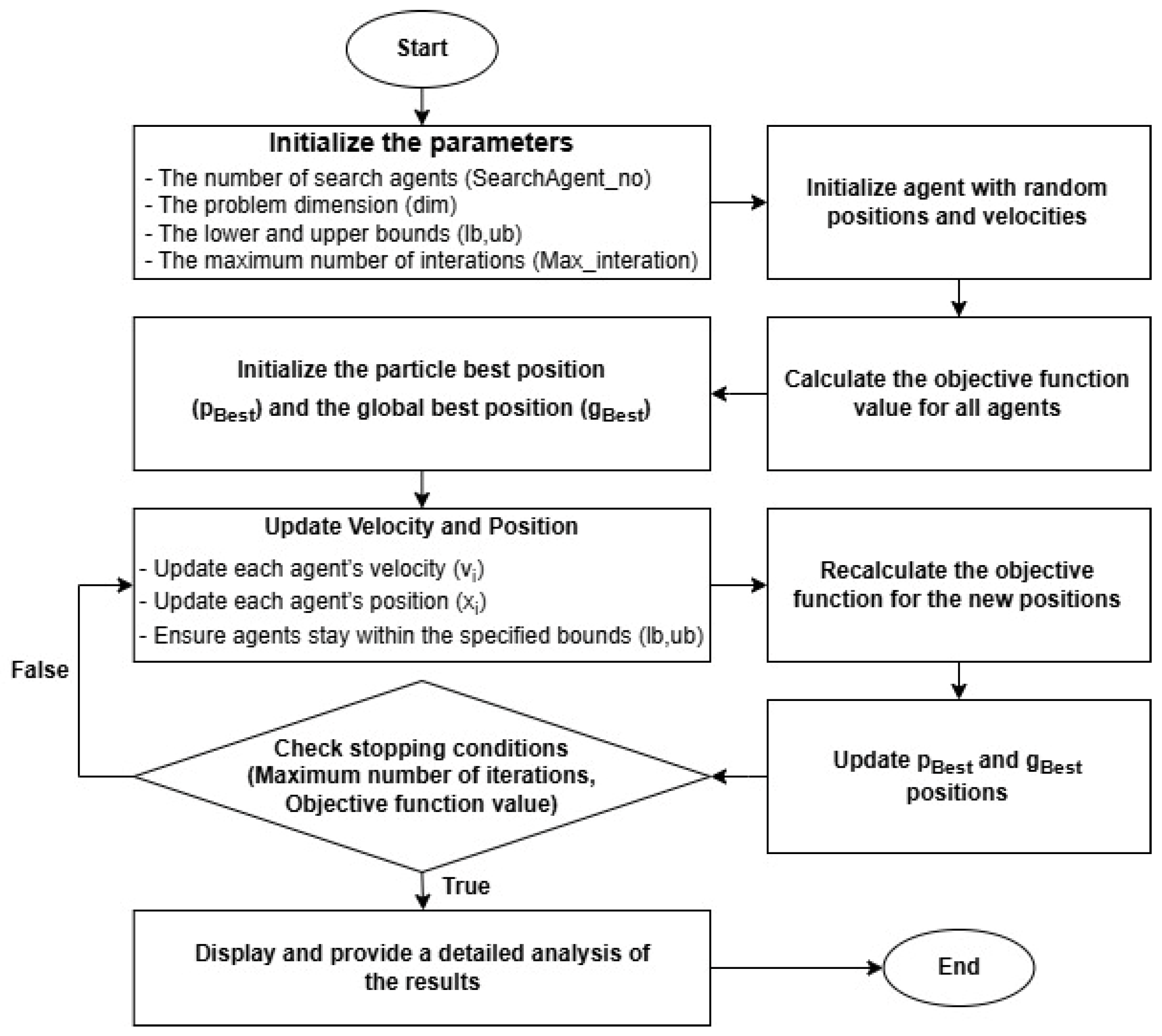
The PSO algorithm works by iteratively searching for the optimal solution. It starts with initializing a swarm of particles, each placed randomly within the search space and given random velocities. The fitness of each particle is then evaluated based on the objective function at its current position. Afterward, the algorithm updates each particle’s position and velocity according to specific formulas. As the process progresses, each particle keeps track of its own best position (pBest), and the swarm updates the global best position (gBest) accordingly. This cycle repeats until the algorithm meets a stopping condition, such as reaching a set number of iterations or finding a solution that meets the desired level of accuracy.

PSO offers several advantages, such as its simplicity, ease of implementation, and effectiveness in tackling a wide variety of optimization problems. One key benefit is that it does not require the calculation of gradients, which makes it especially useful for solving problems that are non-differentiable, nonlinear, or have multiple objectives. PSO also excels in global search, meaning it can explore the solution space efficiently and avoid getting stuck in local minima.

However, PSO is not without its challenges. The algorithm’s performance is highly dependent on the proper selection of parameters like w, c₁, and c₂, and fine-tuning these parameters for different problems can be time-consuming. In very large or complex search spaces, PSO may struggle and take longer to find the optimal solution. While PSO is effective in many situations, it does not always guarantee convergence to the global optimum and may occasionally settle for a local optimum too early.

The PSO algorithm is applied to various optimization problems across different fields, particularly in power systems. In frequency control systems, PSO can be used to optimize the parameters of PID controllers to adjust the generation power of power plants (such as hydropower and thermal power plants), thereby maintaining a stable frequency in the system. PSO helps to find optimal values for parameters like K_p, K_i, and K_d in PID controllers, aiming to minimize frequency errors and fluctuations when there are changes in consumption or generation power. Additionally, PSO is applied to optimize power distribution in multi-area power systems, helping to balance the load and minimize power generation costs. With its ability to efficiently search in complex solution spaces, PSO is a powerful tool for improving the stability and operational efficiency of power systems (Figure 1).

The optimization process requires a well-defined objective function to enhance frequency regulation effectively. In this study, the Integral of Time-weighted Absolute Error (ITAE) is chosen to guide the PSO-based tuning of PID controller parameters. ITAE prioritizes both rapid error minimization and system stability, making it a suitable criterion for LFC. The ITAE is mathematically defined as follows:

$$ITAE={\displaystyle \underset{0}{\overset{t_s}{\int }}{\displaystyle \sum _{i=1}^L(\left|\Delta f_i\right|+{\displaystyle \sum _{\begin{array}{c}j=1\\ i\ne j\end{array}}^L\left|\Delta P_{tie,ij}\right|}) tdt}}$$

(10)

where t_s is the overall duration of the simulation; and t is the time variable.

The ITAE metric serves as a key performance measure in optimizing PID controller parameters through PSO. By prioritizing the reduction in frequency deviation, overshoot, and settling time, ITAE ensures an improved dynamic response. The following simulation results will demonstrate its effectiveness through improved control accuracy and enhanced system stability across various conditions.

4. Simulation Results and Discussion

The simulation model employs a decentralized control approach, where individual PID controllers are assigned to power plants in each area to regulate and stabilize the system frequency. In the simulation scenarios, each PID controller is responsible for managing and adjusting the power output of its respective plant, ensuring that load variations and disturbances do not cause significant frequency fluctuations. The approach allows each plant to operate independently while maintaining overall system coordination.

This section explores the performance of frequency control strategies in multi-area power systems through the following three main scenarios:

• Scenario 1: A two-area power system integrating hydropower plants.
• Scenario 2: A three-area power system combining hydropower, reheat thermal, and non-reheat thermal power plants, with continuous load variations.
• Scenario 3: A three-area power system combining hydropower, reheat thermal, and non-reheat thermal power plants, with the integration of wind power.

These simulations aim to highlight how effective control strategies can ensure stable frequencies and efficient operations under varying load changes.

4.1. Scenario 1: A Two-Area Power System (TAPS) Integrating Hydropower Plants (Figure 2)

A load disturbance of 0.05 per unit (pu) is applied to the system at t = 1 s. The simulation runs for 30 s, providing sufficient time to analyze the frequency response and assess the effectiveness of the control strategy under varying load conditions.

To ensure accurate results and optimal system behavior, the simulation scenario was carefully designed with specific conditions and parameter values (

Table 1. Parameters for scenario 1.

Parameter	Unit	Value
B1 = B2	pu.MW/Hz	0.425
R1 = R2	Hz/pu.MW	2.4
Tgh1 = Tgh2	s	0.3
Trs1 = Trs2	s	5
Trh1 = Trh2	s	28.75
Tw1 = Tw2	s	0.3
Kps1 = Kps2	Hz/pu.MW	120
Tps1 = Tps2	s	20
T12	pu.MW/Hz	0.545

). The simulation was conducted with a swarm of 100 particles and a maximum of 50 iterations to balance computational cost and solution quality. A moderate inertia weight w of 0.5 was chosen to balance the exploration of new possibilities with the refinement of current solutions, thereby preventing early convergence. The influence of both pBest and gBest solutions was set equally, with acceleration coefficients c₁ and c₂ both at 1.5, to promote efficient convergence. Randomness, introduced through variables r₁ and r₂, helped to maintain diversity within the search and made the system less likely to get stuck in local optima. This parameter configuration was selected to allow the PSO algorithm to effectively tune the PID controller and achieve stable frequency regulation.

Figure 2. Model of frequency control system for two hydropower plants integration.

Figure 2. Model of frequency control system for two hydropower plants integration.

To evaluate the performance of the PID controller designed using the PSO algorithm, this paper compares it with a controller tuned using the traditional Ziegler–Nichols method. The comparison focuses on key performance metrics such as steady-state error and settling time, highlighting the strengths and trade-offs of each approach.

The Ziegler–Nichols method provides a systematic approach to tuning the parameters of a PID controller. The following are the steps to implement this method:

Step 1: Set the controller to Proportional-only (P) mode.

Set K_i = 0 and K_d = 0, keeping only K_p in the PID controller. This ensures that the system operates based solely on the proportional gain K_p.

Step 2: Determine K_u and T_u.

Gradually increase K_p in small increments until the system reaches the critical oscillation point, where the system response shows sustained oscillations with constant amplitude.

After determining the values of K_u and T_u, note that K_u is the value of K_p at the critical oscillation point, and T_u is the period of sustained oscillation.

Step 3: Calculate the PID parameters using the Ziegler–Nichols formula.

Using the values of K_u and T_u determined in Step 2, the Ziegler–Nichols formulas are applied to calculate the PID controller parameters, as follows:

$$\begin{array}{l}{K}_p=0.6K_u\\ K_i={\displaystyle \frac{2K_p}{T_u}}\\ K_d={\displaystyle \frac{K_p{T}_u}{8}}\end{array}$$

(11)

The parameters calculated using the Ziegler–Nichols method provide a basic tuning setup for the PID controller. However, this often leads to oscillatory or excessive responses and is not optimal for many complex systems.

The simulation results presented below highlight the performance comparison between the PSO-tuned PID controller and the Ziegler–Nichols PID controller (

Table 2. PID parameters for scenario 1.

Area	Method	Kp	Ki	Kd
1	PID-ZN	−2.7273	−1.9841	−0.9372
	PID-PSO	−6.5052	−8.5875	0.7574
2	PID-ZN	−2.7273	−1.9841	−0.9372
	PID-PSO	0.2876	−2.1088	−0.0644

). This analysis demonstrates the extent to which the PSO algorithm enhances system response compared to the traditional tuning method.

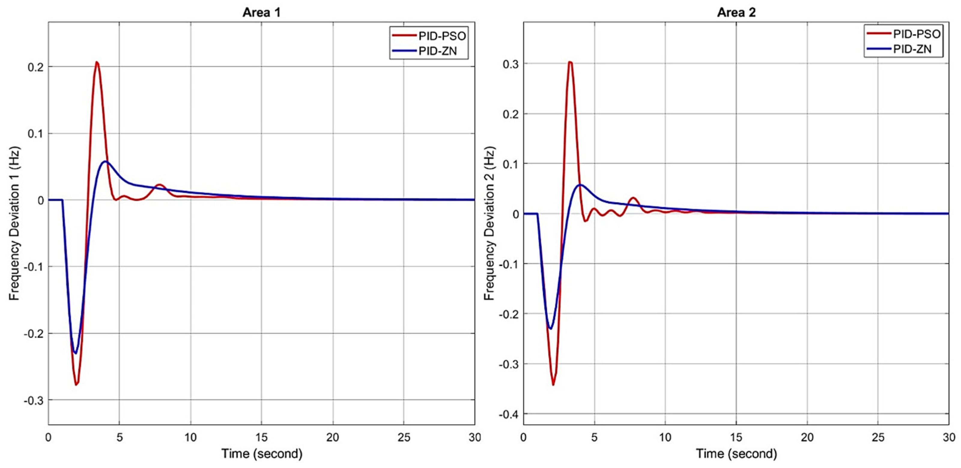
The two graphs depict the simulation results of a frequency control for two areas using two control methods, namely traditional PID-ZN and PID-PSO (combined with an optimization algorithm) (Figure 3). In the graph illustrating the results for area 1, the PID-ZN method shows that at 1 s, when a load disturbance of 0.05 pu is applied, the system frequency drops sharply to approximately −0.23 Hz at 3 s. It then suddenly rises to around 0.05 Hz and, in the subsequent period, the oscillation amplitude gradually decreases. By 18 s, the system frequency is adjusted to a balanced state. Meanwhile, the results of the PID-PSO method indicate that at 1 s, with the same load disturbance of 0.05 pu, the system frequency oscillates with a larger amplitude compared to the PID-ZN method by about 0.04 Hz. However, in terms of settling time, this method enables the system frequency to stabilize faster, achieving a steady state at 14 s. Similarly, for the frequency control results of area 2, the PID-PSO method once again outperforms the PID-ZN method. Although the initial oscillation amplitude is larger by approximately 0.1 Hz, the settling time is shorter, with 13 s compared to 18 s for the PID-ZN method. In both areas, the PID-PSO method demonstrates significantly smaller steady-state errors compared to the PID-ZN method. These results highlight the superiority of the PSO algorithm in optimizing PID parameters, which significantly improves frequency control performance, reduces settling time, and enhances accuracy in both areas (

Table 3. Comparison of simulation results for scenario 1.

Method	Area 1		Area 2
	Steady-State Error (Hz)	Settling Time (s)	Steady-State Error (Hz)	Settling Time (s)
PID-ZN	24.32 × 10−5	18	24.32 × 10−5	18
PID-PSO	6.973 × 10−5	14	6.969 × 10−5	13

).

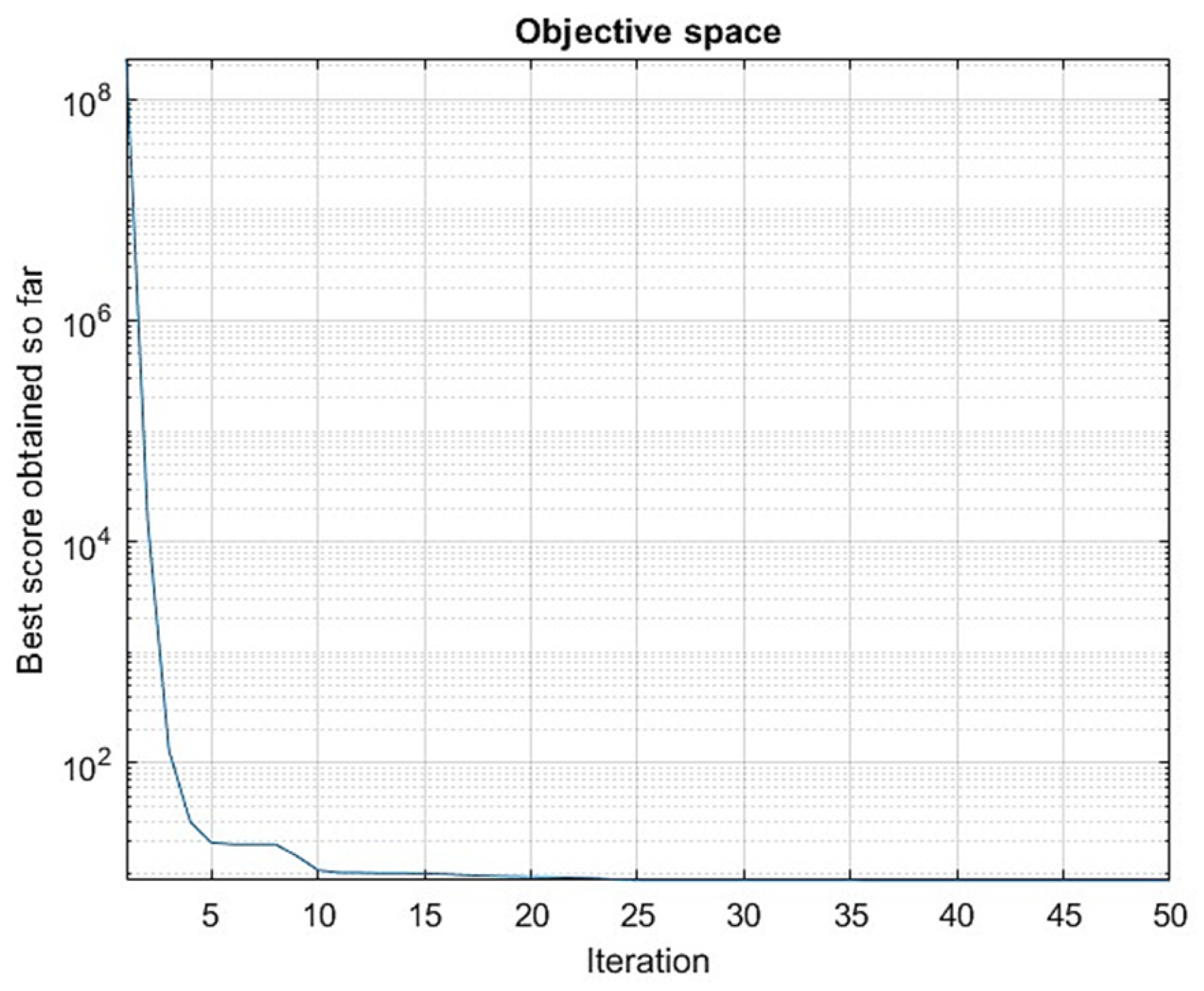
The convergence plot (Figure 4) shows the PSO algorithm’s effectiveness, with the objective function value dropping quickly. In the first five iterations, the value decreases from about 10⁸ to below 10², which indicates a substantial improvement in solutions early on. After that, the decrease slows down, and by the 24th iteration, the value stays nearly the same, showing that the algorithm has converged. This result suggests that the algorithm can reach a good solution in a short time while keeping the computation efficient.

Remark 1: The TAPS considered in this case has a more general structure compared to those presented in [4,19], which makes it more suitable for the application of LFC in real power systems.

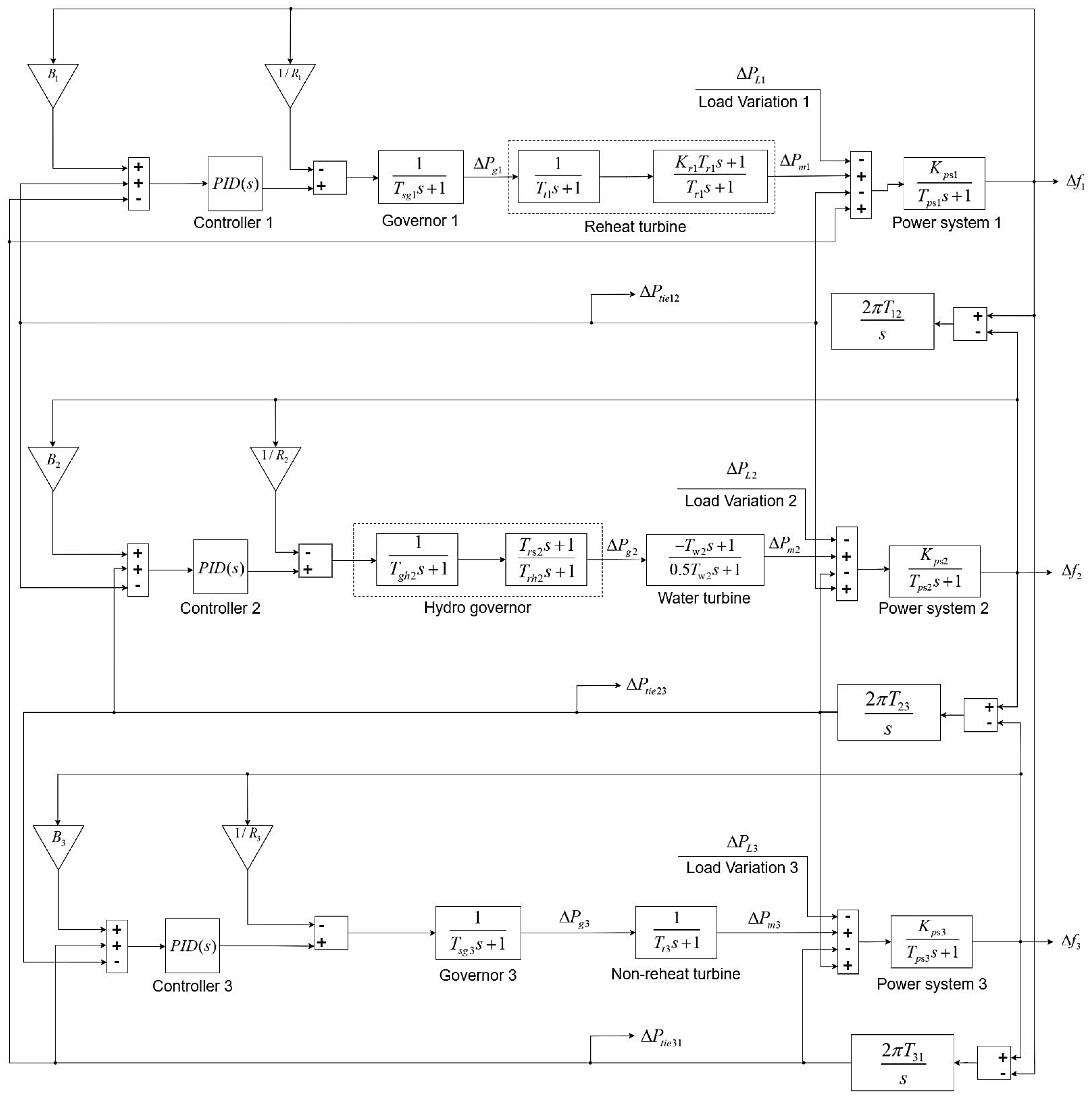
4.2. Scenario 2: A Three-Area Power System Combining Hydropower, Reheat Thermal, and Non-Reheat Thermal Power Plants, with Continuous Load Variations (Figure 5)

The comparison between the PSO-optimized PID technique and the traditional PID method, following the frequency regulation simulation for a two-area power system, clearly demonstrates the superior performance of the PSO algorithm. The PID-PSO controller not only balances the frequency more effectively but also achieves much faster stabilization. Building on these results, the study takes a step further by applying continuous load variations into a more complex system with the following three interconnected areas: a hydropower plant, a reheat thermal power plant, and a non-reheat thermal power plant. This extended simulation explores how well the PSO-optimized PID controller can uphold frequency stability and power balance across tie-lines. By analyzing the system’s dynamic responses to varying load conditions, the study offers valuable insights into the controller’s real-world practicality. It showcases its reliability and efficiency in complex power systems.

Figure 5. Model of frequency control system for hydropower, reheat, and non-reheat thermal power plant integration.

Figure 5. Model of frequency control system for hydropower, reheat, and non-reheat thermal power plant integration.

In this extended study, the simulation time will last for 60 s with a load that changes over time to mimic real-world conditions. To ensure consistency throughout the simulation process, the parameters set for the PSO algorithm remain unchanged for this scenario (

Table 4. Parameters for scenario 2.

Parameter	Unit	Value
B1 = B2 = B3	pu.MW/Hz	0.425
R1 = R2 = R3	Hz/pu.MW	2.4
Tsg1 = Tsg3	s	0.08
Tt1 = Tt3	s	0.3
Kr1	Hz/pu.MW	0.5
Tr1	s	10
Tgh2	s	0.3
Trs2	s	5
Trh2	s	28.75
Tw2	s	0.3
Kps1 = Kps2 = Kps3	Hz/pu.MW	120
Tps1 = Tps2 = Tps3	s	20
T12 = T23 = T31	pu.MW/Hz	0.545

). The load variation undergoes the following three distinct phases (Figure 6): from 1 to 20 s, the load gradually ramps up to 0.03 pu, much like the increased demand during peak hours. From 20 to 40 s, it increases to 0.05 pu, representing a period of consistently high demand, similar to heavy industrial usage or increased residential consumption. Finally, from 40 to 60 s, the load abruptly drops to 0.01 pu, illustrating situations where demand suddenly decreases, such as factory shutdowns or demand-side management initiatives. By continuously adjusting the load in this way, the research captures the unpredictable nature of real power systems. Moreover, it thoroughly tests how well the PSO-optimized PID controller can adapt and remain frequency stable under these fluctuating conditions.

Below are the simulation results for the continuous load variation scenario (

Table 5. PID parameters for scenario 2.

Area	Kp	Ki	Kd
1	−2.8563	−2.7593	−2.9135
2	−1.7872	−2.9356	−0.2980
3	−2.9861	−0.6005	−2.9815

), demonstrating the capability of the PSO-optimized PID controller to maintain frequency stability (Figure 7) and power balance between interconnected areas (Figure 8):

Overall, all three graphs (red, blue, and green) exhibit a similar trend in frequency variation. From 0 to 20 s, they show relatively large frequency fluctuations, with negative deviations ranging from −0.06 to −0.08 Hz, before gradually approaching a stable level (approximately 0 Hz). Moving into the 20–40 s interval, the frequency once again shows signs of fluctuation, this time ranging from about −0.04 to 0.05 Hz, before returning to a near-stable state. During the final 20 s of the simulation, all three graphs display their highest amplitude of frequency deviation, with positive deviations ranging from 0.08 to nearly 0.1 Hz. In summary, all three graphs indicate significant frequency fluctuations under load variations, yet they retain the ability to regulate and bring the frequency back to a stable state.

During the first 20 s, the red graph shows a few short-term positive peaks (around +0.01 to +0.02 pu) and slight dips (approximately −0.005 pu), generally oscillating around the 0 pu level. The blue graph remains relatively stable, fluctuating within ±0.01 pu, while the green graph exhibits even smaller deviations, ranging from ±0.005 to ±0.01 pu, indicating weaker load impacts on this branch. Between 20 and 40 s, the red and blue graphs display more significant variations, particularly near the 40 s mark, where the red graph drops below −0.02 pu, and the blue graph spikes to +0.02 pu before falling to around −0.02 to −0.03 pu. In contrast, the green graph maintains mild fluctuations, rarely exceeding ±0.01 pu. From 40 to 60 s, all three graphs experience pronounced swings around the 40 s point, then gradually recover toward the 0 pu level. While the red and blue graphs show minor ripples before stabilizing toward the end, the green graph maintains a lower amplitude of oscillation throughout.

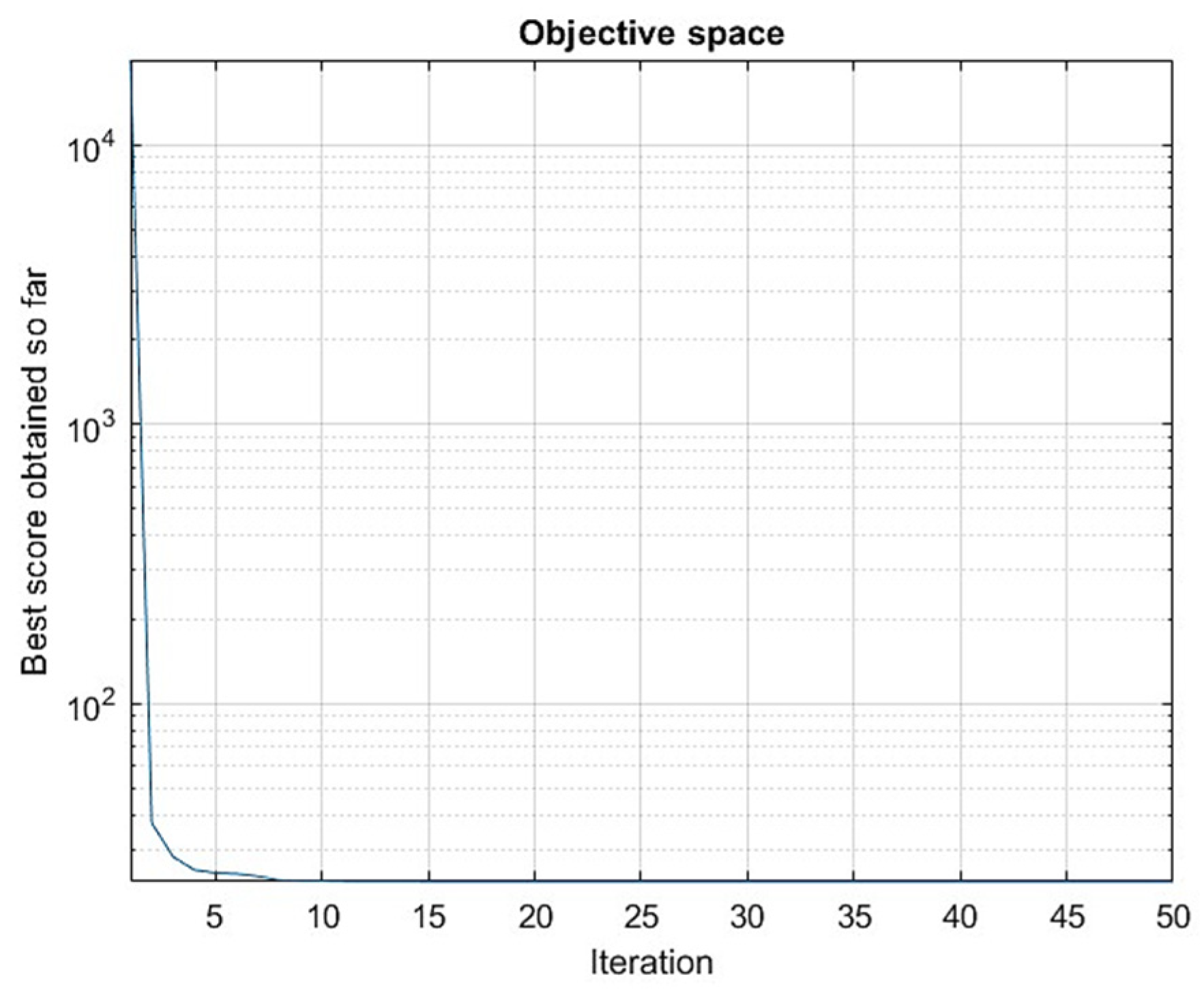
The convergence plot (Figure 9) demonstrates the performance of the PSO algorithm, where the objective function value drops rapidly within the initial iterations. As iterations progress, the rate of decrease slows down, and by approximately the eighth iteration, the value stabilizes, which means the algorithm has effectively converged. This behavior reflects the algorithm’s ability to find an optimal solution for the given optimization problem.

Remark 2: In contrast with the other approaches, the three-area power system combining the hydropower, reheat thermal, and non-reheat thermal power plants considered in this method has a more wide-ranging structure than the PS construction assumed in [12,17,18]. Furthermore, the proposed regulator built on PSO achieves better transient conditions in terms of zero frequency deviation error, small overshot, and settling time, which is useful to guarantee stability and reliability for the real PS.

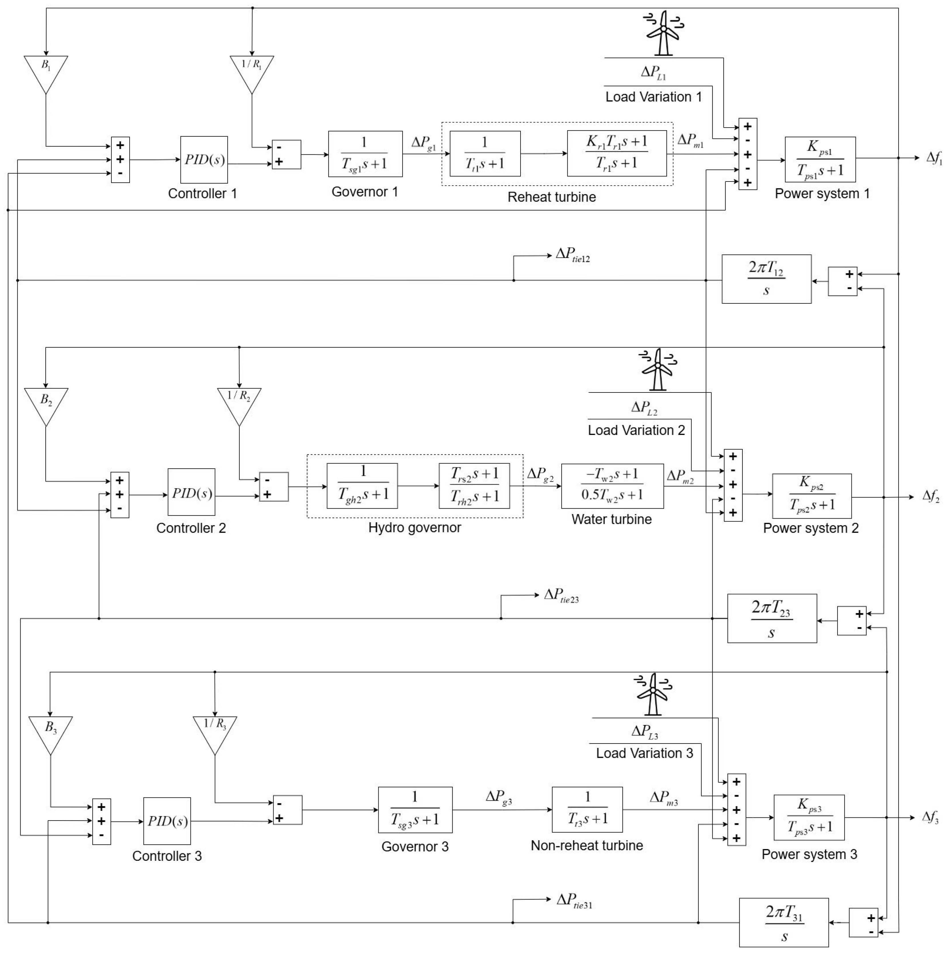
4.3. Scenario 3: A Three-Area Power System Combining Hydropower, Reheat Thermal, and Non-Reheat Thermal Power Plants, with the Integration of Wind Power (Figure 10)

In the third simulation scenario, the system still consists of three interconnected areas—a hydropower plant, a reheat thermal power plant, and a non-reheat thermal power plant. However, the key difference in this simulation is the integration of a renewable energy source, specifically wind power. Inspired by the study in [34], this scenario will examine the impact of wind speed variations on the output power of the wind energy system. This factor directly affects the frequency regulation and stability of the system.

The incorporation of renewable energy takes the research a step further, providing a more realistic perspective on the system’s ability to maintain frequency stability as more renewable energy sources are integrated. Through this simulation, the PSO-optimized PID controller will be evaluated more comprehensively. This assessment is particularly important under real-world operating conditions where wind energy fluctuations can significantly impact power balance and system frequency stability.

Figure 10. Model of frequency control system for hydropower, reheat, and non-reheat thermal power plant integration with wind power.

Figure 10. Model of frequency control system for hydropower, reheat, and non-reheat thermal power plant integration with wind power.

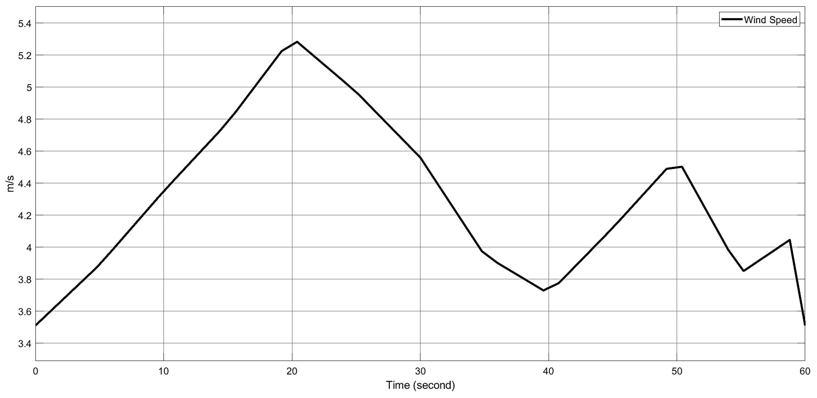
The parameters in the simulation model and the conditions for the PSO algorithm remain unchanged from Scenario 2. However, this simulation also incorporates wind power, requiring a wind fluctuation scenario. In this setup, wind speeds range from 3 m/s to 6 m/s, varying over time with random increases and decreases. These fluctuations help represent real-world wind conditions. The graph below shows how wind speed changes throughout the simulation (Figure 11).

With a total simulation time of 60 s, the load is set to fluctuate at 0.05 pu at the 1 s mark. The simulation is conducted, and the results are obtained as follows (

Table 6. PID parameters for scenario 3.

Area	Kp	Ki	Kd
1	−2.9374	−2.8921	−0.8143
2	−2.9457	−2.9763	−0.4858
3	−2.8532	−2.9016	−2.9845

):

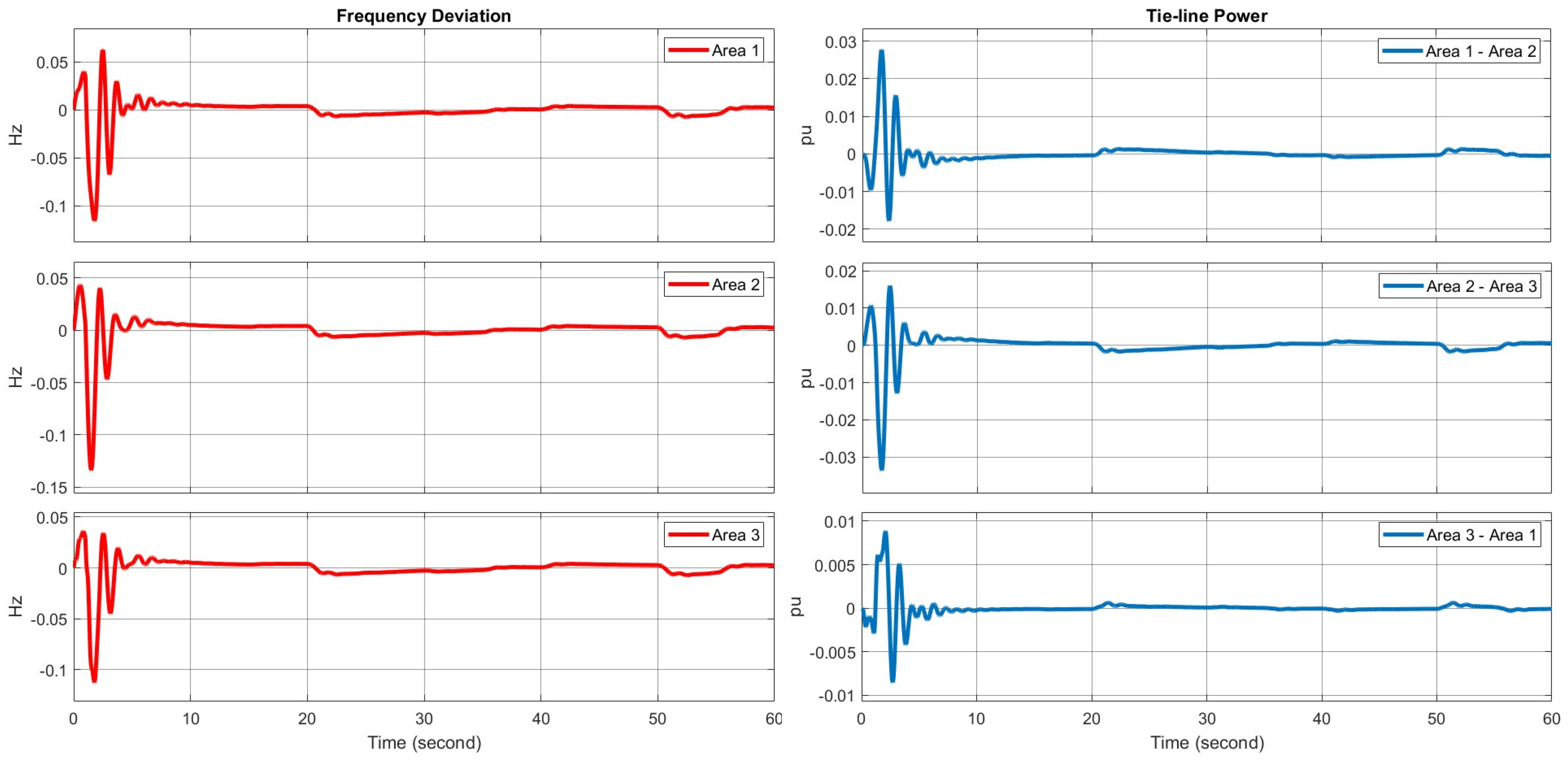
During the first 0–5 s, the frequency deviation of all three areas fluctuates significantly, with the maximum deviation reaching approximately −0.13 Hz, where area 2 experiences the largest deviation. The simulation scenario, which includes a load variation of 0.05 pu at 1 s, along with the integration of wind power with time-varying wind speeds, has led to strong oscillations in the initial phase. After t = 10 s, the frequency deviations gradually decrease and move towards a stable state. Around 50–60 s, the frequency deviation in all three areas fluctuates slightly around the equilibrium value, with an error of less than ±0.01 Hz, indicating that the system has been effectively regulated.

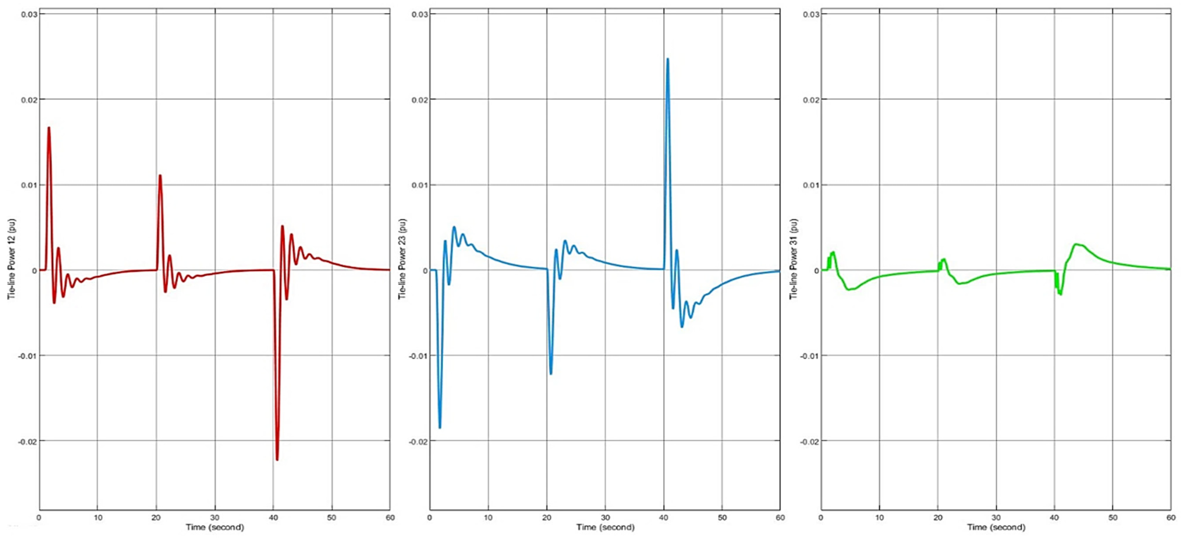
Regarding the tie-line power, during the first 5 s, power exchanges between the areas exhibit strong oscillations, particularly between areas 2 and 3, with an amplitude of approximately −0.032 pu. After t = 10 s, these fluctuations significantly decrease and gradually stabilize. From t = 50 s onward, tie-line power between the areas no longer exhibits major variations and remains stable with an error of less than ±0.002 pu. This demonstrates that the control algorithm has successfully balanced power among the areas, ensuring system stability (Figure 12).

The convergence plot (Figure 13) demonstrates the efficiency of the PSO algorithm, as the objective function value experiences a sharp decline during the initial iterations. Within the first five iterations, there is a significant decrease, indicating rapid progress in finding better solutions. By approximately the seventh iteration, the value stabilizes, signifying convergence. This pattern confirms the algorithm’s effectiveness in optimizing the given problem.

Remark 3: In contrast with the other approaches proposed in [9,15,23], the WP is integrated into the PS, which is used fully for the real PS. In addition, the simulation results reveal that the planned regulator built on PSO algorithm tuning remains suitable; subsequently, there are no fluctuations in the progression variable beforehand it spreads a steady state. This stay is exposed by the detail that the regulator output leads the WP through vacillation. This shows that the PID regulator, adjusted by algorithm expressions, has a fast and effective response to load changes and WP variations, which is beneficial in improving the performance of the PS.

5. Conclusions

In this paper, the results clearly demonstrate the effectiveness of using a PID controller combined with the PSO algorithm for frequency regulation in multi-area interconnected power systems, particularly in two-area and three-area systems. Simulation results highlight the ability of the PID-PSO method to regulate frequency fluctuations, significantly reduce frequency deviations, and shorten the stabilization time compared to the traditional PID-ZN method. In three-area systems, the PID-PSO method exhibits strong capabilities in maintaining frequency stability under continuously changing load conditions, further emphasizing the practical applicability of this study. These results underscore that integrating the PSO algorithm into PID parameter tuning not only enhances precision but also improves system resilience and performance under complex load fluctuation scenarios.

Although the PID-PSO method has proven to be effective, there are still many potential directions for further development. These include comparisons with other algorithms, such as GWO or WOA, or the application of hybrid approaches to fully leverage the strengths of each algorithm. Additionally, integrating artificial intelligence, such as deep learning and reinforcement learning, promises to significantly enhance PID parameter optimization, especially in nonlinear systems or systems integrating renewable energy sources. Practical experiments on power systems, combined with research on smart energy management, and load forecasting will be key to improving system performance and reliability.