An Enhanced TimesNet-SARIMA Model for Predicting Outbound Subway Passenger Flow with Decomposition Techniques

Abstract

The accurate prediction of subway passenger flow is crucial for managing urban transportation systems. This research introduces a hybrid forecasting approach that combines an enhanced TimesNet model, Seasonal Autoregressive Integrated Moving Average (SARIMA), and Variational Mode Decomposition (VMD) to improve passenger flow prediction. The method decomposes time series data into Intrinsic Mode Functions (IMFs) using VMD, followed by adaptive predictions for each IMF with TimesNet and SARIMA. The dataset spans from 1 January to 25 January 2019, encompassing 70 million records processed into five-minute intervals. The results show that the VMD preprocessing effectively extracts features, enhancing prediction performance (13.25% MAE, 19.7% RMSE improvements). The hybrid method excels during peak times (52.75% MAE, 50.61% RMSE improvements) and outperforms baseline models like Informer and Crossformer, achieving 66.14% and 63.24% improvements in the MAE and RMSE, respectively. This research offers a reliable tool for predicting subway passenger flow, supporting the smart evolution of urban transport systems.

1. Introduction

Rapid urbanization enhances the importance of subway systems in managing city traffic and improving commuter experiences. Accurate subway passenger flow forecasting is crucial for distributing transportation resources efficiently, reducing congestion, and planning future traffic networks. Subway passenger flow predictions utilize three main approaches: mathematical statistics, machine learning, and deep learning [1]. Our method enhances prediction accuracy by integrating elements from these established techniques. Although diverse prediction techniques aim to improve the accuracy of subway passenger flow forecasts, the complex and dynamic nature of these data presents significant challenges. These techniques struggle to capture deep-level data, impacting the precision and reliability of forecasts.

Conventional mathematical statistical approaches like the Autoregressive Integrated Moving Average (ARIMA) [2] are popular in subway passenger flow forecasting due to their simplicity and ease of use. However, their effectiveness is limited when dealing with complex, non-smooth traffic flow data, often leading to poor outcomes. In response, researchers have turned to machine learning methods such as SVM, decision trees, and random forests [3,4,5], which offer improved data processing and pattern recognition capabilities, enhancing prediction accuracy and leading to advancements in predictive models. Despite their advancements, these machine learning models require extensive feature engineering and struggle with long-term dependencies and seasonal variations in time series data [6], limiting their effectiveness. Concurrently, more sophisticated deep learning techniques like Convolutional Neural Networks (CNNs) and Recurrent Neural Networks (RNNs) [7,8,9,10] have been broadly utilized for forecasting subway passenger flow. Recent advancements in subway passenger flow prediction have utilized a range of methods, from traditional ARIMA/SARIMA models to more complex deep learning approaches such as LSTM and Transformer-based architectures. These models have shown varying degrees of success in addressing the nonlinear and time-varying nature of passenger flow data. However, many face challenges such as scalability, interpretability, and computational cost [11,12].

To enhance the effective extraction of various types of information from raw traffic data, various methods for transforming time series data into frequency domain components have been widely applied to passenger flow data, road traffic flow data, and other types of time series data. Fourier transform is one such method, and empirical mode decomposition (EMD) proposed by NE Huang and others can decompose time series data into a few Intrinsic Mode Functions (IMFs) and a residue term [13]. Analyzing these components enables the extraction of the deep features of the sequence data at different time scales. Wu et al. employed the empirical mode decomposition and reinforcement learning techniques to predict short-term passenger flow in urban rail transit systems [14]. The model effectively enhanced the accuracy of the predictions. However, the process of EMD suffers from issues such as end effects and mode mixing, which can lead to the omission of valuable information and affect the decomposition accuracy. EEMD, CEEMDAN, and ICEEMDAN have addressed some of the limitations of the original EMD by reducing mode mixing and improving signal decomposition stability [15,16,17]. Sun et al. used a wavelet model to decompose subway passenger flow data into low-frequency and high-frequency components to provide more accurate information extraction, but the type of wavelet limits its accuracy. Classical frequency models, such as Fourier transforms, struggle to capture non-stationary data characteristics. Wavelet transforms, while effective in decomposing non-stationary data, have limitations in selecting an appropriate wavelet basis and in capturing complex nonlinear relationships [18]. While EWT is more versatile due to its ability to customize the transformation based on signal characteristics, VMD was selected in this study because it offers better control over the decomposition of specific frequency components. This makes it highly effective for handling complex and noisy subway passenger flow data, where the accurate separation of frequency components is critical [19,20,21,22,23].

Overcoming the shortcomings of current methods in the research process poses a significant challenge in the area of subway passenger flow forecasting. The latest research trend involves the effective improvement and proper integration of mathematical statistics methods, machine learning, and deep learning approaches, exploiting the advantages of each model while avoiding their risks and drawbacks [24]. The primary benefit of enhancing diverse models for subway passenger flow data is their targeted approach; they can analyze and forecast from various perspectives, considering the “non-stationary” and “seasonal” attributes of subway passenger flow data [25,26,27,28,29]. For instance, the SARIMA model and TimesNet model, although they are mathematical statistics and deep learning models, respectively, can model time series targeting the “seasonality”, “smoothness”, and “intra-period” and “inter-period” characteristics of passenger flow data. In light of the above models’ characteristics, this paper proposes an improved TimesNet subway passenger flow prediction model based on Multi-scale Variational Mode Decomposition (VMD) and the incorporation of a seasonal module. The model decomposes subway passenger flow data via VMD into IMFs of various frequencies, then feeds these decomposed IMFs into the improved TimesNet model with a seasonal module for prediction and, finally, reconstructs the predicted outcome. In our proposed method, judging from the seasonal detection module, the SARIMA component is primarily responsible for capturing the linear trends and seasonal variations in subway passenger flow data, while the improved TimesNet parallel is tasked with capturing and simulating the nonlinear patterns and complex “within-period” and “across-period” dependencies of subway passenger flow data [30]. Such targeted improvements, tailored to the characteristics of subway passenger flow data, can effectively enhance the accuracy of subway passenger flow predictions. Meanwhile, it is important to clarify that the “seasonal variations” referred to in this study specifically address short-term seasonality. In the context of subway passenger flow data, this refers to recurring patterns observed within a single day, such as the morning and evening rush hours, as well as the differences between weekdays and weekends. These short-term cycles are critical for understanding and optimizing subway operations, as they provide valuable insights into passenger flow fluctuations throughout the day and week.

The experiments conducted in this paper selected real swipe card data from the Hangzhou subway in 2019 (a total of 70 million records) and processed them to produce subway passenger flow data with a time step of five minutes. In time series analysis, especially for complex urban transportation systems, it is crucial to account for both linear and nonlinear dynamics. While linear models such as SARIMA are effective at capturing the seasonal and trend components of the data, many real-world systems, including metro passenger flow, exhibit nonlinear and chaotic behavior. Nonlinear dynamics can be identified through various metrics such as the Lyapunov exponent, correlation dimension, and pseudo-attractor analysis [31,32]. In this paper, we verify the nonlinearity and chaotic nature of the dataset time series by analyzing them as described above.

The results demonstrate that our method shows significant performance improvements over other baseline models (e.g., Autoformer, TimesNet, Crossformer) in terms of the Mean Absolute Error (MAE) and Mean Squared Error (MSE) evaluation metrics. In the model rationalization in our method section, the presented results reveal the impact of incorporating the improved TimesNet model, the SARIMA module, and the VMD module on the final model metrics, further validating the rational scientific basis of our prediction model. While the primary focus of this study is on predicting subway passenger flow, the proposed hybrid SARIMA-TimesNet model is designed as a versatile time series prediction framework. Due to its ability to effectively capture both linear and nonlinear components, the model can be applied to a wide range of domains that exhibit complex temporal patterns. For instance, in the energy sector, the model could be used to forecast consumption trends or electricity demand by accounting for both seasonal fluctuations and unexpected surges. In financial markets, it could help predict stock prices, exchange rates, or market indices by modeling inherent volatility and cyclical behavior. Moreover, in meteorology, the model could assist in predicting weather patterns by capturing recurring seasonal shifts and abrupt changes. These examples underscore the adaptability and robustness of the SARIMA-TimesNet model, making it suitable for any field where time series data involve a combination of predictable cycles and irregular variations.

The structure of this paper is outlined as follows: The passenger group prediction model for subway flow data, tailored to their characteristics, will be described in detail in Section 2; Section 3 will compare the experimental results of various models and analyze the functionality of each block in our proposed method; Section 4 will provide a conclusive summary; and the final section will discuss future research directions.

2. Methodology

2.1. Overall Model Framework

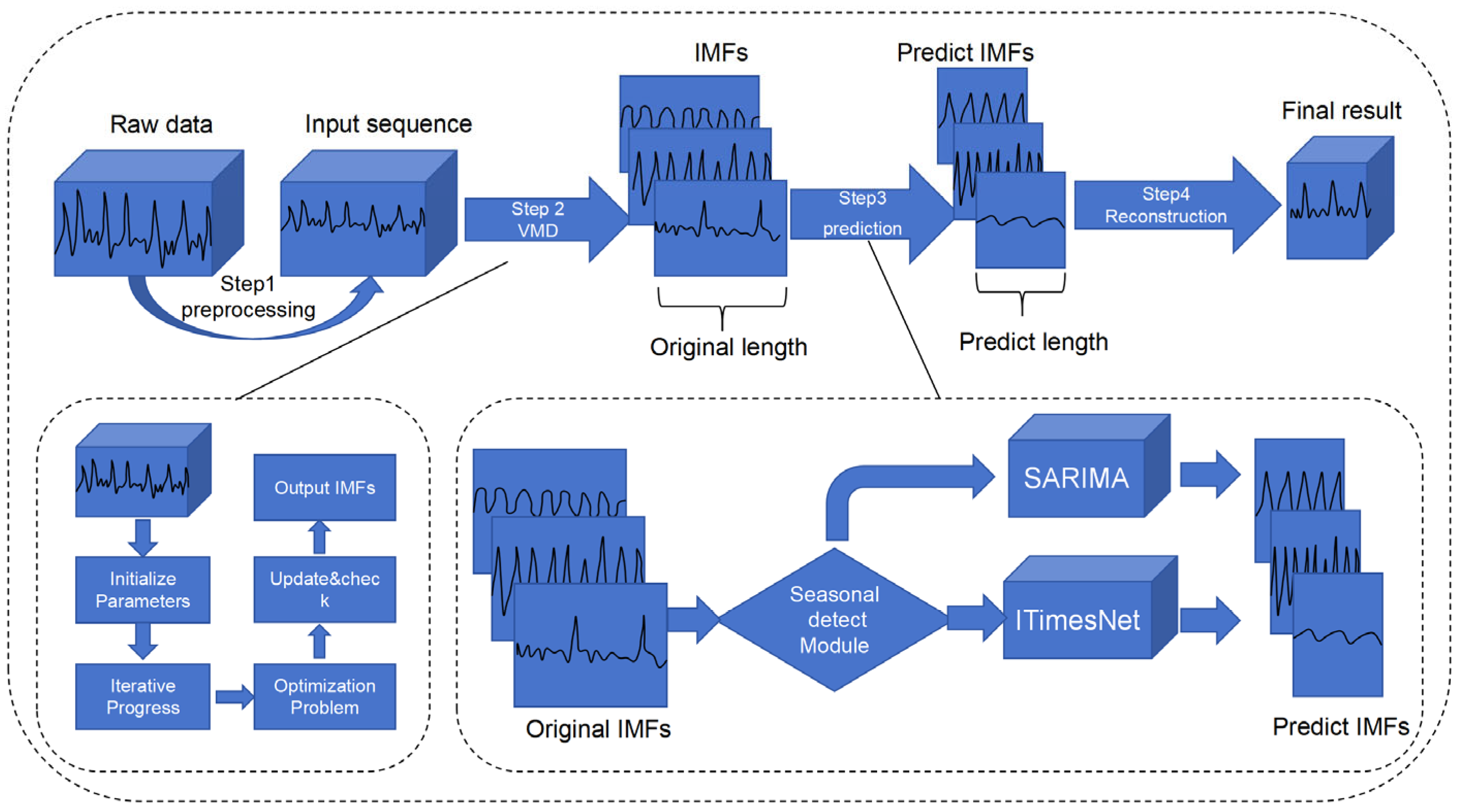
Figure 1 shows the model framework described in this paper. As illustrated in Figure 1, the overall operation process of this prediction model follows these 4 steps:

(1) Data Preprocessing: initially, the raw data undergo zero-padding operations and normalization to yield a cleaned dataset, which serves as the original input sequence.

(2) Variational Mode Decomposition (VMD): The cleaned dataset is then subjected to VMD to extract the corresponding Intrinsic Mode Functions (IMFs), obtaining a set of n IMFs. The VMD process involves iterative parameter initialization, optimization, and the update and check mechanism to produce the final IMFs.

(3) IMF Prediction: the obtained IMFs are standardized using the following formula:

$${IM{F}^{\prime }}_i={\displaystyle \frac{{IM{F}^{\prime }}_i-{IMF}_{i}min}{{IMF}_{i}max-{IMF}_{i}min}}$$

(1)

Each of the resulting IMFs is then fed into a seasonality detection module. This module utilizes the autocorrelation function (ACF) and partial autocorrelation function (PACF) to identify IMFs with significant seasonal characteristics [33,34]. The IMFs exhibiting strong seasonality are input into the SARIMA model, while those without strong seasonality, which exhibit stronger nonlinear and non-periodic patterns, are directed to an improved TimesNet model.

(4) Reconstruction: Finally, after each IMF has been predicted through either SARIMA or TimesNet, all the predicted components are reconstructed to generate the final prediction. This reconstruction step is essential because the VMD decomposes the original sequence into several IMFs, and reconstructing these predicted IMFs allows for the restoration of the overall predicted sequence [35]. This comprehensive framework captures both strong seasonal components and nonlinear features in the data, thus effectively utilizing all the available information for accurate prediction outcomes.

In this paper, a dataset constructed from real passenger flow data of the Hangzhou subway is used, and the sliding window technique is applied for forecasting. The data are segmented into five-minute intervals, with a total of 232 time steps in a day (covering the data within the statistics time), which serves as the length of the forecasting window (the sliding window length). Additionally, the sliding window can be adjusted based on experimental requirements. For each day forecasted, the window slides by 232 time steps, and the actual values from the previous day are used to update the dataset.

As shown in Figure 2, we utilized sliding windows of 232 time steps (a full day) to capture passenger flow patterns over different time horizons.

Similarly, the prediction of each component obtained after Variational Mode Decomposition (VMD) also employs the sliding window concept. A detailed description of the VMD module and improved TimesNet model as well as the SARIMA model will be provided in the subsequent sections.

2.2. VMD Module

Variational Mode Decomposition (VMD), first introduced in 2014 by Dragomiretskiy and Zosso, is a technique used to decompose nonlinear, non-stationary data into multiple Intrinsic Mode Functions (IMFs), separating the local characteristics of the data [36]. VMD decomposes the time series data into Intrinsic Mode Functions (IMFs), each representing a different frequency component. High-frequency IMFs capture short-term fluctuations, while low-frequency IMFs reveal long-term trends. This decomposition helps to isolate noise and enhance the detection of underlying periodic patterns, improving the accuracy of passenger flow predictions. The criteria for identifying an IMF can be summarized as follows:

(1) The number of extrema and the number of zero-crossings must differ at most by one throughout the entire sequence;

(2) At any point, the mean of the envelope defined by the local maxima and the envelope defined by the local minima is zero.

VMD serves as a key step in the subway passenger flow prediction model proposed in this paper. The VMD of a signal $X$ can be represented as follows:

$$X={\sum }_{k=1}^K{u}_k\left(t\right)$$

(2)

where ${\mathrm{u}}_{\mathrm{k}}\left(\mathrm{t}\right)$ are the IMFs, and k represents the number of Intrinsic Mode Functions.

The purpose of VMD is to decompose complex subway passenger flow data into a finite set of IMFs, which each represent different frequency components. These IMFs are then used to reveal deeper characteristics of the subway passenger flow data. The objective of VMD is to minimize the bandwidth of the IMFs by solving the following optimization problem:

$${min}_{\left\{u_k\right\}}{\sum }_{k=1}^K‖{\partial }_t\left[{\left(u_k\left(t\right)-{\widehat{u}}_k\left(t\right)\right)}^2\right]‖$$

(3)

where ${\widehat{u}}_k\left(t\right)$ are the Hilbert transforms of the IMF ${\widehat{u}}_k\left(t\right)$, and the operator ${\partial }_t$ refers to the partial derivate with respect to time. The Hilbert transform is used for the instantaneous frequency analysis of the decomposed Intrinsic Mode Functions (IMFs), allowing for a more accurate capture of the nonlinear characteristics in the data. The optimization problem aims to minimize the total bandwidth of the IMFs by solving this equation iteratively. This ensures that the IMFs generated are as narrowband as possible, capturing distinct frequency components from the signal.

In VMD, each IMF is modeled as a mode function $u_k\left(t\right)$ that is the output of a bandpass filter with a fixed center frequency ${\omega }_k$. The mode function can be expressed as follows:

$$u_k\left(t\right)=A_k\left(t\right)cos\left({\varphi }_k\left(t\right)\right)$$

(4)

where $A_k\left(t\right)$ is the amplitude envelope, and ${\mathsf{\varphi }}_k\left(t\right)$ is the instantaneous phase.

VMD is a non-recursive, adaptive, and data-driven method that can decompose nonlinear and non-stationary data into IMFs with limited bandwidth. The center frequencies ${\omega }_k$ and bandwidths are iteratively updated by solving the constrained optimization problem to ensure accurate decomposition.

The parameters of these mode functions, including their center frequencies and bandwidths, are determined by solving a constrained optimization problem that minimizes the bandwidth of each IMF and makes their sum as close as possible to the original signal.

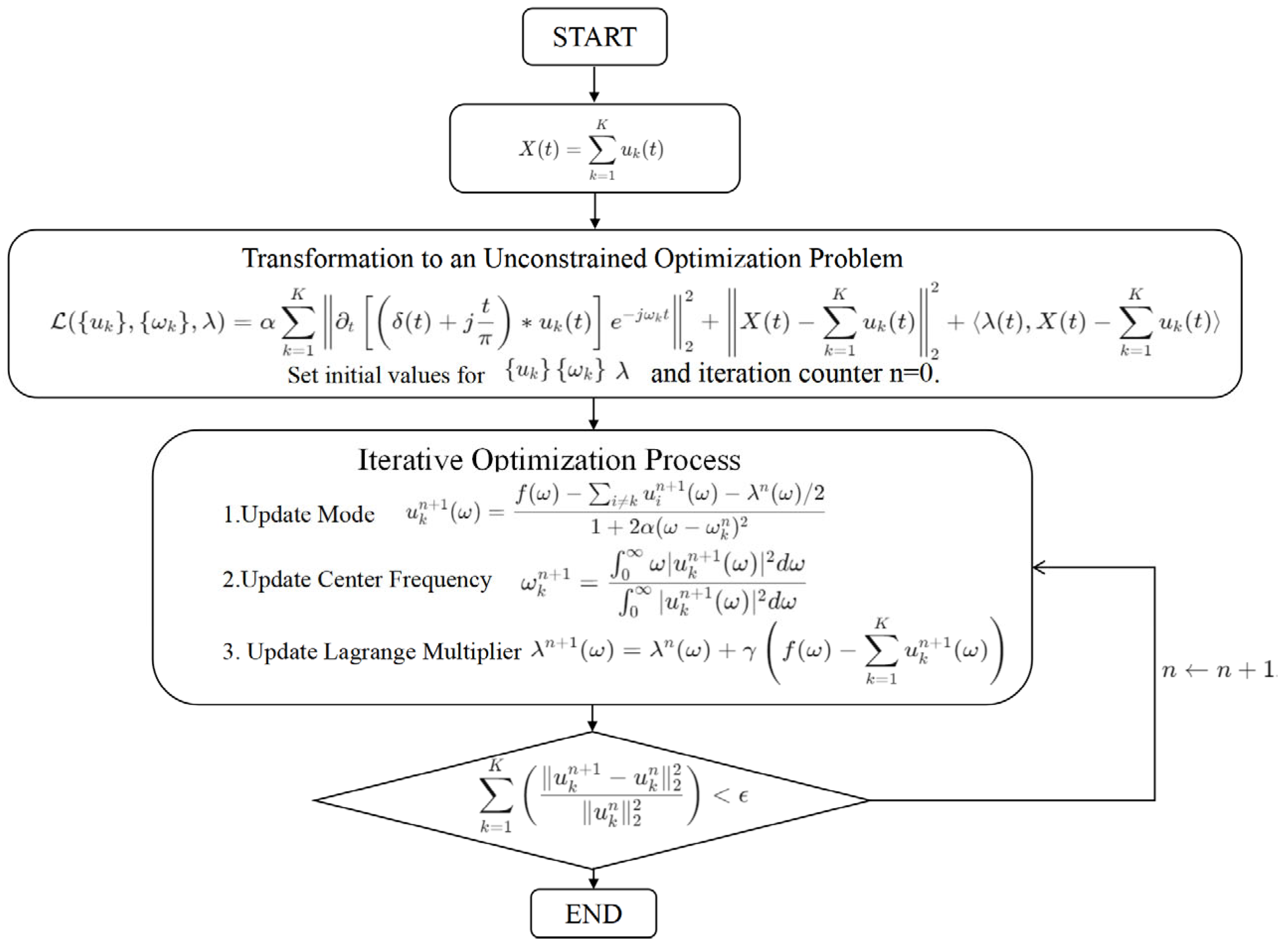
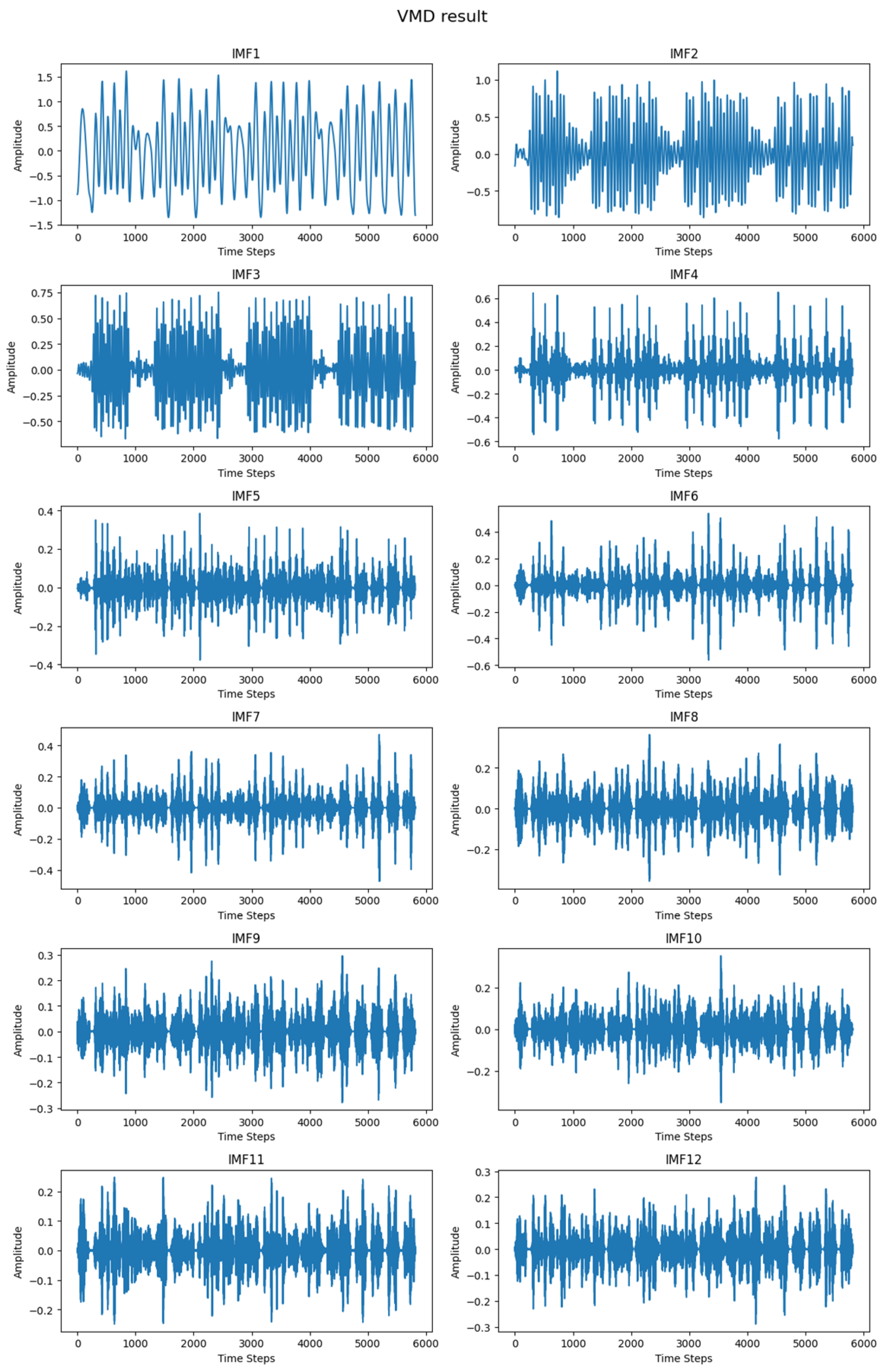
As shown in Figure 3, the VMD module in this paper executes the following steps:

Step 1: Data Preprocessing. The original metro passenger flow data are normalized to ensure consistent scaling, reducing the influence of different data scales on the analysis and aiding convergence in subsequent optimization. The preprocessed data $X\left(t\right)$ are input into the VMD module, where they are first transformed into a variational optimization problem. The original time series $X\left(t\right)$ can be represented as follows:

$$X\left(t\right)=\sum _{k=1}^K{u}_k\left(t\right)$$

(5)

Step2: Transformation to an Unconstrained Optimization Problem. The augmented Lagrangian function for VMD is formulated to minimize the bandwidth of the Intrinsic Mode Functions (IMFs) while constraining the sum of all IMFs to

$$\mathcal{L}\left(\left\{u_k\right\},\left\{{\omega }_k\right\},\lambda \right)=\alpha \sum _{k=1}^K{∥{\partial }_t\left[\left(\delta \left(t\right)+j{\displaystyle \frac{t}{\pi }}\right)\ast u_k\left(t\right)\right]e^{-j{\omega }_{k}t}∥}_2^2+{\left|\right|X\left(t\right)-\sum _{k=1}^K{u}_k\left(t\right)\left|\right|}_2^2+⟨\lambda \left(t\right),X\left(t\right)-\sum _{k=1}^K{u}_k\left(t\right)⟩$$

(6)

Here, $\alpha$ represents the penalty parameter, and $\lambda \left(t\right)$ is the Lagrange multiplier used to ensure that the sum of all IMFs matches the original time series.

Step 3: Iterative Optimization Process. A dual optimization strategy is used to iteratively update the estimation of modes $u_{k^{\prime }}$ their center frequencies ${\omega }_k$, and the Lagrange multiplier $\lambda$ until the solution converges.

Step 3.1: Initialization. $\left\{u_k\right\},\left\{{\omega }_k\right\},\lambda$ is initialized, and the iteration counter $n=0$ is set.

Step 3.2: Iterative Updates and Convergence Check. For each iteration $n$, the following updates are performed:

1. Mode $u_k^n+1\left(\omega \right)$ is updated:

$$u_k^{n+1}\left(\omega \right)={\displaystyle \frac{f\left(\omega \right)-\sum _{i\ne k}{u}_i^{n+1}\left(\omega \right)-\frac{{\lambda }^n\left(\omega \right)}{2}}{1+2\alpha {\left(\omega -{\omega }_k^n\right)}^2}}$$

(7)

Here, $f\left(\omega \right)$ represents the Fourier transform of the original signal.

2. The center frequency ${\omega }_k^{n+1}$ is updated:

$${\omega }_k^{n+1}={\displaystyle \frac{{\int }_0^{\mathrm{\infty }}\omega {\left|u_k^{n+1}\left(\omega \right)\right|}^{2}d\omega }{{\int }_0^{\mathrm{\infty }}{\left|u_k^{n+1}\left(\omega \right)\right|}^{2}d\omega }}$$

(8)

This update helps estimate the central frequency of each mode to ensure that it accurately captures the frequency characteristics of the IMF.

Step 3.3: The Lagrange multiplier ${\lambda }^{n+1}$ is updated:

$${\lambda }^{n+1}\left(\omega \right)={\lambda }^n\left(\omega \right)+\gamma \left(f\left(\omega \right)-\sum _{k=1}^K{u}_k^{n+1}\left(\omega \right)\right)$$

(9)

The parameter $\gamma$ controls the adjustment of the Lagrange multiplier, aiding in the convergence of the solution. Convergence check: after each iteration, it is checked whether the solution has converged by evaluating the relative change:

$$\sum _{k=1}^K\left({\displaystyle \frac{\parallel u_k^{n+1}-u_k^n{\parallel }_2^2}{\parallel u_k^n{\parallel }_2^2}}\right)<ϵ$$

If the convergence criterion is met, the process terminates; otherwise, $n$ is incremented, and the process continues.

Step 4: Extraction of IMFs. The output consists of $K$ IMFs $u_k\left(t\right)$ that collectively represent the original signal. These IMFs are the core components that highlight different intrinsic frequency bands of the time series data, making the signal analysis more interpretable and effective for further modeling.

The VMD algorithm effectively deconstructs complex signals into simpler components that can be analyzed and modeled more easily. In the context of subway passenger flow forecasting, this decomposition allows for a refined analysis of the data’s inherent features, such as daily patterns, peak periods, and anomalies, thereby enhancing the forecasting model’s ability to capture and predict future trends based on historical data.

2.3. Seasonal Detection Module

In the previous section, this paper provided a comprehensive introduction to the VMD process. In the following section, we will elaborate on the seasonal detection model tailored for choosing the appropriate IMFs in subway passenger flow prediction.

Therefore, the model proposed in this article will first input the decomposed sequence data into the “seasonal detection” module to determine if they have strong seasonal characteristics (the specific algorithm in the seasonal detection module is described in detail in the Supplementary Materials).

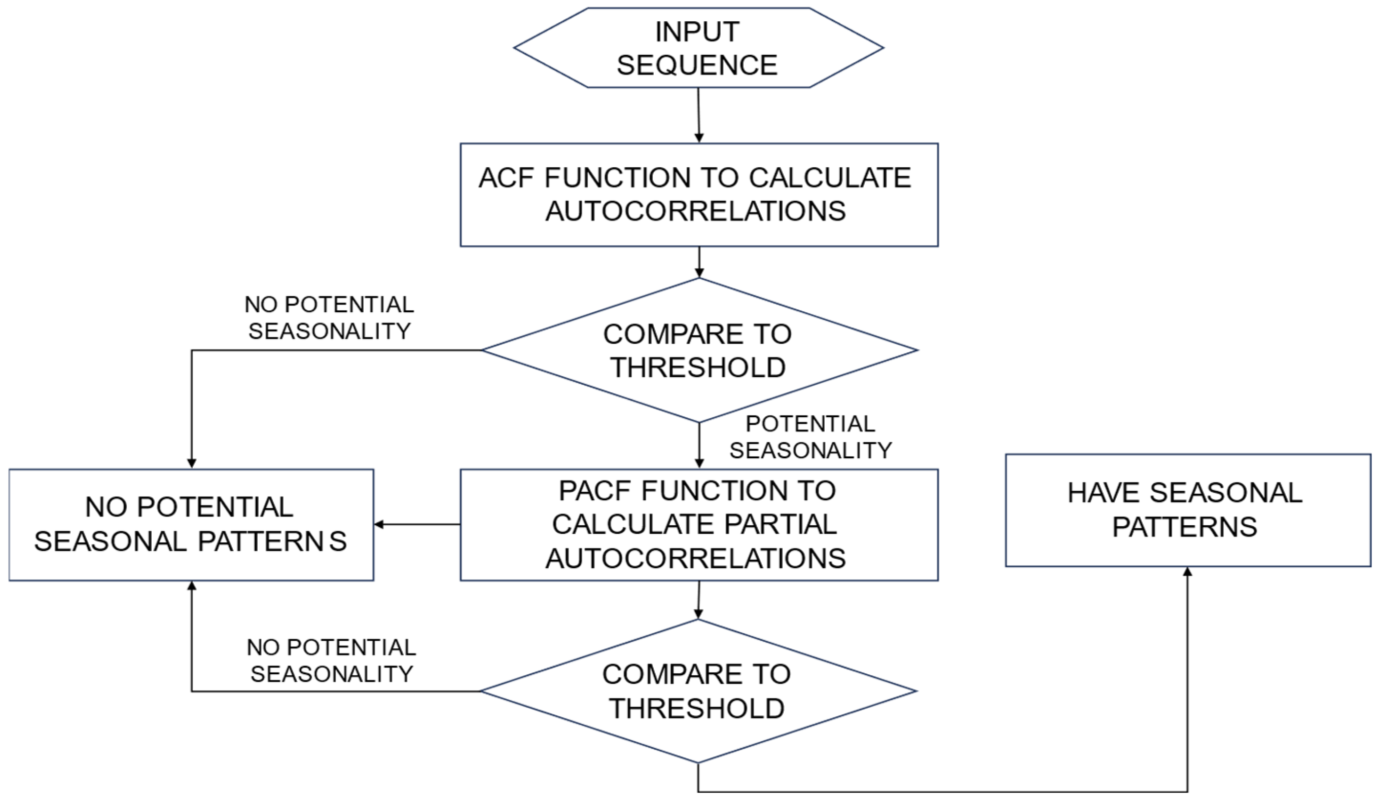
As illustrated in Figure 4 the seasonality detection module introduced in this study initially receives sequences of Intrinsic Mode Functions (IMFs) as input. It then calculates the autocorrelation function (ACF) to assess the correlation between the time series.

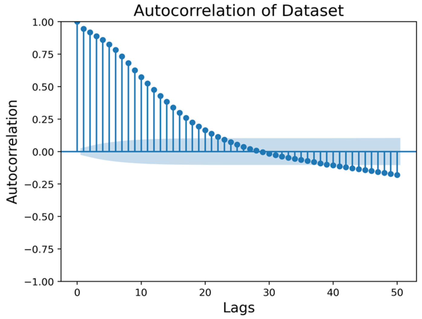
The autocorrelation function (ACF) measures the correlation between observations of a time series that are separated by a specific time lag. The ACF also helps to identify the direct impact of a specific lag on the current observation, independent of the influence of intermediate lags. It provides insights into how past values influence future values.

Series X and its lagged versions are described by the following equation:

$$ACF\left(k\right)={\displaystyle \frac{{\sum }_{t=1}^{n-k}\left(X_t-\overline{X}\right)\left(X_{t+k}-\overline{X}\right)}{{\sum }_{t=1}^n{\left(X_t-\overline{X}\right)}^2}}$$

(10)

Equation (10) quantifies the autocorrelation between the time series $X$ and its lagged version. Specifically, it calculates the relationship between the series value $X_t$ and the lagged series $X_{t+k}$ for a given lag $k.$ This equation helps determine whether significant seasonality exists, providing a basis for seasonal analysis in time series.

The ACF values obtained are compared with a predetermined threshold, set at 0.9 for this study. This threshold was selected as a balance between detecting significant correlations and minimizing false positives. A higher threshold, such as 0.95, might be overly restrictive and risk missing relevant seasonal patterns, while a lower threshold could introduce noise, falsely identifying non-seasonal fluctuations as significant. By choosing 0.9, we ensure that only meaningful seasonal trends are detected, allowing for reliable analysis. However, we recognize that the choice of threshold may influence the detection of seasonality, and further exploration of optimal threshold values will be an important focus in future research. If the ACF values exceed this threshold, the module proceeds with further analysis by calculating the partial autocorrelation function (PACF) of the series to confirm the presence of seasonality. The partial autocorrelation function (PACF) measures the correlation between an observation and its lagged value while controlling for the correlations at all shorter lags. This helps to identify the direct impact of a specific lag on the current observation, independent of the influence of intermediate lags.

Specifically, the calculation of PACF values can be expressed as follows:

$$PACF\left(k\right)=Cov\left(X_t,X_{t+k}|X_{t+1},\cdots ,X_{t+k+1}\right)$$

(11)

Here, $Cov$ denotes the covariance given the intermediate variables. The PACF is computed using statistical software to measure the correlation between the series and its lagged versions, excluding the effects of intermediate lags. If the PACF value surpasses the 90% confidence interval, it is interpreted as an indication of significant seasonality. Should the series not exhibit significant seasonality in either the ACF or PACF assessments, the module will conclude the absence of seasonality in the series.

The framework of the seasonal detection model is illustrated in Figure 4.

Then, adaptively, the appropriate IMFs (Intrinsic Mode Functions) are inputted into the corresponding improved TimesNet and SARIMA (Seasonal Autoregressive Integrated Moving Average) modules.

2.4. Improved TimesNet Module

Subway passenger flow prediction inherently requires time series forecasting. Recent studies have seen a surge of prediction methodologies based on Transformer model variants, such as the Informer model composed of multi-head self-attention mechanisms and the Autoformer model that involves decomposing and then forecasting sequences before recombining data. These models have provided theoretical support for modeling subway passenger flow data prediction in this paper.

In ICLR 2023 (a prominent academic conference in the field of machine learning and AI), the TimesNet model composed of multiple “Timesblock” modules emerged as a state-of-the-art (SOTA) model across various domains of time series modeling. TimesNet is capable of predicting chaotic signals by leveraging its unique design, which focuses on multi-periodicity modeling. Chaotic signals are often characterized by their complexity and sensitivity to initial conditions, making them difficult to predict using conventional time series models. However, TimesNet overcomes this challenge by transforming 1D temporal data into 2D tensors, which capture both intra-period (short-term) and inter-period (long-term) variations. This structure allows the model to disentangle complex patterns and better capture the chaotic nature of the signal.

In the original TimesNet model, the TimesBlock module, which inputs sequence data, simply combines them in parallel to generate the final prediction data. In dealing with different patterns “within the cycle” of the data, the processing of each component is very uniform and standardized, lacking the ability to extract and predict specific characteristics of the data.

The main techniques contained in our I-TimesNet module used in this paper are as follows:

First and foremost, the TimesBlock is the central component of our I-TimesNet model, with its primary function being the identification of multi-periodicity within sequences and the capture of corresponding temporal changes. TimesBlock accomplishes this objective through the following three principal steps: Initially, it mines the data cycles. TimesBlock utilizes the Fast Fourier Transform (FFT) to detect multi-periodicity within the time series. FFT is a robust tool for analyzing the spectral composition of time series data, revealing periodic patterns therein. Specifically, for one-dimensional time series data $X_{1D}\in R^{L\times C}$, where L is the sequence length and C is the number of variables, the periodic amplitude can be expressed by the following formula:

$$A=Avg\left(Amp\left(FFT\left(X_{1D}\right)\right)\right)$$

(12)

In Equation (12), the formula represents the computation of the periodic amplitude using the Fast Fourier Transform (FFT) on the 1D time series data $X_{1D}$. The result of the FFT is averaged to obtain the overall periodic amplitude A, which helps in detecting the multi-periodic patterns within the data. To avoid contamination by high-frequency noise, only the first k amplitude values (frequencies) are selected. The specific selection method is as follows:

$$f_1,\cdots {,f}_k=argTopk\left(A\right)$$

(13)

$$f_k\in \left\{1,\cdots ,\left[{\displaystyle \frac{T}{2}}\right]\right\}$$

(14)

Here, $Topk$ refers to the selection of the top k frequencies from the amplitude values. This selection process ensures that only the most significant frequencies, which are relevant for modeling the multi-periodicity, are considered. The combination of the aforementioned formula can be summarized as follows:

$$A,\left\{f_1,\cdots ,f_k\right\},\left\{p_1,\cdots p_k\right\}=Period\left(X_{1D}\right)$$

(15)

Continuing, the second step is the transformation from 1D to 2D sequences: After detecting the multi-periodicity within the time series, TimesBlock reshapes the one-dimensional time series into a set of two-dimensional tensors based on these periods. The specific procedural formula is as follows:

$$X_{2D}^i={reshape}_{p_i,f_i}\left(Padding\left(X_{1D}\right)\right),i\in \left\{1,\cdots ,k\right\}$$

(16)

In the above equation, Padding involves appending zeros to the end of the time series to make it compatible with the reshaping process. $pi$ and $f_i$ denote the number of rows and columns in the transformed 2D tensors, respectively.

Continuing, the following formula can express the input and output process within the TimesBlock module:

$$X_{1D}^l=TimesBlock\left(X_{1D}^{l-1}\right)+X_{1D}^{l-1}$$

(17)

Specifically, when l = 0, the following holds true:

$$X_{1D}^0=Embed\left(X_{1D}^0\right)$$

(18)

In the TimesBlock module, the softmax function is applied after the FFT for periods to determine the relative importance or weight of each detected frequency (or period) in the input time series. This helps the model to focus on the most relevant periods for further analysis and prediction, ensuring that less significant frequencies do not dominate the output. Specifically, the softmax function ensures that the selected frequencies are normalized, and their values sum to 1, providing a clear probabilistic interpretation of how important each period is in the model’s analysis. This probabilistic weighting aids in the final aggregation and prediction process. The various temporal two-dimensional variants from the k reshaped tensors are captured efficiently utilizing parameter-efficient Inception Blocks within the two-dimensional space. These are then fused based on normalized amplitude values (shown in Figure 5).

Within the 2D tensors, each column contains time points within a single period, while each row involves time points at the same phase across different periods. This allows for the representation of both intra-period and inter-period variations concurrently in the 2D space.

In the Inception Block module of the TimesNet model, the TimesBlock uses a parameter-efficient Inception Block within the 2D space to capture both intra-period and inter-period changes. Using the Inception V1 convolution, Inception Block is a structure from deep learning for visual models that process multi-scale information in parallel, allowing it to effectively capture and learn 2D features.

In metro passenger flow prediction tasks, models for processing time series data need to capture complex trends and periodic changes. The traditional Inception V1 module uses convolutional kernels of different sizes to capture features at various scales, thereby improving the model’s representation ability [37]. However, this design has limitations, such as a large number of parameters that may lead to overfitting and insufficient adaptability to dynamic changes in features. To overcome these issues, dynamic convolution is introduced, which adapts to the features of the input data by learning a weighted combination of different convolutional kernels, offering advantages in adaptive feature extraction and parameter efficiency [38]. Consequently, the design that concatenates dynamic convolution with the Inception V1 module not only inherits the advantages of both but also more effectively processes time series data.

Specifically, the dynamic convolution layer first performs adaptive feature extraction on the input data, adjusting the weights of the convolutional kernels based on the dynamic changes in the data, thereby better capturing the trends and periodic changes in the time series data. Then, the data processed by dynamic convolution pass through the Inception V1 module, which further extracts and fuses features at different scales, enhancing the model’s representation ability. Finally, the GeLU activation function introduces nonlinearity, enhancing the model’s expressive capability, enabling it to capture more complex feature relationships. In metro passenger flow prediction tasks, this design effectively captures the dynamic features of time series data and performs multi-scale feature fusion, thereby improving the accuracy of predictions.

Our improved TimesNet model incorporates dynamic convolution in the Inception Block for enhanced feature extraction. The dynamic convolution can be represented as follows:

$$DConv\left(X\right)={\sum }_{i=1}^N{\omega }_i·Conv\left(X,F_i\right)$$

(19)

where $X$ is the input, ${\omega }_i$ are the learned weights, $Conv$ is the convolution operation, and $F_i$ are the filters. The dynamic convolution allows our model to adaptively focus on different features by adjusting the weight ${\omega }_i$.

In detail, the dynamic convolution equations relevant to our improved TimesNet model are as follows:

$$y=g\left(\widehat{W}\left(x\right)·x+\widehat{b}\left(x\right)\right)$$

(20)

where $y$ is the output of the dynamic convolution layer, and $g\left(·\right)$ is an activation function (GeLU). $\widehat{W}\left(x\right)$ and $\widehat{b}\left(x\right)$ are the aggregated convolutional kernel and bias, respectively, which are functions of the input $x$. Equation (20) is the result of applying the dynamic convolution to the input data $X$, where the activation function GeLU (Gaussian Error Linear Unit) is applied to the output introducing nonlinearity. The aggregated convolutional kernel $\widehat{W}\left(x\right)$ and bias $\widehat{b}\left(x\right)$ are computed through kernel aggregation.

Furthermore, the kernel aggregation can be expressed as follows:

$$\widehat{W}\left(x\right)={\sum }_{k=1}^K{\pi }_k\left(x\right)·W_k$$

(21)

$$\widehat{b}\left(x\right)={\sum }_{k=1}^K{\pi }_k\left(x\right)·b_k$$

(22)

Equations (21) and (22) define the kernel aggregation process, where multiple convolution kernels ${\mathrm{W}}_{\mathrm{k}}$ and biases ${\mathrm{b}}_{\mathrm{k}}$ are combined based on the attention weights ${\mathsf{\pi }}_{\mathrm{k}}\left(\mathrm{x}\right)$, which are computed for each kernel. $K$ is the number of parallel convolution kernels, and ${\pi }_k\left(x\right)$ is the attention weight for the k-th kernel, computed based on the input $x$.

Thus, our brand-new Inception Block can be expressed as follows. Initially, the dynamic convolution layer performs feature extraction on the input data $X$ by adaptively adjusting the weights of the convolutional kernels, capturing the dynamic changes in the time series data, which can be expressed as follows:

$$Y_{dyn}={\sum }_{i=1}^N{\omega }_i·Conv\left(X,F_i\right)$$

(23)

where $\mathrm{N}$ is the number of convolutional kernels, ${\omega }_i$ are the learned weights, and $Conv\left(X,F_i\right)$ represents the convolution operation using the kernel $F_i$ on the input $X$. Subsequently, the processed data are fed into the Inception V1 module, which further extracts and fuses features at different scales, expressed as follows:

$$Y_{inc}={\displaystyle \frac{1}{n}}{\sum }_{i=0}^{N-1}{Conv}_{2i+1}\left(Y_{dyn}\right)$$

(24)

where ${Conv}_{2i+1}\left(Y_{dyn}\right)$ represents the convolution operation using a kernel of size $2i+1$ on the output $Y_{dyn}$ of the dynamic convolution layer. Finally, the GeLU activation function introduces a nonlinear transformation, enhancing the model’s expressive capability, expressed as follows:

$$Y_{out}=GeLU\left(Y_{inc}\right)$$

(25)

where $GeLU\left(Y_{inc}\right)$ represents the GeLU activation function. The GeLU (Gaussian Error Linear Unit) activation function is a nonlinear function commonly used in modern neural networks, especially in Transformer-based models like BERT. The GeLU is defined as follows:

$$\mathrm{G}\mathrm{e}\mathrm{L}\mathrm{U}\left(\mathrm{x}\right)=\mathrm{x}·\mathsf{\Phi }\left(\mathrm{x}\right)$$

(26)

where $\mathsf{\Phi }\left(\mathrm{x}\right)$ is the cumulative distribution function of a standard Gaussian distribution. Unlike the commonly used ReLU (Rectified Linear Unit) activation function, the GeLU introduces a smooth, probabilistic element into the activation. It computes the expected value of $\mathrm{x}$ under the assumption that $\mathrm{x}$ follows a Gaussian distribution, which allows the model to make smoother transitions between activated and non-activated states. This makes the GeLU particularly effective in handling more complex, nonlinear data. Through this concatenated convolution design, our processed model can more effectively extract details in time series data, improving the accuracy of metro passenger flow predictions. The framework of our improved TimesNet can be found in Figure 6.

The system of Equations (19)–(26) corresponds to the operations shown in Figure 6. Dynamic convolution (Equation (19)) is represented by the parallel convolution layers, followed by aggregation (Equations (20)–(22)) and further processing in the Inception V1 block (Equations (23)–(26)).

Following our improved Inception Block in our I-TimesNet model, the subsequent steps can be described as follows:

The output from the Inception Block, denoted as ${\widehat{X}}_{2D}^{l,i}$, is reshaped to match the original sequence length. This is achieved using a truncation method, represented as follows:

$${\widehat{X}}_{2D}^{l,i}=Trunc\left({reshape}_{1,\left(p_i\times f_i\right)}\left({\widehat{X}}_{2D}^{l,i}\right)\right),i\in \left\{1,\cdots ,k\right\}$$

(27)

where $p_i$ and $f_i$ are the dimensions of the reshaped tensor, and $Trunc$ is the truncation operation to adjust the sequence back to its original length.

The reshaped sequence is then weighted using amplitude values derived from a softmax operation:

$${\widehat{A}}_{f_1}^{l-i},\cdots ,{\widehat{A}}_{f_k}^{l-i}=Softmax\left(A_{f_1}^{l-1},\cdots ,A_{f_k}^{l-1}\right)$$

(28)

The final one-dimensional sequence, $X_{1D}^l$, is obtained by aggregating the weighted sequences:

$$X_{1D}^l={\sum }_{i=1}^k{\widehat{A}}_{f_1}^{l-i}\times {\widehat{X}}_{1D}^{l,i}$$

(29)

The processed sequence data undergo a final stage of transformation before prediction. Initially, the data are reshaped to align with the requirements of the model’s subsequent components, ensuring the preservation of its temporal structure. This reshaping is achieved through a truncation method that adjusts the sequence length back to its original dimensions. Following this, the sequence is weighted using amplitude values derived from a softmax operation, which balances the contributions of different components within the sequence. This weighted sequence is then subjected to a softmax function to generate the predicted outcomes. This combined step of weighting and prediction encapsulates the final processing stage, enabling our improved TimesNet model to produce accurate predictions by effectively leveraging the temporal features of the metro passenger flow data.

2.5. SARIMA Module

In the context of our proposed method, the SARIMA module can be defined by a mathematical formula that represents its components: autoregressive (AR), differencing (I), moving average (MA), and the seasonal components of each. The generic form of a SARIMA model is typically denoted as follows:

$$SARIMA\left(p,d,q\right)\times {\left(P,D,Q\right)}_s$$

(30)

where p is the number of autoregressive terms, d is the number of non-seasonal differences needed for stationarity, q is the number of lagged forecast errors in the prediction equation, P is the number of seasonal autoregressive terms, D is the number of seasonal differences, Q is the number of seasonal moving average terms, and s is the number of periods in a season. Even in seasonally inactive scenarios, Equation (30) provides a general framework that ensures the model is robust across various datasets, including those where seasonality is not a major factor. It serves as a baseline for comparing more complex, seasonally active systems.

Specifically, within our model, the formula for the SARIMA module can be expressed as follows:

$$\varphi \left(B\right){\left(1-B\right)}^d{\left(1-B^s\right)}^D{X}_t=\theta \left(B\right)\Theta \left(B^s\right)Z_t$$

(31)

where $\mathsf{\varphi }\left(B\right)$ represents the non-seasonal autoregressive operator, $\mathsf{\theta }\left(B\right)$ presents the non-seasonal moving average operator, $\mathsf{\Theta }\left(B^s\right)$ is the seasonal moving average operator, $X_t$ is the time series being modeled, and $Z_t$ is the white noise series.

The above equation can be further decomposed into the following:

$$\varphi \left(B\right){\left(1-B\right)}^d{\left(1-B^s\right)}^D{X}_t=\theta \left(B\right){\epsilon }_t$$

(32)

$$\Theta \left(B^s\right){\epsilon }_t=Z_t$$

(33)

For the SARIMA module proposed in this paper, its establishment mainly includes the following steps:

(1) Model identification: According to the training dataset, the appropriate parameters for the corresponding IMFs are automatically determined. This process is automatically completed by fitting various combinations of ARIMA models for different orders $\left(p,d,q\right)$ and seasonal orders ${\left(P,D,Q\right)}_s$. The models are evaluated based on a given information criterion (the Akaike Information Criterion), and the model with the lowest criterion value is selected.

(2) Using the parameters determined in the previous step, future values of the time series X are predicted with the SARIMA model. The prediction is conducted in a rolling forecast manner, that is, predicting a certain number of future steps, with the model being updated with new data at each step.

(3) The model is continuously predicted and updated upon the receipt of new data. This iterative process continues until predictions have been made for the entire forecast range.

We also considered several boundary conditions during the application of the SARIMA model to ensure the accuracy and relevance of the predictions. These boundary conditions include the following:

(1)

Stationarity: The SARIMA model assumes that the time series data are stationary. To satisfy this condition, we employed the auto arima function, which automatically determines the differencing required to achieve stationarity if the raw data exhibit non-stationary behavior.

(2)

Autocorrelation: The autoregressive component of the SARIMA model requires that the time series data exhibit significant autocorrelation. Through the model selection process, auto arima tests various parameter combinations to ensure that the chosen model has sufficient autocorrelation for effective forecasting.

(3)

Short-term seasonality: We explicitly modeled short-term seasonality by specifying a weekly cycle (m = 7). This reflects the recurring patterns in subway passenger flow that occur within a week, such as weekday versus weekend differences. The seasonal component of the SARIMA model captures these variations to improve forecast accuracy.

In summary, in this paper, the original subway passenger flow data are first decomposed into multiple Intrinsic Mode Functions (IMFs) using the VMD method. In the seasonal detection module, IMFs exhibiting significant seasonal variations are selectively input into the SARIMA model for forecasting. Meanwhile, the remaining IMFs are input into the Timesblock module and eventually reshaped to obtain the final forecast results. The processing of the original data by VMD allows for the deeper information of the subway passenger flow data to be further mined; the introduction of the SARIMA module enables the forecasting model to better handle the IMFs of subway passenger flow data with seasonal variations, thereby enhancing the accuracy of the forecast. The improved TimesNet model will enhance its predictive performance, allowing for the more precise forecasting of subway passenger flow operations.

2.6. Evaluation Metrics

In order to assess the performance of the proposed subway passenger flow forecasting model, this paper employs two standard forecasting accuracy metrics: Mean Absolute Error (MAE) and Root Mean Squared Error (RMSE). These two metrics can comprehensively and intuitively reflect the accuracy and stability of the forecasting model.

2.6.1. Mean Absolute Error (MAE)

The Mean Absolute Error (MAE) is the average of the absolute errors between the actual observations and the forecasted values. The formula for its calculation is as follows:

$$MAE={\displaystyle \frac{1}{n}}\sum _{i=1}^n\left|y_i-\widehat{y_i}\right|$$

(34)

where $y_i$ is the actual observation value of the i instance, $\widehat{y_i}$ is the corresponding forecasted value, and $n$ is the number of forecasting periods. The smaller the value of the MAE, the higher the accuracy of the forecast model.

2.6.2. Root Mean Squared Error (RMSE)

The Root Mean Squared Error (RMSE) is the square root of the average of the squared differences between actual observations and forecasted values. The formula for its calculation is as follows:

$$\mathrm{RMSE}\mathrm{ }=\mathrm{ }\sqrt{{\displaystyle \frac{1}{n}}\mathrm{ }\sum _{i=1}^n{\left(y_i\mathrm{ }-\mathrm{ }\widehat{y_i}\right)}^2\mathrm{ }}$$

(35)

where $y_i$ is the actual observation value of the i instance, $\widehat{y_i}$ is the corresponding forecasted value, and $n$ is the number of forecasting periods. The smaller the value of the RMSE, the better the performance of the forecast model, and since the RMSE gives greater weight to larger errors, it can also reflect the stability of the forecast model.

By comparing and contrasting the magnitudes of these evaluation metrics, this paper can comprehensively assess the performance of the proposed model. After comparing with other baseline forecasting models, the superiority of the model proposed in this paper can be further highlighted.

3. Experimental Analysis

3.1. Dataset Introduction

The dataset used in this paper is derived from the Hangzhou subway passenger flow swipe card record data publicly available on the Alibaba Cloud Tianchi platform. The dataset contains data from 1 January 2019 to 25 January 2019, totaling 25 days, with a total data volume reaching 70 million records. From these, data not including the impact of transfer stations were selected, and using a time step of five minutes, a total of 5816 subway passenger flow datasets from a single station were obtained. The original data were divided into a training set and a test set, and the specific dataset table obtained is shown in

Table 1. Dataset division information.

Dataset	Size	Mean	Variance
Training	4652	−0.0057	1.0114
Testing	1164	0.0229	0.9535

(the data have been normalized).

3.2. Nonlinear Time Series Analysis of Datasets

In order to analyze the nonlinear and chaotic characteristics of the time series data of metro passenger flow data, this study delves into their autocorrelation function plot, lag relationship, Lyapunov exponent, etc., and comes up with the following conclusions. We analyze the autocorrelation function (ACF) of the metro passenger flow data, as shown in Figure 7. The ACF plot shows a high correlation at the initial lag, which gradually decays as the lag increases and tends to zero around lag 30, indicating strong short-term dependencies but an absence of long-term persistence. This observation suggests that the system’s dynamics are primarily governed by short-term influences, which aligns with the characteristics of chaotic systems where predictability declines rapidly over time. To quantify the chaotic nature of the system, we computed the largest Lyapunov exponent, which was found to be 2.18. A positive Lyapunov exponent indicates the presence of chaos, as it signifies sensitive dependence on initial conditions. The value of 2.18 suggests moderate chaotic behavior, implying that while there are complex, unpredictable dynamics, the system retains some structure that can be used for short-term predictions. The lag plot (Figure 8) demonstrates the relationship between the current value of the data and the previous value, forming a pseudo-attractor structure, further supporting the nonlinear and deterministic chaotic character of the data. The presence of pseudo-attractors indicates that the system is governed by complex interactions, and traditional linear models struggle to adequately portray these characteristics. The above results reveal the chaotic nature of the metro passenger flow dataset. Therefore, it is necessary to construct a nonlinear, chaotic prediction model around the metro passenger flow datasets.

3.3. VMD Results

In the application of VMD processing, this study anticipated the extraction of 12 IMFs, with the bandwidth constraint factor alpha set to 800, indicating a medium-strength bandwidth setting. The direct current component was set to 0 (meaning that the decomposition modes would not explicitly contain a constant term), and the frequency initialization parameter init was set to 100 (representing a uniform initialization strategy). The detailed results of the IMFs obtained following these settings are shown in the table below.

As shown in

Table 2. Components of each IMF in this study.

Index	Mean	Min	Max	Variance
IMF1	1.71 × 10−17	−1.3550	1.6155	0.5204
IMF2	−2.29 × 10−18	−0.8613	1.1168	0.1755
IMF3	2.29 × 10−18	−0.6700	0.7514	0.0823
IMF4	1.03 × 10−18	−0.5783	0.6502	0.0224
IMF5	5.92 × 10−19	−0.3767	0.3846	0.0054
IMF6	8.26× 10−19	−0.5608	0.5367	0.0076
IMF7	−3.33 × 10−19	−0.4727	0.4697	0.0055
IMF8	1.77 × 10−19	−0.3563	0.3621	0.0045
IMF9	3.38 × 10−19	−0.2785	0.2957	0.0034
IMF10	−3.23 × 10−19	−0.3515	0.3507	0.0035
IMF11	−1.21 × 10−19	−0.2496	0.2478	0.0035
IMF12	2.86 × 10−19	−0.289	0.2766	0.0032
Average of IMFs	7.64 × 10−19	−0.0956	0.3177	0.0069
Original data	4.52 × 10−17	−1.1465	3.8119	1.0000

, the mean variance and average values of the decomposed data are significantly reduced compared to the original data. Meanwhile, the IMFs resulting from the VMD exhibit increasingly smooth and simplified periodic characteristics with the progression of decomposition. The IMFs (Intrinsic Mode Functions) represent different frequency components of the original time series data. Higher-indexed IMFs capture finer, higher-frequency patterns, while lower-indexed IMFs capture broader, low-frequency trends. IMF1 corresponds to the highest-frequency component, which captures the finest details or rapid fluctuations in the time series; IMF2-IMF12 gradually capture lower-frequency components, representing more long-term patterns in the data; the average of IMFs represents the aggregation of all IMFs to approximate the original time series data.

At the same time, the spectral images after decomposition are shown in Figure 8: it is evident from the figure that modal decomposition reveals the trends and patterns of passenger flow on different time scales, with each mode reflecting different characteristics of passenger flow variations.

As shown in Figure 9, the X-axis represents time steps, and the Y-axis shows the amplitude of the signal. The IMFs are sorted by frequency, with IMF1 representing the highest-frequency component and IMF12 capturing the lowest-frequency component. As you move from IMF1 to IMF12, you will notice that the oscillations (frequency) decrease, representing the long-term trends in the data. Each IMF reveals different aspects of the underlying data: IMF1-IMF4 generally capture short-term fluctuations, while IMF5 and above capture lower-frequency variations and broader trends.

In summary, the modes decomposed effectively extract the impact of various factors on subway passenger flow.

3.4. Proposed Model Results

3.4.1. Comparative Model Experimental Results

To evaluate the performance of the subway passenger flow prediction model based on the proposed improved TimesNet, we chose the MAE (Mean Absolute Error) and RMSE (Root Mean Square Error) as performance metrics. The processed data from our model were compared with other existing mainstream prediction models.

Table 3. Module performance evaluation index compared to baseline.

MODEL	MAE	RMSE
Informer	0.7990	1.0194
Crossformer	0.8110	1.1263
Autoformer	0.8139	1.1215
Reformer	0.6873	0.9475
PatchTST	0.3856	0.5953
iTransformer	0.6676	0.8793
TimesNet	0.3399	0.4818
FiLM	0.5180	0.7434
Proposed	0.2253	0.3178

presents the performance comparison results of our model and other models in the task of subway passenger flow prediction.

All the models we use for comparison in this study (including TimesNet) are advanced deep learning models designed specifically for the task of time series forecasting. These models are powerful benchmark models in the field of time series forecasting with architectures optimized to capture complex temporal patterns such as long-term dependencies and chaotic behavior.

The comparisons we make in our results focus on models with similar goals, i.e., predicting complex time series data to ensure that baseline model comparisons are reasonable. At the same time, we ensure that the baseline models are relevant and competitive in terms of architecture, input data, and complexity of the tasks addressed.

To ensure a fair comparison, we used consistent datasets, preprocessing steps, and evaluation metrics for all models. Thus, the performance differences reflect the model’s capabilities, not the settings.

It can be seen from Table 3 that our proposed improved TimesNet model outperforms other models in both the MAE and RMSE performance metrics. This demonstrates the superiority of our model in predicting subway passenger flow. Additionally, in terms of fitting effect, as shown in Figure 10 (the rest of the result in the Supplementary Materials), our work shows more accurate prediction results compared to other baseline models.

3.4.2. Model Rationalization Experiment in Our Method

In order to rationalize the contribution of each module within our proposed method to the overall performance, this study conducted a Model Rationalization Experiment considering the use of VMD, the presence or exclusive use of the SARIMA module, and the use of the TimesNet model. The results are shown in

Table 4. Model Rationalization Experiment result.

Part	MAE	RMSE
Proposed	0.2253	0.3178
SARIMA	0.4479	0.6667
I_TimesNet	0.2803	0.4181
VMD-I_TimesNet	0.3106	0.4320
VMD-SARIMA	0.2806	0.3822

.

From the data in the above table, we obtained the following three points:

(1) The proposed model significantly outperforms the SARIMA-only model, achieving a 49.61% improvement in the MAE and a 52.34% improvement in the RMSE. This indicates that the integration of additional components beyond SARIMA provides a substantial enhancement in prediction accuracy.

(2) When comparing the proposed model to the I-TimesNet model without the SARIMA module, we observe a 49.64% improvement in the MAE and a 52.37% improvement in the RMSE. This suggests that the SARIMA module plays a key role in enhancing the time series modeling capabilities of the I-TimesNet architecture.

(3) Without VMD, the proposed method’s performance drops by 19.63% in the MAE and 24.15% in the RMSE, indicating that VMD is crucial for effectively handling the different frequency components in the data. In order to further investigate the impact of each module on different time periods, we refined the time nodes and categorized the multiple time periods of the day into morning peak hours, evening peak hours, and normal hours. Specifically, the morning peak hour was defined as 7 a.m.–9 a.m., the evening peak hour was defined as 5 p.m.–7 p.m., and the rest of the day was considered as the regular hours. The results of the ablation experiments can be further obtained from the detailed ablation experiment table, as shown in

Table 5. Model rationalization result in detailed time period.

Time Period	Morning Rush Hour		Evening Rush Hour		Normal Time
Metrics	MAE	RMSE	MAE	RMSE	MAE	RMSE
Proposed	0.3626	0.4513	0.5400	0.6774	0.1897	0.2522
Only SARIMA	1.4445	1.6875	1.1110	1.311	0.3353	0.3927
Only I_TimesNet	0.5666	0.6847	0.8192	0.9922	0.2865	0.3368
VMD-I_TimesNet	0.6389	0.6998	0.4078	0.5046	0.2819	0.3903
VMD-SARIMA	0.4207	0.5825	0.4303	0.5358	0.2593	0.3001

(best performance is marked in red, and second-best performance is underlined).

As shown in Table 5, the SARIMA model performs relatively poorly for the morning and evening peak hours, with MAE values of 1.4445 and 1.1110, respectively, which may be attributed to the model’s limited ability to capture sudden changes in passenger flow, which are common during peak hours. In contrast, the SARIMA model performs better during normal hours with a lower MAE value of 0.3353, but its linear nature may not be able to account for the nonlinear and sudden fluctuations that are typical of peak hours.

When using the I-TimesNet model alone, it has limited predictive power during the peak hours, with MAE values of 0.5666 and 0.8192 for the morning and evening peaks, respectively; however, when combined with the VMD (VMD-I_TimesNet), its performance improves dramatically, with the MAE values dropping to 0.6389 and 0.4078, respectively, which suggests that the VMD module helps the I-TimesNet model to better capture sudden changes in passenger flow.

Similarly, after adding the VMD module to the SARIMA model (VMD-SARIMA), the prediction accuracies of all time periods are significantly improved. During the morning and evening peaks, the MAE values drop to 0.4207 and 0.4303, respectively, which indicates that the VMD effectively improves the model performance by extracting the relevant sequence information.

Overall, the combination of the SARIMA model, I-TimesNet model, and VMD consistently outperforms the other models in almost all time periods except for the evening peak, with the lowest MAE value of 0.3626 in the morning peak, which suggests that the integration of these components can effectively capture the complex patterns of the metro passenger flow in the peak hours.

4. Conclusions

This paper presents a novel subway passenger flow prediction model based on the Variational Mode Decomposition (VMD) method, an improved TimesNet model, and the SARIMA model. The model addresses the shortcomings of traditional mathematical approaches, which struggle to capture the complex features of subway passenger flow, especially outliers and seasonal components. Additionally, the model proposes solutions to the challenges deep learning models face when predicting seasonal components and handling off-peak flow data.

The model’s structure starts with the VMD method, which decomposes the passenger flow data into multiple frequency components. After the seasonality judgment module, components are directed either to the SARIMA module or the TimesBlock for separate prediction. Finally, the predictions are synthesized to reconstruct the overall passenger flow. This hybrid approach utilizes real-world data from the Hangzhou subway system to validate the model’s performance.

In terms of the results, the proposed model achieves strong prediction performance with MAE and RMSE values of 0.2253 and 0.3178, respectively. Compared to baseline models such as Informer, Crossformer, and Autoformer, our model provides the best prediction accuracy and stability. The proposed approach demonstrates superior performance, especially during peak and off-peak hours, making it a valuable tool for urban transportation planning and optimization. In conclusion, this hybrid subway passenger flow prediction model offers a practical solution for urban transportation systems, contributing to the intelligent and data-driven management of urban mobility.

5. Future Research Prospects

Subway passenger flow prediction is inherently challenging due to the influence of multiple dynamic factors. Building on the limitations discussed earlier, future research will prioritize expanding the scope and depth of the model to enhance its predictive accuracy and robustness.

A key focus will be integrating additional data sources, such as weather conditions, holidays, large-scale events, and detailed subway network information, to capture a more comprehensive range of influencing factors. These diverse data sources will be incorporated as covariates in the model, enabling it to account for dynamic environmental changes and improving its capacity to predict passenger flow effectively.

Another limitation of the current study is the fixed use of a 5 min time interval for data aggregation. While this interval was chosen to balance data granularity and noise, it is critical to explore the impact of alternative time intervals, such as 4 or 6 min, on model performance. This exploration will determine whether varying time intervals can reveal additional insights into system dynamics, particularly in terms of chaotic behavior and short-term seasonal patterns. Specifically, we aim to investigate how these intervals affect the detection of chaotic attractors and prediction accuracy during critical periods like rush hours.

Given that our study addresses a chaotic system characterized by a positive Lyapunov exponent, it is essential to clarify how accurate predictions are achieved despite the inherent unpredictability of chaos. A positive Lyapunov exponent indicates a sensitive dependence on initial conditions, leading to the exponential divergence of trajectories and making long-term predictions particularly challenging. However, the model’s strong short-term predictive performance can be attributed to the limited predictability retained by chaotic systems over short time frames. To leverage this, we employ machine learning models capable of capturing short-term patterns and correlations in the data before chaotic divergence becomes significant. By utilizing local stability, the model extracts meaningful yet transient insights from the system’s dynamic behavior.

Future research will further refine the conditions under which these short-term predictions remain reliable and extend the predictive horizon wherever possible. This will involve enhancing preprocessing techniques, refining decomposition methods, and developing chaos-aware model architectures capable of managing chaotic divergence more effectively. Additionally, hybrid approaches that combine traditional statistical models with machine learning techniques will be explored to deepen the understanding and mitigate the limitations imposed by chaotic dynamics.

The computational complexity of the proposed hybrid model presents another challenge. To address this, future research will focus on optimizing the model architecture and exploring more efficient machine learning algorithms to reduce complexity without compromising performance. Furthermore, the current dataset, limited to a single city’s subway network, raises concerns about the model’s generalizability. To validate the approach across diverse urban contexts, we plan to extend the model to metro networks with different structural and passenger flow characteristics, incorporating data from major systems such as those in Beijing, London, and Shanghai.

Ultimately, the goal is to develop a comprehensive, dynamic prediction framework that integrates various models. By leveraging the strengths of these models, we aim to provide a holistic approach to managing urban metro systems, enabling operators to make real-time operational adjustments and informed long-term strategic decisions. This integrated approach is expected to enhance resource allocation, optimize passenger transfers, and reduce congestion, contributing to more efficient, reliable, and sustainable urban transportation systems.