Sub-Pixel Displacement Measurement with Swin Transformer: A Three-Level Classification Approach

Abstract

In order to avoid the dependence of traditional sub-pixel displacement methods on interpolation method calculation, image gradient calculation, initial value estimation and iterative calculation, a Swin Transformer-based sub-pixel displacement measurement method (ST-SDM) is proposed, and a square dataset expansion method is also proposed to rapidly expand the training dataset. The ST-SDM computes sub-pixel displacement values of different scales through three-level classification tasks, and solves the problem of positive and negative displacement with the rotation relative tag value method. The accuracy of the ST-SDM is verified by simulation experiments, and its robustness is verified by real rigid body experiments. The experimental results show that the ST-SDM model has higher accuracy and higher efficiency than the comparison algorithm.

1. Introduction

The digital speckle correlation method (DSCM), also known as the digital image correlation method (DICM), has undoubtedly become one of the indispensable optical measurement methods in modern science after nearly forty years of continuous theoretical innovation and practical development [1,2,3,4,5]. It is primarily based on the principles of optics, with mechanical experiments as the main approach, and incorporates interdisciplinary technologies such as mathematics, materials science, electronic computing, image processing, and artificial intelligence. The principle of the DSCM involves measuring the numerical information of two speckle images before and after deformation [6]. Research on the DSCM mainly focuses on algorithms based on a whole-pixel displacement search and a sub-pixel displacement search [7,8,9,10,11,12,13,14,15,16]. The whole-pixel displacement search provides pixel-level initial values for the sub-pixel displacement search, which ultimately improves measurement accuracy. Therefore, sub-pixel displacement search methods are particularly important. The main algorithms for a sub-pixel displacement search include traditional non-iterative methods such as gradient-based methods [17,18] and surface fitting methods [19,20], traditional iterative methods such as FA-NR [21,22] and IC-GN [11,23], and artificial intelligence-based methods such as Artificial Neural Networks (ANNs) [24,25] and Convolutional Neural Networks (CNNs) [26,27,28,29].

The widespread application of deep learning [30,31,32] provides new solutions for displacement and strain field detection. Integrating traditional measurement methods with deep learning can overcome various computational issues associated with interpolation, image gradient calculation, initial value estimation, and iteration in traditional sub-pixel displacement search algorithms. This integration helps improve measurement accuracy, efficiency, real-time performance, and method robustness. In 2020, Min et al. [26] introduced a deep learning model based on a 3D-CNN, and constructed a dataset to train the model with the continuous images obtained from tensile tests on thin films from the stretching test of the film, and verified the effectiveness of the method by comparing the predicted data with real displacement sensor data. However, this method has some limitations due to the low efficiency and limited quantity of the training dataset acquisition. In 2021, Boukhtache et al. [27] proposed a deep learning model combined with the DSCM, which is a Convolutional Neural Network (CNN) designed for measuring displacement and strain fields. The training dataset is generated from speckle images rendered from the Boolean model. The output of the model is an estimation of sub-pixel displacement. However, the results showed relatively large errors, making it unsuitable for generalization. In 2021, Huang et al. [28] presented a CNN model for digital speckle image displacement field recognition, and constructed a training dataset based on the simulated uniform deformation, shear deformation, and combined deformation of simulated speckle images. The proposed algorithm was compared with a non-iterative grayscale gradient algorithm through numerical simulation experiments and stretching experiments on speckle silicone films. The results demonstrated that the proposed algorithm not only had smaller relative errors but also higher efficiency, confirming its effectiveness. Moreover, this algorithm overcame the limitations of traditional DSCMs, such as the dependence on optimization and interpolation methods, high training costs, and low model efficiency. In 2021, Ma et al. [29] proposed a migration learning-based CNN sub-pixel displacement measurement method, where each level of the displacement scale is classified into 11 classes, and a second-level classification model is utilized to determine the sub-pixel displacement values in order to simulate the scattering maps. The training dataset and the corresponding classification labels are obtained, and the performance of the algorithm is verified through simulation and practical experiments, and the results show that the proposed method is simple to operate and easy to train, has high efficiency and good robustness, and shows good adaptability in practice. Migration learning was utilized to fine-tune the model using existing datasets and new datasets to accelerate the convergence speed of the model. Since artificial intelligence-based methods avoid the dependence on interpolation methods, it has higher algorithm efficiency and robustness under the same accuracy conditions; however, there are certain issues in terms of training costs. In 2023, Boukhtache et al. [33] introduced StrainNet, a lightweight CNN customized for sub-pixel displacement estimation from speckle images. StrainNet is inspired by FlowNet but is simplified through level reduction and filter minimization to enhance GPU efficiency. Evaluation using synthetic and real images demonstrates that the simplified StrainNet versions match the performance of the original CNN, suggesting their potential as an effective DIC alternative for displacement field measurements.

A Convolutional Neural Network (CNN) is suitable for extracting a variety of features from images, and is therefore widely used in computer vision [34]. However, CNNs have a limitation in modeling long-range dependencies due to their nature of local connectivity [35]. The proposal of a Swin Transformer model [36] not only solves the modeling cost of long-distance dependence, but also achieves the feature interaction across windows to maintain the local characteristics while reducing the computational effort. The model is powerful in focusing on modeling global information and introduces different windows via Shift-Window to enable cross-window information interaction.

In this paper, a Swin Transformer-based sub-pixel displacement measurement method (ST-SDM) is proposed to compute sub-pixel displacement values through a three-level classification task. Firstly, the rotation-relative labeled value method is used to solve the problem of positive and negative displacements, and then a flat method of dataset expansion is proposed to expand the dataset quickly to meet the requirement that deep learning algorithms need a large amount of training data to show excellent performance. Finally, its accuracy is verified by simulation experiments, and its robustness is verified by real experiments.

The contributions of this work are summarized as follows:

• A Swin Transformer-based sub-pixel displacement measurement method (ST-SDM) is proposed, which avoids the traditional dependencies on interpolation methods, image gradient calculations, initial value estimations, and iterative calculations. The proposed method significantly enhances the efficiency and accuracy of sub-pixel displacement calculations.
• A square dataset expansion method is introduced to rapidly expand the training dataset for the deep learning model. This method facilitates the rapid augmentation of training data, ensuring that the model is exposed to a diverse and comprehensive training dataset.
• The accuracy and robustness of the ST-SDM model is validated through both simulation experiments and real rigid body experiments. These experiments demonstrate the proposed model’s high accuracy, calculation precision, and efficiency, confirming its effectiveness in practical applications.

2. Related Work

2.1. Principle of Sub-Pixel Shift Search

The sub-pixel search correlation principle of the DSCM is shown in Figure 1. A subset of the reference image of size $(2M+1)\times (2M+1)$ (e.g., the region framed by the yellow rectangle in Figure 1a) is selected, and a matching target subset with the same size (e.g., the region framed by the yellow solid rectangle in Figure 1b) is searched in the target image. This process is computed by means of a correlation function, which yields sub-pixel displacements. In this process, reconstruction involving a whole pixel to a sub-pixel is obtained by interpolation [4,16].

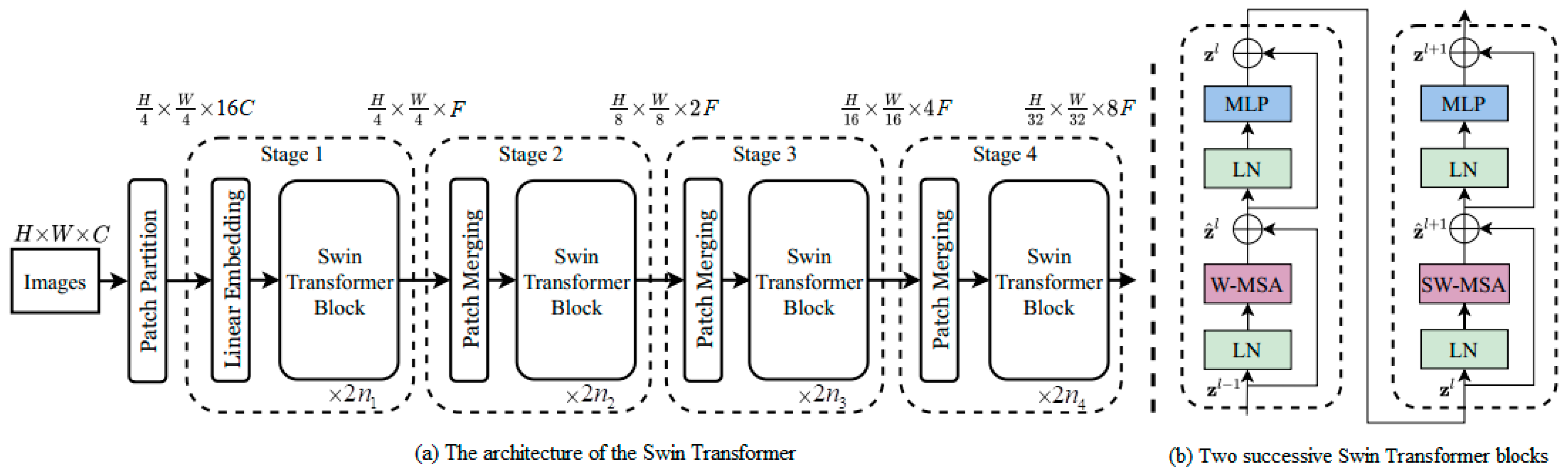
2.2. Swin Transformer

The structure of the Swin Transformer [36] is shown in Figure 2. The size of the original images at the input is $H\times W\times C$, where $H$ is the height of the input image, $W$ is the width of the input image, and $C$ is the number of channels of the input image. For an original image, the Patch partition module splits it into $4\times 4$-sized patches, which are flattened and superimposed to obtain a feature map with the size of ${\displaystyle \frac{H}{4}}\times {\displaystyle \frac{W}{4}}\times 16C$. In “Stage 1”, a Linear Embedding layer is applied on the feature map just obtained to project it to a feature map with dimensions of ${\displaystyle \frac{H}{4}}\times {\displaystyle \frac{W}{4}}\times F$ ($F$ is an arbitrary dimension), and it is then fed into the Swin Transformer block module for processing, where the Swin Transformer block module can be repeated $n_1$ times, each time with two consecutive Swin Transformer blocks, whose structure is shown in Figure 2b. In “Stage 2”, the feature image size obtained after the Patch Merging layer is ${\displaystyle \frac{H}{8}}\times {\displaystyle \frac{W}{8}}\times 2F$, which is fed into the Swin Transformer block module for processing, and here the Swin Transformer block module can be repeated $n_2$ times, each time with two consecutive Swin Transformer blocks, whose structure is shown in Figure 2b. Similarly to the process of “Stage 2”, the sizes of the feature images obtained after “Stage 3” and “Stage 4” are ${\displaystyle \frac{H}{16}}\times {\displaystyle \frac{W}{16}}\times 4F$ and ${\displaystyle \frac{H}{32}}\times {\displaystyle \frac{W}{32}}\times 8F$, respectively. The $n_1,n_2,n_3,{\mathrm{a}\mathrm{n}\mathrm{d} n}_4$ in the Swin Transformer model are configurable integers, such as 1, 1, 3, and 1 in the tiny version (Swin-T) in [36].

The Swin Transformer introduces a novel architecture that diverges from the traditional vision transformer (ViT) by incorporating hierarchical feature maps and a shifted window-based attention mechanism. At its core, the Swin Transformer processes images by dividing them into non-overlapping patches, which are then linearly embedded to form the initial tokens. These tokens are passed through a series of Swin Transformer blocks, each comprising multi-head self-attention (MSA) and a two-layer feed-forward network (FFN) with GELU nonlinearity. The key innovation lies in the shifted window approach to MSA, where the image is partitioned into local windows, and attention is computed within these windows to reduce computational complexity. The window configuration is shifted in subsequent layers to facilitate cross-window connections and capture global context. This hierarchical and local-to-global attention mechanism is central to the Swin Transformer’s design.

3. Swin Transformer-Based Sub-Pixel Displacement Measurement Method

As shown in Figure 3, the proposed ST-SDM obtains sub-pixel displacement values by means of a three-level classification structure, where each level of classification is performed by a separate Swin Transformer structure [36]. The first level of classification, F-ST, is used to calculate sub-pixel displacement values at the “0.1 pixels” pixel level; the second level of classification, S-ST, is used to calculate sub-pixel displacement values at the “0.01 pixels” pixel level; and the third level of classification, T-ST, is used to calculate sub-pixel displacement values at the “0.001 pixels” pixel level.

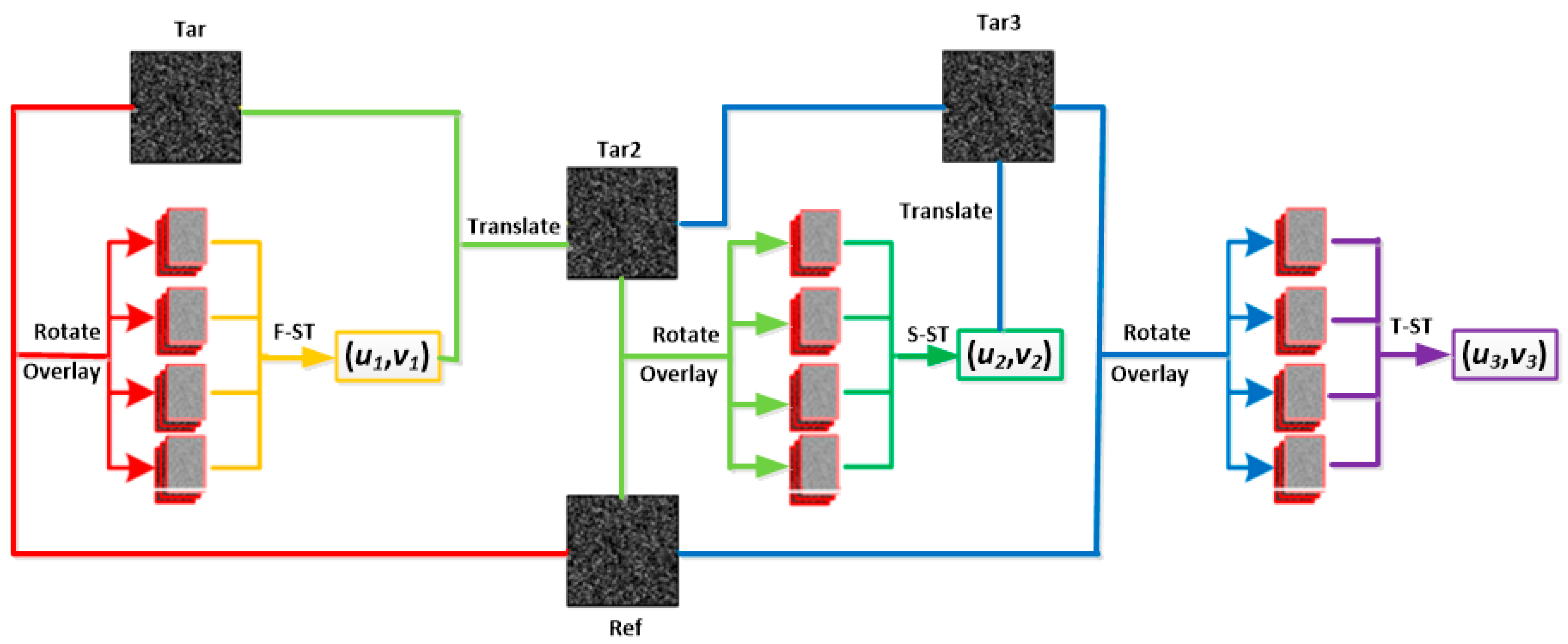
3.1. Three-Level Classification Method for Calculating Sub-Pixel Displacement

For a positive sub-pixel displacement $\mathrm{X}$ belonging to the range of [0, 0.999], it can be decomposed into the form shown in Equation (1):

$$X=\alpha \times 0.1+\beta \times 0.01+\gamma \times 0.001$$

(1)

where $\mathsf{\alpha },\mathsf{\beta },\mathrm{a}\mathrm{n}\mathrm{d} \mathsf{\gamma }$ are integers between 0 and 9, respectively. The tasks of the three-level classification structure of F-ST, S-ST, and T-ST of the ST-SDM are to obtain the three coefficients $\mathsf{\alpha },\mathsf{\beta },\mathrm{a}\mathrm{n}\mathrm{d} \mathsf{\gamma }$ using the Swin Transformer structure, respectively. Thus, there will be 10 categories at each level of classification, which are 0, 1, 2,…, and 9. Specifically, in the first level classification task, F-ST, the coefficient α will be obtained, and the value of α is an integer between 0 and 9, which represents 10 classifications, each of which represents a sub-pixel displacement value within [0, 0.9], i.e., class 0 represents 0 pixels, class 1 represents 0.1 pixels, class 2 represents 0.2 pixels, and so on, and class 9 represents 0.9 pixels. In the second level classification task, S-ST, the coefficient β will be obtained, and the value of β is an integer between 0 and 9, indicating 10 categories, each representing a sub-pixel displacement value within [0, 0.09], i.e., class 0 represents 0 pixels, class 1 represents 0.01 pixels, class 2 represents 0.02 pixels, and so on, and class 9 represents 0.09 pixels. In the third level classification task, T-ST, the coefficient γ will be obtained, and the value of γ is an integer between 0 and 9, indicating 10 categories, each representing a sub-pixel displacement value within [0, 0.009], i.e., class 0 represents 0 pixels, class 1 represents 0.001 pixels, class 2 represents 0.002 pixels, and so on, and class 9 represents 0.009 pixels.

Equation (1) is optimally designed for hierarchical sub-pixel displacement estimation. By aligning with the decimal system, it ensures unique and complete coverage of the range [0, 0.999] through three progressive stages: coarse (α, tenths), medium (β, hundredths), and fine (γ, thousandths) adjustments. This structure inherently supports precision hierarchy, where each Swin Transformer-based classification level (F-ST, S-ST, T-ST) independently resolves displacements at distinct orders of magnitude, avoiding scale overlap or ambiguity. The use of 10 integer classes (0–9) per level guarantees computational tractability, mirroring digit-classification frameworks while maintaining a deterministic one-to-one mapping between displacement values and coefficients. Compared to irregular decompositions (e.g., 0.05/0.005 intervals), and this approach eliminates redundancy, ensures full-range coverage, and aligns seamlessly with the hierarchical feature extraction capabilities of Swin Transformers, enhancing both training stability and interpretability.

In this way, for a sub-pixel displacement value of 0.106 pixels, the classification label obtained from F-ST, S-ST, and T-ST should be “1”, “0”, and “6”, respectively. For a negative sub-pixel displacement, each level of classification will directly output the category “0”. However, this displacement value can still be obtained by the approach described in the next subsection. The advantage of using a three-level categorization task is that although there are only 10 categories at each level of categorization, 1000 categories can actually be obtained.

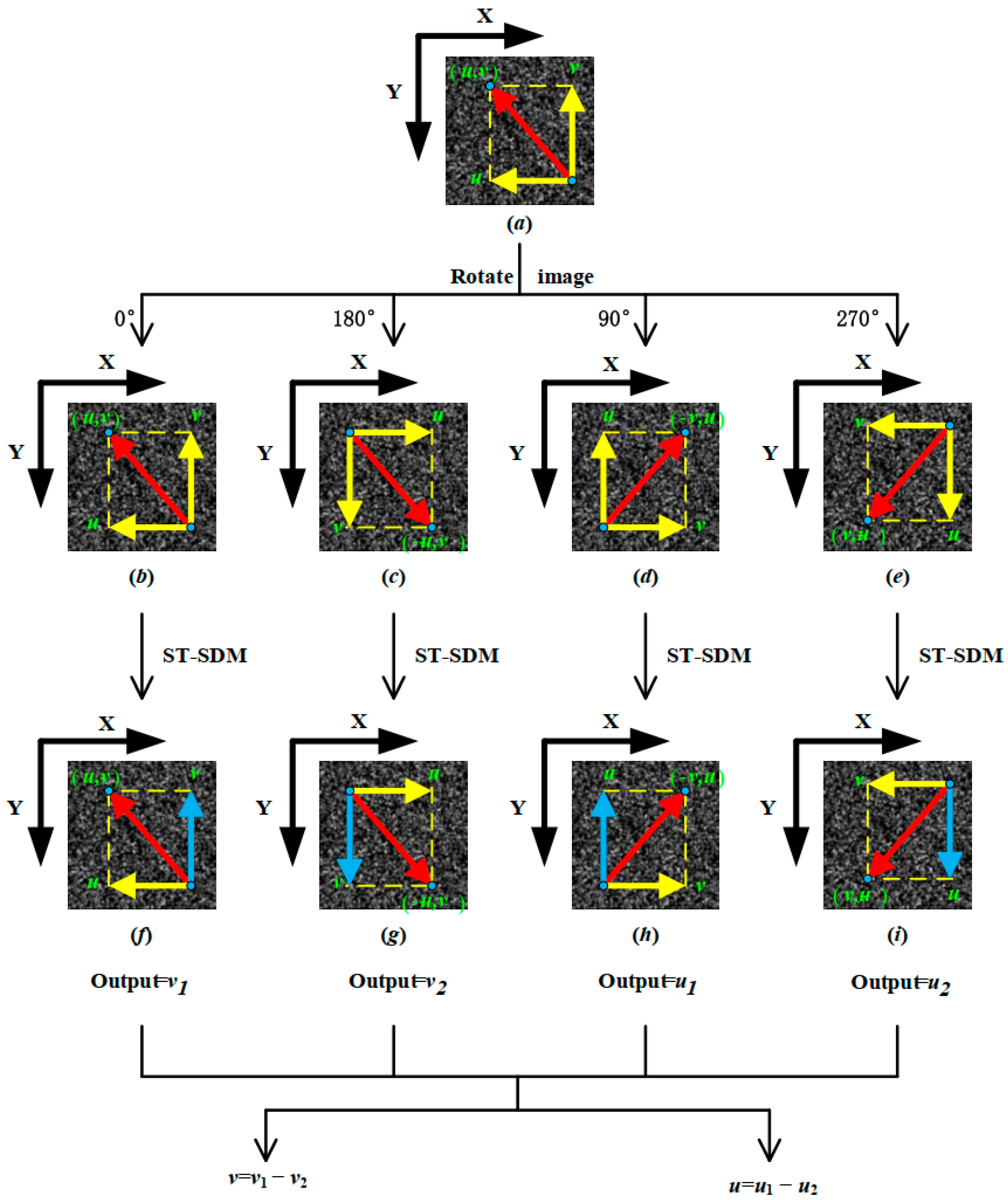
3.2. Rotation-Relative Labeled Value Method

The input of the ST-SDM is images with three channels. For each input image, it is generated by overlapping three single-channel grayscale images, which are the reference image, the target image, and the grayscale image generated by the difference between the grayscale values on the corresponding points of the target image and the reference image.

We define the horizontal rightward and vertical downward sub-pixel displacement values as positive sub-pixel displacement values, which is consistent with the algorithm ST-SDM outputting a nonnegative number of classification labels at each level of classification. However, the displacements can also be negative; thus, at each level of classification, a method called the rotation-relative labeled value method is used to determine the sub-pixel displacement value for that level; and finally, the displacements are integrated to obtain the final sub-pixel displacement value.

The process of the rotation-relative labeled method is shown in Figure 4. For any level of classification of the ST-SDM, for an input image, rotating it clockwise by 0°, 180°, 90°, and 270° will result in four new images, as shown in Figure 4b, Figure 4c, Figure 4d, and Figure 4e, respectively. The images in Figure 4b, Figure 4c, Figure 4d, and Figure 4e are inputted into the classifier of this level of the ST-SDM, assuming that the output categorization labels are ${\mathrm{v}}_1,{\mathrm{v}}_2,{\mathrm{u}}_1,\mathrm{a}\mathrm{n}\mathrm{d} {\mathrm{u}}_2$, respectively, and it can be concluded that the value of the sub-pixel displacement of this input image is (${\mathrm{u}}_1-{\mathrm{u}}_2,{\mathrm{v}}_1-{\mathrm{v}}_2)$. Taking the horizontal component of sub-pixel displacement as an example, since the classifier of the ST-SDM categorizes a negative displacement as category “0”, when the sub-pixel displacement value in the input image is negative, the classification labels ${\mathrm{u}}_1,{\mathrm{v}}_1$ are both “0”, and thus the horizontal component of sub-pixel displacement output at this time is ${-\mathrm{u}}_2$, i.e., a negative value. Similarly, when the sub-pixel displacement value in the input image is positive, the classification labels ${\mathrm{u}}_2,{\mathrm{v}}_2$ are both “0”, and thus the horizontal component of the output sub-pixel displacement value at this time is ${\mathrm{u}}_1$, i.e., a positive value. Thus, the rotation-relative labeled value method solves the problem of positive and negative sub-pixel displacement.

3.3. The Process of the ST-SDM

As shown in Figure 3, the processing of the ST-SDM can be divided into seven steps as follows:

Step 1: The target image, Tar, is rotated clockwise by four angles (0°, 180°, 90°, and 270°) to obtain four new target images, which are overlapped with the reference image, Ref, to obtain four 3-channel images, Img1(1), Img2(1), Img3(1), and Img4(1), respectively.

Step 2: Taking images Img1(1), Img2(1), Img3(1), and Img4(1) as input images, calculate the sub-pixel displacement values at the “0.1 pixels” level using the first level classifier, F-ST, of the ST-SDM, and obtain the sub-pixel displacement values $(u_1,v_1)$.

Step 3: The new target image, Tar2, is obtained after applying translation displacement $(-u_1,-v_1)$ to the target image Tar, and the reference image, Ref, and the four images obtained after rotating Tar2 by four clockwise rotations (0°, 180°, 90°, and 270°) are overlapped, respectively, to obtain four 3-channel images, Img1(2), Img2(2), Img3(2), and Img4(2).

Step 4: Taking images Img1(2), Img2(2), Img3(2), and Img4(2) as input images, calculate the sub-pixel displacement values at the “0.01 pixels” level using the second level classifier, S-ST, of the ST-SDM, and obtain the sub-pixel displacement values $\left(u_2,v_2\right)$.

Step 5: The new target image, Tar3, is obtained after applying translation displacement $(-u_2,{-v}_2)$ to the target image Tar2, and the reference image, Ref, and the four images obtained after rotating Tar3 by four clockwise rotations (0°, 180°, 90°, and 270°) are overlapped, respectively, to obtain four 3-channel images, Img1(3), Img2(3), Img3(3), and Img4(3).

Step 6: Taking images Img1(3), Img2(3), Img3(3), and Img4(3) as input images, calculate the sub-pixel displacement values at the “0.001 pixels” level using the third level classifier, T-ST, of the ST-SDM, and obtain the sub-pixel displacement values $\left(u_3,v_3\right)$.

Step 7: Obtain the final sub-pixel displacement values $\left(u,v\right)=\left(u_1+u_2+u_3,v_1+v_2+v_3\right)$.

4. Experiments and Discussions

In this section, both simulated speckle images experiments and real rigid body translation experiments were performed to verify the performance of the proposed ST-SDM and compared it with the CNN-SDM proposed by Ma [29]. All experiments were performed on a workstation equipped with RAM and 6 GB of NVIDIA GPU (Santa Clara, CA, USA).

4.1. Evaluation Metrics

In this paper, the algorithms are evaluated in terms of computational accuracy and efficiency.

For each actual preset sub-pixel displacement $u_d^j$, the absolute value of the mean displacement error (AVME) $u_e^j$ is defined as Equation (2).

$$u_e^j={\displaystyle \frac{1}{n}}\sum _{i=1}^n\left(|u_i^j-u_d^j|\right)$$

(2)

where n represents the number of all points of interest (POIs, the central points of the subsets), $u_i^j$ represents the calculated displacement value at the $i$-th POI. The relative error in the u direction $R^j$ is defined as Equation (3).

$$R^j={\displaystyle \frac{u_e^j}{u_d^j}}\times 100\%$$

(3)

For $m$ preset sub-pixel displacement $u_d^j(j=\mathrm{1,2},\dots ,m)$, the mean error and the root mean square error (RMSE) of the AVMEs corresponding to them are defined as Equations (4) and (5), respectively.

$$\overline{u}={\displaystyle \frac{1}{m}}\sum _{j=1}^m{u}_e^j$$

(4)

$$RMSE=\sqrt{{\displaystyle \frac{1}{m-1}}\sum _{j=1}^m{\left(u_e^j-\overline{u}\right)}^2}$$

(5)

The absolute values of the mean displacement error (AVME), the relative error, and the root mean square error (RMSE) of the AVMEs are used to verify the computational accuracy of the algorithms. Computational efficiency is quantified as the average time taken by the algorithms to process each image.

4.2. Simulated Speckle Image Experiments

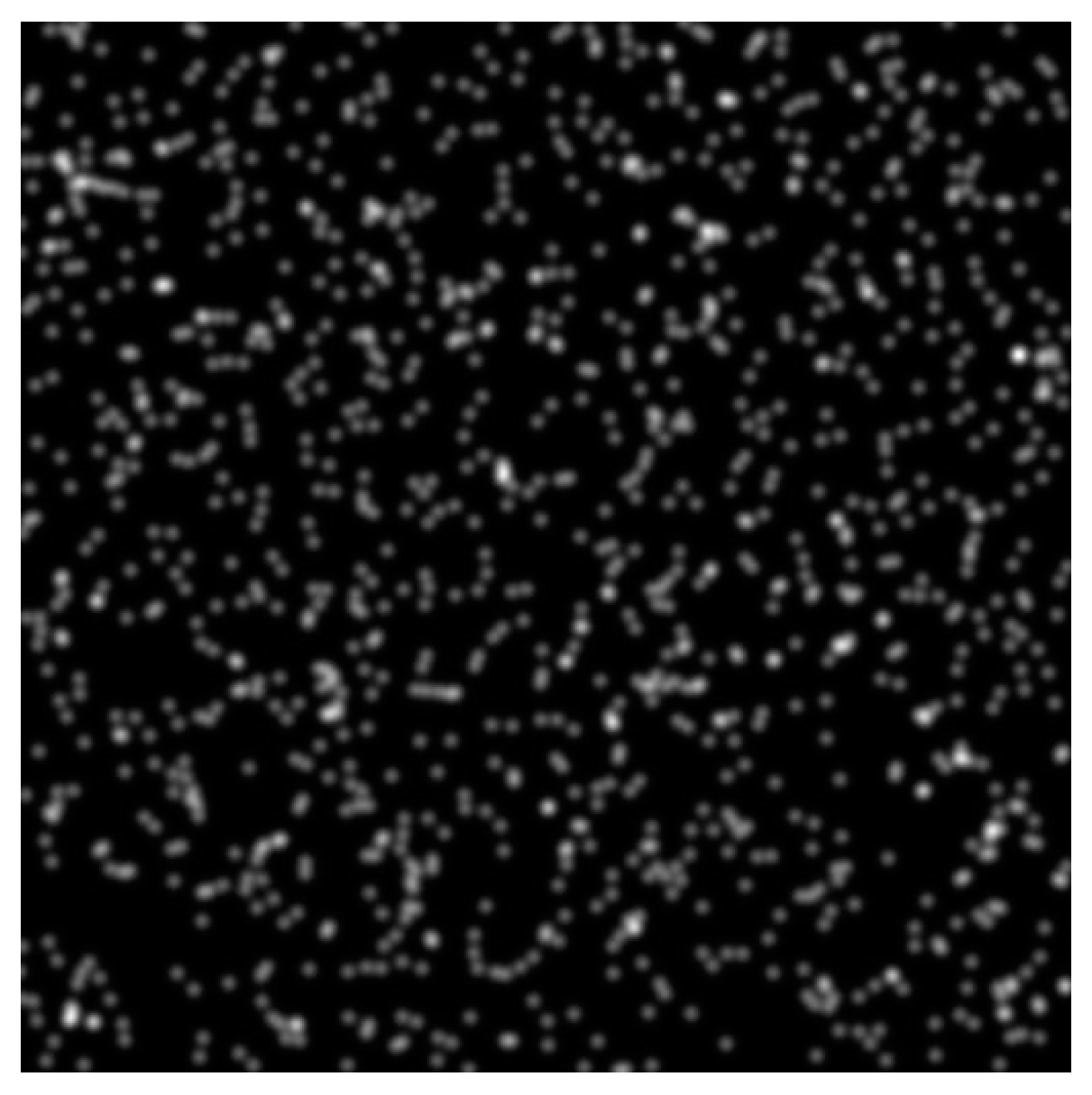
4.2.1. Simulated Speckle Image Generation

A computerized method for generating speckle images [16,17] is used to randomly generate the simulated speckle images. The simulated speckle function is defined as follows:

$$\left\{\begin{array}{c}{I}_1\left(x,y\right)={\displaystyle \sum _{k=1}^n}{I_{0}e}^{-{\displaystyle \frac{{\left(x-x_k\right)}^2+{\left(y-y_k\right)}^2}{R^2}}}\\ I_2\left(x,y\right)={\displaystyle \sum _{k=1}^n}{I_{0}e}^{-{\displaystyle \frac{{\left(x-{x_k}^{\prime }\right)}^2+{\left(y-{y_k}^{\prime }\right)}^2}{R^2}}}\end{array}\right.$$

(6)

where $I_1\left(x,y\right)$ and $I_2\left(x,y\right)$ represent the gray scale of the speckle images generated before and after the deformation, respectively. $I_0$ is the light intensity at the center of the speckle, $n$ is the number of speckles, and $R$ is the radius of the speckle. $\left(x_k,y_k\right)$ and $\left({x_k}^{\prime },{y_k}^{\prime }\right)$ are the spot center position of the speckle pattern before and after the deformation, respectively.

The stretching, compressing, translating, and rotating of a speckle image can be simulated using the following equation:

$$\left\{\begin{array}{c}{x_k}^{\prime }=x_k+u_0+x_k{u}_x+y_k{u}_y\\ {y_k}^{\prime }=y_k+v_0+x_k{v}_x+y_k{v}_y\end{array}\right.$$

(7)

where $u_0$, $v_0$ is the displacement along the x and y direction; $u_x$, $u_y$ are the displacement gradients in the $x$ direction, $v_x$, $v_y$ are displacement gradients in the$y$ direction.

The simulated speckle images were generated with $I_0$ = 80, $n$ = 2000, ROI = 512 pixels × 512 pixels, $R$ = 2 pixels, and a sample which is shown in Figure 5.

The dataset generation methods are as follows:

(1)

Translation Dataset Generation Method: First, speckle images are generated using the method described earlier, and one of them is randomly selected as the reference image. Next, the selected speckle image is translated to the right along the horizontal direction $x$ in steps of 0.01 pixels for a total of 100 steps, generating 100 target images. Finally, using the square dataset expansion method described in Section 4.3.1, the translation dataset is expanded, resulting in a total of 80,200 speckle images.

(2)

Stretching Dataset Generation Method: First, speckle images are generated using the method described earlier, and 50 of them are randomly selected as reference images. Next, the selected speckle images are stretched in the horizontal direction $x$ with $u_x=0.001$ and $u_y=0.01$ using Equation (7), and the stretched speckle images are used as target images. Finally, using the square dataset expansion method described in Section 4.3.1, the stretching dataset is expanded, resulting in a total of 20,100 speckle images.

(3)

Experimental Dataset Composition: The datasets obtained from the above two steps are combined to form the complete experimental dataset. Of the sample data, 80% are used for training, and the remaining 20% are used for testing.

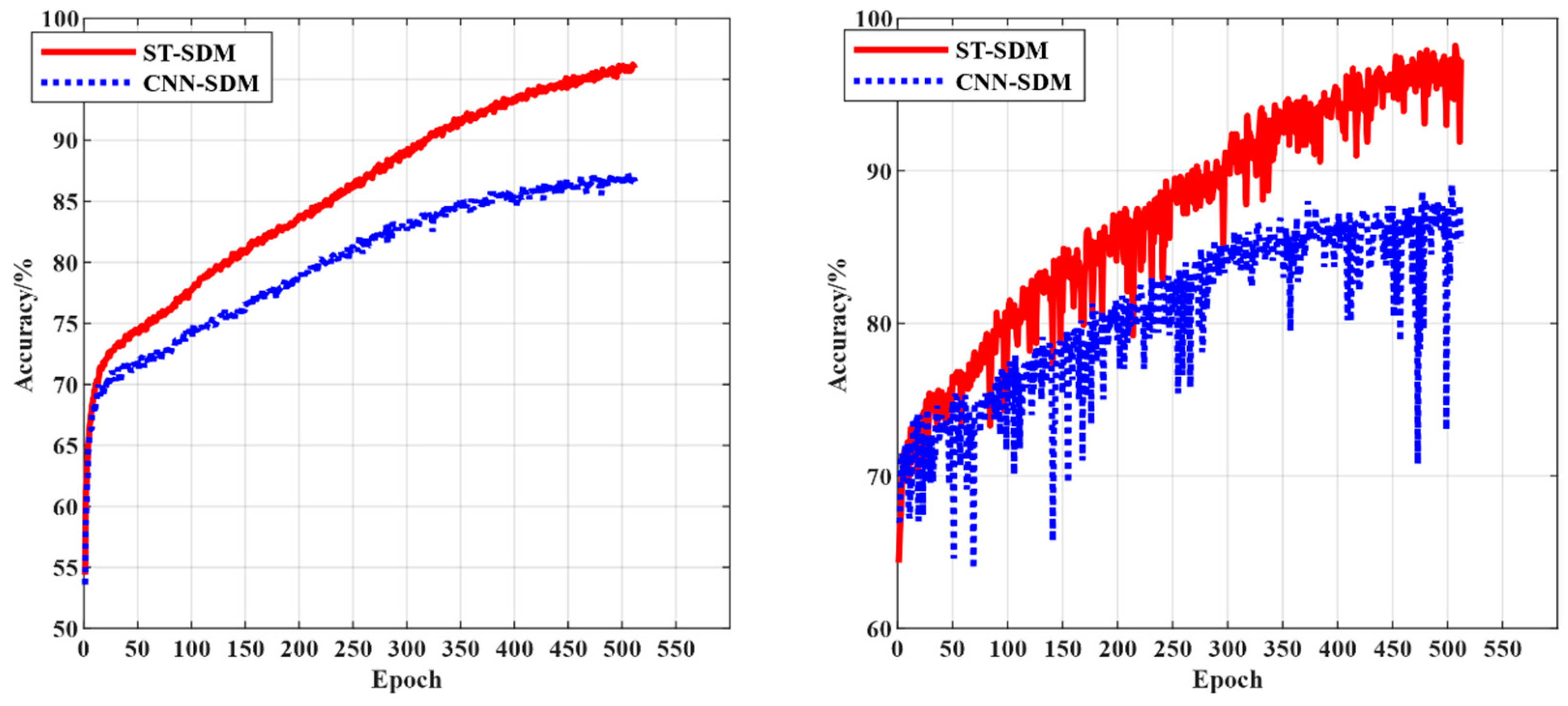
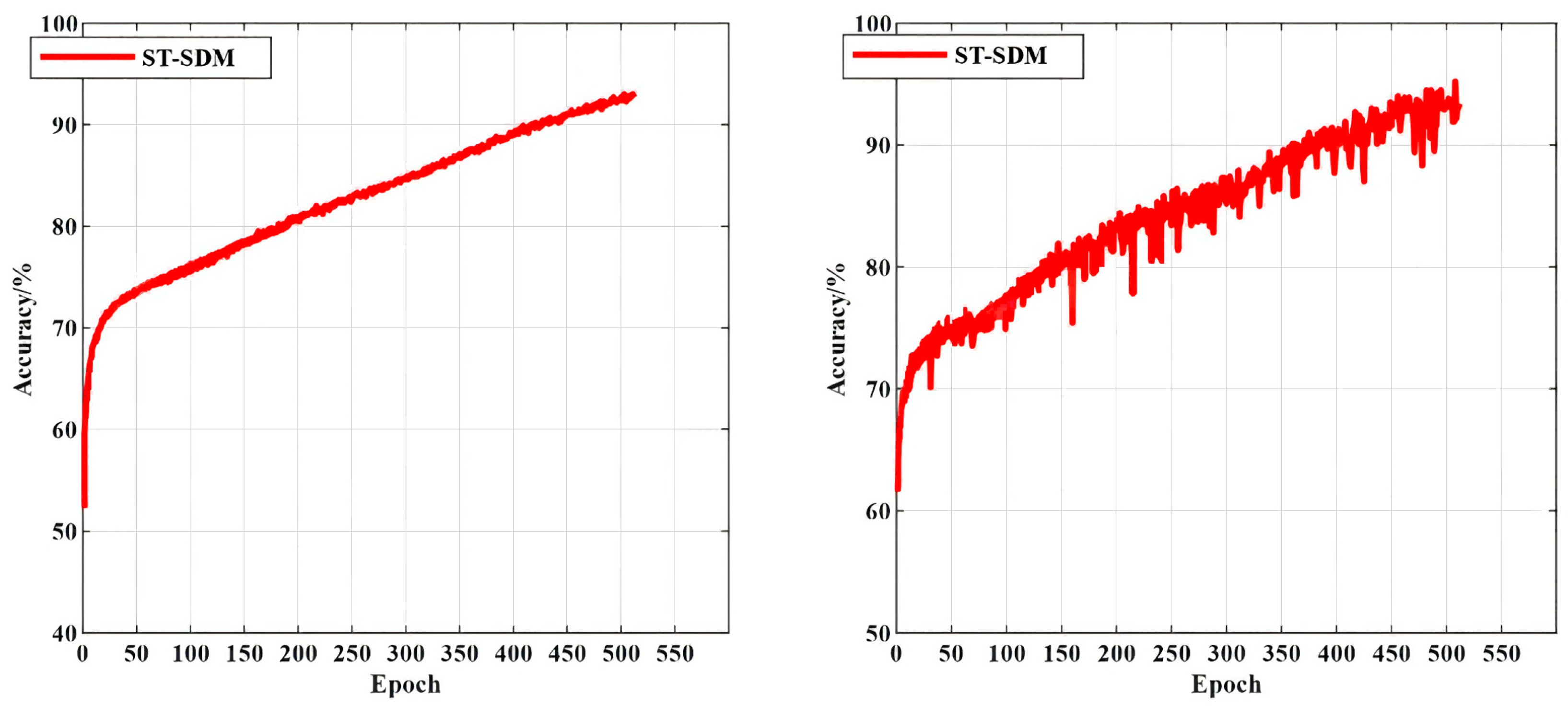
4.2.2. Comparative Analysis of Model Accuracy

Since the CNN-SDM [29] has only two levels of classification while the ST-SDM has three levels of classification, model accuracy comparisons can only be made on the first two levels of classification. The variation in accuracy with the number of training steps (Epochs) for the first and second level classification of the two models, the ST-SDM and the CNN-SDM, are shown in Figure 6 and Figure 7, respectively, and the variation in accuracy with the number of training steps for the third level classification of the ST-SDM model is shown in Figure 8, where the left part of each figure shows the trend of the models’ accuracy on the training dataset with the number of training steps, and the right part shows the trend of the models’ accuracy on the test dataset with the number of training steps.

As can be seen from Figure 6, Figure 7 and Figure 8, the accuracy curve of the ST-SDM on the training dataset is relatively smooth, and the accuracy curve on the test dataset fluctuates more, but, in general, they are not very different. Meanwhile, the accuracy of the first level of classification is better than that of the second level of classification, and the accuracy of the second level of classification is better than that of the third level of classification. From Figure 6 and Figure 7, it can be seen that the accuracy of the first two levels of classification of the ST-SDM is higher than the accuracy of the corresponding level of classification of the CNN-SDM. Therefore, the ST-SDM proposed in this paper outperforms the CNN-SDM in terms of accuracy.

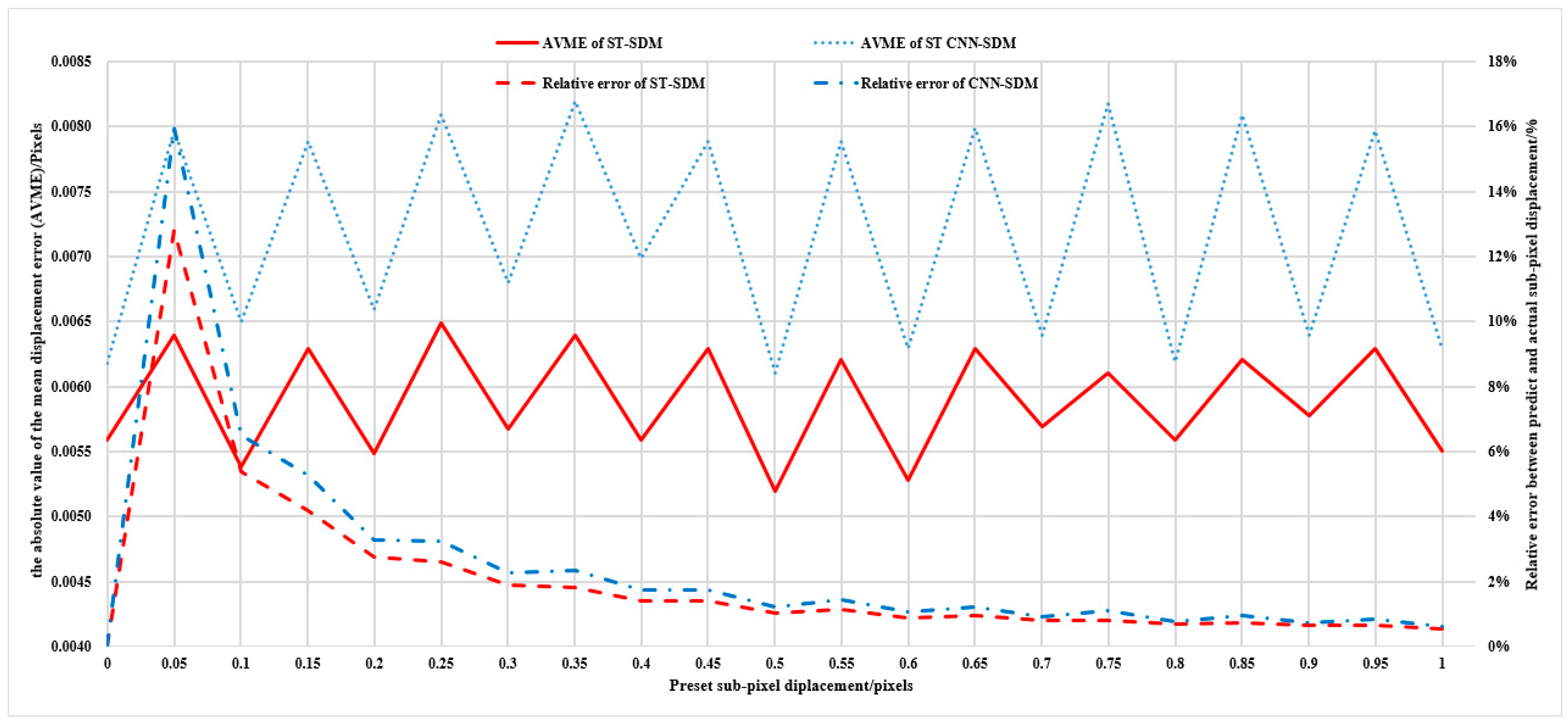
4.2.3. Comparative Analysis of Model Calculation Accuracy

A number of test samples are selected, and the preset true displacement values in the horizontal u direction are from 0 pixels to 1 pixel, with an increment of 0.05 pixels, which are predicted by the ST-SDM model and the CNN-SDM model, respectively, and the absolute values of the mean displacement errors (AVMEs) and relative errors between the predicted values and the true values are shown in Figure 9. As shown in Figure 9, the AVMEs for the ST-SDM are from 5.2 × 10⁻³ to 6.5 × 10⁻³ pixels, with the mean error and the RMSE of the AVMEs are 5.89 × 10⁻³ and 0.42 × 10⁻³ pixels, respectively. The AVMEs for the CNN-SDM are from 6.1 × 10⁻³ to 8.2 × 10⁻³ pixels, with the mean error and the RMSE of the AVMEs being 7.18 × 10⁻³ and 0.84 × 10⁻³ pixels, respectively. Accordingly, the relative errors of the ST-SDM range from 0.55% to 12.79%, while the relative errors of the CNN-SDM range from 0.63% to 15.94%. The maximum and minimum values of the AVMEs and the RMSEs of two deep learning-based algorithms (the CNN-SDM and the ST-SDM) as well as several traditional algorithms (SF, GC, FANR) from the literature [16] are shown in

Table 1. Comparison of the AVMEs and the RMSEs of the seven algorithms.

Algorithm	AVME (×10−3 Pixels)		RMSE (×10−3 Pixels)
	Minimum	Maximum
SF	13.80	24.9	16.00
GC	6.00	13.5	8.00
FANR	1.00	4.31	1.00
IC-GN	0.90	4.24	0.97
IV-ICGN	0.31	3.56	0.90
CNN-SDM	6.10	8.20	0.84
ST-SDM	5.20	6.50	0.42

. As shown in Table 1, the accuracy of the two deep learning-based algorithms, the CNN-SDM and the ST-SDM, outperforms that of the traditional algorithms SF and GC. However, their accuracy is lower than that of the traditional algorithms FANR, IC-GN, and IV-ICGN. Additionally, the ST-SDM demonstrates higher accuracy than the CNN-SDM.

4.2.4. Comparative Analysis of Model Computational Efficiency

The average processing time per image for both the CNN-SDM and the ST-SDM models on this experimental dataset is listed in

Table 2. Comparison of computing time between two algorithms.

Sub-Pixel Displacement Measurement Method	ST-SDM	CNN-SDM
Average time spent per image (S)	0.106	0.368

, and the average processing time per image for the ST-SDM is smaller than that for the CNN-SDM. Therefore, the algorithm of the ST-SDM is more efficient.

4.3. Real Rigid Body Translation Experiments

4.3.1. Square Dataset Expansion Method

To meet deep learning algorithms’ requirement of a large amount of training data to demonstrate their excellent performance, a method for quickly expanding the dataset in the case of a limited dataset, the Square Dataset Expansion Method, is proposed in this section.

For an image $p$, firstly, $p$ is translated horizontally by $i(i=\mathrm{0,1},2,\dots ,m)$ steps and vertically by $j(j=\mathrm{0,1},2,\dots ,n)$ steps to obtain a new image $q_{ij}(i=\mathrm{0,1},2,\dots m,j=\mathrm{0,1},2,\dots ,n)$, then we will obtain a total of $t=(m+1)(n+1)$ images. Secondly, $q_{ij}(i=\mathrm{0,1},2,\dots m,j=\mathrm{0,1},2,\dots ,n)$ is rotated clockwise by 0°, 180°, 90°, and 270°, then $4t$ images will be produced. Finally, take any two of these images as the reference image and the target image, respectively, and generate an input image with labels into the dataset by the method described in the previous section, and a total of $T(m,n)$ (as shown in the following Equation (8)) input images will be generated.

$$T\left(m,n\right)={\displaystyle \frac{\left(4t+1\right)\times 4t}{2}}={8\left(m+1\right)}^2{\left(n+1\right)}^2+2\left(m+1\right)\left(n+1\right)$$

(8)

Taking m = n = 10 as an example, when the image $p$ is translated horizontally and vertically by 0, 1, 2, 3,…, and 10 steps, respectively, we obtain 11 × 11 = 121 images, and the collection of these images is denoted as set $S1$. Subsequently, by rotating each image in $S1$ clockwise by 0°, 180°, 90°, and 270°, we generate 4 × 121 new images, and the set comprising these new images is denoted as $S2$. From $S2$, we select any two images, one to serve as the reference image and the other as the target image. Using the method described in Section 3.2, we generate an input image from each pair and add it to the training set $S$. Ultimately, the training set $S$ contains (4 × 121 + 1) × (4 × 121)/2= 117,370 images.

4.3.2. Experimental Composition and Experimental Procedure

The composition of the experimental system is the same as that in [16], as shown in Figure 10, where ➀ is the glass with speckles, ➁ is the light source equipment, which has a maximum light intensity of 5600 lm, ➂ is an electronically controlled translation stage that boasts a positioning accuracy of ±5 µm and a repeatability of ±2 µm, capable of applying precise displacements in both the $X$ and $Y$ directions, and ➃ is the CCD camera.

The experimental process is as follows:

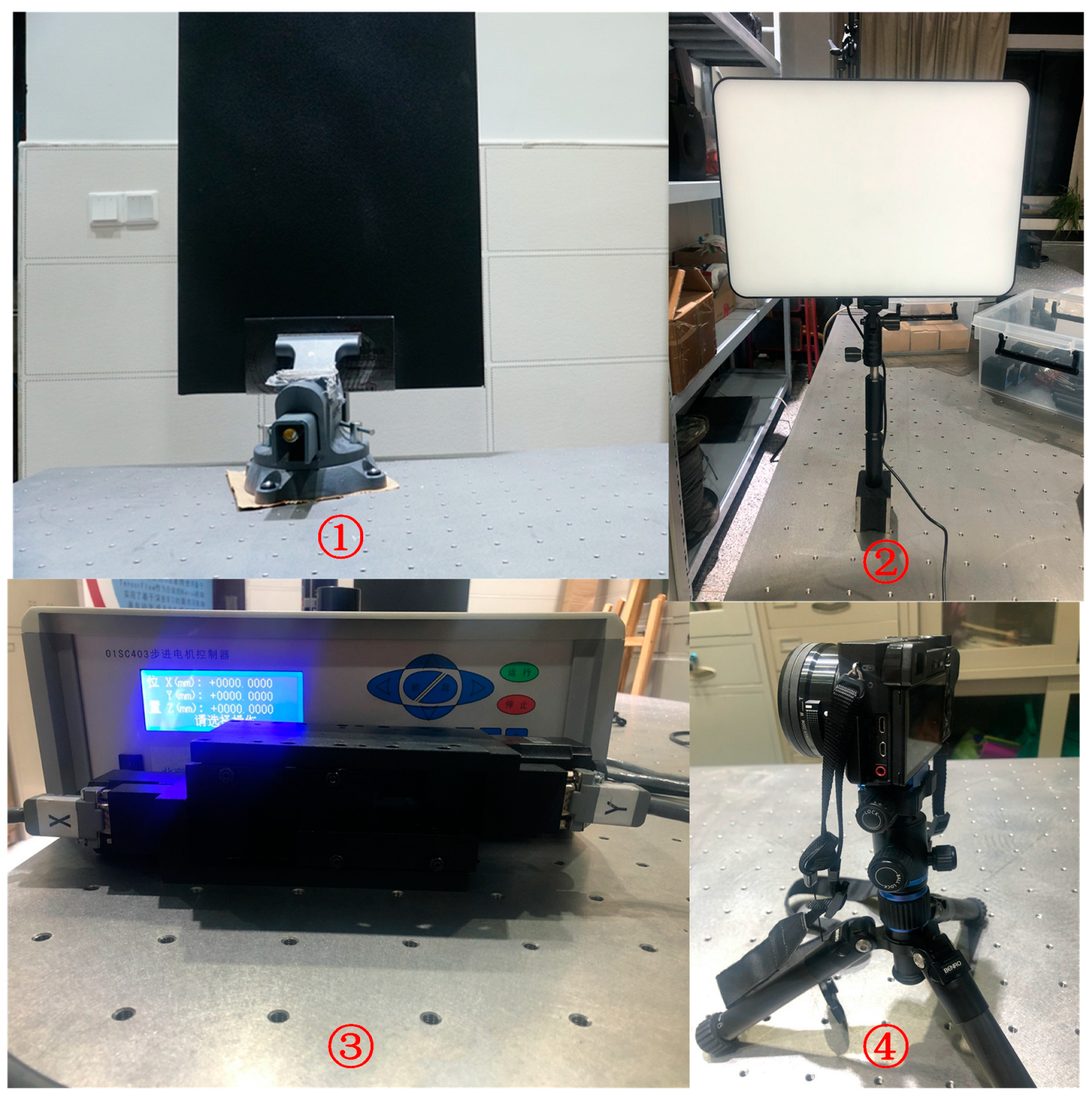
• We made speckles on the glasses. While keeping the spray gun at a constant distance from the glass and perpendicular to it, the matte black paint was uniformly sprayed on the surface of the cleaned glasses to form randomly distributed and uniformly sized speckles on it.
• We prepared the experimental setup. Firstly, the glasses with speckles were fixed on the holder, then the electronically controlled translation stage and the light source equipment were fixed on the optical platform, and finally the CCD camera was fixed on the electronically controlled translation stage.
• We determined the pixel equivalent of the camera system, which is 0.400 mm/pixel in this experiment.
• We obtained the speckle image before displacement. Without applying any displacement, the first speckle images of sizes of 512 pixels ×512 pixels were obtained with the CCD camera, as shown in Figure 11.
• We obtained the speckle image after displacement. Displacement in the $X$ direction was applied to the electronically controlled translation stage for 10 steps of 0.1 mm each, and 10 scatter plots were obtained with the CCD camera, each of which had a size of 512 pixels ×512 pixels.
• We conducted the segmentation of speckle images. In order to generate enough training samples, the speckle image before displacement and the speckle image after displacement were divided. The segmentation method is as follows: for each speckle image, with a spacing of 30 pixels in the $X, Y$ direction, take an image of a size of 64 pixels × 64 pixels as a sub speckle image, and 15 × 15 = 225 sub speckle images can be obtained. The sub speckle images obtained from the speckle image before displacement were used as the reference images, and the sub speckle images obtained from the speckle image after displacement were used as the target images.
• We generated the dataset. The images obtained in the previous step were expanded using the square dataset expansion method proposed in the previous section, and finally $225\times T\left(\mathrm{10,0}\right)=\mathrm{222,750}$ sample data were obtained. We used 80% of the sample data for training and the remaining 20% for testing.
• We conducted a comparison experiment. The ST-SDM model and the CNN-SDM model were trained and tested, respectively, and the experiment results are shown in Figure 12.

4.3.3. Comparative Experimental Analysis

As shown in Figure 12, in terms of the overall trend of the two curves, it can be seen that the absolute values of the mean displacement error (AVME) of the ST-SDM algorithm are smaller than those of the CNN-SDM algorithm. The former are basically between 0.011 pixels and 0.015 pixels with the mean error and the RMSE of the AVMEs being 0.0126 and 0.00089 pixels, respectively, while the latter are between 0.013 pixels and 0.017 pixels with the mean error and the RMSE of the AVMEs being 0.0150 and 0.00090 pixels, respectively. Accordingly, the relative errors of the ST-SDM range from 1.48% to 11.94%, while the relative errors of the CNN-SDM range from 1.65% to 14.56%. From this, it can be concluded that the ST-SDM algorithm has good accuracy and robustness in real environment measurements.

4.4. Discussion

Based on the precision comparison of various algorithms in Section 4.2.3, the two deep learning-based algorithms (the ST-SDM and the CNN-SDM) exhibit higher AVMEs but significantly lower RMSEs compared to traditional algorithms. This indicates that deep learning algorithms possess superior stability over traditional methods. Future work will focus on designing more accurate deep learning algorithms to address the sub-pixel displacement measurement problem more effectively. Additionally, the ST-SDM demonstrates higher computational accuracy than the CNN-SDM. The primary reason is that the CNN-SDM employs the traditional Convolutional Neural Network (CNN) approach, whereas our ST-SDM utilizes the Swin Transformer. The Swin Transformer, with its unique hierarchical architecture and shifted window mechanism, is more efficient in capturing local features and global context information when handling image classification tasks, thereby achieving higher performance compared to traditional CNN methods.

According to the comparison experiments in Section 4.2.4, the ST-SDM has higher computational efficiency than the CNN-SDM. This is made available thanks to the fact that we employ a Swin Transformer structure in each level of classification, which we briefly describe in Section 2.2. The comparison of a Swin Transformer structure with a ViT and a CNN in terms of computational speed and computational storage requirements has been discussed in detail in the literature [36,37].

The square dataset expansion method provides a universal and effective solution for expanding speckle pattern training datasets, especially when the number of training samples is extremely limited. This method can significantly enhance the scale and diversity of the dataset, thereby creating more favorable conditions for model training. However, this augmentation approach may also have certain limitations. Specifically, the network model trained using this method may lack sufficient generalization ability. Although the model’s performance on the training dataset has been verified to be satisfactory through previous experiments, its performance on entirely new, unseen data may not be guaranteed, which could affect the practical application value of the model.

Although the ST-SDM algorithm proposed in this paper provides a novel solution for the sub-pixel displacement measurement problem, the current experimental research is not yet comprehensive. For instance, the algorithm’s adaptability under varying lighting conditions and other constraints, as well as its real-time performance, have not been fully evaluated. Future research could integrate adaptive illumination normalization (e.g., Retinex-based preprocessing or deep learning-driven intensity correction) and hybrid architectures that combine lightweight neural networks with physics-based speckle correlation models to balance precision and efficiency. Strategies such as hardware acceleration (FPGA/GPU deployment) and domain-generalizable training with synthetic speckle data augmented with realistic noise and lighting perturbations could enhance robustness.

In addition, while vision transformers (ViTs) have demonstrated remarkable success in diverse computer vision tasks (e.g., classification, detection, and segmentation), their potential to enhance digital speckle correlation methods (DSCMs) remains unexplored—a gap offering significant opportunities to improve deformation analysis in complex environments. However, integrating ViTs into DSCMs faces critical challenges: (1) the computational complexity of global self-attention mechanisms scales quadratically with input resolution, conflicting with real-time processing demands; (2) limited domain-specific data for speckle patterns with structured noise risks overfitting and undermines generalization; (3) ViTs have reduced sensitivity to localized intensity gradients, which are essential for sub-pixel displacement accuracy; and (4) hardware constraints are exacerbated by ViTs’ resource-intensive architecture. Addressing these challenges necessitates hybrid approaches (e.g., ViT-CNN fusion), lightweight attention optimization, and domain-adaptive training to harmonize ViTs’ global contextual strengths with a DSCM’s precision and efficiency requirements.

5. Conclusions

In this paper, a Swin Transformer-based sub-pixel displacement measurement method, a ST-SDM, is proposed to complete the calculation of sub-pixel displacement values through a three-level classification task. The model adopts a three-level classification task, making it easier to obtain the training dataset, the network structure is simple, and there are only 10 categories in each level, so that the sub-pixel displacement values can be classified into 1000 classes by the combination of the three levels of classification, i.e., to obtain sub-pixel displacement values with three decimal places. Firstly, the rotation-relative labeled value method is used to solve the problem of positive and negative displacements, and then a flat dataset expansion method is proposed to rapidly expand the dataset to meet the requirement of deep learning algorithms that need a large amount of training data to show excellent performance, and finally, the accuracy is verified by simulation experiments and the robustness is verified by real experiments.

References

1. Peters, W.H.; Ranson, W.F. Digital Imaging Techniques in Experimental Stress Analysis. Opt. Eng. 1982, 21, 427–431. [Google Scholar] [CrossRef]
2. Chen, D.J.; Chiang, F.P.; Tan, Y.S.; Don, H.S. Digital speckle-displacement measurement using a complex spectrum method. Appl. Opt. 1993, 32, 1839. [Google Scholar] [CrossRef] [PubMed]
3. Schreier, H.W.; Sutton, M.A. Systematic errors in digital image correlation due to undermatched subset shape functions. Exp. Mech. 2002, 42, 303–310. [Google Scholar] [CrossRef]
4. Wang, H.W.; Kang, Y.L. Improved digital speckle correlation method and its application in fracture analysis of metallic foil. Opt. Eng. 2002, 41, 436–445. [Google Scholar] [CrossRef]
5. Tong, X.; Ye, Z.; Xu, Y.; Gao, S.; Xie, H.; Du, Q.; Liu, S.; Xu, X.; Liu, S.; Luan, K.; et al. Image Registration with Fourier-Based Image Correlation: A Comprehensive Review of Developments and Applications. IEEE J. Sel. Top. Appl. Earth Obs. Remote Sens. 2019, 12, 4062–4081. [Google Scholar] [CrossRef]
6. Khoo, S.-W.; Karuppanan, S.; Tan, C.-S. A Review of Surface Deformation and Strain Measurement Using Two-Dimensional Digital Image Correlation. Metrol. Meas. Syst. 2016, 23, 461–480. [Google Scholar] [CrossRef]
7. Su, Y.; Zhang, Q.; Xu, X.; Gao, Z. Quality assessment of speckle patterns for DIC by consideration of both systematic errors and random errors. Opt. Lasers Eng. 2016, 86, 132–142. [Google Scholar] [CrossRef]
8. Bai, P.; Xu, Y.; Zhu, F.; Lei, D. A novel method to compensate systematic errors due to undermatched shape functions in digital image correlation. Opt. Lasers Eng. 2020, 126, 105907. [Google Scholar] [CrossRef]
9. Zhong, F.; Quan, C. Efficient digital image correlation using gradient orientation. Opt. Laser Technol. 2018, 106, 417–426. [Google Scholar] [CrossRef]
10. Wang, L.; Bi, S.; Lu, X.; Gu, Y.; Zhai, C. Deformation measurement of high-speed rotating drone blades based on digital image correlation combined with ring projection transform and orientation codes. Measurement 2019, 148, 106899. [Google Scholar] [CrossRef]
11. Pan, B.; Li, K.; Tong, W. Fast, Robust and Accurate Digital Image Correlation Calculation Without Redundant Computations. Exp. Mech. 2013, 53, 1277–1289. [Google Scholar] [CrossRef]
12. Shao, X.X.; Dai, X.J.; He, X.Y. Noise robustness and parallel computation of the inverse compositional Gauss–Newton algorithm in digital image correlation. Opt. Lasers Eng. 2015, 71, 9–19. [Google Scholar] [CrossRef]
13. Zhang, L.; Wang, T.; Jiang, Z.; Kemao, Q.; Liu, Y.; Liu, Z.; Tang, L.; Dong, S. High accuracy digital image correlation powered by GPU-based parallel computing. Opt. Lasers Eng. 2015, 69, 7–12. [Google Scholar] [CrossRef]
14. Huang, J.; Zhang, L.; Jiang, Z.; Dong, S.; Chen, W.; Liu, Y.; Liu, Z.; Zhou, L.; Tang, L. Heterogeneous parallel computing accelerated iterative subpixel digital image correlation. Sci. China Technol. Sci. 2018, 61, 74–85. [Google Scholar] [CrossRef]
15. Yang, J.; Huang, J.; Jiang, Z.; Dong, S.; Tang, L.; Liu, Y.; Liu, Z.; Zhou, L. SIFT-aided path-independent digital image correlation accelerated by parallel computing. Opt. Lasers Eng. 2020, 127, 105964. [Google Scholar] [CrossRef]
16. Chen, Q.; Tie, Z.; Hong, L.; Qu, Y.; Wang, D. Improved Search Algorithm of Digital Speckle Pattern Based on PSO and IC-GN. Photonics 2022, 9, 167. [Google Scholar] [CrossRef]
17. Zhou, P.; Goodson, K.E. Subpixel displacement and deformation gradient measurement using digital image/speckle correlation. Opt. Eng. 2001, 40, 1613–1620. [Google Scholar] [CrossRef]
18. Zhang, J.; Jin, G.; Ma, S.; Meng, L. Application of an improved subpixel registration algorithm on digital speckle correlation measurement. Opt. Laser Technol. 2003, 35, 533–542. [Google Scholar] [CrossRef]
19. Hung, P.C.; Voloshin, A.S. In-plane strain measurement by digital image correlation. J. Braz. Soc. Mech. Sci. Eng. 2003, 25, 215–223. [Google Scholar] [CrossRef]
20. Zhao, J.; Zhou, Y.; Zhao, J.; Dong, F.; Jiang, X.; Gong, K. Mover Position Detection for PMSLM Based on Line-Scanning Fence Pattern and Subpixel Polynomial Fitting Algorithm. IEEE/ASME Trans. Mechatron. 2020, 25, 44–54. [Google Scholar] [CrossRef]
21. Bruck, H.A.; McNeill, S.R.; Sutton, M.A.; Peters, W.H. Digital Image Correlation Using Newton-Raphson Method of Partial Differential Correction. Exp. Mech. 1989, 29, 261–267. [Google Scholar] [CrossRef]
22. Baker, S.; Matthews, I. Equivalence and efficiency of image alignment algorithms. In Proceedings of the 2001 IEEE Computer Society Conference on Computer Vision and Pattern Recognition CVPR 2001, Kauai, HI, USA, 8–14 December 2001. [Google Scholar] [CrossRef]
23. Sutton, M.A.; Orteu, J.J.; Schreier, H.W. Image Correlation for Shape, Motion and Deformation Measurements: Basic Concepts, Theory and Applications; Springer: New York, NY, USA, 2009; pp. 70–79. [Google Scholar]
24. Pitter, M.; See, C.W.; Somekh, M. Subpixel Microscopic Deformation Analysis Using Correlation and Artificial Neural Networks. Opt. Express 2001, 8, 322–327. [Google Scholar] [CrossRef] [PubMed]
25. Liu, X.; Tan, Q. Subpixel In-Plane Displacement Measurement Using Digital Image Correlation and Artificial Neural Networks. In Proceedings of the 2010 Symposium on Photonics and Optoelectronics SOPO 2010, Chengdu, China, 19–21 June 2010. [Google Scholar] [CrossRef]
26. Min, H.-G.; On, H.-I.; Kang, D.-J.; Park, J.-H. Strain Measurement During Tensile Testing Using Deep Learning-Based Digital Image Correlation. Meas. Sci. Technol. 2020, 31, 015014. [Google Scholar] [CrossRef]
27. Boukhtache, S.; Abdelouahab, K.; Berry, F.; Blaysat, B.; Grédiac, M.; Sur, F. When Deep Learning Meets Digital Image Correlation-ScienceDirect. Opt. Lasers Eng. 2020, 136, 106308. [Google Scholar] [CrossRef]
28. Huang, J.; Sun, C.; Lin, X. Displacement Field Measurement of Speckle Images Using Convolutional Neural Network. Acta Opt. Sin. 2021, 41, 2012002. [Google Scholar] [CrossRef]
29. Ma, C.; Ren, Q.; Zhao, J. Optical-numerical method based on a convolutional neural network for full-field subpixel displacement measurements. Opt. Express 2021, 29, 9137. [Google Scholar] [CrossRef] [PubMed]
30. Li, H.; Weng, J.; Shi, Y.; Gu, W.; Mao, Y.; Wang, Y.; Liu, W.; Zhang, J. An Improved Deep Learning Approach for Detection of Thyroid Papillary Cancer in Ultrasound Images. Sci. Rep. 2018, 8, 6600. [Google Scholar] [CrossRef]
31. Tsagkatakis, G.; Aidini, A.; Fotiadou, K.; Giannopoulos, M.; Pentari, A.; Tsakalides, P. Survey of Deep-Learning Approaches for Remote Sensing Observation Enhancement. Sensors 2019, 19, 3929. [Google Scholar] [CrossRef]
32. Seeja, R.D.; Suresh, A. Deep Learning Based Skin Lesion Segmentation and Classification of Melanoma Using Support Vector Machine (SVM). Asian Pac. J. Cancer Prev. 2019, 20, 1555–1561. [Google Scholar] [CrossRef]
33. Boukhtache, S.; Abdelouahab, K.; Bahou, A.; Berry, F.; Blaysat, B.; Grédiac, M.; Sur, F. A lightweight convolutional neural network as an alternative to DIC to measure in-plane displacement fields. Opt. Lasers Eng. 2023, 167, 107367. [Google Scholar] [CrossRef]
34. Khan, A.; Sohail, A.; Zahoora, U.; Qureshi, A.S. A Survey of the Recent Architectures of Deep Convolutional Neural Networks. Artif. Intell. Rev. 2020, 53, 5455–5516. [Google Scholar] [CrossRef]
35. Kim, J.H.; Heo, B.; Lee, J.S. Joint Global and Local Hierarchical Priors for Learned Image Compression. In Proceedings of the 2022 IEEE/CVF Conference on Computer Vision and Pattern Recognition CVPR 2022, New Orleans, LA, USA, 18–24 June 2022. [Google Scholar] [CrossRef]
36. Liu, Z.; Lin, Y.; Cao, Y.; Hu, H.; Wei, Y.; Zhang, Z.; Lin, S.; Guo, B. Swin Transformer: Hierarchical Vision Transformer using Shifted Windows. In Proceedings of the 2021 IEEE/CVF International Conference on Computer Vision ICCV 2021, Montreal, QC, Canada, 10–17 October 2021. [Google Scholar] [CrossRef]
37. Vaswani, A.; Shazeer, N.; Parmar, N.; Uszkoreit, J.; Jones, L.; Gomez, A.N.; Kaiser, L.; Polosukhin, I. Attention is all you need. arXiv 2017, arXiv:1706.03762. [Google Scholar] [CrossRef]
Figure 1. Sub-pixel search correlation principle of DSCM. (a) Speckle image before deformation; (b) speckle image after deformation.
Applsci 15 02868 g001
Figure 2. The structure of the Swin Transformer.
Applsci 15 02868 g002
Figure 3. Architecture of the proposed ST-SDM. “Ref” means reference images, “F-ST” means the first-level classification, “S-ST” means the second-level classification, “T-ST” means the third-level classification, and “Tar”, “Tar2”, and “Tar3” represent the input target images for the three levels of classification, respectively.
Applsci 15 02868 g003
Figure 4. Rotation-relative labeled value method.
Applsci 15 02868 g004
Figure 5. Simulated speckle image.
Applsci 15 02868 g005
Figure 6. The variation in accuracy of the first level classification task.
Applsci 15 02868 g006
Figure 7. The variation in accuracy of the second level classification task.
Applsci 15 02868 g007
Figure 8. The variation in accuracy of the third level classification task.
Applsci 15 02868 g008
Figure 9. The AVME and relative error in the u direction of the two models.
Applsci 15 02868 g009
Figure 10. Experimental system.
Applsci 15 02868 g010
Figure 11. Real speckle image.
Applsci 15 02868 g011
Figure 12. The AVME and relative error of two models each with a 0.1 mm shift.
Applsci 15 02868 g012