Research on Real-Time Control Strategy for HVAC Systems in University Libraries

Abstract

The energy consumption of library facilities in college buildings is significant, with the HVAC system accounting for 40–60% of the total energy use. Many university libraries, particularly those constructed in earlier years, rely on manual control methods, making the real-time control of HVAC systems crucial. This study explored the optimization of a building’s HVAC system control using the Levenberg–Marquardt algorithm combined with the universal global optimization algorithm to reduce energy consumption. A university library building was used as a case study to model the overall energy consumption of the HVAC equipment. The proposed strategy was then applied to optimize the energy-saving control of the building’s HVAC system. The results, based on real operational data, demonstrate that this method achieves an energy-saving rate of over 30% while also significantly improving the comfort of library users. The findings of this study provide valuable insights into the energy-saving control of HVAC systems in libraries, which can help advance building energy efficiency and sustainability in the future.

1. Introduction

1.1. Background of the Study

Global climate change has heightened public concerns regarding energy consumption and environmental protection. Buildings are responsible for over 35% of global energy use and contribute a staggering 40% to carbon dioxide emissions [1]. The enhancement of the energy efficiency of buildings has become imperative worldwide [2], and reducing the energy consumption of buildings is crucial for achieving the goals of sustainable cities and communities [3,4]. HVAC systems alone account for approximately 50% of a building’s total energy use, making them a significant focus of energy conservation efforts [5]. Optimizing the operation of HVAC systems throughout a building’s lifecycle can substantially reduce energy consumption, aid in energy conservation, and reduce carbon emissions [6,7].

One of the main features of school architecture is its educational function. Students need to accept not only cultural knowledge but also the cultural atmosphere in schools to enrich their inner world [8]. A contemporary library is a place not only for reading, learning, and obtaining information but also for leisure, both academic and cultural. People want to read and relax in a comfortable and welcoming environment [9]. In the quiet environment of the library, most users are teenagers, who are easily affected by temperature changes and air pollutants, and if they are in an environment with an unsuitable temperature and high air pollution for a long period, users will be exposed to health hazards. Therefore, improving the temperature and air quality of university library buildings is directly related to protecting people’s health and educational resources [10]. It is necessary to design a type of HVAC control strategy suitable for university library buildings to comprehensively improve the indoor environment of library buildings and save energy.

1.2. Literature Review

Many meaningful studies have been conducted on the optimized control of HVAC systems, with researchers mainly concentrating on the following aspects: the optimized control of HVAC cold and heat sources, the variable-flow control of HVAC water systems, and the automatic control technology used in HVAC systems. This study will introduce the research results of the algorithm model and other techniques in this field, before introducing the research of the Levenberg–Marquardt algorithm used in this study.

As an important part of an HVAC system, air conditioning accounts for more than 50% of the total energy consumption of the entire HVAC system. With the gradual recognition of the importance of energy saving in HVAC systems, researchers have conducted extensive research on the optimization of HVAC cooling and heating source control. Łokietek [11] analyzed the COP of a single-chiller operation control and a multiple-chiller group control and proposed a control system with the whole chiller system’s overall efficiency taken as the optimization control objective. With this approach, the system can adapt to the environment and its own transformation design scheme at any time. Li Chun-wang et al. [12] established a deterministic solution model for an optimal dynamic load distribution strategy based on the dynamic planning principle for a fixed-unit combination under the changing dynamic load of the system, and proposed an energy consumption coupling optimization strategy for a heat pump district heating (cooling) system to save energy.

In recent years, increasing attention has been paid to the energy-saving potential of variable-flow operations in HVAC water systems, which has become a focal point for research. On the basis of the feasibility of variable flow in a central HVAC water system, Pizzatto et al. [13] described the principle of energy saving using HVAC pumps with frequency conversion and frequency conversion control, and combined them in a specific renovation project. The authors found water pump frequency conversion to be a feasible approach with significant energy-saving effects. Zhao et al. [14] combined a centralized HVAC cooling water system renovation project based on the characteristics of HVAC load distribution, analyzed the impact of variable flow on the chiller and variable-frequency cooling water pump energy consumption, and calculated the energy-saving rate of different variable-flow control methods. They found that the variable-flow control system has a greater energy-saving effect with a larger impact.

With the progress of science and technology, automatic control technology has developed significantly and has begun to be integrated into the study of HVAC systems, with the aim of achieving precise control and automation of the air treatment process and saving energy. HVAC technology that incorporates automatic control has achieved good results so far. Wijaya et al. [15] followed the principles of energy saving, comfort, economy, and other principles in the design and analysis of the operation of an HVAC system in a large-scale library. The researchers used PID technology to monitor and control HVAC units, fresh air units, and cooling source systems to achieve energy savings. Shah et al. [16] discussed the automatic control involved in the energy-saving operation of variable air volume HVAC systems, and clarified these automatic controls by discussing the control of the fan speed, supply temperature, fresh air volume, and room temperature.

In recent years, algorithmic modeling, neural networks, and other techniques have been introduced into HVAC systems. Cho [17] worked on an intelligent HVAC control strategy to provide a comfortable and energy-efficient environment for schools, achieving significant results. Meng [18] provided new theoretical support for the design and application of thermal-storage HVAC systems by intensively investigating the load feedback control of the systems, which improves energy efficiency and comfort. Sigounis [19] focused on the joint optimization of HVAC systems with building-integrated photovoltaic/thermal (BIPV/T) systems. The optimization of HVAC integration through model predictive control emphasizes the importance of thermodynamic applications to BIPV/T systems. Gibbons and Javed [20] investigated HVAC solutions in low-energy apartment buildings to improve their energy efficiency and cost-effectiveness, providing practical and cost-effective solutions. Solinas [21] explored a reinforcement learning optimization methodology for HVAC systems, which achieved comparable improvements in energy consumption and maintained the baseline level of thermal comfort through online learning. Ambroziak and Chojecki [22] used a PSO-based and Extreme Learning Machine (ELM) hybrid model to predict the indoor temperature and energy consumption of HVAC systems.

The LM algorithm is an advanced optimization technique that integrates the gradient descent method with the Gaussian Newton method, the latter serving as an enhanced version of the former [23]. This approach not only retains the local convergence property of the Gaussian Newton method but also incorporates the global advantages of gradient descent, making it effective for minimizing the sum of squared errors. Due to its rapid convergence, moderate computational requirements, and ability to manage constraints, the LM algorithm is a favorable choice in real-world applications. Lee et al. [24] introduced a parameter extraction and optimization technique for the EKV model using the LM algorithm, achieving excellent fitting precision. To mitigate vibrations in adaptive optics systems, the LM algorithm was employed for parameter identification, leading to considerable vibration reduction and a significant decrease in the residual vibration’s root mean square, bringing it down to micro-radian levels [25]. While the LM algorithm shows substantial improvements over earlier optimization methods, it can still encounter issues with local optima in certain scenarios [26].

Based on this, the 1stOpt software (version 10.0) integrates its unique universal global optimization algorithm (UGO) in nonlinear curve fitting, which has been widely used in many fields, such as water conservancy and hydropower engineering, energy, and the environment, and has achieved very good fitting prediction results. However, considering the exclusive rights of software, this algorithm has not yet been published. We used a combination of two algorithms to fit and sort the correlation of the runoff impact factors. In building HVAC systems, the actual operation data of the system is the basis of energy-saving control, and the models of different buildings and HVAC systems vary greatly; therefore, the algorithm model needs to be optimized online when the energy-saving algorithm is running.

In summary, researchers have mainly studied HVAC operation control strategies in the context of cold and heat source systems, chilled water systems, and cooling water systems. Although it is known that each HVAC system has an obvious energy-saving effect under different operation control strategies, less research has been carried out on these systems, and the relationships between HVAC systems have so far been neglected. This study intends to investigate an operational strategy for the entire HVAC system based on the operation control of each HVAC system.

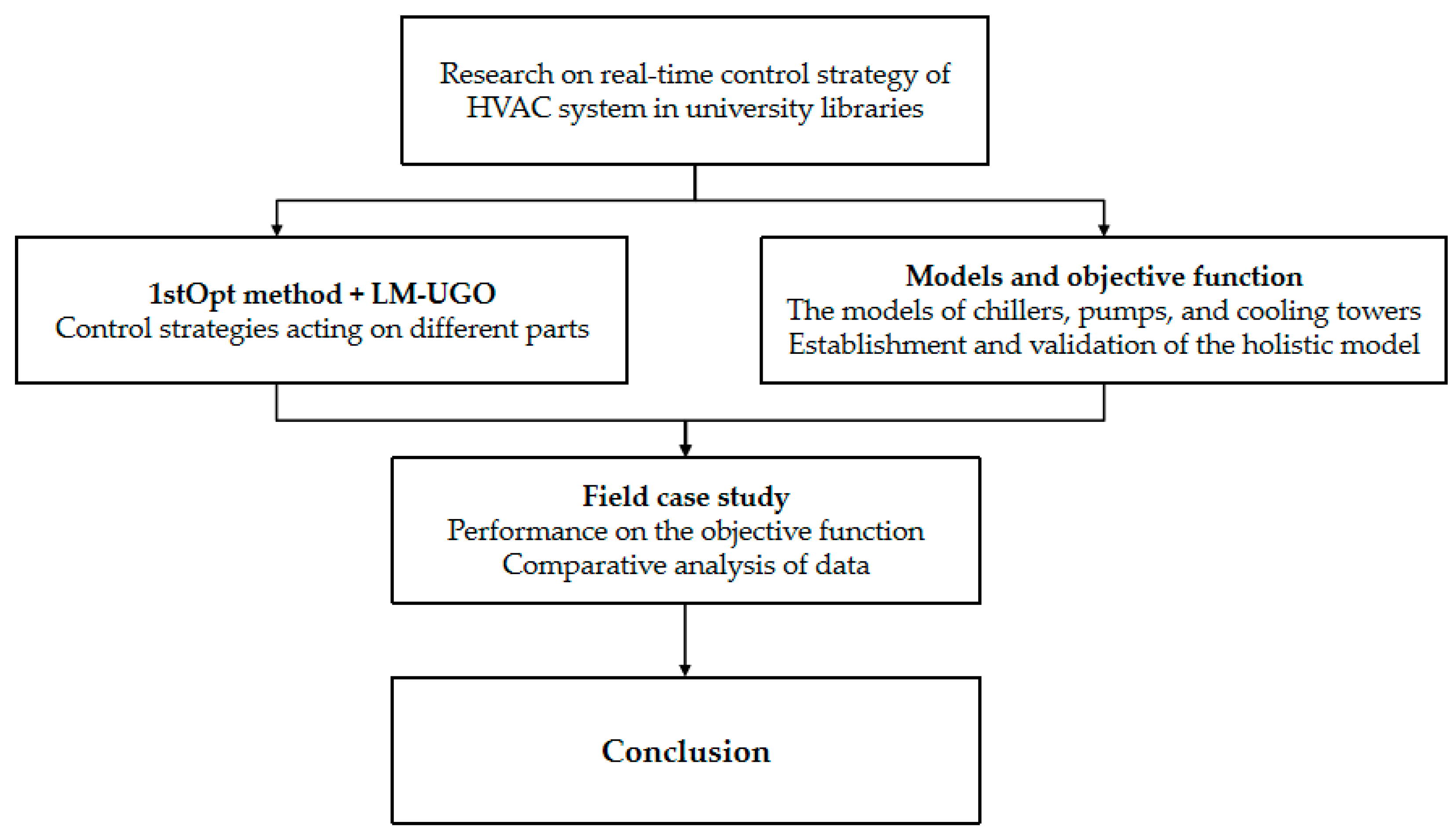
1.3. Overview of the Paper

A significant amount of work has been conducted by previous researchers in the field of HVAC control. This study aims to analyze the current research status of the optimal control of HVAC systems and apply the LM-UGO to develop an optimal control strategy for building HVAC systems. The optimization effect of the algorithm on the objective function model is analyzed, and the algorithm model is applied to a comprehensive HVAC system control model. Finally, an intelligent control scheme for the HVAC system is proposed, which can be applied in the development of more sustainable buildings.

The structure of the study is shown in Figure 1. The main contributions include discussing the performance of an integrated control strategy for overall energy models under daily operating conditions, applying the control model to a library building’s HVAC system, and analyzing and comparing daily energy consumption data to verify its potential for energy savings.

2. Materials and Methods

In this section, we first describe the control strategy method used in building HVAC systems and then introduce the algorithm of the control model.

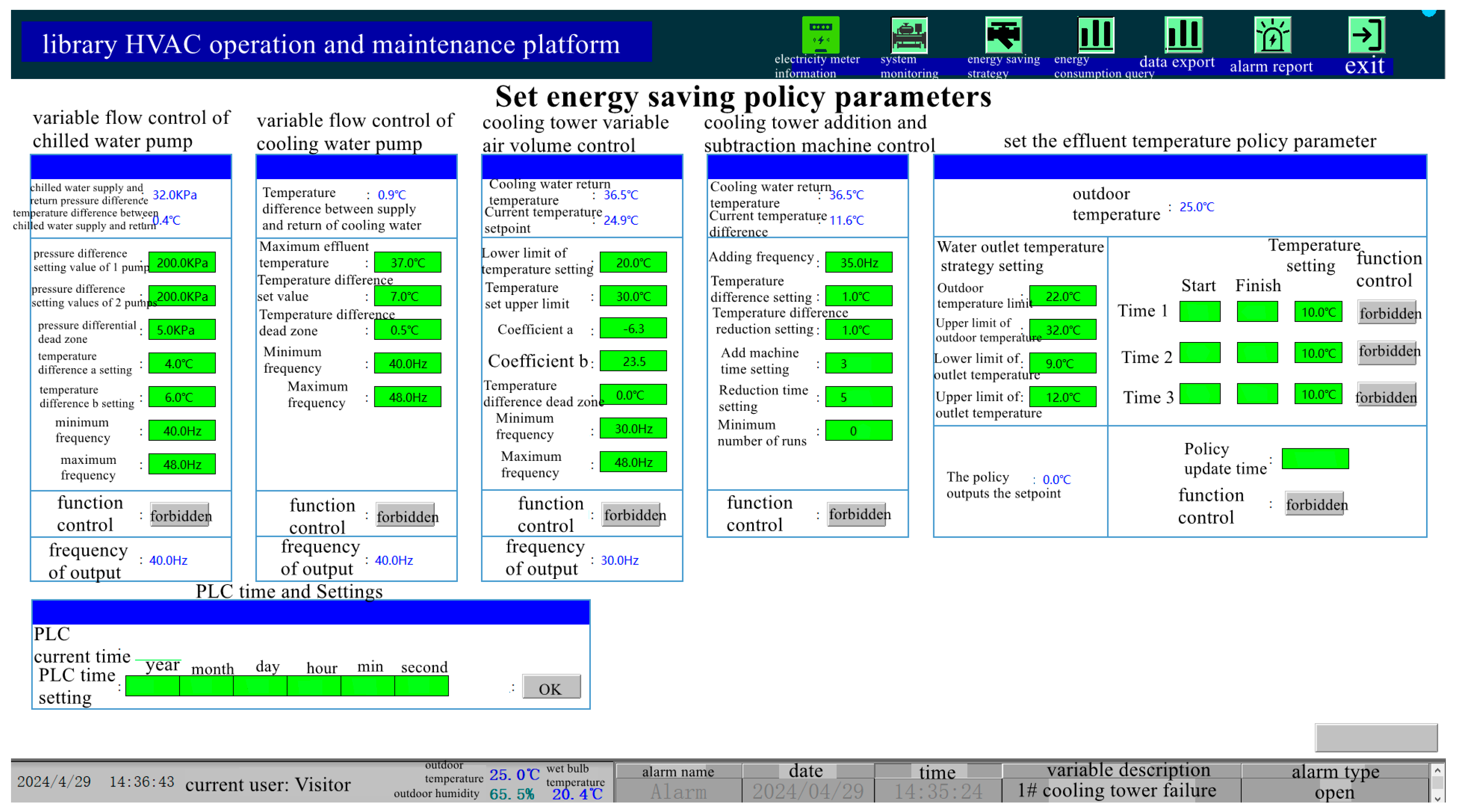
2.1. Energy-Saving Strategies

The energy-saving strategy design is based on the intelligent on-demand regulation of the central HVAC system equipment according to the cooling demand of the HVAC area of the building, as well as the real-time online optimization of each state point of the system operation according to the meteorological parameters and real-time operation data of the system.

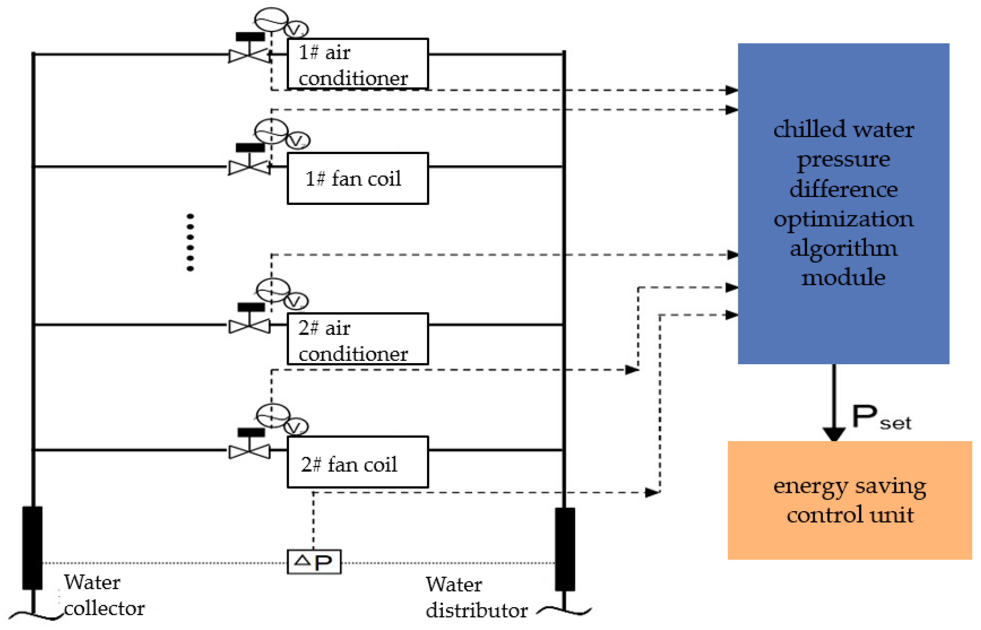
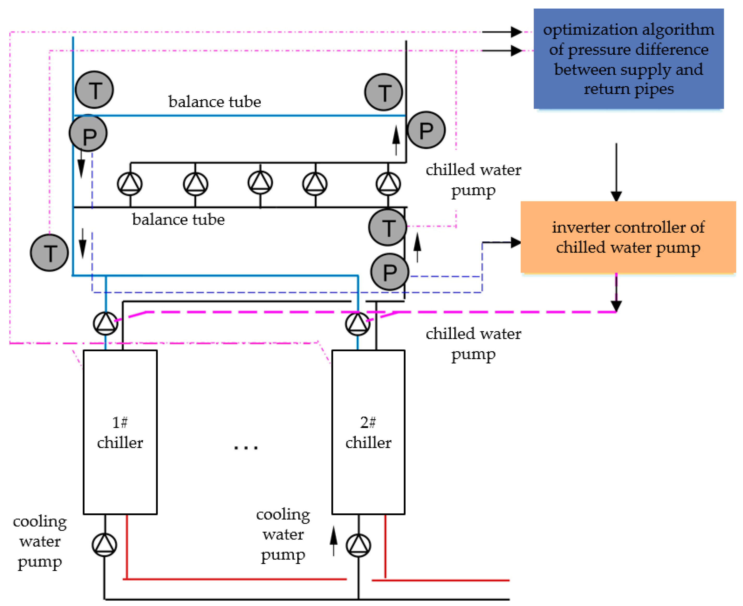
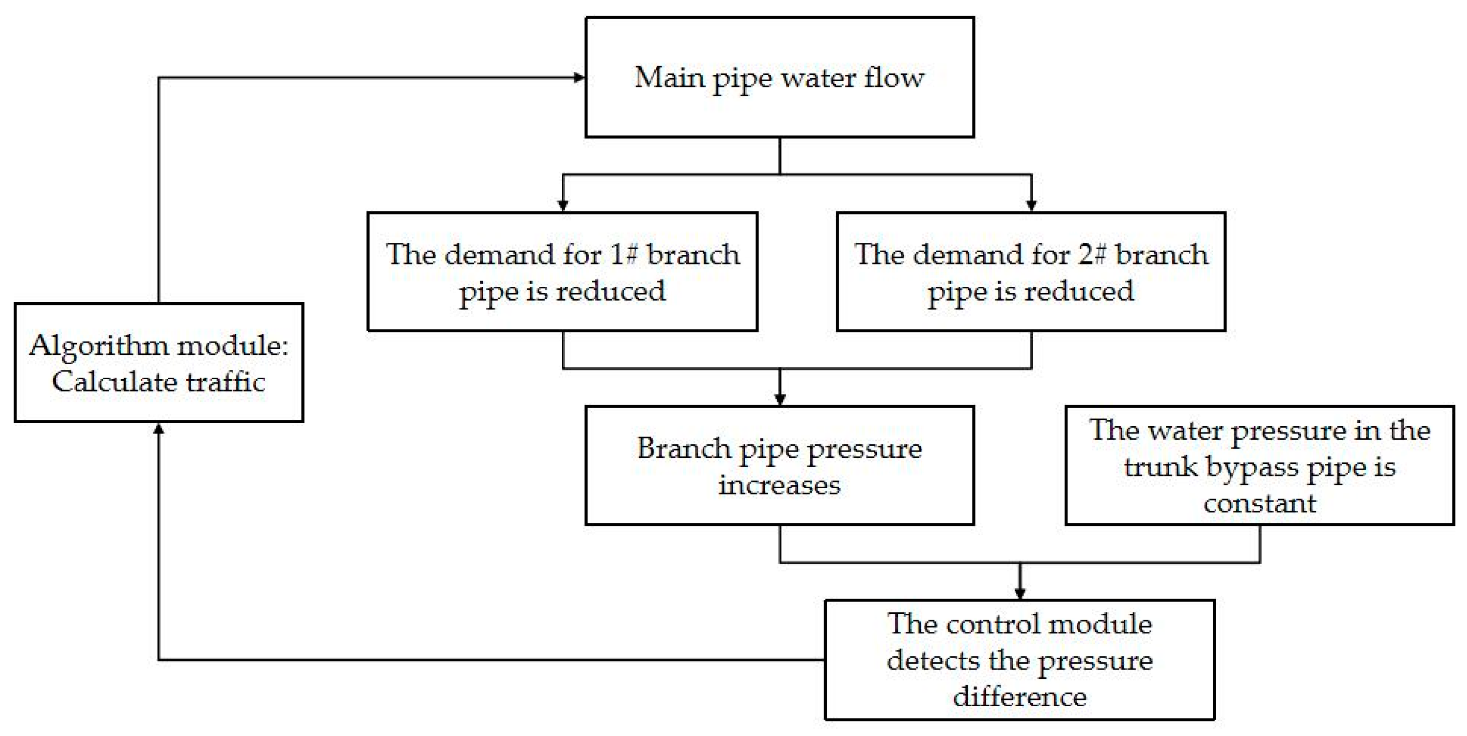
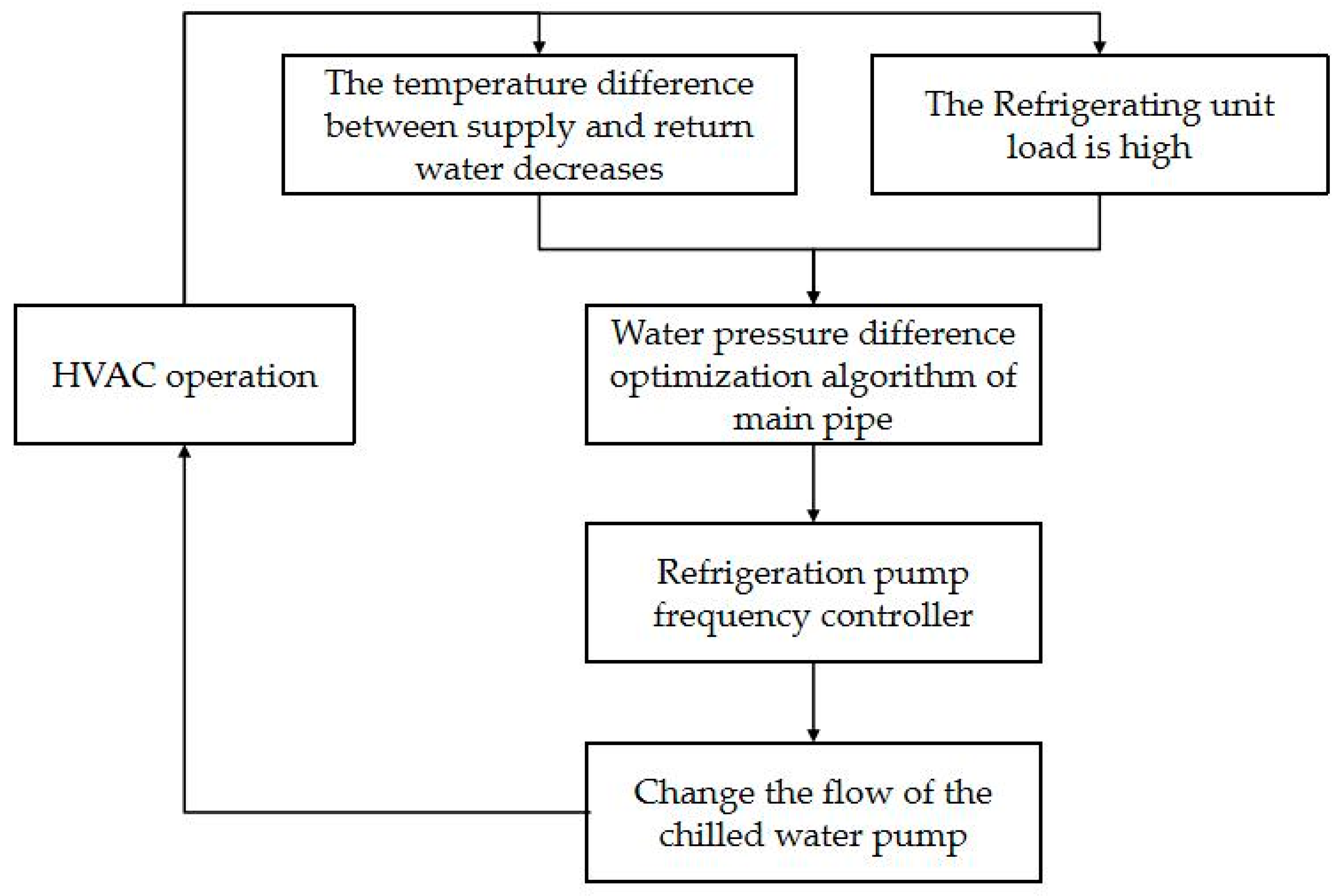
2.1.1. Optimization of Chilled Water Supply and Return Trunk Differential Pressure Setting Based on Weather Change

By collecting data on system operations and changes in terminal load, we can optimize the pressure differential between the chilled water supply and return pipes. This adjustment enables us to achieve energy savings in the operation of the chilled water pumps.

For the secondary pump system, a bypass pipe must be set between the primary and secondary systems to balance the flow between the primary and secondary pumps. However, in the actual operation of the system, the secondary system water flow rate changes with the load. When the load is low, the secondary system water flow rate is small, and because the primary system has a fixed flow rate, the positive flow rate of the bypass pipe is large, resulting in a waste of energy in the primary system. Therefore, for the secondary system, a primary system using a variable-flow design can effectively reduce the operating energy consumption of the system (Figure 2).

For the primary variable-flow system, fixing the differential pressure between the primary system water supply main pipe and the return main pipe can effectively reduce the energy consumption of the primary system; however, when the number of hosts changes, the initially set target value of differential pressure will no longer be applicable. Therefore, it is necessary to optimize the set value of differential pressure according to the temperature difference between the supply and return water of the primary circuit and the current host loading rate; that is, when the temperature difference value is lower and the host loading rate is higher, the differential pressure set value needs to be reduced appropriately in accordance with a certain rule. In other cases, the differential pressure setting value can remain unchanged. Figure 3 shows a structural diagram of the system at the end of the refrigeration unit. Figure 4 presents a basic step diagram of the proposed strategy.

2.1.2. Optimization of Chilled Water Supply Temperature Setpoints Based on Climate Change

The chilled water supply temperature is optimized according to the indoor and outdoor meteorological parameters and system operation data (it is necessary to set the chilled water supply temperature of the unit remotely and automatically through the communication card) to improve the system operation efficiency and minimize the total energy consumption of the chiller unit and primary chilled water pump.

When the HVAC cold load is unchanged, as the chilled water outlet water temperature increases, the power consumption of the chiller unit decreases, and the COP (energy efficiency ratio) of the chiller unit rises by 2–3% for every 1 °C increase in the chilled water outlet temperature. Generally, the optimal chilled water outlet temperature is the chiller-chilled water outlet temperature set value. However, as the HVAC load continues to change, the optimal chilled water outlet water temperature also changes.

In actual operation, the outdoor temperature is used as the basis for setting the chiller-chilled water outlet temperature. When the outdoor temperature rises, the cold load of the system is larger, and dehumidification is also relatively larger; the chilled water outlet temperature is set at a lower value, both to meet the requirements of dehumidification and to meet the system cooling requirements. When the outdoor temperature is low, the cold load of the system is small, the amount of dehumidification is also relatively small, and the chilled water temperature can be set at a higher value. To meet the requirements of the system, dehumidification can also meet the requirements of the cooling system. A higher chilled water temperature can satisfy the system cooling requirements under the condition of consuming less power by the compressor to achieve energy savings. The relationship between the optimal chilled water discharge temperature and outdoor temperature can be adjusted according to the actual operating conditions of the water system.

In actual applications, the optimized chilled water supply temperature is corrected according to the system operation data (mainframe load rate, temperature difference between supply and return water, etc.). In this study, when the load rate of the host was low and the temperature difference between the supply and return water was small, the optimized chilled water supply temperature was increased by the corresponding algorithm; when the load rate of the host was high and the temperature difference between the supply and return water was large, the optimized chilled water supply temperature was reduced by the corresponding algorithm. The energy consumption of the system can be reduced by correcting the optimized chilled water supply temperature to ensure the cooling capacity of the system. Figure 5 shows a basic step diagram of the proposed strategy.

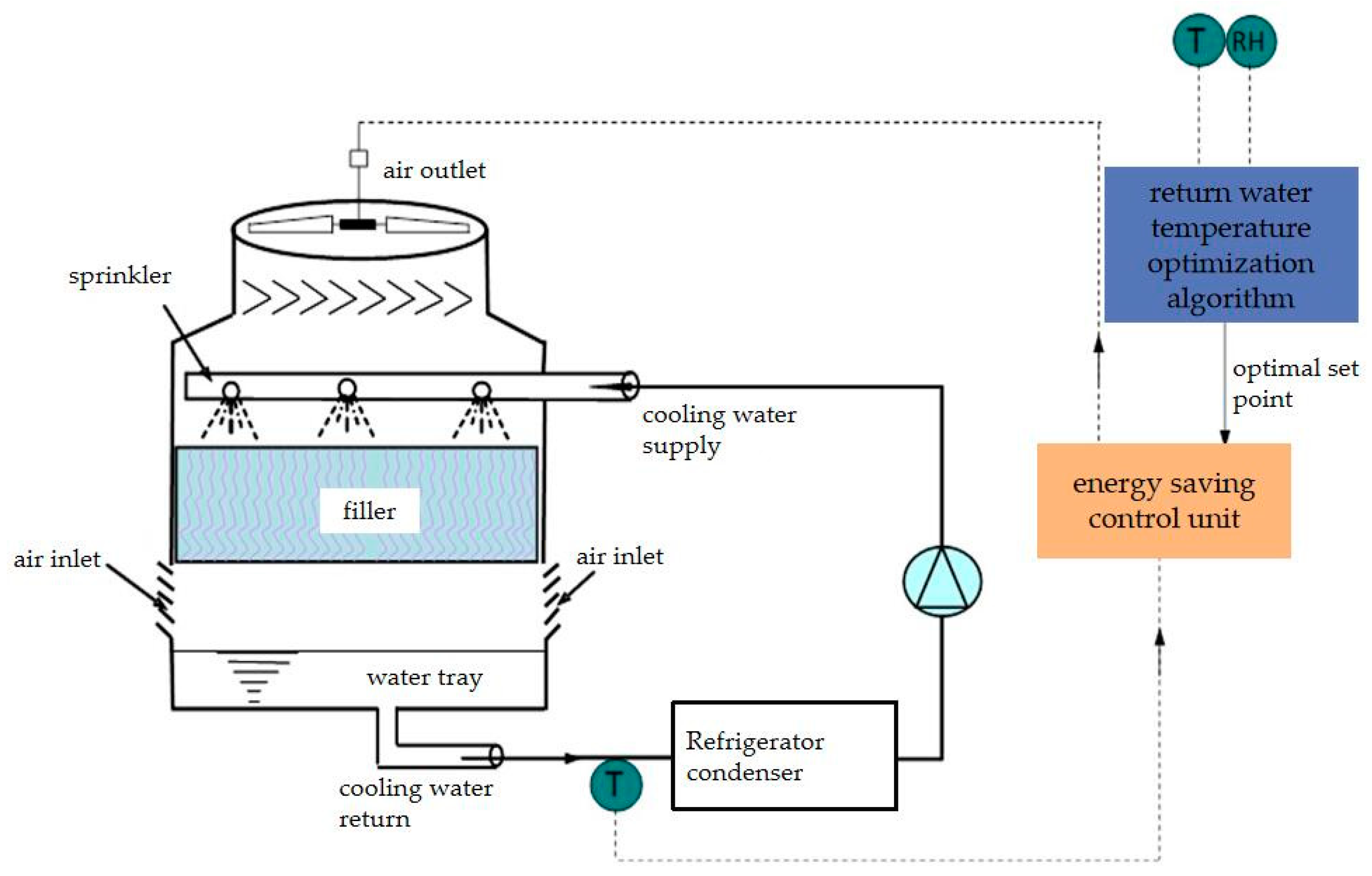
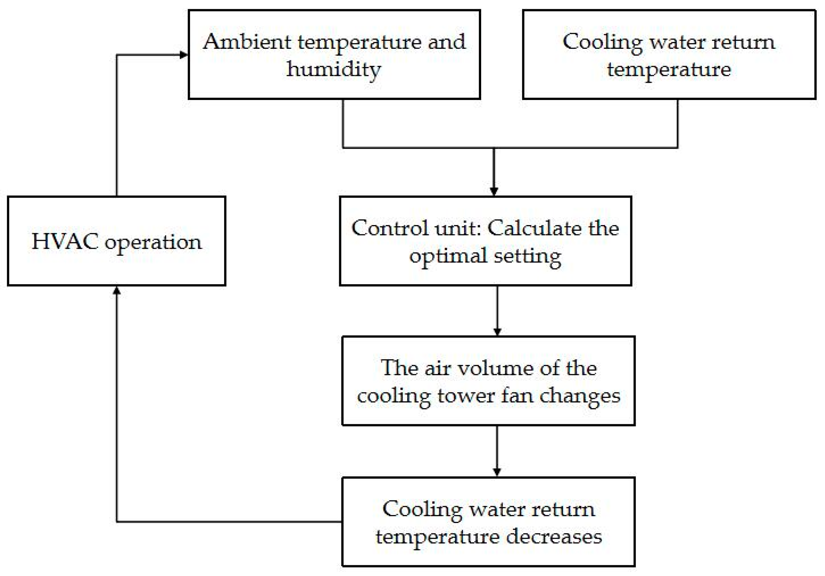
2.1.3. Climate Change-Based Optimization of Cooling Water Return Temperature Setpoints

The cooling water return temperature setting value is optimized according to the outdoor meteorological parameters and system operation data to improve the system operation efficiency so that the total energy consumption of the chiller and cooling tower fan is the lowest.

When the HVAC cold load is constant, the amount of heat removed by the system remains unchanged. When the rotational speed of the cooling tower fan is constantly increasing, the cooling water return temperature is constantly decreasing, which can be infinitely close to the wet bulb temperature. The efficiency of the chiller is improved, and the power consumption is reduced, but the energy consumption of the cooling tower is increased. In contrast, when the cooling tower fan speed continues to decrease, the cooling water return temperature continues to increase, the efficiency of the chiller is reduced, and the energy consumption increases, but the cooling tower energy consumption decreases. Therefore, there is an optimal cooling water return temperature such that the total power consumption of the cooling machine and cooling tower fan is minimized. In general, the optimal cooling water return temperature is the set value of the cooling water return temperature of the chiller. However, with the continuous change in outdoor temperature and humidity, the optimal cooling water return temperature also constantly changes.

The system structure is shown in Figure 6. The outdoor wet bulb temperature is the basis for setting the cooling water return temperature of the chiller. To maintain the cooling water return temperature and the outdoor wet bulb temperature of the approximation (the approximation changes with the change in the outdoor wet bulb temperature, usually 2–4 °C), when the outdoor wet bulb temperature changes, the cooling water return temperature optimization algorithm module calculates the optimal cooling water return temperature setting value and sends it to the energy-saving control unit, which controls the cooling water return temperature by controlling the starting and stopping of the cooling tower fan. Figure 7 shows a basic step diagram of the proposed strategy.

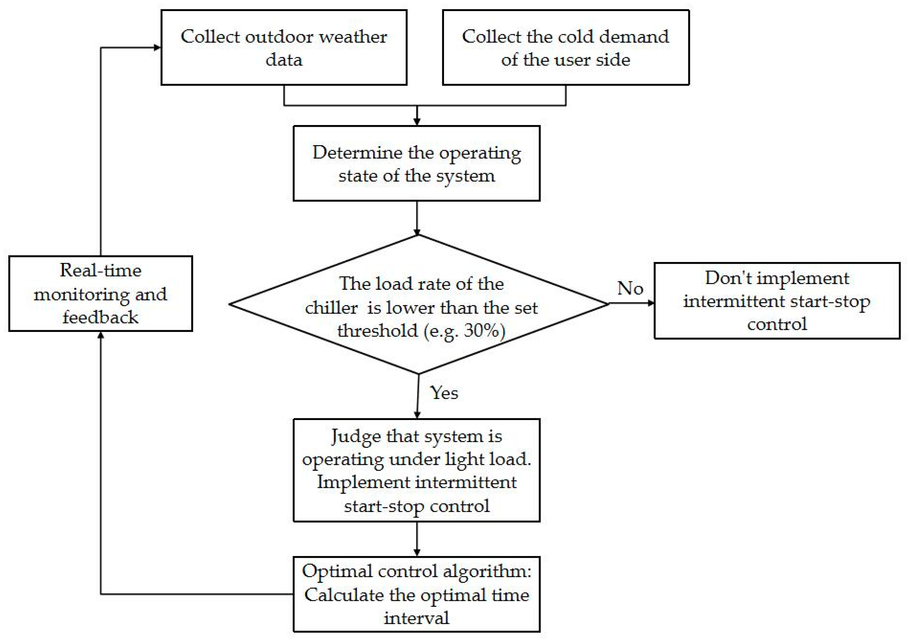
2.1.4. Optimal Control of Intermittent Operation of Small-Load Systems Based on Climate Characteristics

According to the outdoor meteorological parameters and end cold demand, the refrigeration station system implements intermittent start–stop control; that is, when the chiller unit is in small-load operation, the chiller unit, cooling water pumps, and cooling tower use intermittent start–stop control, make full use of the cold stored in the chilled water system, reducing the energy consumed by the system.

Intermittent control refers to the system in accordance with certain rules for intermittent start–stop control. When the water system runs for a period of time, in accordance with the order of priority of the refrigeration unit, cooling water pumps, cooling towers, and chilled water pumps to maintain the operating state, the system stops for a period of time. Then, in accordance with the order of priority, the cooling tower, cooling water pumps, and refrigeration unit start up again. During the night or transitional season, when the HVAC load is low, the refrigeration unit usually operates under low-load-rate conditions, and the operating efficiency is low. After using intermittent control, when the refrigeration unit stops for some time, the chilled water is pumped to the end of the continuous provision of chilled water, and the chilled water temperature gradually increases. When the refrigeration unit starts again, it runs at a higher load factor, and the cooling efficiency is greatly improved. This intermittent operation effectively reduces the operating energy consumption of the refrigeration unit while simultaneously reducing the operating energy consumption of the equipment on the cooling side.

When using intermittent control, it is necessary to determine the stopping time interval and running time interval of the system; if the time interval is not set properly, the thermal comfort of the air-conditioned room will be seriously affected. Therefore, when using intermittent control, the optimal control algorithm should be used to calculate the optimal system running time interval and stopping time interval according to the end load situation to ensure the thermal comfort of the air-conditioned room, increase the stopping time of some of the system equipment as much as possible, and minimize the system’s operating energy consumption. Figure 8 shows a basic step diagram of the proposed strategy.

2.2. LM-UGO Algorithmic

2.2.1. 1stOpt

1stOpt software is a comprehensive tool for mathematical optimization. Analysis software can be connected by a variety of languages (such as C+++, Fortran, Basic) compiled from the external objective function of the dynamic connection library or command executable files, and can be directly read and stored in Excel, CSV, and other formats. This software comes with hundreds of examples covering all aspects of optimization, so it can be used to achieve most objectives including linear and nonlinear fitting and regression; linear, nonlinear, and integer programming; implicit function root solving; graphing; and polarization [27,28].

Its computational platform is characterized by easy and stable operation, powerful functions, and a simple and easy-to-understand interface. It uses the universal global optimization algorithm (LM-UGO), which has a powerful fault tolerance and optimization function and is unique in the fields of nonlinear fitting, parameter estimation, and other optimization [29]. The most important feature of this algorithm is that it overcomes the problem of providing suitable initial values for the use of iterative methods in the field of optimization computation. End-users do not need to give the initial values of their parameters, which are randomly given by the 1stOpt itself, and the optimal solution is finally obtained through its unique global optimization algorithm [30].

2.2.2. LM-UGO

The trust domain algorithm can find the minima without the need for a one-dimensional search step by adjusting the search direction [31]. The confidence domain and one-dimensional search are the same algorithms underlying the optimization algorithm, and the confidence domain algorithm does not involve the one-dimensional search procedure. However, modern confidence domain methods were introduced by Bandeira et al. [32]. He formulated the confidence domain subproblem, a criterion for accepting direction step sk, a criterion for correcting the radius of the confidence domain, and a convergence theorem. These measures make the confidence domain method superior to the line search method.

The LM algorithm is a nonlinear optimization algorithm. The principle of the algorithm is a combination of Newton’s method and the gradient descent method, and its essence is to transform the original problem into multiple LS method problems to be solved during the iterative solving process. The LM algorithm can effectively deal with the redundant parameter problem so that the chance of the cost function falling into the local optimum is greatly reduced [24].

The LM-UGO has powerful fault tolerance and optimization search functions. The most important feature of this algorithm is that it overcomes the difficulty of using the iterative method that must be given a suitable initial value. End-users do not need to give the initial value of its parameters, as these are randomly given by 1stOpt itself, finally arriving at the optimal solution through its unique global optimization algorithm. The goal of ordinary least-squares optimization is to determine the search direction from an initial point and perform a one-dimensional search in that direction. When an acceptable point is found, the search direction is adjusted using certain strategies, and the one-dimensional search continues in a new direction until the objective function is converted to a point of minimal value [33].

2.2.3. Integration of Algorithm Module with HVAC System

Temperature, humidity, flow, and other sensors are connected to the algorithmic control module to collect real-time operating data from the HVAC system. The Modbus RTU communication protocol is adopted to ensure that the sensor data can be stably transmitted to the control module. The PID control and optimization algorithm is embedded into the control module, which is used to process the collected data and generate control instructions. The algorithm module analyzes the collected real-time data and calculates the optimal control strategy according to the preset optimization objectives (e.g., the lowest energy consumption and the best thermal comfort). According to the calculation results of the optimization algorithm, it generates control commands for chiller units, cooling towers, pumps, and other equipment such as start–stop and frequency adjustment, and sends the control commands to the controllers of each item of equipment through the communication interface (e.g., RS485, Ethernet). The operating status of each device is fed back to the algorithmic control module for the real-time adjustment of the control strategy, and the algorithmic module dynamically adjusts the control commands according to the feedback data to ensure that the system always operates in the optimal state. Local or remote user interfaces are developed for the manual intervention of the control strategy and for viewing system status and historical data, and remote monitoring and control are achieved through Wi-Fi, the Ethernet, etc., to support real-time viewing and adjustments to system status. The flowchart is shown in Figure 9.

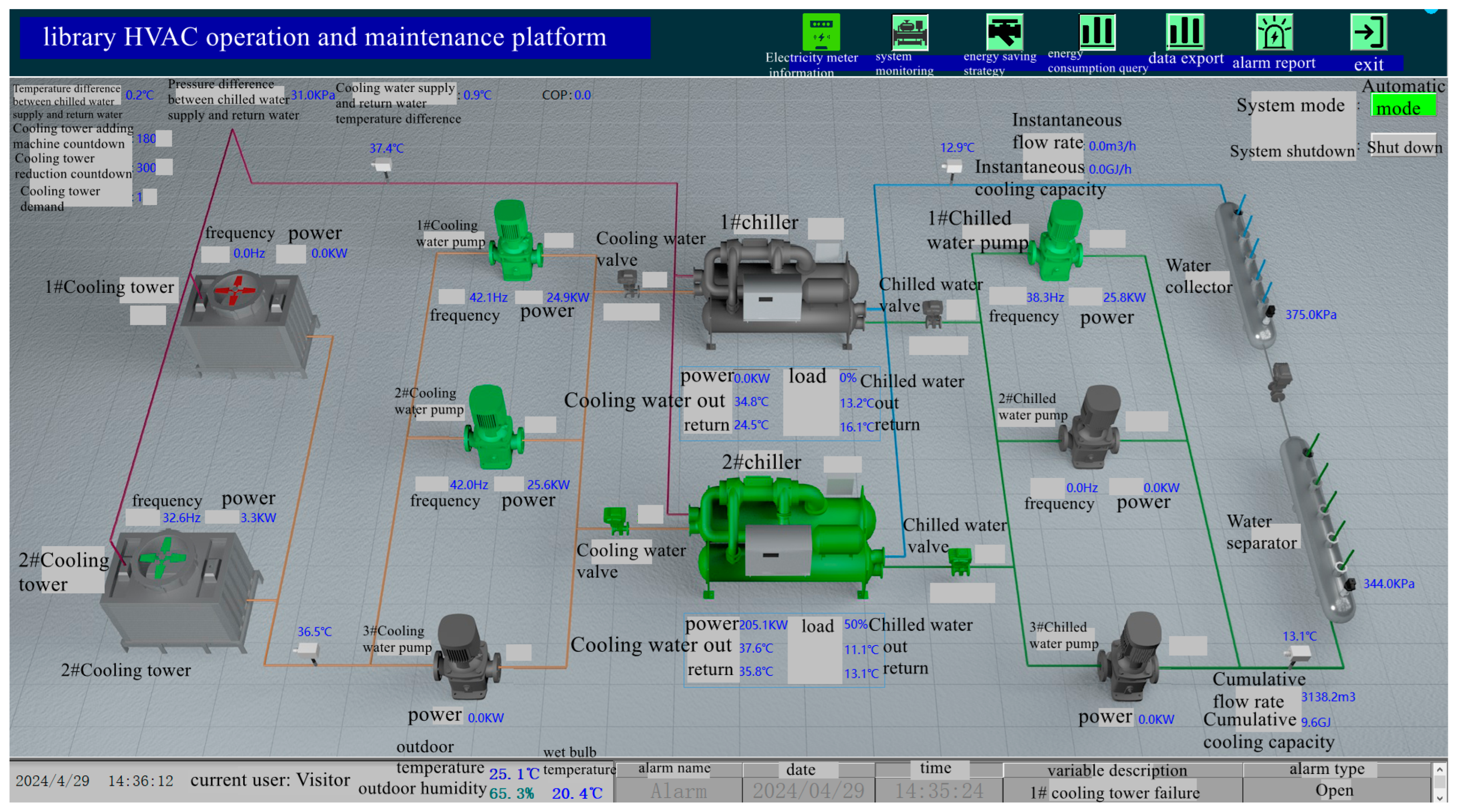
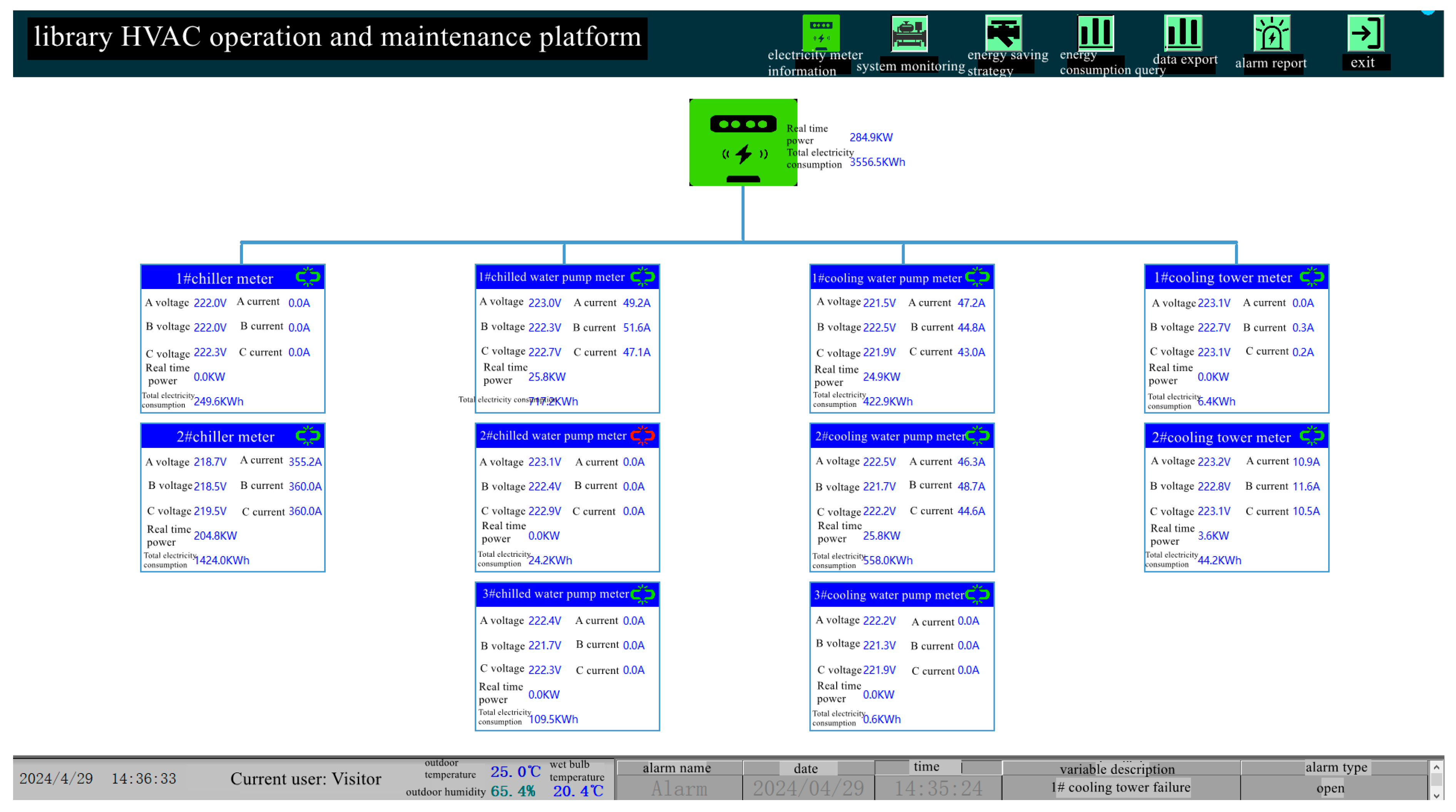
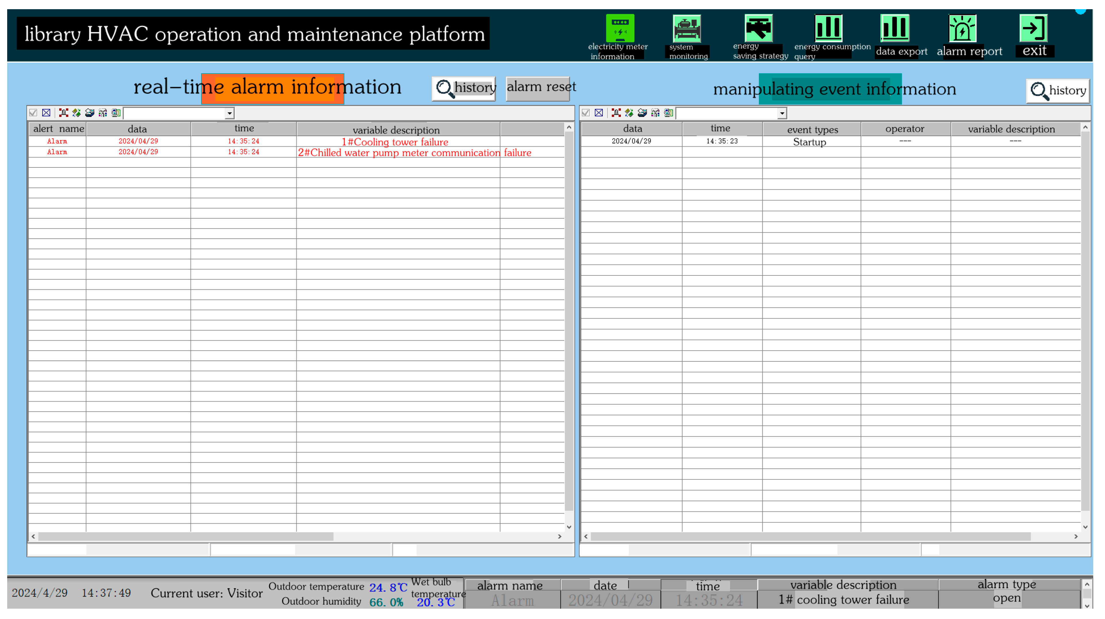
2.3. Operation and Maintenance Platform System

To meet the needs of real-time monitoring and the strategy regulation of HVAC systems, an O&M platform system was built. The system interface has five pages.

The system monitoring page is shown in Figure 10. The main functions are as follows: 1. Display the status of the unit, pump, valve, and other equipment (operation, shutdown, and failure). 2. Adjust the unit, pump, valve, and other equipment switching controls and parameter adjustments. 3. Display real-time data from various types of sensors in the system. 4. Carry out the system of one-key power on and the system of cooling/heating mode switching.

The energy-saving strategy page is shown in Figure 11. The main functions are as follows: 1. Adjustment of the unit time-limited temperature control and seasonal temperature control strategies. 2. Adjustment of the pump control strategy.

The energy consumption query page is shown in Figure 12. The main functions are as follows: 1. Query the historical information on the power consumption of each electrical device (daily and monthly). 2. Export historical information on the power consumption of each electrical device (daily and monthly). 3. Query and export the historical data of each setting parameter and calculation parameters of the system (daily and monthly).

The alarm report page is shown in Figure 13. The main functions are as follows: 1. Query system real-time faults and historical fault information. 2. System operation information records, including account login, equipment switch operation, parameter adjustment, and other operation information.

3. Experimental Cases

This section describes the steps involved in developing, building, and validating the HVAC system model, as well as the collection and visual display of the experimental data.

3.1. Project Overview

The system model was established and applied in the HVAC system of a university library building in Hubei Province. As shown in Figure 14 and

Table 1. Equipment parameters.

Equipment Type	Parameters	Quantity
Chiller	Rated cooling capacity 2040 kW, rated power 361.7 kW	2
Chilled water pump	Rated flow 466 m3/h, rated power 55 kW	3
Cooling water pump	Rated flow 466 m3/h, rated power 45 kW	3
Cooling tower	Motor power: 11 kW Flow rate: 900 m3/h	2

, the system consists of two chillers, three chilled water pumps, three cooling water pumps, and two cooling towers. The chilled water pumps are connected in parallel, while the cooling water pumps are connected in series with the cooling towers and chillers. The water flow data and temperature data of each part are collected by the corresponding sensors. Some of the cooling water pumps and chilled water pumps are kept off standby when the HVAC cooling system supply meets the demand. The standby cooling water pumps are connected to the first freezer and are arranged in a series configuration with the cooling tower and the freezer.

3.2. Device Model and Objective Function

We built chiller and pump models to accurately model the HVAC systems. The data required for modeling were collected from a university library project in Hubei Province. In total, 80% of the data were used for modeling, and the remaining 20% were used for validation.

3.2.1. Chiller Model

The coefficient of performance of the cooler can be expressed as follows:

$$COP={\displaystyle \frac{r}{\left(\frac{t_{\mathrm{o}}+273.15}{{\mathrm{t}}_{\mathrm{v}}+273.15}-1\right)r+z_1\frac{t_{\mathrm{o}}+273.15}{{\mathrm{t}}_{\mathrm{v}}+273.15}-z_2}}$$

(1)

where r is the load rate of the chiller, representing the condensing temperature (°C); tv is the evaporating temperature (°C); and z₁ and z₂ are the parameters to be determined.

$${\mathrm{t}}_o=t_{w,o,E}+{\displaystyle \frac{Q_o}{c_w{G}_{w,o}(1-e^{-\frac{U{A}_o}{c_w{G}_{w,o}}})}}$$

(2)

$${\mathrm{t}}_v=t_{w,v,E}+{\displaystyle \frac{Q_v}{c_w{G}_{w,v}(1-e^{-\frac{U{A}_v}{c_w{G}_{w,v}}})}}$$

(3)

$$Q_o=c_w{G}_{w,o}(t_{w,o,E}-t_{w,o,L})$$

(4)

$$Q_v=c_w{G}_{w,v}(t_{w,v,E}-t_{w,v,L})$$

(5)

Here, c_w is the specific heat capacity of water. t_o and t_v are determined by the inlet water temperature of the chiller and the heat exchange between the condenser and the evaporator. t_o is determined by the outlet temperature of cooling water t_w,o,E (°C) and the cooling water flow rate G_w,o (kg/s). t_v is determined by the outlet temperature of the chilled water, t_w,v,E (°C), and the chilled water flow rate G_w,v (kg/s). t_w,o,L (°C) is the inlet temperature of the cooling water, and t_w,v,L (°C) represents the inlet temperature of the chilled water. U_Ao and U_Av represent the total heat-transfer coefficients (W/°C) of the condenser and evaporator, respectively.

The power of the chiller is a function of the cold load, chilled water outlet temperature, and chilled water flow rate as the input parameters.

$$P_{chiller}={\displaystyle \frac{Q_e}{COP}}$$

(6)

Q_e represents the chilled load (kW) and is calculated based on the last chilled water flow (G_w,e) and supply and return water temperature (t_w,v,e, t_w,v,L) difference, as follows:

$$Q_L^T={\mathrm{c}}_{\mathrm{w}}{G}_{w,e}^{T-1}(t_{w,v,E}^{T-1}-t_{w,v,L}^{T-1})$$

(7)

3.2.2. Cooling/Chilled Water Pump Model

The pump power and flow rate are fitted through the following equations:

$$P_{\mathrm{p}}=b_0{G}_w^2+b_1{G}_w+b_2$$

(8)

where P_p represents the pump power, b₀, b₁, and b₂ represent the pump site data obtained by least-squares fitting, and G_w represents the water flow rate (m³/h). The chilled water pumps in parallel, and the average temperature, t_m (°C), can be calculated according to the following formula:

$$t_m={\displaystyle \frac{{\displaystyle \sum c_w^i{t}_w^i}}{{\displaystyle \sum c_w^i}}}$$

(9)

In the formula, c_w represents the specific heat capacity of water (J/(°C∙kg)) and t_w represents the water temperature (°C).

3.2.3. System Model and Boundary Conditions

The energy consumption of the entire HVAC system is modeled using the above model of pumps and chillers with the objective function.

$$\begin{array}{l}{P}_{xyz}=P_{system}\\ ={\displaystyle \sum P_{\mathrm{chiller}}^{i1}}+{\displaystyle \sum P_{\mathrm{chillerwaterpump}}^{i2}+{\displaystyle \sum P_{\mathrm{coolingwaterpump}}^{i3}}}\\ =F(Q_L,t,hu,G_{w,o}{T}_{w,v,L})\end{array}$$

(10)

In this function, the cooling load Q_L, temperature t, and humidity hu are the input parameters that agree with the actual situation, whereas G_w,o and T_w,v,L are the parameters to be adjusted. When these parameters are determined, other required physical quantities can be obtained according to the conservation of mass and energy. The P_chiller can be calculated using Equations (1) and (6), while the chilled water pump power and cooling water pump power can be calculated using Equation (8). The objective of the optimization algorithm is to determine the appropriate G_w,o and T_w,v,L to minimize the energy consumption of the system.

The energy consumption of the HVAC system was calculated as shown in Equation (10). After sensing the parameters Q_L, t, and hu, the current chilled water inlet temperature and set chilled water output temperature were utilized to calculate the chilled water flow rate, power consumption, and evaporative temperature of the chiller t_e. The chilled water flow rate, power consumption, and cooling tower energy consumption were calculated based on the current chilled water flow rate. The chiller power consumption was obtained by iteratively calculating the evaporation temperature based on the circulating chilled water flow rate and determining the condensation temperature. Finally, the power consumption of the entire system was obtained using the current parameter settings.

In the algorithmic control module of an HVAC system, the equations of conservation of mass and conservation of energy are indispensable tools in the modeling and optimization process. Not only do these equations help to ensure that the physical processes of the system conform to the basic laws of physics as constraints for the optimization algorithms to ensure that the flow rate of the system remains balanced during operation, but they also allow for the calculation of cooling and chilled water flow rates based on known flow rates or pressure differentials and the detection of leaks or other anomalies in the system through the monitoring of flow rate variations, amongst other uses.

3.2.4. Collection of Equipment Data

To gather data for the experimental research, a communication card was installed on the frequency converter of the unit to facilitate communication between the frequency converter and the upper computer system. The communication card can collect various data during the operation of the frequency converter, including the input voltage and current, output voltage and current, power, temperature, and other parameters. These data can be used to evaluate the operating status of the refrigeration unit, detect anomalies in a timely manner, and make the necessary adjustments. In the HVAC system, sensors are utilized to collect information, such as temperature and humidity, which are then transmitted to the control system. This collected information serves two purposes: it can provide feedback for control adjustment within the HVAC system while also enabling energy consumption calculations based on these data. Some of the devices used are listed in

Table 2. Device information.

Name	Brand	Type	Range and Accuracy
Data collector	Qingdao Hantai	DAQ4090A	Basic DCV accuracy of 0.003%, scan rate up to 450 channels/second
Edge computing gateway	Beijing Hailin	HNE	Temperature measurement accuracy is ±1 °C. The measurement accuracy of voltage and current is ±1%. Measurement accuracy of pressure and flow rate is ±1%
Industrial intelligent gateway	Huachen Zhitong	HINET	Support Ethernet, serial port, CAN port, 10 port and other devices access and Ethernet, 2G/3G/4G full network access. Embedded a variety of industrial protocols, support more than 99% of PLC and most industrial equipment access.
Temperature sensor	TE Connectivity	20011957	Temperature measurement accuracy is ±1 °C. Measuring range is 0 to 50 °C. Temperature measurement accuracy is ±1 °C. Measuring range is 0 to 50 °C.
Humidity sensor	Amphenol	Telaire RH	Measurement range is 5 to 95% RH. Accuracy ±5% RH

.

4. Results and Discussion

4.1. Energy Consumption

The central HVAC system of the University library was scheduled to be opened officially in June 2024. At the beginning of the month (1 June to 6 June), the system was operated for a short period of time (less than 8 h) owing to the low temperatures. After 7 June, as the temperature continued to rise, the HVAC system operated on a fixed schedule, generally from 8:00 to 20:00 every day with some adjustments in operating times. The operating conditions of the entire system can be categorized into four stages: low-load mode (less than 8 h per day), energy-saving mode, original mode, and equipment failure period. The specific operating conditions of each mode are listed in

Table 3. Operating modes.

Equipment Running Time		9:00–17:00	9:00–17:00
Operation Mode		Original Mode	Energy-Saving Mode
Chiller	Number of enabled devices	1	Same as the day before
	Effluent temperature setting	7 °C	Automatic mode
Chilled water pump	Number of enabled devices	2	Automatic mode
	Operating frequency	50 Hz	Automatic mode
Cooling water pump	Number of enabled devices	2	Automatic mode
	Operating frequency	50 Hz	Automatic mode
Cooling tower	Number of enabled devices	2	Automatic mode
	Operating frequency	50 Hz	Automatic mode

.

The statistical data table is organized according to the operation of the system. The actual operational data of the system are shown in Figure 15 and

Table 4. HVAC system energy consumption data from 1 to 23 June.

Data	Mean Outdoor Temperature (°C)	Operation Mode	1# Chiller (kWh)	2# Chiller (kWh)	1# Chilled Water Pump (kWh)	2# Chilled Water Pump (kWh)	3# Chilled Water Pump (kWh)
1 June 2024	26.4	Low-load mode	1003.2	0	112.23	103.44	0
2 June 2024	27.7		0	820.8	95.67	88.29	0
3 June 2024	28.3		1824	0	201.84	185.34	0
4 June 2024	26.3		483.2	0	55.14	50.64	0
5 June 2024	24		0	0	0.75	0.78	0
6 June 2024	25.6		560	0	61.5	56.34	0
7 June 2024	27.3	Energy-saving mode	2443.2	0	273.21	249.57	0
8 June 2024	29.2		2035.2	0	217.2	199.11	0
9 June 2024	26.5		0	1840	228.9	209.13	0
10 June 2024	25.8		1856	0	216.51	197.61	0
11 June 2024	28.6		0	2193.6	223.29	203.7	0
12 June 2024	31.4		2438.4	0	228.48	208.59	0
13 June 2024	32.5	Energy-saving mode	3209.6	0	272.1	248.28	0
14 June 2024	33		0	3422.4	265.5	242.13	0
15 June 2024	33.9	Original mode	3870.4	16	524.88	482.67	0
16 June 2024	32.2	Equipment failure period 1	0	2240	183	167.22	0
17 June 2024	30.4		627.2	0	52.83	48.39	0
19 June 2024	29.6	Energy-saving mode	0	3020.8	278.79	254.46	0
19 June 2024	27.7		0	2694.4	250.62	228.78	0
20 June 2024	27.6		2592	0	260.88	238.44	0
21 June 2024	29.7	Original mode	3828.8	0	498.75	458.79	0
22 June 2024	27.4		3900.8	0	612.42	563.76	0
23 June 2024	27.5	Energy-saving mode	2260.8	0	236.4	215.97	0
1#	2#	3# Cooling water pump (kWh)	1# Cooling tower (kWh)	2# Cooling tower (kWh)	Total (kWh)	1#	2#
Cooling water pump (kWh)	Cooling water pump (kWh)					Mean indoor temperature (°C)	Mean indoor temperature (°C)
104.37	111.96	0	22.81	20.17	1478.18	25.2	25.6
88.56	95.31	0	18.32	15.92	1222.87	25.3	25.8
187.56	200.94	0	37.48	33.41	2670.57	24.9	25.8
51.99	54.84	0	12.23	10.19	718.23	25.4	25.8
0.81	0.75	0	0.37	0.34	3.8	25.3	25.4
58.08	61.32	0	13.24	11.3	821.78	25.2	25.6
257.1	272.43	0	57.01	51.85	3604.37	24.5	25.4
206.43	216.87	0	52.45	47.36	2974.62	24.3	25.6
215.79	226.74	0	40.33	36.4	2797.29	23.9	25.4
205.32	214.68	0	47.45	42.96	2780.53	24	25.2
187.23	201.51	0	66.97	61.18	3137.48	24.3	25.4
197.55	202.53	0	76.57	70.09	3422.21	24.6	25.8
227.13	245.94	0	99.54	90.71	4393.3	24.5	26.1
221.52	239.43	0	100.5	91.86	4583.34	24.7	26.4
202.23	484.86	274.5	104.73	82.29	6042.56	25.1	26.6
0.81	108.69	421.5	67.71	61.17	3250.1	25.5	26.8
49.29	48.78	33.3	18.47	16.11	894.37	26.8	27.4
237.63	244.23	0	106.86	97.34	4240.11	25.8	27.2
215.28	221.19	0	94.19	86.16	3790.62	25.4	26.7
226.92	232.89	0	89.61	82.17	3722.91	25.1	26.3
444.93	458.55	0	86.94	71.35	5848.11	25.1	26.3
548.76	562.35	0	100.91	93.93	6382.93	23.2	25.7
204.3	209.94	0	62.76	57.22	3623.39	23.1	25.6

¹ Equipment failure period: Equipment commissioning and replacement operations are carried out during this operation mode.

.

The original plan was to test the energy-saving effect of the system from 18 June to 22 June, in accordance with the national standard GB/T 31349-2014 [34] “Technical requirements of measurement and verification of energy savings—Central air conditioning system” using the similar day comparison method. However, owing to sudden equipment failure during the operation, the test was interrupted and forced to stop. Although the energy-saving data from this project cannot be strictly verified according to the test standards, the actual operation data still reflect the energy-saving performance of the system to a certain extent. Therefore, this report only presents our self-test data, and the actual energy-saving effect test is subject to a subsequent three-party energy-saving report.

Samples from the low-load period and equipment failure period were excluded. The target samples were selected from the remaining energy-saving mode period and the original mode period. The target samples on similar days must meet specific requirements, as outlined in

Table 5. Requirements for environmental parameters.

Parameter	Mean Daily Outdoor Temperature	Mean Daily Indoor Temperature
Maximum allowable deviation for similar days	±1 °C	≤26 °C

.

The samples were collected on the 18th, 21st, 22nd, and 23rd days in accordance with the testing requirements.

Subsequently, the data were further segmented to extract the daily operational data from 9:00 to 17:00, as shown in

Table 6. Experimental sample conditions and energy consumption.

Name	Data	Operation Mode	Mean Outdoor Temperature (°C)	1# Mean Indoor Temperature (°C)	2# Mean Indoor Temperature (°C)	Energy Consumption from 9 to 17 (kWh)
Sample1	18 June 2024	Energy-saving mode	29.6	25.8	27.2	3021
	21 June 2024	Original mode	29.7	25.1	26.3	5190
Sample2	23 June 2024	Energy-saving mode	27.5	23.1	25.6	5244
	22 June 2024	Original mode	27.4	23.2	25.7	3247

.

Based on the calculations for the above samples,

Table 7. Comparison of energy consumption data.

Name	Data	Operation Mode	Daily Energy Consumption (kWh)	Energy Savings (kWh)	Energy-Saving Ratio (%)
1	18 June 2024	Energy-saving mode	3021	2169	41.79%
2	21 June 2024	Original mode	5190
3	23 June 2024	Energy-saving mode	3247	1997	38.08%
4	22 June 2024	Original mode	5244

illustrates the energy-saving rate of the project.

In conclusion, the initial findings indicate that the overall energy-saving rate of this project exceeded 35%.

4.2. Cost-Benefit Analysis

4.2.1. Cost Recovery

According to the Industrial and Commercial Electricity Price Adjustment Plan for the project issued by the local government, the electricity price for industrial and commercial users was divided into four stages of electricity consumption, as illustrated in

Table 8. Electricity prices at different times.

	Period Division		Electricity Price Coefficient
First stage	0:00–6:00, 12:00–14:00		0.48
Second stage	6:00–12:00, 14:00–16:00		1
Third stage	16:00–20:00, 22:00–24:00 (July and August)	16:00–18:00, 20:00–24:00 (Other months)	1.49
Fourth stage	20:00–22:00 (July and August)	18:00–20:00 (Other months)	1.8

.

According to the “Electricity Law of the People’s Republic of China” issued by the national government, the commercial electricity price is categorized into four price ranges (with a conversion ratio of USD to CNY of 7.177), as shown in

Table 9. The four electricity price ranges.

	Period Division	Electricity Price (US Dollar)
First stage	≤1 kV	0.1055
Second stage	1–35 kV	0.1028
Third stage	35–110 kV	0.1021
Fourth stage	≥110 kV	0.1

.

Hubei Province, located in the central region of China, typically operates its HVAC cooling system for three months during summer. The electricity cost was calculated at a unit price of USD 0.1055 (CNY 0.7577) per kilowatt-hour. The statistics show that the HVAC system runs for 8 h each day from 9 o’clock to 17 o’clock. The HVAC system in the library building can save approximately USD 19,700 per year in electricity costs through energy conservation measures.

4.2.2. Long-Term Return on Investment

The return on investment (ROI) formula was used to evaluate the long-term economic benefits:

$$ROI={\displaystyle \frac{I_{\mathrm{i}}-I_{\mathrm{c}}}{I_{\mathrm{c}}}}\times 100\%$$

(11)

In Equation (11), I_i represents the investment income and I_c represents the investment cost.

The return on investment includes savings on electricity costs and other potential benefits (e.g., longer equipment life, lower maintenance costs). Assuming an initial investment of USD 100,000, the annual savings in electricity costs would be USD 19,700, and the expected lifetime of the energy efficiency measures would be 10 years. This results in a total return of USD 197,000 and a lifetime ROI of 97%.

4.2.3. Policy Incentives

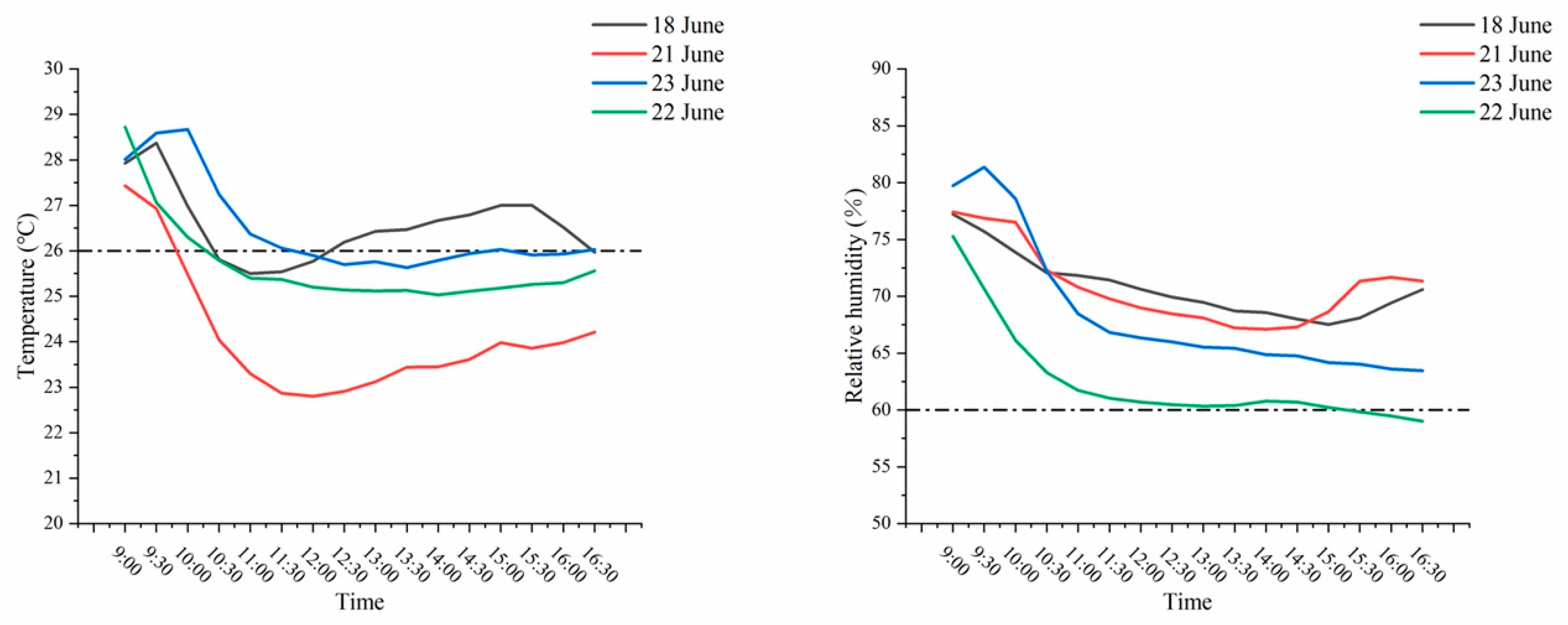
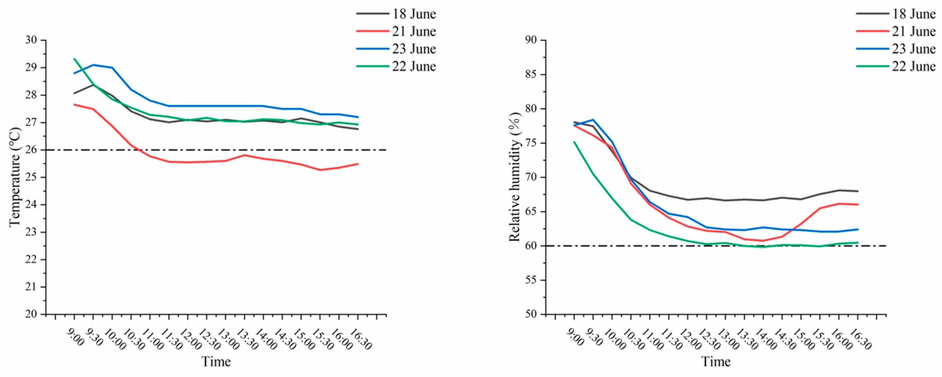
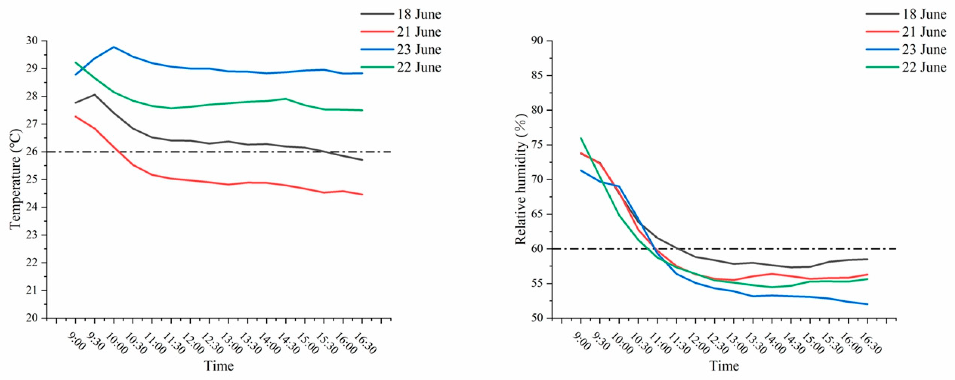
Local governments in Hubei Province provide subsidies for energy-saving projects, and enterprises can enjoy a certain amount of financial support. In addition, according to the Electricity Law of the People’s Republic of China, school libraries can enjoy preferential electricity prices for adopting energy-saving measures. These policy incentives can accelerate investment recovery and improve return on investment.

With the gradual improvement in the carbon emissions trading market, library energy-saving programs can gain additional revenue by reducing carbon emissions. Through energy-saving measures, school libraries can not only reduce operating costs but also improve the competitiveness of the school itself. Government policy incentives can accelerate the promotion and application of energy-saving technologies and promote sustainable development.

4.3. User Comfort

In the standard specification GB 50189-2015 [35] “Design standard for energy efficiency of public buildings”, it is mentioned that the design of air conditioning systems in public buildings should meet the comfort requirements of indoor temperature and humidity. For example, for an air conditioning system with independent control of temperature and humidity, it is necessary to select appropriate dehumidifying methods and temperature sources to ensure that the indoor humidity is within a comfortable range. In addition, GB 55016-2021 [36] “General code for building environment” clearly states that the building environment should meet the basic requirements of human health for sound, light, thermal environment, and air quality, including the reasonable control of indoor temperature and humidity.

To understand the temperature and humidity control of the library HVAC system, an experiment was conducted to detect temperature and humidity data in the user reading area on the first floor of the library.

Five test points were established in the test area; their locations are shown in Figure 16. The experiment used a TES-1341 electronic breeze meter (Manufacturer: Taiwan Taishi, place of origin: Shenzhen, China) for data measurement, which included wind speed, temperature, relative humidity, and other relevant data. The equipment was positioned on a tripod at a height of 1.5 m above the ground, as shown in Figure 17. The measuring instrument was operated in automatic mode, collecting data at 5 min intervals. According to the comparison principle in Section 4.1, 18 and 21 June and 22 and 23 June were selected for comparison in the experiment. The data were extracted, and the temperature change curve and relative humidity change curve of the test points (A-E) were drawn, as shown in Figure 18, Figure 19, Figure 20, Figure 21 and Figure 22.

As can be seen in the graphs of the data from the individual test points, both the temperature and relative humidity initially rose during the morning hours in original mode. This indicates that the cooling capacity of the unit in this mode was insufficient to meet the demands of the increased library staff and higher outdoor temperatures. However, after retrofitting the HVAC system with an energy-saving mode, the unit was able to provide sufficient cooling capacity to adapt to changes in external factors and meet the temperature requirements of library users. In accordance with GB 50189-2015 [35] “Design standard for energy efficiency of public buildings”, the indoor temperature of the library building is set at 26 °C in air conditioning mode. Compared to the original model, the indoor temperature after the energy efficiency retrofit is closer to the temperature value set by the specification, thus, creating a good temperature environment for library users more quickly. In GB 55016-2021 [36] “General code for building environment”, the relative humidity of indoor air should be taken as 60% as the design reference value. According to the data in the figure, the relative humidity value after the energy-saving renovation was closer to the design reference value than in the original mode.

The comparison of different measurement points revealed variations in temperature and humidity across different regions, which may be attributed to factors such as the building’s external wall material and exposure to sunlight. This aspect warrants further investigation and potential modifications. By examining the functional use of various regions, as well as considering external wall materials and other relevant factors, adjustments can be made to control the strategies and methods for each specific region.

4.4. Limitations of the Method

Compared with other algorithms, the LM-UGO offers several advantages. It demonstrates a fast convergence speed and avoids becoming trapped at the local minimum points. In addition, it enables the total error of the system to quickly reach the required accuracy level, has a short training time, and provides more accurate data prediction. The LM-UGO also exhibits strong fault tolerance and high reliability. In scenarios with multiple influential factors (i.e., more input nodes), the network prediction established by the LM-UGO achieved high accuracy and rapid speed, making it suitable for applications with stringent real-time requirements. Therefore, the LM-UGO has promising prospects for application. However, owing to its substantial computational and storage requirements, a relatively high-performance computer is necessary when utilized in large complex networks. Moreover, when excessive weight is involved, the applicability of the LM algorithm may not be guaranteed; therefore, further research is required.

The findings of this study have certain limitations. First, the primary focus of this study was on public buildings, specifically university buildings, which display functional diversity. Owing to the unique characteristics of these buildings and the movement of personnel within the university setting, the control strategy for building HVAC systems also varies. While the findings may provide some reference value for public buildings such as shopping malls, adjustments to the HVAC system control strategy are necessary based on specific building functionality and personnel mobility. The current findings are based on a library building case study, which limits their applicability to other building types. Subsequently, the study will be extended to other library buildings or other building types to improve generalizability.

Furthermore, it is important to consider the climatic conditions under which the experiments were conducted. The location has a temperate continental climate characterized by long, dry, and cold winters, hot and humid summers, rapid warming in spring, rapid cooling in autumn, short and windy spring and autumn seasons, and distinct dry and wet periods. In addition, the differences in climatic conditions and altitude may not translate well to areas with different weather patterns and need to be further explored.

Another key aspect not considered in current models is the impact of the architectural characteristics of the building and its thermal behavior. Factors such as building materials, insulation, and overall building design can have a significant impact on the thermal performance, which in turn affects the efficiency of the HVAC system. In addition, the impact of solar radiation on the thermal dynamics of buildings, including on heating and cooling demand, has not been considered in the current model. The reported energy savings are based primarily on data from this experimental program rather than reliable third-party validation. A follow-up study will conduct multiple experimental projects to demonstrate the experimental effectiveness of the methodology.

5. Conclusions

In this study, the LM-UGO was used to investigate the energy-saving potential of a real-time control strategy for HVAC systems in library buildings using an algorithmic control model. The results and contributions are summarized as follows.

The HVAC system in an existing campus building was transformed and upgraded, and the control and operation platform of the HVAC system was established and implemented in the library. This initiative aims to give building managers a better understanding of the operation of HVAC system equipment while providing a convenient means to adjust its operating status to significantly improve efficiency.

The proposed HVAC system control scheme was implemented in a real project and evaluated in several ways. 1. In the experimental project, the energy saving results show that the energy saving rate of the project is more than 35%. 2. In terms of long-term return on investment, the calculated investment reporting ratio for a 10-year service life is 97%. 3. In terms of user comfort, the temperature and relative humidity are compared with the values in the standard specification (GB 55016-2021) for comparison. After using the energy saving strategy, the comfortable values of humidity (60%) and temperature (26 °C) were reached on average 1.2 h earlier.

In future work, we plan to use more advanced intelligent algorithms and simulation techniques to improve the accuracy of HVAC system control. The objective is to study intelligent maintenance solutions for HVAC systems in different types of buildings.

References

1. Zhang, X.; Lau, C.K.M.; Li, R.; Wang, Y.; Wanjiru, R.; Seetaram, N. Determinants of Carbon Emissions Cycles in the G7 Countries. Technol. Forecast. Soc. Change 2024, 201, 123261. [Google Scholar] [CrossRef]
2. Tao, Z.; Ren, Z.; Chen, Y.; Huang, X.; Liu, X. Pathway to Sustainable Economic Growth: Linkage Among Energy Consumption, Carbon Emissions, Climate Change and Technological Innovation. Energy Strategy Rev. 2023, 50, 101253. [Google Scholar] [CrossRef]
3. Feng, X.; Zhou, Q.; Lu, D.; Gu, J. Does Increasing Income Have a Positive Impact on Energy Consumption? New Evidence from China. Sustain. Futures 2024, 7, 100139. [Google Scholar] [CrossRef]
4. Li, Z.; Wei, X.; Al Shraah, A.; Khudoykulov, K.; Albasher, G.; Ortiz, G.G.R. Role of Green Energy Usage in Reduction of Environmental Degradation: A Comparative Study of East Asian Countries. Energy Econ. 2023, 126, 106927. [Google Scholar] [CrossRef]
5. Zhang, Z.; Liu, J.; Zhang, N.; Cao, X.; Yuan, Y.; Sultan, M.; Attia, S. Coupling Effect of Radiative Cooling and Phase Change Material on Building Wall Thermal Performance. J. Build. Eng. 2024, 82, 108344. [Google Scholar] [CrossRef]
6. Cui, C.; Liu, Y. A Hierarchical HVAC Optimal Control Method for Reducing Energy Consumption and Improving Indoor Air Quality Incorporating Soft Actor-Critic and Hybrid Search Optimization. Energy Convers. Manag. 2024, 302, 118118. [Google Scholar] [CrossRef]
7. Xu, J.; Guan, Y.; Oldfield, J.; Guan, D.; Shan, Y. China Carbon Emission Accounts 2020–2021. Appl. Energy 2024, 360, 122837. [Google Scholar] [CrossRef]
8. Dorizas, P.V.; Assimakopoulos, M.-N.; Santamouris, M. A Holistic Approach for the Assessment of the Indoor Environmental Quality, Student Productivity, and Energy Consumption in Primary Schools. Environ. Monit. Assess. 2015, 187, 259. [Google Scholar] [CrossRef]
9. Erhorn-Kluttig, H.; Erhorn, H. School of the Future–Towards Zero Emission with High Performance Indoor Environment. Energy Procedia 2014, 48, 1468–1473. [Google Scholar] [CrossRef]
10. Bass, B.; Economou, V.; Lee, C.K.K.; Perks, T.; Smith, S.A.; Yip, Q. The Interaction Between Physical and Social-Psychological Factors in Indoor Environmental Health. Environ. Monit. Assess. 2003, 85, 199–219. [Google Scholar] [CrossRef]
11. Łokietek, T.; Jaszczak, S.; Nikończuk, P. Optimization of Control System for Modified Configuration of a Refrigeration Unit. Procedia Comput. Sci. 2019, 159, 2522–2532. [Google Scholar] [CrossRef]
12. Li, C.; Tian, P.; Wang, F. Energy Saving Control Method Research of Modular Water Chillers Group Operation and Pump Variable-Frequency Control Based on Dynamic Air Conditioning Load Requirements Analysis. In Proceedings of the 2010 International Conference on Computer, Mechatronics, Control and Electronic Engineering, Changchun, China, 24–26 August 2010; IEEE: Changchun, China, 2010; p. 5610006. [Google Scholar]
13. Pizzatto, L.R.; Nascimento, C.A.R.; Mendes, N. An Empirical Model of a Split-Type Inverter Air Conditioner for Building Energy Simulation. Appl. Therm. Eng. 2024, 236, 121714. [Google Scholar] [CrossRef]
14. Zhao, T.; Wang, J.; Fu, P.; Wu, X. Study on Simplified Energy-Efficient Control Methods of HVAC Cooling Water System from the Global Online Optimization Perspective. Energy Sci. Eng. 2021, 9, 464–482. [Google Scholar] [CrossRef]
15. Kelvin Wijaya, T.; Sholahudin, M.I.; Idrus Alhamid, M.; Saito, K.; Nasruddin, N. Dynamic Optimization of Chilled Water Pump Operation to Reduce HVAC Energy Consumption. Therm. Sci. Eng. Prog. 2022, 36, 101512. [Google Scholar] [CrossRef]
16. Shah, A.; Huang, D.; Huang, T.; Farid, U. Optimization of Buildings Energy Consumption by Designing Sliding Mode Control for Multizone VAV Air Conditioning Systems. Energies 2018, 11, 2911. [Google Scholar] [CrossRef]
17. Cho, J.; Heo, Y.; Moon, J.W. An Intelligent HVAC Control Strategy for Supplying Comfortable and Energy-Efficient School Environment. Adv. Eng. Inform. 2023, 55, 101895. [Google Scholar] [CrossRef]
18. Meng, Q.; Gao, T.; Zhang, X.; Zhao, F.; Wang, L.; Lei, Y.; Wu, X.; Li, H. Load Rebound Suppression Strategy and Demand Response Potential of Thermal Storage HVAC Systems: An Experimental and Simulation Study. J. Energy Storage 2023, 73, 108872. [Google Scholar] [CrossRef]
19. Sigounis, A.-M.; Vallianos, C.; Athienitis, A. Model Predictive Control of Air-Based Building Integrated PV/T Systems for Optimal HVAC Integration. Renew. Energy 2023, 212, 655–668. [Google Scholar] [CrossRef]
20. Gibbons, L.; Javed, S. Cost-Optimal Analysis of Energy Efficient Hvac Solution-Sets for Low-Energy Apartment Buildings. Energy Build. 2023, 295, 113332. [Google Scholar] [CrossRef]
21. Solinas, F.M.; Macii, A.; Patti, E.; Bottaccioli, L. An Online Reinforcement Learning Approach for HVAC Control. Expert Syst. Appl. 2024, 238, 121749. [Google Scholar] [CrossRef]
22. Ambroziak, A.; Chojecki, A. The PID Controller Optimisation Module Using Fuzzy Self-Tuning PSO for Air Handling Unit in Continuous Operation. Eng. Appl. Artif. Intell. 2023, 117, 105485. [Google Scholar] [CrossRef]
23. Li, X.; Bi, T.; Xu, L. A Module-Level Pipeline Based Gauss-Newton Online Ranging Method for High-Repetition-Frequency Full-Waveform LiDAR. Measurement 2024, 229, 114351. [Google Scholar] [CrossRef]
24. Lee, Y.-C.; Pang, J.-S.; Mitchell, J.E. An Algorithm for Global Solution to Bi-Parametric Linear Complementarity Constrained Linear Programs. J. Glob. Optim. 2015, 62, 263–297. [Google Scholar] [CrossRef]
25. Ortiz-Conde, A.; Ávila-Avendaño, C.; Quevedo-López, M.A.; García-Sánchez, F.J. Simplified EKV Model Parameter Extraction in Polysilicon MOSFETs. Solid-State Electron. 2022, 195, 108403. [Google Scholar] [CrossRef]
26. Enz, C.; Chicco, F.; Pezzotta, A. Nanoscale MOSFET Modeling: Part 1: The Simplified EKV Model for the Design of Low-Power Analog Circuits. IEEE Solid-State Circuits Mag. 2017, 9, 26–35. [Google Scholar] [CrossRef]
27. Wu, S.; Zheng, M.; Chen, W.; Bi, S.; Wang, C.; Li, Y. Salt-Dissolved Regularity of the Self-Ice-Melting Pavement Under Rainfall. Constr. Build. Mater. 2019, 204, 371–383. [Google Scholar] [CrossRef]
28. Niri, T.D.; Heydari, M.; Hosseini, M.M. Two Nonmonotone Trust Region Algorithms Based on an Improved Newton Method. J. Appl. Math. Comput. 2020, 64, 179–194. [Google Scholar] [CrossRef]
29. Liu, H.; Zhou, C.; Liu, F.; Duan, Z.; Zhao, H. A Trust-Region-like Algorithm for Expensive Multi-Objective Optimization. Appl. Soft Comput. 2023, 148, 110892. [Google Scholar] [CrossRef]
30. Chen, J.; Jiang, Z.; Que, Y. Hierarchical Recursive Levenberg–Marquardt Algorithm for Radial Basis Function Autoregressive Models. Inf. Sci. 2023, 647, 119506. [Google Scholar] [CrossRef]
31. Tian, Z.; Gai, M. Football Team Training Algorithm: A Novel Sport-Inspired Meta-Heuristic Optimization Algorithm for Global Optimization. Expert Syst. Appl. 2024, 245, 123088. [Google Scholar] [CrossRef]
32. Bandeira, A.S.; Scheinberg, K.; Vicente, L.N. Convergence of Trust-Region Methods Based on Probabilistic Models. SIAM J. Optim. 2013, 24, 1238–1264. [Google Scholar] [CrossRef]
33. Yang, Y.; Duan, Z.S.; Huang, L. Global Convergence of a Class of Discrete-Time Interconnected Pendulum-Like Systems. J. Optim. Theory Appl. 2007, 133, 257–273. [Google Scholar] [CrossRef]
34. GB/T 31349-2014; Technical Requirements of Measurement and Verification of Energy Savings-Central Air-Conditioning System. General Administration of Quality Supervision, Inspection and Quarantine of the People’s Republic of China: Beijing, China, 2014.
35. GB 50189-2015; Design Standard for Energy Efficiency of Public Buildings. General Administration of Quality Supervision, Inspection and Quarantine of the People’s Republic of China: Beijing, China, 2015.
36. GB 55016-2021; General Code for Building Environment. State Administration for Market Regulation: Beijing, China, 2021.
Figure 1. Structure of the study.
Applsci 15 02855 g001
Figure 2. Client HVAC structure diagram.
Applsci 15 02855 g002
Figure 3. Refrigeration unit end HVAC structure diagram.
Applsci 15 02855 g003
Figure 4. Basic steps of the strategy in Section 2.1.1.
Applsci 15 02855 g004
Figure 5. Basic steps of the strategy in Section 2.1.2.
Applsci 15 02855 g005
Figure 6. Cooling tower/cooling unit system diagram.
Applsci 15 02855 g006
Figure 7. Basic steps of the strategy in Section 2.1.3.
Applsci 15 02855 g007
Figure 8. Basic steps of the strategy in Section 2.1.4.
Applsci 15 02855 g008
Figure 9. Integration of algorithmic modules.
Applsci 15 02855 g009
Figure 10. Monitor page.
Applsci 15 02855 g010
Figure 11. Energy-saving policy page.
Applsci 15 02855 g011
Figure 12. Energy consumption query page.
Applsci 15 02855 g012
Figure 13. Alarm report page.
Applsci 15 02855 g013
Figure 14. Schematic diagram of the HVAC system composition.
Applsci 15 02855 g014
Figure 15. HVAC system energy consumption.
Applsci 15 02855 g015
Figure 16. Equipment test point location.
Applsci 15 02855 g016
Figure 17. Electronic breeze meter and tripod.
Applsci 15 02855 g017
Figure 18. Test point A.
Applsci 15 02855 g018
Figure 19. Test point B.
Applsci 15 02855 g019
Figure 20. Test point C.
Applsci 15 02855 g020
Figure 21. Test point D.
Applsci 15 02855 g021
Figure 22. Test point E.
Applsci 15 02855 g022