

Models to Identify Small Brain White Matter Hyperintensity Lesions

 ,
,  ,
, 

Abstract
Featured Application
Abstract
1. Introduction
2. Related Work
2.1. Deep Learning in Brain Lesion Segmentation
2.2. Emerging Models for Small Lesion Segmentation
2.3. Object Detection and Classification Models in MRI
3. Materials and Methods
3.1. Dataset
3.1.1. Analysis of Volumes and Slices Dataset
3.1.2. Data Preprocessing
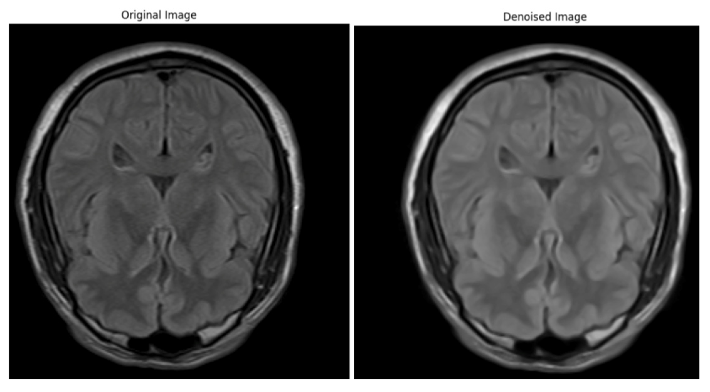
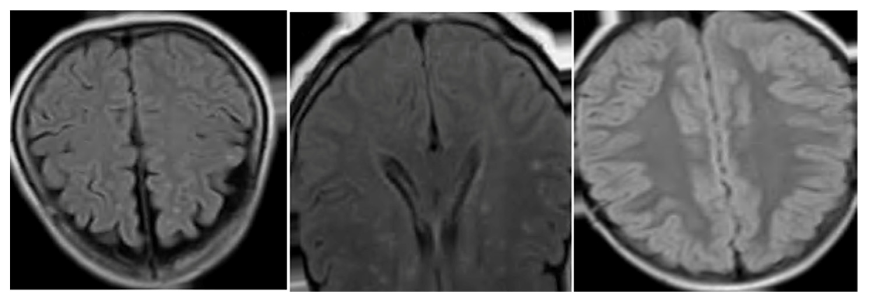
Artifacts and Noise Reduction
Bias Field Correction
Image Normalization
Resampling and Spacing Normalization
The UNet Preprocessing
- Loadimaged: means to load the *. nifty files.
- ToTensord: converts the transformed data into torch tensors so we can use them for training.
- Resized: allows the same dimensions for all patients.
- AddChanneld: allows us to add a channel to our image (volume) and label. This means adding channels in agreement with our class; in this case, 0, 1, and 2 for background, ischemia, and demyelination, respectively.
- Spacingd: Allows to change the voxel dimensions to have the same dimensions independently if the dataset of medical images was acquired with the same scan or with different scans, and consequently, they may have different voxel dimensions (width, height, and depth).
- ScalIntensityRanged: Allows the contrast change and normalizes the voxel values between 0 and 1. That is important because the training will be faster.
- CropForegroundd: Assists us in cropping out the empty regions of the image that we do not require, leaving only the region of interest.
3.1.3. Data Augmentation
Classical Data Augmentation
GAN Data Augmentation
3.2. Models
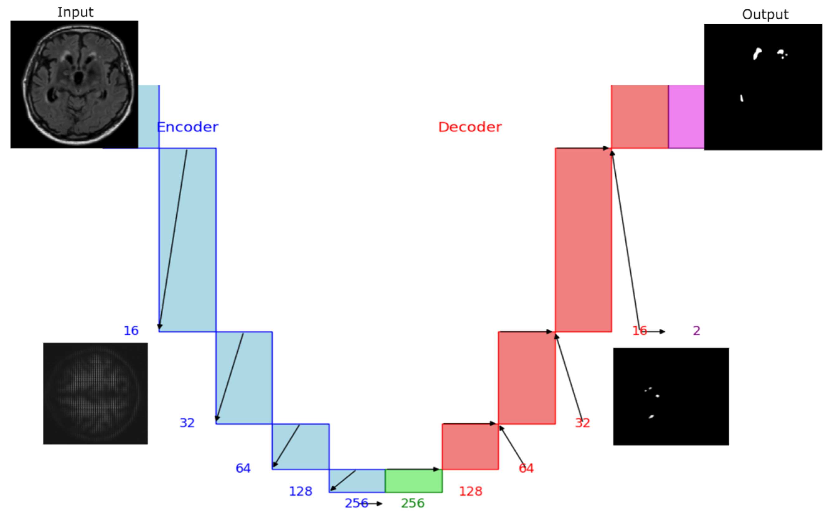
3.2.1. UNet Model
3.2.2. Segmenting Anything Model (SAM)
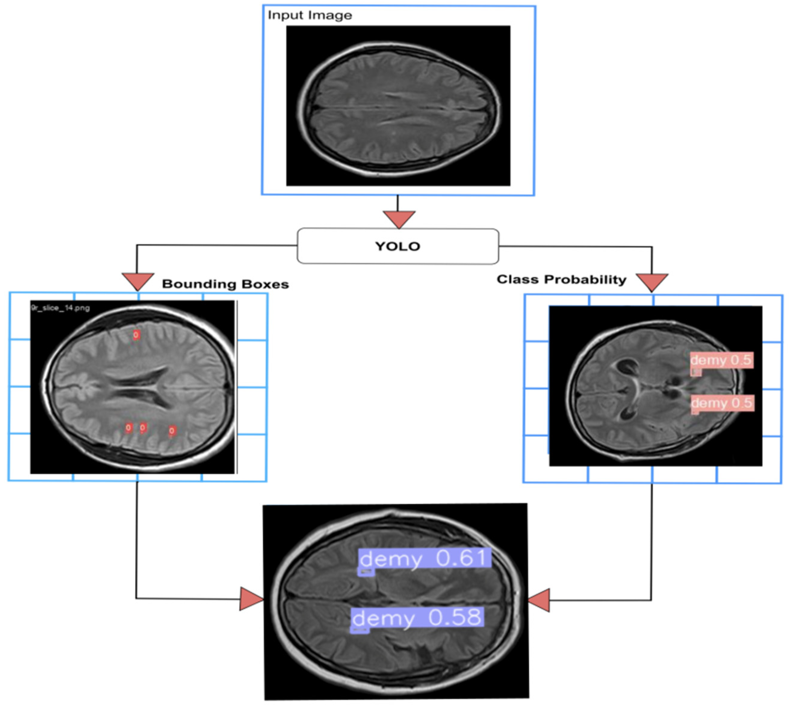
3.2.3. YOLO Model
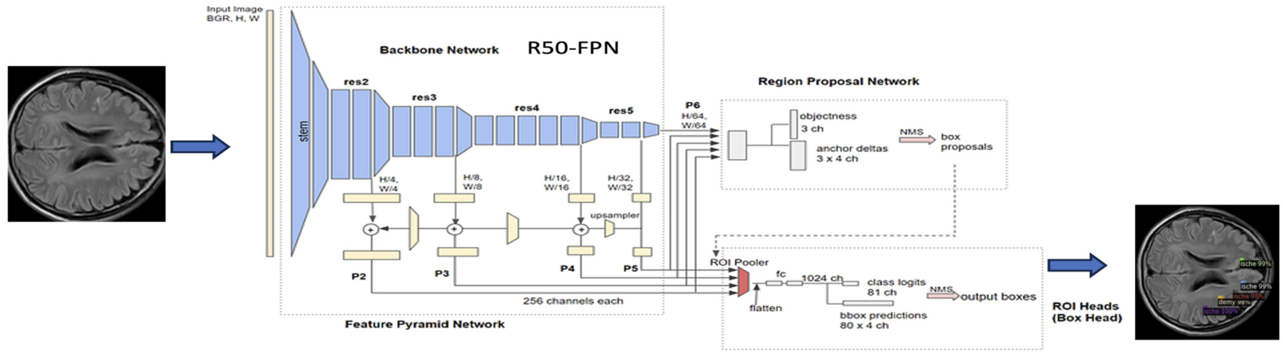
3.2.4. Detectron2 Model
3.3. Tools and Computational Resources
4. Results
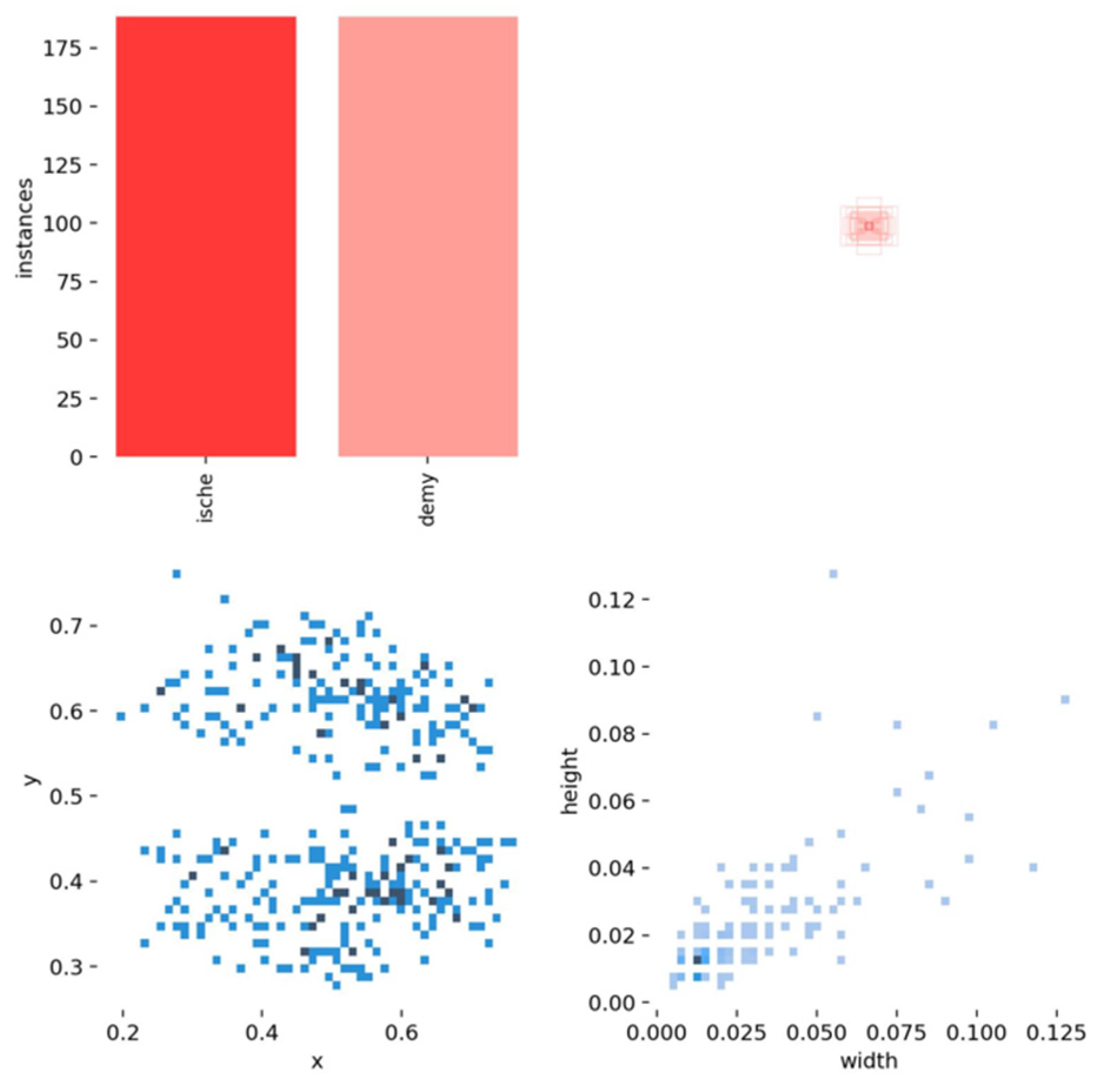
4.1. Label Analysis
- In section (a), the scatter plot in the (x, y) shows a correlation between the horizontal and vertical positions of the lesions in the brain, where they are more likely to occur in certain brain areas. The x and y histograms show the frequency of lesion positions. The distributions indicate that lesions are more frequently found in certain brain areas.
- In section (b), the scatter plots (x, width) and (y, width) show a more spread distribution with no strong pattern, indicating weak or no direct correlation between lesion positions and their width.
- In section (c), the scatter plot (width, height) suggests a more dispersed pattern, indicating that the width and height of lesions do not have a strong correlation. Lesions come in various shapes and sizes.
- The width and height histograms indicate that most lesions have small dimensions, between 0 and 0.4, and most cases have a size of less than 0.2 pixels. Fewer lesions have larger dimensions.
4.2. Segmentation Results
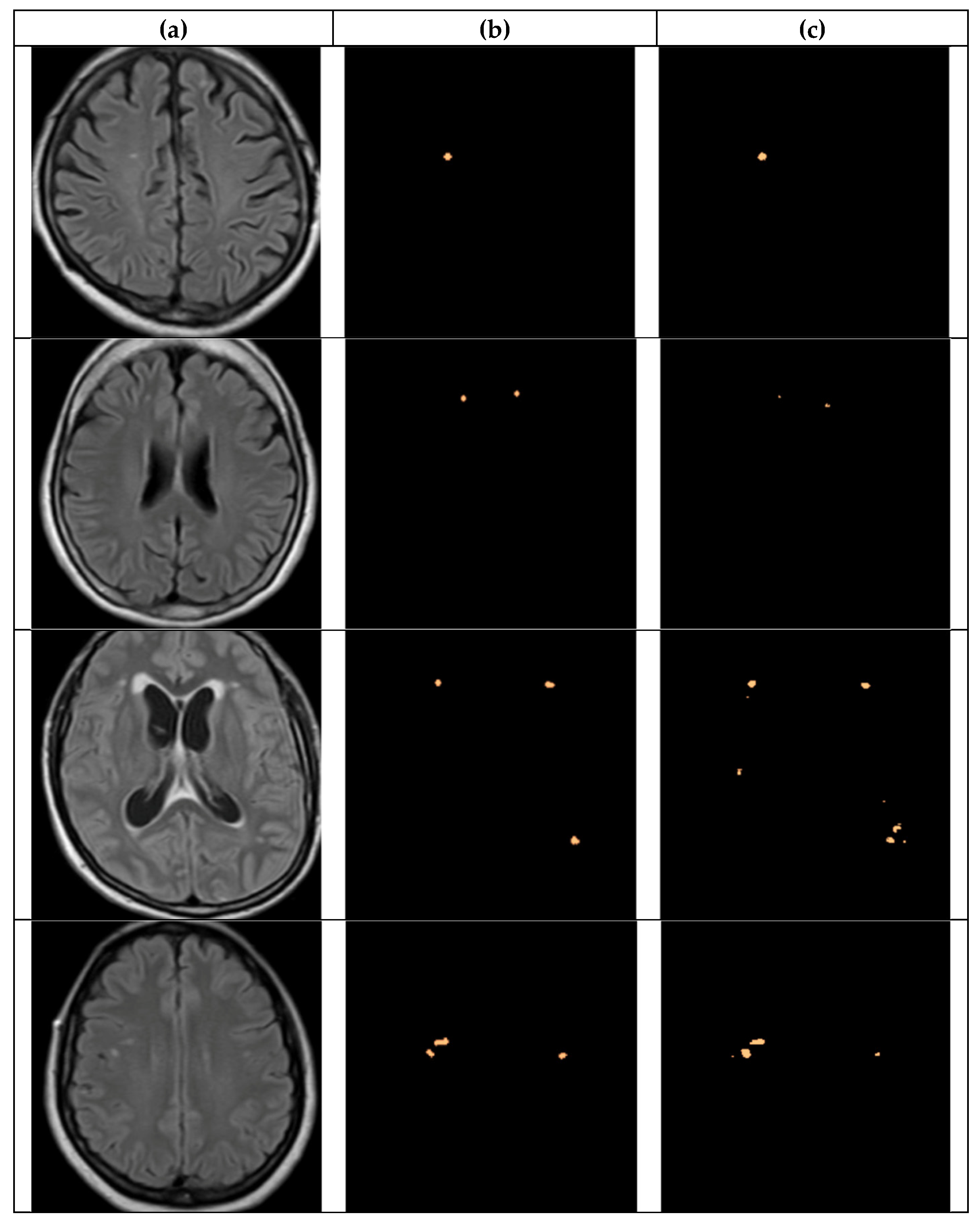
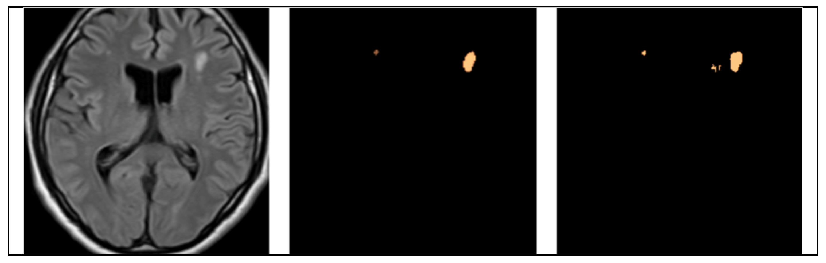
4.2.1. UNet Segmentation
4.2.2. SAM Model
- Effective initial learning: we can see in the three graphs a rapid initial drop in training loss: (~0.002) for vit-base, (~0.08) for vit-large but dropping sharply to stabilize around 0.002, and (~0.012) for vit-huge, which stabilizes quickly around 0.002. In general, this indicates effective learning from the start.
- Low and Stable Training Loss: Consistently low training loss across all graphs suggests a good model fit for the training data.
- Validation Loss Fluctuations: We can see there is variability in validation loss across all models, which suggests the challenges in the generalization that it is principally due to the limited training data. The most fluctuations between 0.004 and 0.006.
4.2.3. YOLO Model for Detecting WMH Lesions
- The curves of “train/box_loss” and “val/box_loss” show the training and validation loss related to the bounding box predictions. As the loss function decreases, it signifies that the network is effectively learning and enhancing its capability to precisely predict well-fitted bounding boxes.
- The “train/seg_loss” and “val/seg_loss” represents the training and validation segmentation loss.
- The “train/cls_loss” and “val/cls_loss” refer to training classification loss, which evaluates the classification accuracy of each predicted bounding box.
- The “train/dfl_loss” and “val/dfl_loss” indicate the training distribution focal loss, indicating the model’s confidence in predictions.
- The graph of “metrics/precision(B)” and “metrics/precision(M)” indicates the precision for bounding box predictions and precision for mask predictions, respectively.
- The “metrics/recall(B)” and “metrics/recall(M)” are the recall for bounding box predictions and recall for mask predictions, respectively. This indicates the ability to identify true positive masks.
- The “metrics/mAP50(B)” and “metrics/mAP50(M)” are the mean average precision at 50% IoU (Intersection over Union) for bounding boxes and for masks, respectively.
- The “metrics/mAP50-95(B)” and “metrics/mAP50-95(M)” are the mean average precision at IoU thresholds from 50% to 95% for bounding boxes and for masks, respectively.
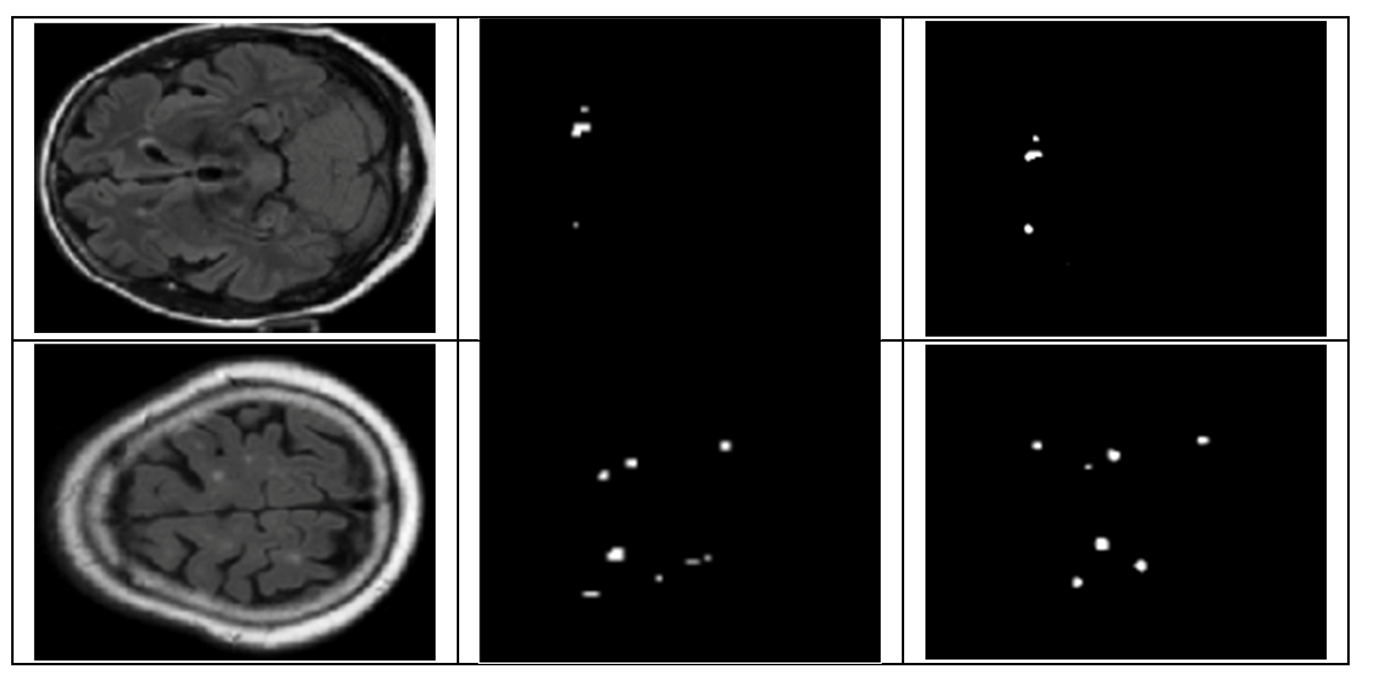
4.2.4. Detectron2 for Detecting WMH Lesions
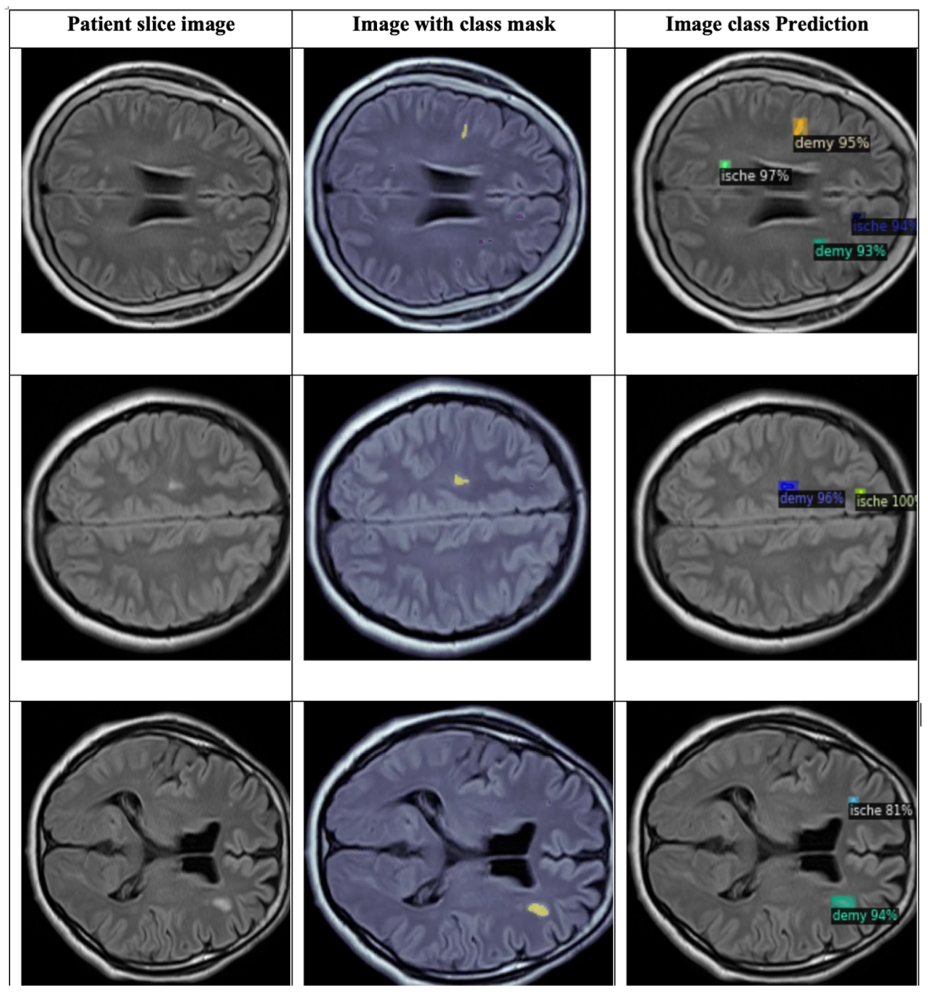
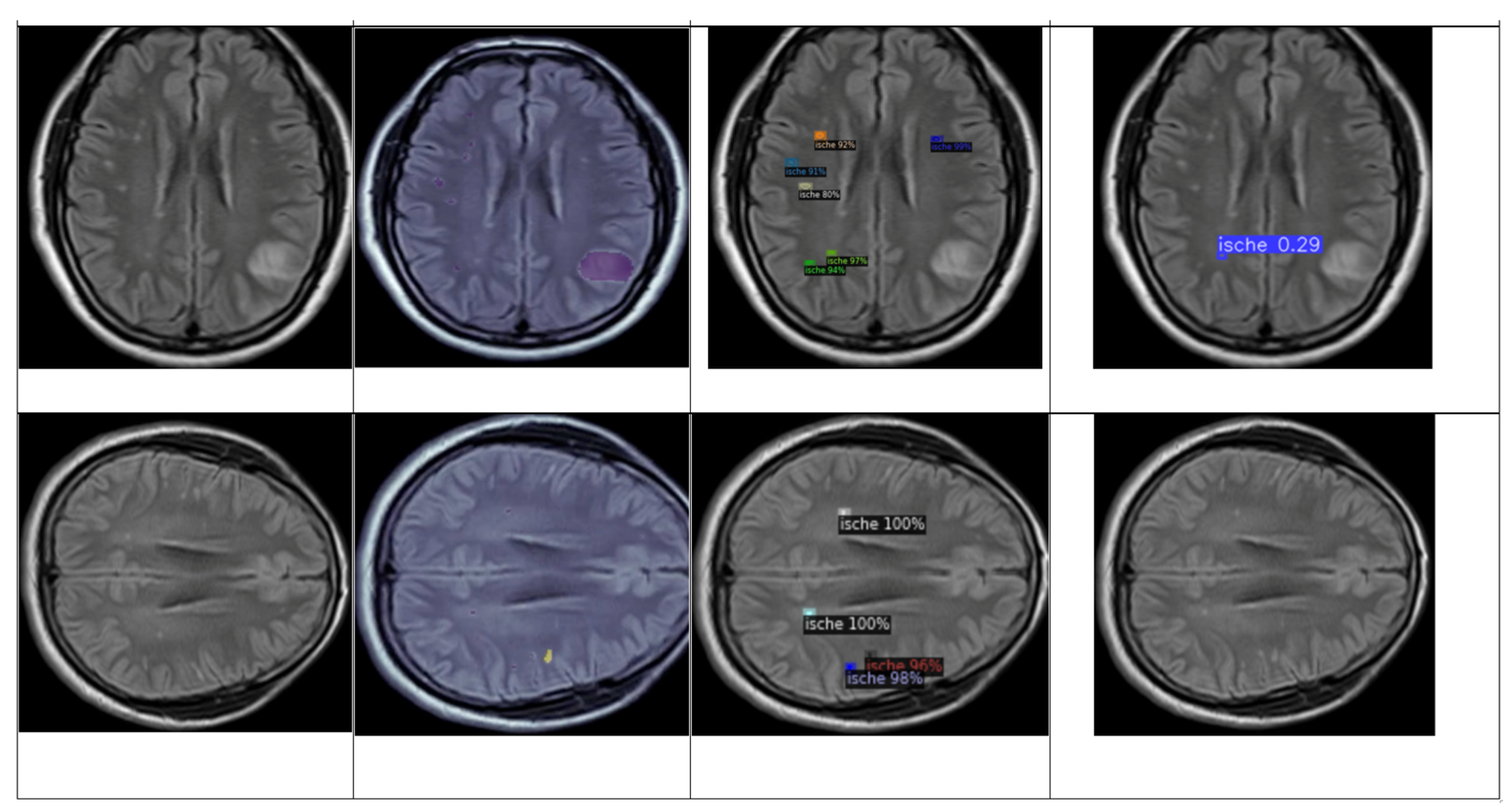
4.3. Detection and Classification
4.3.1. YOLOv8 Model for Detection and Classification
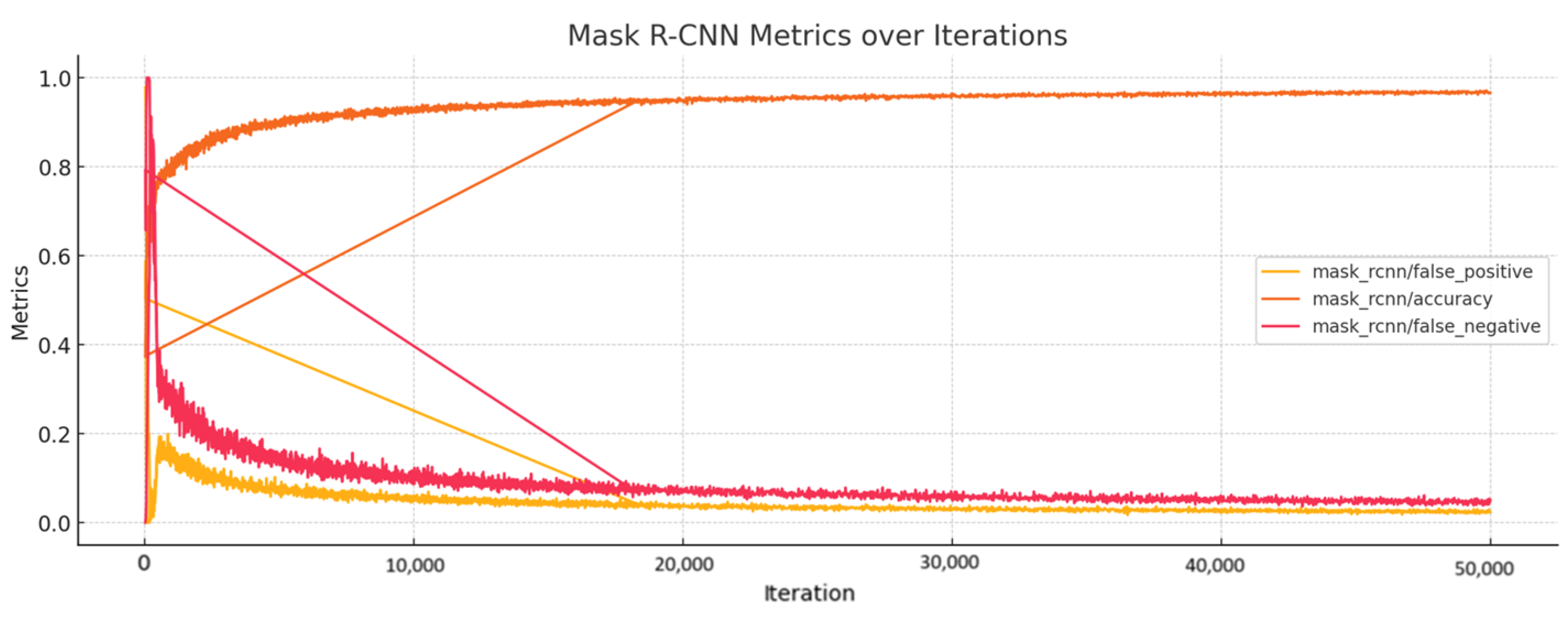
4.3.2. DETECTRON2 Model for Detection and Classification
- The total loss (‘total_loss’, mean value 0.300) indicates that the model has learned the essential features needed for classification and stabilization with minor fluctuations.
- The box regression loss (‘loss_box_reg’, mean value 0.072) decreases as the model learns to predict better-bounding boxes after stabilizing at a low value. This indicates that the model has become proficient in predicting bounding box coordinates.
- The classification loss (‘loss_cls’, mean value 0.030), through the pass of iteration, decreases and stabilizes, which suggests the model has learned to classify most of the lesions correctly.
- The mask loss (‘loss_mask’, mean value 0.154), shows decreasing and stabilizing values, which indicate a consistent performance in mask predictions.
- The RPN classification loss (‘loss_rpn_cls’, mean value 0.007) indicates a stabilization, which means that the region proposal classification task model has learned to propose regions accurately.
- The RPN localization loss (‘loss_rpn_loc’, mean value 0.029) stabilizes at a low value, which indicates the model’s proficiency with the localizing regions.
- The classification accuracy (‘fast_rcnn/cls_accuracy’ and ‘mask_rcnn/accuracy’) shows improvement through the iterations and gets stabilization values of 0.98 and 0.93 for both accuracies, respectively, which means the model is classifying lesions correctly most of the time (fast_rcnn/cls_accuracy) and that the model has high accuracy in mask prediction (mask_rcnn/accuracy).
4.4. Comparison of Proposed Segmentation Models
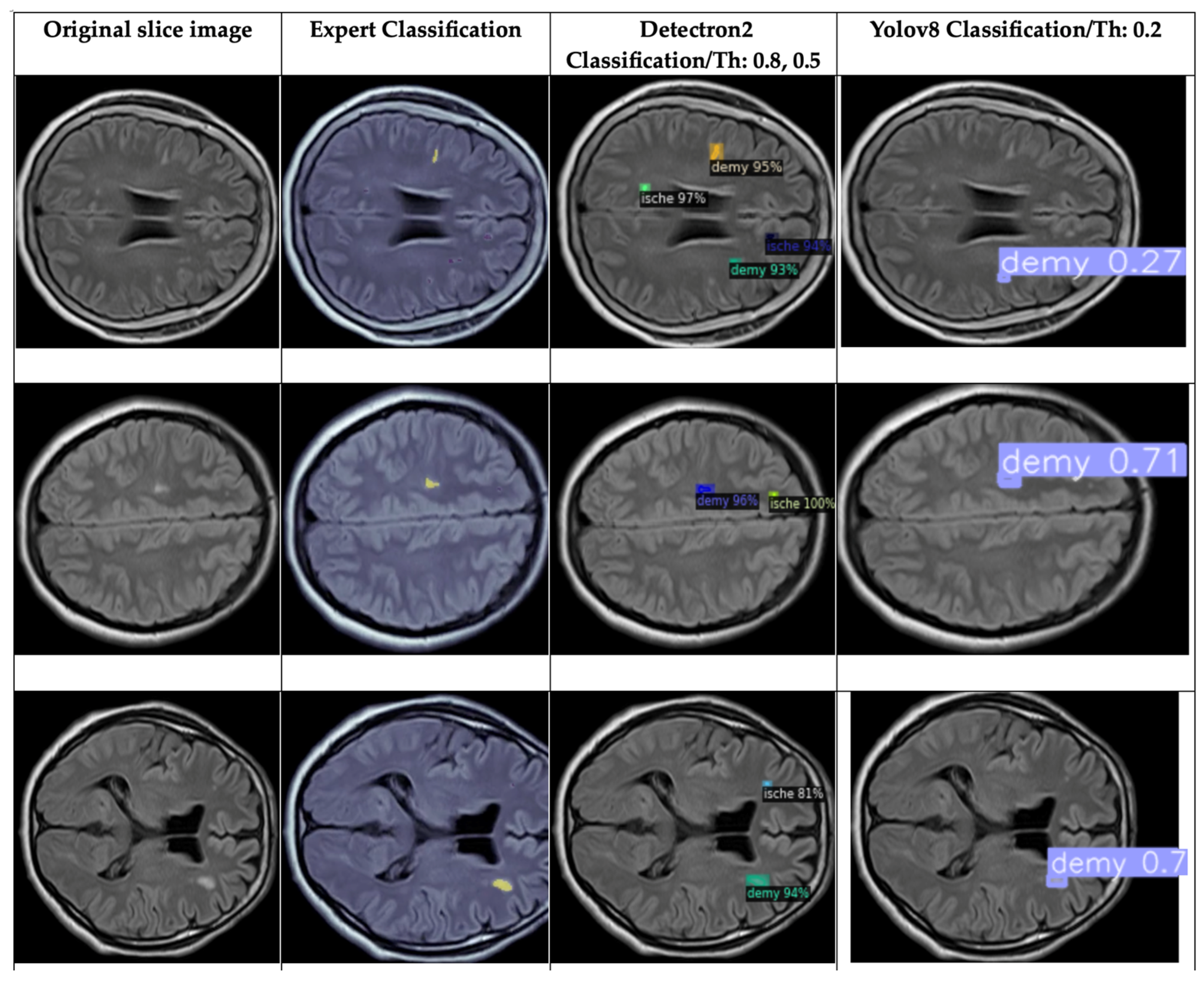
4.5. Brief Comparison Results Between Expert Criteria and YOLO and Detectron2 Models for Classification of Ischemia and Demyelination Lesions
5. Discussion
Limitations and Challenges
- The limited quantity of data concerning the specific pathologies of ischemia and demyelination diseases. To improve the segmentation and reduce the possible sources of noise that can affect the model, we only selected the range of slices of each volume with the lesions with their corresponding annotations. However, as with all deep learning methodologies, achieving optimal accuracy depends on the availability of large-scale datasets to ensure robust model performance and generalization.
- Although we used the public database provided by the MICCAI challenge, we cannot use the combined data to classify the lesions because the public data does not contain targets of the pathologies studied in this project. For that reason, the segmentation, detection, and identification of the WMH lesions were also made like a complementary project.
- The variability of the public data, in the sense that it was acquired from different equipment, may introduce bias, affecting model performance. Another limitation with respect to the data is that the private dataset is built with the annotation of experts by only one health institution; according to the literature, together with the artifacts and the noise produced with the equipment, the annotations also depend on the physician’s expertise.
- The detailed exploration of GANs will increase the dataset with synthetic images and build a more robust model of segmentation and classification of lesions. In this project, this idea was used; however, the synthetic images were not good enough for use in our dataset. Therefore, this is a motivational step to perform more research related to this theme in future works.
- The computational resources; running deep learning models based on 3D-based networks requires high-performance GPUs, which were not available for this study. Another limitation is that it was not possible to work with the 3D volume of the FLAIR MRI due principally to the characteristics of the specific images of our private dataset.
6. Conclusions
Future Works
Author Contributions
Funding
Institutional Review Board Statement
Informed Consent Statement
Data Availability Statement
Acknowledgments
Conflicts of Interest
Appendix A
- Code, Processors, and Time

| Model | Epochs/Iterations | Time Processing (s) | Processor |
|---|---|---|---|
| UNet | 250 | 90,389 | Google Colab Pro: Tesla V100-SXM2-16GB |
| SAM-Vit-Base | 25 50 | 189.6/epoch Total = 9480 | |
| SAM-Vit-Large | 25 50 | 189.6/epoch Total = 9480 | |
| SAM-Vit-Huge | 25 50 | 347.4/epoch Total = 17,370 | |
| YOLOv8 (private data) | 100 | 30–40/epoch Total = 4123 | |
| YOLOv8 (private+public data) | 100 | 180–190/epoch Total = 18,954 | |
| Detectron2 (private data) | 500k/iterations-250 epochs | 4909 | |
| Detectron2 (private+public data) | 500k/iterations-250 epochs | 5569 |
References
- World Health Organization. Neurological Disorders: Public Health Challenges; World Health Organization: Geneva, Switzerland, 2006. [Google Scholar]
- Marek, M.; Horyniecki, M.; Frączek, M.; Kluczewska, E. Leukoaraiosis—New Concepts and Modern Imaging. Pol. J. Radiol. 2018, 83, e76. [Google Scholar] [CrossRef] [PubMed]
- Merino, J.G. White Matter Hyperintensities on Magnetic Resonance Imaging: What Is a Clinician to Do? Mayo Clin. Proc. 2019, 94, 380–382. [Google Scholar] [CrossRef] [PubMed]
- White Matter Hyperintensities on MRI—Artefact or Something Sinister? Available online: https://psychscenehub.com/psychinsights/white-matter-hyperintensities-mri/ (accessed on 21 April 2022).
- Ammirati, E.; Moroni, F.; Magnoni, M.; Rocca, M.A.; Anzalone, N.; Cacciaguerra, L.; di Terlizzi, S.; Villa, C.; Sizzano, F.; Palini, A.; et al. Progression of Brain White Matter Hyperintensities in Asymptomatic Patients with Carotid Atherosclerotic Plaques and No Indication for Revascularization. Atherosclerosis 2019, 287, 171–178. [Google Scholar] [CrossRef] [PubMed]
- Ischemic Stroke: MedlinePlus. Available online: https://medlineplus.gov/ischemicstroke.html (accessed on 22 April 2022).
- Stroke|Mayfield Brain & Spine, Cincinnati, Ohio. Available online: https://mayfieldclinic.com/pe-stroke.htm (accessed on 22 April 2022).
- Types of Stroke | Johns Hopkins Medicine. Available online: https://www.hopkinsmedicine.org/health/conditions-and-diseases/stroke/types-of-stroke (accessed on 22 April 2022).
- Nour, M.; Liebeskind, D.S. Imaging of Cerebral Ischemia: From Acute Stroke to Chronic Disorders. Neurol. Clin. 2014, 32, 193–209. [Google Scholar] [CrossRef]
- Mehndiratta, M.M.; Gulati, N.S. Central and Peripheral Demyelination. J. Neurosci. Rural Pract. 2014, 5, 84–86. [Google Scholar] [CrossRef]
- Love, S. Demyelinating Diseases. J. Clin. Pathol. 2006, 59, 1151–1159. [Google Scholar] [CrossRef]
- Overview of Demyelinating Disorders—Brain, Spinal Cord, and Nerve Disorders—MSD Manual Consumer Version. Available online: https://www.msdmanuals.com/home/brain,-spinal-cord,-and-nerve-disorders/multiple-sclerosis-ms-and-related-disorders/overview-of-demyelinating-disorders (accessed on 26 April 2022).
- Leite, M.; Rittner, L.; Appenzeller, S.; Ruocco, H.H.; Lotufo, R. Etiology-Based Classification of Brain White Matter Hyperintensity on Magnetic Resonance Imaging. J. Med. Imaging 2015, 2, 014002. [Google Scholar] [CrossRef]
- Rachmadi, M.F.; Valdés-Hernández, M.d.C.; Makin, S.; Wardlaw, J.; Komura, T. Automatic Spatial Estimation of White Matter Hyperintensities Evolution in Brain MRI Using Disease Evolution Predictor Deep Neural Networks. Med. Image Anal. 2020, 63, 101712. [Google Scholar] [CrossRef]
- Diniz, P.H.B.; Valente, T.L.A.; Diniz, J.O.B.; Silva, A.C.; Gattass, M.; Ventura, N.; Muniz, B.C.; Gasparetto, E.L. Detection of White Matter Lesion Regions in MRI Using SLIC0 and Convolutional Neural Network. Comput. Methods Programs Biomed. 2018, 167, 49–63. [Google Scholar] [CrossRef]
- Park, G.; Hong, J.; Duffy, B.A.; Lee, J.M.; Kim, H. White Matter Hyperintensities Segmentation Using the Ensemble U-Net with Multi-Scale Highlighting Foregrounds. Neuroimage 2021, 237, 118140. [Google Scholar] [CrossRef]
- Eichinger, P.; Schön, S.; Pongratz, V.; Wiestler, H.; Zhang, H.; Bussas, M.; Hoshi, M.M.; Kirschke, J.; Berthele, A.; Zimmer, C.; et al. Accuracy of Unenhanced MRI in the Detection of New Brain Lesions in Multiple Sclerosis. Radiology 2019, 291, 429–435. [Google Scholar] [CrossRef] [PubMed]
- Rudie, J.D.; Mattay, R.R.; Schindler, M.; Steingall, S.; Cook, T.S.; Loevner, L.A.; Schnall, M.D.; Mamourian, A.C.; Bilello, M. An Initiative to Reduce Unnecessary Gadolinium-Based Contrast in Multiple Sclerosis Patients. J. Am. Coll. Radiol. 2019, 16, 1158–1164. [Google Scholar] [CrossRef] [PubMed]
- McKinley, R.; Wepfer, R.; Grunder, L.; Aschwanden, F.; Fischer, T.; Friedli, C.; Muri, R.; Rummel, C.; Verma, R.; Weisstanner, C.; et al. Automatic Detection of Lesion Load Change in Multiple Sclerosis Using Convolutional Neural Networks with Segmentation Confidence. Neuroimage Clin. 2020, 25, 102104. [Google Scholar] [CrossRef] [PubMed]
- Castillo, D.; Lakshminarayanan, V.; Rodríguez-Álvarez, M.J. MR Images, Brain Lesions, and Deep Learning. Appl. Sci. 2021, 11, 1675. [Google Scholar] [CrossRef]
- Li, Y.; Ammari, S.; Balleyguier, C.; Lassau, N.; Chouzenoux, E. Impact of Preprocessing and Harmonization Methods on the Removal of Scanner Effects in Brain MRI Radiomic Features. Cancers 2021, 13, 3000. [Google Scholar] [CrossRef]
- Kumar, A.; Upadhyay, N.; Ghosal, P.; Chowdhury, T.; Das, D.; Mukherjee, A.; Nandi, D. CSNet: A New DeepNet Framework for Ischemic Stroke Lesion Segmentation. Comput. Methods Programs Biomed. 2020, 193, 105524. [Google Scholar] [CrossRef]
- Hugo Lopez Pinaya, W.; Tudosiu, P.-D.; Gray, R.; Rees, G.; Nachev, P.; Ourselin, S.; Cardoso, M.J. Unsupervised Brain Anomaly Detection and Segmentation with Transformers. Proc. Mach. Learn. Res. 2021, 143, 596–617. [Google Scholar]
- Zhao, Z.; Alzubaidi, L.; Zhang, J.; Duan, Y.; Gu, Y. A Comparison Review of Transfer Learning and Self-Supervised Learning: Definitions, Applications, Advantages and Limitations. Expert Syst. Appl. 2024, 242, 122807. [Google Scholar] [CrossRef]
- Maier, O.; Schröder, C.; Forkert, N.D.; Martinetz, T.; Handels, H. Classifiers for Ischemic Stroke Lesion Segmentation: A Comparison Study. PLoS ONE 2015, 10, e0145118. [Google Scholar] [CrossRef]
- Weng, W.; Zhu, X. U-Net: Convolutional Networks for Biomedical Image Segmentation. IEEE Access 2015, 9, 16591–16603. [Google Scholar] [CrossRef]
- Kirillov, A.; Mintun, E.; Ravi, N.; Mao, H.; Rolland, C.; Gustafson, L.; Xiao, T.; Whitehead, S.; Berg, A.C.; Lo, W.Y.; et al. Segment Anything. In Proceedings of the IEEE International Conference on Computer Vision, Paris, France, 1–6 October 2023; pp. 3992–4003. [Google Scholar] [CrossRef]
- Ultralytics Home—Ultralytics YOLOv8 Docs. Available online: https://docs.ultralytics.com/ (accessed on 25 May 2024).
- Wu, Y.; Kirillov, A.; Massa, F.; Lo, W.-Y.; Girshick, R. Detectron2. Available online: https://github.com/facebookresearch/detectron2 (accessed on 17 July 2024).
- Hussain, S.; Anwar, S.M.; Majid, M. Segmentation of Glioma Tumors in Brain Using Deep Convolutional Neural Network. Neurocomputing 2018, 282, 248–261. [Google Scholar] [CrossRef]
- Nadeem, M.W.; al Ghamdi, M.A.; Hussain, M.; Khan, M.A.; Khan, K.M.; Almotiri, S.H.; Butt, S.A. Brain Tumor Analysis Empowered with Deep Learning: A Review, Taxonomy, and Future Challenges. Brain Sci. 2020, 10, 118. [Google Scholar] [CrossRef] [PubMed]
- Anwar, S.M.; Majid, M.; Qayyum, A.; Awais, M.; Alnowami, M.; Khan, M.K. Medical Image Analysis Using Convolutional Neural Networks: A Review. J. Med. Syst. 2018, 42, 226. [Google Scholar] [CrossRef] [PubMed]
- Ronneberger, O.; Fischer, P.; Brox, T. U-Net: {Convolutional} Networks for Biomedical Image Segmentation. In Proceedings of the Medical Image Computing and Computer-Assisted Intervention—MICCAI 2015, Munich, Germany, 5–9 October 2015; Lecture Notes in Computer Science (including subseries Lecture Notes in Artificial Intelligence and Lecture Notes in Bioinformatics). Volume 9351, pp. 234–241. [Google Scholar] [CrossRef]
- Clèrigues, A.; Valverde, S.; Bernal, J.; Freixenet, J.; Oliver, A.; Lladó, X. Acute and Sub-Acute Stroke Lesion Segmentation from Multimodal MRI. Comput. Methods Programs Biomed. 2020, 194, 105521. [Google Scholar] [CrossRef]
- Guerrero, R.; Qin, C.; Oktay, O.; Bowles, C.; Chen, L.; Joules, R.; Wolz, R.; Valdés-Hernández, M.C.; Dickie, D.A.; Wardlaw, J.; et al. White Matter Hyperintensity and Stroke Lesion Segmentation and Differentiation Using Convolutional Neural Networks. Neuroimage Clin. 2018, 17, 918–934. [Google Scholar] [CrossRef]
- Mitra, J.; Bourgeat, P.; Fripp, J.; Ghose, S.; Rose, S.; Salvado, O.; Connelly, A.; Campbell, B.; Palmer, S.; Sharma, G.; et al. Lesion Segmentation from Multimodal MRI Using Random Forest Following Ischemic Stroke. Neuroimage 2014, 98, 324–335. [Google Scholar] [CrossRef]
- Ghafoorian, M.; Karssemeijer, N.; van Uden, I.W.M.; de Leeuw, F.-E.; Heskes, T.; Marchiori, E.; Platel, B. Automated Detection of White Matter Hyperintensities of All Sizes in Cerebral Small Vessel Disease. Med. Phys. 2016, 43, 6246. [Google Scholar] [CrossRef]
- Liu, M.; Wang, T.; Liu, D.; Gao, F.; Cao, J. Improved UNet-Based Magnetic Resonance Imaging Segmentation of Demyelinating Diseases with Small Lesion Regions. Cogn. Comput. Syst. 2024, 1–8. [Google Scholar] [CrossRef]
- Zhou, D.; Xu, L.; Wang, T.; Wei, S.; Gao, F.; Lai, X.; Cao, J. M-DDC: MRI Based Demyelinative Diseases Classification with U-Net Segmentation and Convolutional Network. Neural Netw. 2024, 169, 108–119. [Google Scholar] [CrossRef]
- Ma, J.; He, Y.; Li, F.; Han, L.; You, C.; Wang, B. Segment Anything in Medical Images. Nat. Commun. 2024, 15, 654. [Google Scholar] [CrossRef] [PubMed]
- Hu, X.; Xu, X.; Shi, Y. How to Efficiently Adapt Large Segmentation Model(SAM) to Medical Images. arXiv 2023, arXiv:2306.13731. [Google Scholar]
- Tolstikhin, I.; Houlsby, N.; Kolesnikov, A.; Beyer, L.; Zhai, X.; Unterthiner, T.; Yung, J.; Steiner, A.; Keysers, D.; Uszkoreit, J.; et al. MLP-Mixer: An All-MLP Architecture for Vision. Adv. Neural Inf. Process. Syst. 2021, 29, 24261–24272. [Google Scholar]
- Dosovitskiy, A.; Beyer, L.; Kolesnikov, A.; Weissenborn, D.; Zhai, X.; Unterthiner, T.; Dehghani, M.; Minderer, M.; Heigold, G.; Gelly, S.; et al. An Image Is Worth 16x16 Words: Transformers For Image Recognition at Scale. arXiv 2020, arXiv:2010.11929. [Google Scholar]
- Mazurowski, M.A.; Dong, H.; Gu, H.; Yang, J.; Konz, N.; Zhang, Y. Segment Anything Model for Medical Image Analysis: An Experimental Study. Med. Image Anal. 2023, 89, 102918. [Google Scholar] [CrossRef]
- Huang, Y.; Yang, X.; Liu, L.; Zhou, H.; Chang, A.; Zhou, X.; Chen, R.; Yu, J.; Chen, J.; Chen, C.; et al. Segment Anything Model for Medical Images? Med. Image Anal. 2023, 92, 103061. [Google Scholar] [CrossRef]
- Cheng, D.; Qin, Z.; Jiang, Z.; Zhang, S.; Lao, Q.; Li, K. SAM on Medical Images: A Comprehensive Study on Three Prompt Modes. arXiv 2023, arXiv:2305.00035. [Google Scholar]
- Tu, Z.; Gu, L.; Wang, X.; Jiang, B.; Provincial, A. Ultrasound SAM Adapter: Adapting SAM for Breast Lesion Segmentation in Ultrasound Images. arXiv 2024, arXiv:2404.14837. [Google Scholar]
- Bhardwaj, R.B.; Haneef, D.A. Use of Segment Anything Model (SAM) and MedSAM in the Optic Disc Segmentation of Colour Retinal Fundus Images: Experimental Finding. Indian J. Health Care Med. Pharm. Pract. 2023, 4, 82–93. [Google Scholar] [CrossRef]
- Fazekas, B.; Morano, J.; Lachinov, D.; Aresta, G.; Bogunović, H. Adapting Segment Anything Model (SAM) for Retinal OCT. In Proceedings of the OMIA 2023, Vancouver, BC, Canada, 12 October 2023; Lecture Notes in Computer Science (including subseries Lecture Notes in Artificial Intelligence and Lecture Notes in Bioinformatics). Volume 14096 LNCS, pp. 92–101. [Google Scholar] [CrossRef]
- Zhao, Y.; Song, K.; Cui, W.; Ren, H.; Yan, Y. MFS Enhanced SAM: Achieving Superior Performance in Bimodal Few-Shot Segmentation. J. Vis. Commun. Image Represent. 2023, 97, 103946. [Google Scholar] [CrossRef]
- Li, N.; Xiong, L.; Qiu, W.; Pan, Y.; Luo, Y.; Zhang, Y. Segment Anything Model for Semi-Supervised Medical Image Segmentation via Selecting Reliable Pseudo-Labels. Commun. Comput. Inf. Sci. 2024, 1964 CCIS, 138–149. [Google Scholar] [CrossRef]
- Ravishankar, H.; Patil, R.; Melapudi, V.; Annangi, P. SonoSAM—Segment Anything on Ultrasound Images. In Proceedings of the ASMUS 2023, Vancouver, BC, Canada, 8 October 2023; Lecture Notes in Computer Science (including subseries Lecture Notes in Artificial Intelligence and Lecture Notes in Bioinformatics). Volume 14337 LNCS, pp. 23–33. [Google Scholar] [CrossRef]
- Jiménez-Gaona, Y.; Álvarez, M.J.R.; Castillo-Malla, D.; García-Jaen, S.; Carrión-Figueroa, D.; Corral-Domínguez, P.; Lakshminarayanan, V. BraNet: A Mobil Application for Breast Image Classification Based on Deep Learning Algorithms. Med. Biol. Eng. Comput. 2024, 62, 2737–2756. [Google Scholar] [CrossRef] [PubMed]
- Zhang, Y.; Shen, Z.; Jiao, R. Segment Anything Model for Medical Image Segmentation: Current Applications and Future Directions. Comput. Biol. Med. 2024, 171, 108238. [Google Scholar] [CrossRef] [PubMed]
- GitHub—YichiZhang98/SAM4MIS: Segment Anything Model for Medical Image Segmentation: Paper List and Open-Source Project Summary. Available online: https://github.com/YichiZhang98/SAM4MIS (accessed on 24 May 2024).
- Redmon, J.; Divvala, S.; Girshick, R.; Farhadi, A. You Only Look Once: Unified, Real-Time Object Detection. In Proceedings of the IEEE Computer Society Conference on Computer Vision and Pattern Recognition, Las Vegas, NV, USA, 27–30 June 2016; pp. 779–788. [Google Scholar] [CrossRef]
- Almufareh, M.F.; Imran, M.; Khan, A.; Humayun, M.; Asim, M. Automated Brain Tumor Segmentation and Classification in MRI Using YOLO-Based Deep Learning. IEEE Access 2024, 12, 16189–16207. [Google Scholar] [CrossRef]
- Mortada, M.J.; Tomassini, S.; Anbar, H.; Morettini, M.; Burattini, L.; Sbrollini, A. Segmentation of Anatomical Structures of the Left Heart from Echocardiographic Images Using Deep Learning. Diagnostics 2023, 13, 1683. [Google Scholar] [CrossRef]
- Ragab, M.G.; Abdulkader, S.J.; Muneer, A.; Alqushaibi, A.; Sumiea, E.H.; Qureshi, R.; Al-Selwi, S.M.; Alhussian, H. A Comprehensive Systematic Review of YOLO for Medical Object Detection (2018 to 2023). IEEE Access 2024, 12, 57815–57836. [Google Scholar] [CrossRef]
- Aldughayfiq, B.; Ashfaq, F.; Jhanjhi, N.Z.; Humayun, M. YOLO-Based Deep Learning Model for Pressure Ulcer Detection and Classification. Healthcare 2023, 11, 1222. [Google Scholar] [CrossRef]
- Chen, J.L.; Cheng, L.H.; Wang, J.; Hsu, T.W.; Chen, C.Y.; Tseng, L.M.; Guo, S.M. A YOLO-Based AI System for Classifying Calcifications on Spot Magnification Mammograms. Biomed. Eng. Online 2023, 22, 54. [Google Scholar] [CrossRef]
- Baccouche, A.; Garcia-Zapirain, B.; Olea, C.C.; Elmaghraby, A.S. Breast Lesions Detection and Classification via YOLO-Based Fusion Models. Comput. Mater. Contin. 2021, 69, 1407–1425. [Google Scholar] [CrossRef]
- Santos, C.; Aguiar, M.; Welfer, D.; Belloni, B. A New Approach for Detecting Fundus Lesions Using Image Processing and Deep Neural Network Architecture Based on YOLO Model. Sensors 2022, 22, 6441. [Google Scholar] [CrossRef]
- Ünver, H.M.; Ayan, E. Skin Lesion Segmentation in Dermoscopic Images with Combination of YOLO and GrabCut Algorithm. Diagnostics 2019, 9, 72. [Google Scholar] [CrossRef]
- Kang, M.; Ting, C.-M.; Ting, F.F.; Phan, R.C.-W. ASF-YOLO: A Novel YOLO Model with Attentional Scale Sequence Fusion for Cell Instance Segmentation. Image Vis. Comput. 2024, 147, 105057. [Google Scholar] [CrossRef]
- Abdusalomov, A.B.; Mukhiddinov, M.; Whangbo, T.K. Brain Tumor Detection Based on Deep Learning Approaches and Magnetic Resonance Imaging. Cancers 2023, 15, 4172. [Google Scholar] [CrossRef] [PubMed]
- Mercaldo, F.; Brunese, L.; Martinelli, F.; Santone, A.; Cesarelli, M. Object Detection for Brain Cancer Detection and Localization. Appl. Sci. 2023, 13, 9158. [Google Scholar] [CrossRef]
- He, K.; Gkioxari, G.; Dollár, P.; Girshick, R. Mask R-CNN. IEEE Trans. Pattern Anal. Mach. Intell. 2017, 42, 386–397. [Google Scholar] [CrossRef]
- Girshick, R. Fast R-CNN. In Proceedings of the 2015 IEEE International IEEE Conference on Computer Vision (ICCV), Santiago, Chile, 7–13 December 2015; pp. 1440–1448. [Google Scholar]
- Zhang, H.; Chang, H.; Ma, B.; Shan, S.; Chen: Cascade, X.; Zhang, H.; Chang, H.; Cn Bingpeng Ma, A.; Shan, S.; Chen, X. Cascade RetinaNet: Maintaining Consistency for Single-Stage Object Detection. In Proceedings of the 30th British Machine Vision Conference 2019, BMVC 2019, Cardiff, UK, 9–12 September 2019. [Google Scholar]
- Detectron2: A PyTorch-Based Modular Object Detection Library. Available online: https://ai.meta.com/blog/-detectron2-a-pytorch-based-modular-object-detection-library-/ (accessed on 25 May 2024).
- Chincholi, F.; Koestler, H. Detectron2 for Lesion Detection in Diabetic Retinopathy. Algorithms 2023, 16, 147. [Google Scholar] [CrossRef]
- Salh, C.H.; Ali, A.M. Automatic Detection of Breast Cancer for Mastectomy Based on MRI Images Using Mask R-CNN and Detectron2 Models. Neural Comput. Appl. 2024, 36, 3017–3035. [Google Scholar] [CrossRef]
- Dipu, N.M.; Shohan, S.A.; Salam, K.M.A. Brain Tumor Detection Using Various Deep Learning Algorithms. In Proceedings of the 2021 International Conference on Science and Contemporary Technologies, ICSCT 2021, Dhaka, Bangladesh, 5–7 August 2021. [Google Scholar] [CrossRef]
- Home—WMH Segmentation Challenge. Available online: https://wmh.isi.uu.nl/ (accessed on 30 June 2022).
- Bologna, M.; Corino, V.; Mainardi, L. Technical Note: Virtual Phantom Analyses for Preprocessing Evaluation and Detection of a Robust Feature Set for MRI-Radiomics of the Brain. Med. Phys. 2019, 46, 5116–5123. [Google Scholar] [CrossRef]
- Masoudi, S.; Harmon, S.A.; Mehralivand, S.; Walker, S.M.; Raviprakash, H.; Bagci, U.; Choyke, P.L.; Turkbey, B. Quick Guide on Radiology Image Pre-Processing for Deep Learning Applications in Prostate Cancer Research. J. Med. Imaging 2021, 8, 010901. [Google Scholar] [CrossRef]
- Um, H.; Tixier, F.; Bermudez, D.; Deasy, J.O.; Young, R.J.; Veeraraghavan, H. Impact of Image Preprocessing on the Scanner Dependence of Multi-Parametric MRI Radiomic Features and Covariate Shift in Multi-Institutional Glioblastoma Datasets. Phys. Med. Biol. 2019, 64, 165011. [Google Scholar] [CrossRef]
- Orlhac, F.; Lecler, A.; Savatovski, J.; Goya-Outi, J.; Nioche, C.; Charbonneau, F.; Ayache, N.; Frouin, F.; Duron, L.; Buvat, I. How Can We Combat Multicenter Variability in MR Radiomics? Validation of a Correction Procedure. Eur. Radiol. 2021, 31, 2272–2280. [Google Scholar] [CrossRef]
- Zhang, K.; Song, H.; Zhang, L. Active Contours Driven by Local Image Fitting Energy. Pattern Recognit. 2010, 43, 1199–1206. [Google Scholar] [CrossRef]
- Tustison, N.J.; Avants, B.B.; Cook, P.A.; Zheng, Y.; Egan, A.; Yushkevich, P.A.; Gee, J.C. N4ITK: Improved N3 Bias Correction. IEEE Trans. Med. Imaging 2010, 29, 1310–1320. [Google Scholar] [CrossRef] [PubMed]
- Avants, B.B.; Tustison, N.J.; Wu, J.; Cook, P.A.; Gee, J.C. An Open Source Multivariate Framework for N-Tissue Segmentation with Evaluation on Public Data. Neuroinformatics 2011, 9, 381–400. [Google Scholar] [CrossRef] [PubMed]
- Shah, M.; Xiao, Y.; Subbanna, N.; Francis, S.; Arnold, D.L.; Collins, D.L.; Arbel, T. Evaluating Intensity Normalization on MRIs of Human Brain with Multiple Sclerosis. Med. Image Anal. 2011, 15, 267–282. [Google Scholar] [CrossRef]
- Consortium, M. MONAI: Medical Open Network for AI, Version 0.8.0; Zenodo: Genève, Switzerland, 2021. [CrossRef]
- MONAIBootcamp2021/1. Getting Started with MONAI.Ipynb at Main Project-MONAI/MONAIBootcamp2021 GitHub. Available online: https://github.com/Project-MONAI/MONAIBootcamp2021/blob/main/day1/1.%20Getting%20Started%20with%20MONAI.ipynb (accessed on 11 October 2022).
- Gupta, V.; Veeturi, N.; Akkur, A. Brain Aneurysm Classification from MRI Images Using MONAI Framework. CS230, Stanford University. Available online: http://cs230.stanford.edu/projects_winter_2021/reports/70747002.pdf (accessed on 20 January 2025).
- Diaz-Pinto, A.; Alle, S.; Ihsani, A.; Asad, M.; Nath, V.; Pérez-García, F.; Mehta, P.; Li, W.; Roth, H.R.; Vercauteren, T.; et al. MONAI Label: A Framework for AI-Assisted Interactive Labeling of 3D Medical Images. Med. Image Anal. 2024, 95, 103207. [Google Scholar] [CrossRef]
- MONAI—Home. Available online: https://monai.io/ (accessed on 4 October 2022).
- LeCun, Y.; Bengio, Y.; Hinton, G.; Goodfellow, I.; Bengio, Y.; Courville, A.; LeCun, Y.; Bengio, Y.; Hinton, G. Deep Learning. Nature 2015, 521, 436–444. [Google Scholar] [CrossRef]
- Goodfellow, I.; Pouget-Abadie, J.; Mirza, M.; Xu, B.; Warde-Farley, D.; Ozair, S.; Courville, A.; Bengio, Y. Generative Adversarial Nets. Adv. Neural Inf. Process. Syst. 2014, 27, 2672–2680. [Google Scholar]
- Jung, E.; Luna, M.; Park, S.H. Conditional GAN with 3D Discriminator for MRI Generation of Alzheimer’s Disease Progression. Pattern Recognit. 2023, 133, 109061. [Google Scholar] [CrossRef]
- Alrashedy, H.H.N.; Almansour, A.F.; Ibrahim, D.M.; Hammoudeh, M.A.A. BrainGAN: Brain MRI Image Generation and Classification Framework Using GAN Architectures and CNN Models. Sensors 2022, 22, 4297. [Google Scholar] [CrossRef]
- Woldesellasse, H.; Tesfamariam, S. Data Augmentation Using Conditional Generative Adversarial Network (CGAN): Application for Prediction of Corrosion Pit Depth and Testing Using Neural Network. J. Pipeline Sci. Eng. 2023, 3, 100091. [Google Scholar] [CrossRef]
- Shao, S.; Wang, P.; Yan, R. Generative Adversarial Networks for Data Augmentation in Machine Fault Diagnosis. Comput. Ind. 2019, 106, 85–93. [Google Scholar] [CrossRef]
- Borji, A. Pros and Cons of GAN Evaluation Measures. Comput. Vis. Image Underst. 2019, 179, 41–65. [Google Scholar] [CrossRef]
- Parmar, G.; Zhang, R.; Zhu, J.Y. On Aliased Resizing and Surprising Subtleties in GAN Evaluation. In Proceedings of the IEEE Computer Society Conference on Computer Vision and Pattern Recognition, New Orleans, LA, USA, 18–24 June 2022; pp. 11400–11410. [Google Scholar] [CrossRef]
- Detectron2/Configs/COCO-Detection/Faster_rcnn_R_50_FPN_3x.Yaml at Main Facebookresearch/Detectron2 GitHub. Available online: https://github.com/facebookresearch/detectron2/blob/main/configs/COCO-Detection/faster_rcnn_R_50_FPN_3x.yaml (accessed on 25 May 2024).
- Detectron2/Configs/COCO-InstanceSegmentation/Mask_rcnn_R_50_FPN_3x.Yaml at Main Facebookresearch/Detectron2 GitHub. Available online: https://github.com/facebookresearch/detectron2/blob/main/configs/COCO-InstanceSegmentation/mask_rcnn_R_50_FPN_3x.yaml (accessed on 25 May 2024).
- Ren, S.; He, K.; Girshick, R.; Sun, J. Faster R-CNN: Towards Real-Time Object Detection with Region Proposal Networks. IEEE Trans. Pattern Anal. Mach. Intell. 2017, 39, 1137–1149. [Google Scholar] [CrossRef] [PubMed]
- Li, X.; Zhao, Y.; Jiang, J.; Cheng, J.; Zhu, W.; Wu, Z.; Jing, J.; Zhang, Z.; Wen, W.; Sachdev, P.S.; et al. White Matter Hyperintensities Segmentation Using an Ensemble of Neural Networks. Hum. Brain Mapp. 2022, 43, 929–939. [Google Scholar] [CrossRef]
- Sahayam, S.; Abirami, A.; Jayaraman, U. A Novel Modified U-Shaped 3-D Capsule Network (MUDCap3) for Stroke Lesion Segmentation from Brain MRI. In Proceedings of the 4th IEEE Conference on Information and Communication Technology, CICT 2020, Chennai, India, 3–5 December 2020. [Google Scholar] [CrossRef]
- Zhang, H.; Zhu, C.; Lian, X.; Hua, F. A Nested Attention Guided UNet++ Architecture for White Matter Hyperintensity Segmentation. IEEE Access 2023, 11, 66910–66920. [Google Scholar] [CrossRef]
- Farkhani, S.; Demnitz, N.; Boraxbekk, C.J.; Lundell, H.; Siebner, H.R.; Petersen, E.T.; Madsen, K.H. End-to-End Volumetric Segmentation of White Matter Hyperintensities Using Deep Learning. Comput. Methods Programs Biomed. 2024, 245, 108008. [Google Scholar] [CrossRef]
- Li, H.; Jiang, G.; Zhang, J.; Wang, R.; Wang, Z.; Zheng, W.-S.; Menze, B. Fully Convolutional Network Ensembles for White Matter Hyperintensities Segmentation in MR Images. Neuroimage 2018, 183, 650–665. [Google Scholar] [CrossRef]
- Wu, J.; Zhang, Y.; Wang, K.; Tang, X. Skip Connection U-Net for White Matter Hyperintensities Segmentation from MRI. IEEE Access 2019, 7, 155194–155202. [Google Scholar] [CrossRef]
- Liu, L.; Chen, S.; Zhu, X.; Zhao, X.M.; Wu, F.X.; Wang, J. Deep Convolutional Neural Network for Accurate Segmentation and Quantification of White Matter Hyperintensities. Neurocomputing 2020, 384, 231–242. [Google Scholar] [CrossRef]
- Rathore, S.; Niazi, T.; Iftikhar, M.A.; Singh, A.; Rathore, B.; Bilello, M.; Chaddad, A. Multimodal Ensemble-Based Segmentation of White Matter Lesions and Analysis of Their Differential Characteristics across Major Brain Regions. Appl. Sci. 2020, 10, 1903. [Google Scholar] [CrossRef]
- Lee, A.R.; Woo, I.; Kang, D.W.; Jung, S.C.; Lee, H.; Kim, N. Fully Automated Segmentation on Brain Ischemic and White Matter Hyperintensities Lesions Using Semantic Segmentation Networks with Squeeze-and-Excitation Blocks in MRI. Inform Med. Unlocked 2020, 21, 100440. [Google Scholar] [CrossRef]
- Zhou, P.; Liang, L.; Guo, X.; Lv, H.; Wang, T.; Ma, T. U-Net Combined with CRF and Anatomical Based Spatial Features to Segment White Matter Hyperintensities. In Proceedings of the 2020 42nd Annual International Conference of the IEEE Engineering in Medicine & Biology Society (EMBC), Montreal, QC, Canada, 20–24 July 2020; pp. 1754–1757. [Google Scholar] [CrossRef]
- Karthik, R.; Menaka, R.; Hariharan, M.; Won, D. Ischemic Lesion Segmentation Using Ensemble of Multi-Scale Region Aligned CNN. Comput. Methods Programs Biomed. 2021, 200, 105831. [Google Scholar] [CrossRef] [PubMed]
- Zhang, S.; Xu, S.; Tan, L.; Wang, H.; Meng, J. Stroke Lesion Detection and Analysis in MRI Images Based on Deep Learning. J. Healthc. Eng. 2021, 2021, 5524769. [Google Scholar] [CrossRef]
- Uçar, G.; Dandil, E. Automatic Detection of White Matter Hyperintensities via Mask Region-Based Convolutional Neural Networks Using Magnetic Resonance Images. In Deep Learning for Medical Applications with Unique Data; Academic Press: Cambridge, MA, USA, 2022; pp. 153–179. [Google Scholar] [CrossRef]
- Chen, S.; Sedghi Gamechi, Z.; Dubost, F.; van Tulder, G.; de Bruijne, M. An End-to-End Approach to Segmentation in Medical Images with CNN and Posterior-CRF. Med. Image Anal. 2022, 76, 102311. [Google Scholar] [CrossRef]
- Wang, J.; Wang, S.; Liang, W. METrans: Multi-Encoder Transformer for Ischemic Stroke Segmentation. Electron. Lett. 2022, 58, 340–342. [Google Scholar] [CrossRef]
- Khezrpour, S.; Seyedarabi, H.; Razavi, S.N.; Farhoudi, M. Automatic Segmentation of the Brain Stroke Lesions from MR Flair Scans Using Improved U-Net Framework. Biomed. Signal Process. Control 2022, 78, 103978. [Google Scholar] [CrossRef]
- Uçar, G.; Dandıl, E. Enhanced Detection of White Matter Hyperintensities via Deep Learning-Enabled MR Imaging Segmentation. Trait. Du Signal 2024, 41, 1–21. [Google Scholar] [CrossRef]
- Soleimani, P.; Farezi, N. Utilizing Deep Learning via the 3D U-Net Neural Network for the Delineation of Brain Stroke Lesions in MRI Image. Sci. Rep. 2023, 13, 19808. [Google Scholar] [CrossRef]
- Liew, S.-L.; Anglin, J.M.; Banks, N.W.; Sondag, M.; Ito, K.L.; Kim, H.; Chan, J.; Ito, J.; Jung, C.; Khoshab, N.; et al. A Large, Open Source Dataset of Stroke Anatomical Brain Images and Manual Lesion Segmentations. Sci. Data 2018, 5, 180011. [Google Scholar] [CrossRef]
- Rieu, Z.H.; Kim, J.Y.; Kim, R.E.Y.; Lee, M.; Lee, M.K.; Oh, S.W.; Wang, S.M.; Kim, N.Y.; Kang, D.W.; Lim, H.K.; et al. Semi-Supervised Learning in Medical MRI Segmentation: Brain Tissue with White Matter Hyperintensity Segmentation Using Flair MRI. Brain Sci. 2021, 11, 720. [Google Scholar] [CrossRef]
- Rekik, I.; Allassonnière, S.; Carpenter, T.K.; Wardlaw, J.M. Medical Image Analysis Methods in MR/CT-Imaged Acute-Subacute Ischemic Stroke Lesion: Segmentation, Prediction and Insights into Dynamic Evolution Simulation Models. A Critical Appraisal. NeuroImage Clin. 2012, 1, 164–178. [Google Scholar] [CrossRef] [PubMed]
- Kuijf, H.J.; Biesbroek, J.M.; De Bresser, J.; Heinen, R.; Andermatt, S.; Bento, M.; Berseth, M.; Belyaev, M.; Cardoso, M.J.; Casamitjana, A.; et al. Standardized Assessment of Automatic Segmentation of White Matter Hyperintensities and Results of the WMH Segmentation Challenge. IEEE Trans. Med. Imaging 2019, 38, 2556–2568. [Google Scholar] [CrossRef] [PubMed]
- Weeda, M.M.; Brouwer, I.; de Vos, M.L.; de Vries, M.S.; Barkhof, F.; Pouwels, P.J.W.; Vrenken, H. Comparing Lesion Segmentation Methods in Multiple Sclerosis: {Input} from One Manually Delineated Subject Is Sufficient for Accurate Lesion Segmentation. Neuroimage Clin. 2019, 24, 102074. [Google Scholar] [CrossRef] [PubMed]
- Praveen, G.B.; Agrawal, A.; Sundaram, P.; Sardesai, S. Ischemic Stroke Lesion Segmentation Using Stacked Sparse Autoencoder. Comput. Biol. Med. 2018, 99, 38–52. [Google Scholar] [CrossRef]
- Khademi, A.; Gibicar, A.; Arezza, G.; DiGregorio, J.; Tyrrell, P.N.; Moody, A.R. Segmentation of White Matter Lesions in Multicentre FLAIR MRI. Neuroimage Rep. 2021, 1, 100044. [Google Scholar] [CrossRef]
- Mortazavi, D.; Kouzani, A.Z.; Soltanian-Zadeh, H. Segmentation of Multiple Sclerosis Lesions in MR Images: A Review. Neuroradiology 2012, 54, 299–320. [Google Scholar] [CrossRef]
- Rudie, J.D.; Weiss, D.A.; Saluja, R.; Rauschecker, A.M.; Wang, J.; Sugrue, L.; Bakas, S.; Colby, J.B. Multi-Disease Segmentation of Gliomas and White Matter Hyperintensities in the BraTS Data Using a 3D Convolutional Neural Network. Front. Comput. Neurosci. 2019, 13, 84. [Google Scholar] [CrossRef]
- Peivandi, M.; Zhang, J.; Lu, M.; Zhu, D.; Kou, Z. Empirical Evaluation of the Segment Anything Model (SAM) for Brain Tumor Segmentation. arXiv 2023, arXiv:2310.06162. [Google Scholar]
- Zhang, P.; Wang, Y. Segment Anything Model for Brain Tumor Segmentation. arXiv 2023, arXiv:2309.08434. [Google Scholar]
- Paul, S.; Ahad, D.M.T.; Hasan, M.M. Brain Cancer Segmentation Using YOLOv5 Deep Neural Network. arXiv 2022, arXiv:2212.13599. [Google Scholar]
- Pandey, S.; Chen, K.-F.; Dam, E.B. Comprehensive Multimodal Segmentation in Medical Imaging: Combining YOLOv8 with SAM and HQ-SAM Models. In Proceedings of the IEEE/CVF International Conference on Computer Vision (ICCV) Workshops 2023, Paris, France, 2–6 October 2023; pp. 2592–2598. [Google Scholar]
- Mohammad, S.; Hashemi, H.; Safari, L.; Dadashzade Taromi, A. Realism in Action: Anomaly-Aware Diagnosis of Brain Tumors from Medical Images Using YOLOv8 and DeiT. arXiv 2024, arXiv:2401.03302. [Google Scholar]


| Dataset | Origin Places | Scanner | FLAIR (Voxel Size, mm3) | TR/TE (ms) | Quantity | |
|---|---|---|---|---|---|---|
| Volumes | Slices Images | |||||
| Public | Singapore | 3TSiemens Trio Tim | 1.00 × 1.00 × 3.00 | 9000/82 | 30 | 550 |
| Utrecht | 3T Philips Achieva | 0.98 × 0.98 × 1.20 | 11,000/125 | 30 | 536 | |
| Amsterdam | 3T GE Signa HDxt | 0.98 × 0.98 × 1.20 | 8000/126 | 50 | 1564 | |
| Private | HUTPL—EC | 1.5 Philips Achieva | 0.89 × 0.89 × 6.00 | 11,000/140 | 80 | 200 |
| Total patients’ volumes studies | 190 | |||||
| Total images slices | 2850 | |||||
| Hyperparameter: | SNGAN | Quantity Images Feed: Quantity Data Generated: | 263 560 |
| Batch size: | 32 | β1: β2: | 0.1 0.9 |
| Image size: | 128 | Latent vector: | 100 |
| Epochs: | 400 | Loss function: | Hinge/BCE |
| Best Epoch/model generated images: | 275 | Optimization function (Discriminator): | LeakyReLU |
| Learning Rate: | 0.0001 | Optimization function (Generator): | ReLU |
| Optimizer: | Adam | Epochs: | 400 | Data/Train: | 2650 |
| Learning Rate: | 0.0001 | Batch Size/Training: | 128 | Batch Size/Validation: | 64 |
| Dropout: | 0.2 | Filter sizes: | 16, 32, 64, 128, 256 | Weight_decay: | 1 × 10⁻⁵ |
| Input Channels: | 2 | Output channels: | 2 | Strides: | 2 |
| Loss_function: | Dice Loss | Residual Units per level: | 2 | Kernel: | 3 × 3 |
| Optimizer: | Adam | Epochs: | 25 | Data/Train: | 2850 |
| Learning Rate: | 0.001 | Batch Size/Training: | 2 | Batch Size/Validation: | 1 |
| Target size: | 256 × 256 | Filter sizes: | Weight decay: | 0 | |
| SAM processors: | sam-vit-base | sam-vit-large | sam-vit-huge medsam | ||
| Loss_function: | Focal Loss | ||||
| raining Parameters | Task: | segment classification | Epochs: | 100 | Data/ Train: | 2650 220 |
| Patience-to stop early: | 50 | Batch Size/Training: | 4 | Target size: | 256 | |
| Optimization Parameters | Optimizer: | auto | Learning rate: | 0.01 | Weight decay: | 0.0005 |
| Momentum: | 0.937 | Warmup | Warmup Bias | 0.1 | ||
| Momentum: | 0.8 | Learning Rate: | ||||
| Models Pretrained Tested | yolov8x-seg.pt yolov8n-seg.pt | yolov8n-seg.pt | IOU Threshold: | 0.2–0.7 | ||
| Data Augmentation Parameters | Horizontal Flip Probability (fliplr): | 0.5 | HSV Hue: | 0.015 | HSV: Saturation: | 0.7 |
| HSV Value: | 0.4 | Translate: | 0.1 | Scale: | 0.5 | |
| Auto Augment: | randaugment | Erasing: | 0.4 |
| Optimizer | Learning Rate | Iterations | Batch Size/Training | Batch Size/Validation | Dropout |
|---|---|---|---|---|---|
| Adam | 0.0001 | 250 | 128 | 64 | 0.2 |
| Metric | Vit-Base | Vit-Large | Vit-Huge | MedSAM |
|---|---|---|---|---|
| Dice Mean | 0.50 | 0.50 | 0.32 | 0.31 |
| loss_box_reg | loss_cls | loss_mask | loss_rpn_cls | loss_rpn_loc | total_loss | mask_rcnn/accuracy | mask_rcnn/false_negative | mask_rcnn/false_positive | fast_rcnn/cls_accuracy | fast_rcnn/false_negative | fast_rcnn/fg_cls_accuracy | |
|---|---|---|---|---|---|---|---|---|---|---|---|---|
| mean | 0.312 | 0.120 | 0.245 | 0.017 | 0.132 | 0.843 | 0.887 | 0.227 | 0.066 | 0.948 | 0.159 | 0.840 |
| loss_box_reg | loss_cls | loss_mask | loss_rpn_cls | loss_rpn_loc | total_loss | mask_rcnn/ accuracy | fast_rcnn/ cls_accuracy | Mask_rcnn/ false negative | Mask_rcnn/ false positive | |
|---|---|---|---|---|---|---|---|---|---|---|
| Instances | 34200 | 3420 | 3420 | 3420 | 3420 | 3420 | 3420 | 3420 | 3420 | 3420 |
| mean | 0.072 | 0.030 | 0.154 | 0.007 | 0.029 | 0.300 | 0.930 | 0.988 | 0.100 | 0.050 |
| Model/Metric | UNet | SAM (Vit Large) | YOLOv8 | Detectron2 |
|---|---|---|---|---|
| DSC | 0.95 | 0.50 | 0.264 | 0.887 |
| Task | Dataset/Modality of Images | Model | DSC | |
|---|---|---|---|---|
| Xinxin Li, et al. [100] | Segmentation WMHs | Public MICCAI + Private/T2 FLAIR, T1 | UNet and SE block | 0.89 |
| Sahayam, et al. [101] | Stroke lesion segmentation | Atlas | U-shaped 3-D Capsule | 0.67 |
| Liu, et al. [38] | Demyelinating disease | Private T2 FLAIR | UNet | 0.7381 |
| Hao Zhang, et al. [102] | Segmentation WMHs | Public MICCAI + Private/T2 Flair, T1 | Nested Attention Guided UNet++ | 0.88 |
| Farkhani, S., et al. [103] | Segmentation WMHs | Public MICCAI + Private (LISA) | Attention UNet | 0.8543 |
| Proposed model | Segmentation WMHs | Public MICCAI+Private/FLAIR | UNet SAM (vit large) YOLOv8 Detectron2 | 0.95 0.50 0.246 0.887 |
| Metric | Expert | Detectron2 | YOLOv8 | Comparison Models vs. Expert | Kappa | p < 0.05 (DeLong’s Test) |
|---|---|---|---|---|---|---|
| Accuracy | 0.976 | 0.928 | 0.523 | Expert vs. Detectron2 | 0.809 | 0.0534 |
| Precision | 0.954 | 0.909 | 0.600 | |||
| Recall | 0.997 | 0.952 | 0.142 | Expert vs. YOLOv8 | 0.035 | 0.0001 |
| F1 score | 0.976 | 0.930 | 0.230 | |||
| Sensitivity | 0.995 | 0.952 | 0.142 | Detectron2 vs. YOLOv8 | 0.035 | 0.0001 |
| Specificity | 0.952 | 0.904 | 0.904 |
| Author/Year | Lesion Type | MR Modality | Dataset | Methods | DSC |
|---|---|---|---|---|---|
| Li et al. [104], 2018 | WMH | T1-w and FLAIR | MICCAI 2017 WMH | U-Net | 0.8 |
| Guerrero et al. [35], 2018 | WMH | T1-w and FLAIR | WMH (private) | CNN (uResNet) | 0.7 |
| Wu et al. [105], 2019 | WMH | T1-w and FLAIR | MICCAI 2017 WMH | SC U-Net | 0.78 |
| Clerigues et al. [34], 2020 | Stroke | T1, T2, FLAIR | ISLES 2015 (SISS)y (SPES) | U-Net | 0.59 |
| DWI, CBF, CBV | 0.84 | ||||
| TTP and Tmax | |||||
| Liu et al. [106], 2020 | WMH, Ischemic stroke | T1-w and FLAIR | MICCAI 2017 WMH (train), ISLES 2015 (test) | M2DCNN | 0.84 |
| Rathore et al. [107], 2020 | WMH | T1, FLAIR | MICCAI 2017 WMH | ResNet+ SVM | 0.8 |
| Lee et al. [108], 2020 | Stroke | DWI | Acute Infarct (Asan Medical dataset) | U-Net+ SE (squeeze | 0.85 |
| WMH | FLAIR | MICCAI 2017 WMH | 0.77 | ||
| Zhou et al. [109], 2020 | WMH | T1, FLAIR | MICCAI 2017 WMH | U-Net+ CRF+ Spatial | 0.78 |
| Park et al. [16], 2021 | WMH | T1-w and FLAIR | MICCAI 2017 WMH | U-Net+ highlighting foregrounds (HF) | 0.81 |
| Karthik et al. [110], 2021 | Stroke | T1-w, T2-w, DWI and FLAIR | ISLES 2015 (SISS) | Multi-level RoI aligned CNN | 0.77 |
| Zhang, et al. [111], 2021 | Stroke | DWI | Private | Faster R-CNN | 0.89 |
| YOLO v3 | |||||
| SSD | |||||
| Li et al. [100], 2022 | WMH | T1-w and FLAIR | MICCAI 2017 WMH Chinese National Stroke Registry | U-Net | 0.83 |
| Stroke | (CNSR) | 0.78 | |||
| Uçar and Dandıl [112], 2022 | MS | T2-w | MICCAI 2008 MS Lesion (1) | Mask R-CNN | 0.76 |
| Brain tumors | Private Brain Tumour dataset | 0.88 | |||
| MS+ Brain tumor | TCGA-LGG (2) | 0.82 | |||
| (1) + (2) | |||||
| Chen et al. [113], 2022 | Stroke | FLAIR | ISLES 2015 (SISS) | CNN Posterior-CRF | 0.61 |
| WMH | T1 and FLAIR | MICCAI 2017 WMH | (U-Net based) | 0.79 | |
| Wang et al. [114], 2022 | Stroke | T1-w | ATLAS | U-Net | 0.93 |
| T1-w, T2-w, DWI | ISLES 2015 | 0.79 | |||
| and FLAIR | ISLES 2018 | 0.67 | |||
| Khezrpour et al. [115], 2022 | Stroke | FLAIR | ISLES 2015 (SISS) | U-Net | 0.9 |
| Zhou et al. [39], 2023 | Demyelinating NMOSD | MRI | Private | M-DDC | 0.71 |
| (U-Net for pixel-level based) | |||||
| Uçar and Dandıl [116], 2024 | WMH | FLAIR | ISLES 2015 (SISS) | Mask R-CNN | 0.83 |
| U-Net | 0.82 | ||||
| Stroke | 0.93 | ||||
| 0.92 | |||||
| Liu et al. [38] 2024 | Demyelination | FLAIR | Private | U-Net | 0.73 |
| Proposed | Demyelination | FLAIR | Private | Detectron2 Classification | 0.98 |
| Ischemia | Fast R-CNN | 0.94 | |||
| WMH | MICCAI 2017 | Mask R-CNN | 0.88 |
Disclaimer/Publisher’s Note: The statements, opinions and data contained in all publications are solely those of the individual author(s) and contributor(s) and not of MDPI and/or the editor(s). MDPI and/or the editor(s) disclaim responsibility for any injury to people or property resulting from any ideas, methods, instructions or products referred to in the content. |
© 2025 by the authors. Licensee MDPI, Basel, Switzerland. This article is an open access article distributed under the terms and conditions of the Creative Commons Attribution (CC BY) license (https://creativecommons.org/licenses/by/4.0/).
Share and Cite
Castillo, D.; Rodríguez-Álvarez, M.J.; Samaniego, R.; Lakshminarayanan, V. Models to Identify Small Brain White Matter Hyperintensity Lesions. Appl. Sci. 2025, 15, 2830. https://doi.org/10.3390/app15052830
Castillo D, Rodríguez-Álvarez MJ, Samaniego R, Lakshminarayanan V. Models to Identify Small Brain White Matter Hyperintensity Lesions. Applied Sciences. 2025; 15(5):2830. https://doi.org/10.3390/app15052830
Chicago/Turabian StyleCastillo, Darwin, María José Rodríguez-Álvarez, René Samaniego, and Vasudevan Lakshminarayanan. 2025. "Models to Identify Small Brain White Matter Hyperintensity Lesions" Applied Sciences 15, no. 5: 2830. https://doi.org/10.3390/app15052830
APA StyleCastillo, D., Rodríguez-Álvarez, M. J., Samaniego, R., & Lakshminarayanan, V. (2025). Models to Identify Small Brain White Matter Hyperintensity Lesions. Applied Sciences, 15(5), 2830. https://doi.org/10.3390/app15052830