GE-YOLO for Weed Detection in Rice Paddy Fields

Abstract

Weeds are a significant adverse factor affecting rice growth, and their efficient removal necessitates an accurate, efficient, and well-generalizing weed detection method. However, weed detection faces challenges such as a complex vegetation environment, the similar morphology and color of weeds, and crops and varying lighting conditions. The current research has yet to address these issues adequately. Therefore, we propose GE-YOLO to identify three common types of weeds in rice fields in the Hunan province of China and to validate its generalization performance. GE-YOLO is an improvement based on the YOLOv8 baseline model. It introduces the Neck network with the Gold-YOLO feature aggregation and distribution network to enhance the network’s ability to fuse multi-scale features and detect weeds of different sizes. Additionally, an EMA attention mechanism is used to better learn weed feature representations, while a GIOU loss function provides smoother gradients and reduces computational complexity. Multiple experiments demonstrate that GE-YOLO achieves 93.1% mAP, 90.3% F1 Score, and 85.9 FPS, surpassing almost all mainstream object detection algorithms such as YOLOv8, YOLOv10, and YOLOv11 in terms of detection accuracy and overall performance. Furthermore, the detection results under different lighting conditions consistently maintained a high level above 90% mAP, and under conditions of heavy occlusion, the average mAP for all weed types reached 88.7%. These results indicate that GE-YOLO has excellent detection accuracy and generalization performance, highlighting the potential of GE-YOLO as a valuable tool for enhancing weed management practices in rice cultivation.

1. Introduction

Asia is the largest rice-producing and consuming region in the world, with China, India, Indonesia, Bangladesh, Vietnam, and Thailand being the major rice-producing countries. Under the pressure of a burgeoning population and diminishing farmland [1]. As one of the world’s major food crops, rice production needs to shift towards more efficient, intensive, sustainable, and automated production models. Weeds are competitive factors in the growth of crops, including rice, as they occupy soil nutrients, water, and sunlight resources, adversely affecting crop growth and yield. By effectively detecting and removing weeds, the growth environment of crops can be improved, yield can be increased, and agricultural production efficiency can be enhanced. Traditional weed detection and removal methods often require significant human labor, are costly and inefficient, and the excessive use of chemical herbicides can lead to soil and water pollution. Utilizing automated weed detection technology can reduce manual intervention, lower operating costs and herbicide overuse, improve the economic efficiency and safety of agricultural production, and assist in moving rice production towards intelligent, intensive, and efficient production methods.

To date, research on weed detection can be broadly categorized into two main approaches: traditional computer-vision-based methods and deep-learning-based methods. Traditional methods typically use image processing, feature extraction, and classification techniques from traditional computer vision to detect weeds. Taskeen Ashraf and Yasir Niaz Khan [2] proposed two classification methods for weed density classification: a support-vector-machine-based method and a method based on scale-invariant feature transform and random forest. The former achieved an accuracy of 73%, while the latter reached 86%, indicating limitations in accuracy. Wajahat Kazmi et al. [3] used a series of non-deep-learning methods to extract features and classify images of sugar beet and thistles in the “thistle detection in sugar beet fields” problem, achieving an accuracy of over 90%. However, these methods have high computational complexity, slow image processing speed, and poor adaptability to different environmental conditions in practical applications. Overall, traditional computer-vision-based weed detection algorithms are generally sensitive to factors such as image quality, lighting conditions, and image backgrounds, resulting in unstable and less robust detection results and thus lower practicality.

With the development of deep learning technology in recent years, deep-learning-based weed detection techniques have been increasingly applied. These methods typically use convolutional neural networks (CNNs) or their variants, as well as encoder–decoder structures for feature extraction and classification, enabling end-to-end training and detection. They are gradually being widely used for weed detection, plant disease, pest detection, and segmentation tasks, achieving high accuracy and image processing speed. Abbas Khan, Talha Ilyas, et al. [4] used a cascade model to train multiple small networks similar to U-Net for image segmentation of rice field weeds. MDianBah, Adel Hafiane, and Raphael Canals proposed a fully automatic annotation and training deep network to address weed recognition in UAV remote sensing images [5]. Sandesh Bhagat and Manesh Kokare proposed a lightweight network Lite-MDC combining MdsConv to solve the disease area recognition problem of pigeon pea [6]. Hongxing Peng et al. proposed WeedDet, a model based on RetinaNet, to address weed recognition in rice fields with high overlap between weeds and crops, achieving an mAP of 94.1% and an FPS of 24.3 [7]. Siddique Ibrahim S P et al. used multiple deep learning architectures, including ResNet, VGG16, VGG19, AlexNet, GoogleNet, and LeNet, to train a weed detection model for soybean crops [8]. Ong, Pauline et al. used AlexNet to segment weeds in cabbage images captured by drones [9]. TB Shahi et al. conducted a comparative study on the effectiveness of five convolutional neural networks, including VGG16, ResNet50, DenseNet121, EfficientNetB0, and MobileNetV2, for detecting weeds in a field [10]. However, there are still challenges in accurately detecting weeds such as Alternanthera sessilis, Polygonum lapathifolium, and Beckmannia syzigachne in rice fields, as these weeds are hidden, have similar color and morphology to crops, are affected by water surface reflections, have complex distribution environments, and undergo growth changes over time, leading to low accuracy and robustness of visual detection algorithms. Further research is needed to address these issues.

A prime example of deep-learning-based visual detection algorithms, You Only Look Once (YOLO) is a series of object detection algorithms that, compared to earlier two-stage algorithms like R-CNN [11], Fast-RCNN [12], and Faster-RCNN [13], achieves one-stage detection. This means that YOLO does not involve the process of generating region proposals but directly regresses the bounding boxes and class probabilities of objects within a single neural network, thus unifying the object detection problem into a single regression problem. Compared to the R-CNN series algorithms, YOLO offers faster inference speed and higher accuracy. To date, the YOLO series has developed multiple versions, including YOLOv3 [14], YOLOv4 [15], YOLOv5 [16], YOLOv6, YOLOv7 [17], YOLOv8, YOLOv9 [18], YOLOv10 [19], and the latest version, YOLOv11. Some methods such as YOLOv5 and YOLOv7 are widely used in various fields such as crop detection and recognition, fruit and vegetable quality detection, plant disease and pest detection, and weed recognition due to their lightweight, fast, and high recognition rate characteristics, promoting intensive and automated agricultural production. Qingxu Li and Wenjing Ma, for example, proposed an efficient model for distinguishing between local and foreign cotton based on YOLOv7 called “Cotton-YOLO” [20]. Pan Zhang and Daoliang Li combined YOLOvX, CBAM, and ASFF to recognize key growth stages of lettuce [21]. Yuanyuan Shao, Qiuyun Wang, and Xianlu Guan developed a model based on YOLOv5s called “GTCBS-YOLOv5s” to identify six types of rice field weeds (including Eclipta prostrata, Euphorbiae semen, Cyperus difformis, Ammannia arenaria Kunth, Echinochloa crusgalli, and Sagittaria trifolia), achieving 91.1% mAP and an inference speed of 85.7 FPS [22]. Yao Huang and Jing He proposed a small object detection model based on YOLOv5, “YOLO-EP,” for detecting Pomacea canaliculata on rice [23]. However, although previous studies have been able to identify six types of weeds in rice fields, there is still a lack of relevant research on the identification of three common weeds in Hunan rice fields: Alternanthera sessilis, Polygonum lapathifolium, and Beckmannia syzigachne. Furthermore, the YOLOv5 algorithm still has limitations such as insufficient accuracy in detecting small objects, relatively low localization precision, and inadequate handling capabilities for dense scenes. The YOLOv8 model, released as an open-source project by Ultralytics on 10 January 2023, is a significant update to YOLOv5. It achieves better performance on the COCO dataset [24] while also offering lower computational complexity. Nonetheless, its application effectiveness for weed detection in complex rice field environments still requires further research.

In summary, there remains a need for a high-precision weed detection model for rice fields that can handle a complex vegetation environment, the similar morphology and color of weeds, and crops and varying lighting conditions. We propose a rice field weed detection algorithm based on YOLOv8, called GE-YOLO to identify three major weeds in rice fields in Hunan, China: Alternanthera sessilis(AS), Polygonum lapathifolium(PL), and Beckmannia syzigachne(BS).

Our research contributions are as follows:

• Build a rice field weed recognition dataset that includes three common types of weeds and rice crops from the Hunan Province, involving different external environments and lighting conditions.
• Propose a high-precision weed recognition model GE-YOLO.
• Validate the robustness of the model in different scenarios.

2. Materials and Methods

2.1. Dataset Building

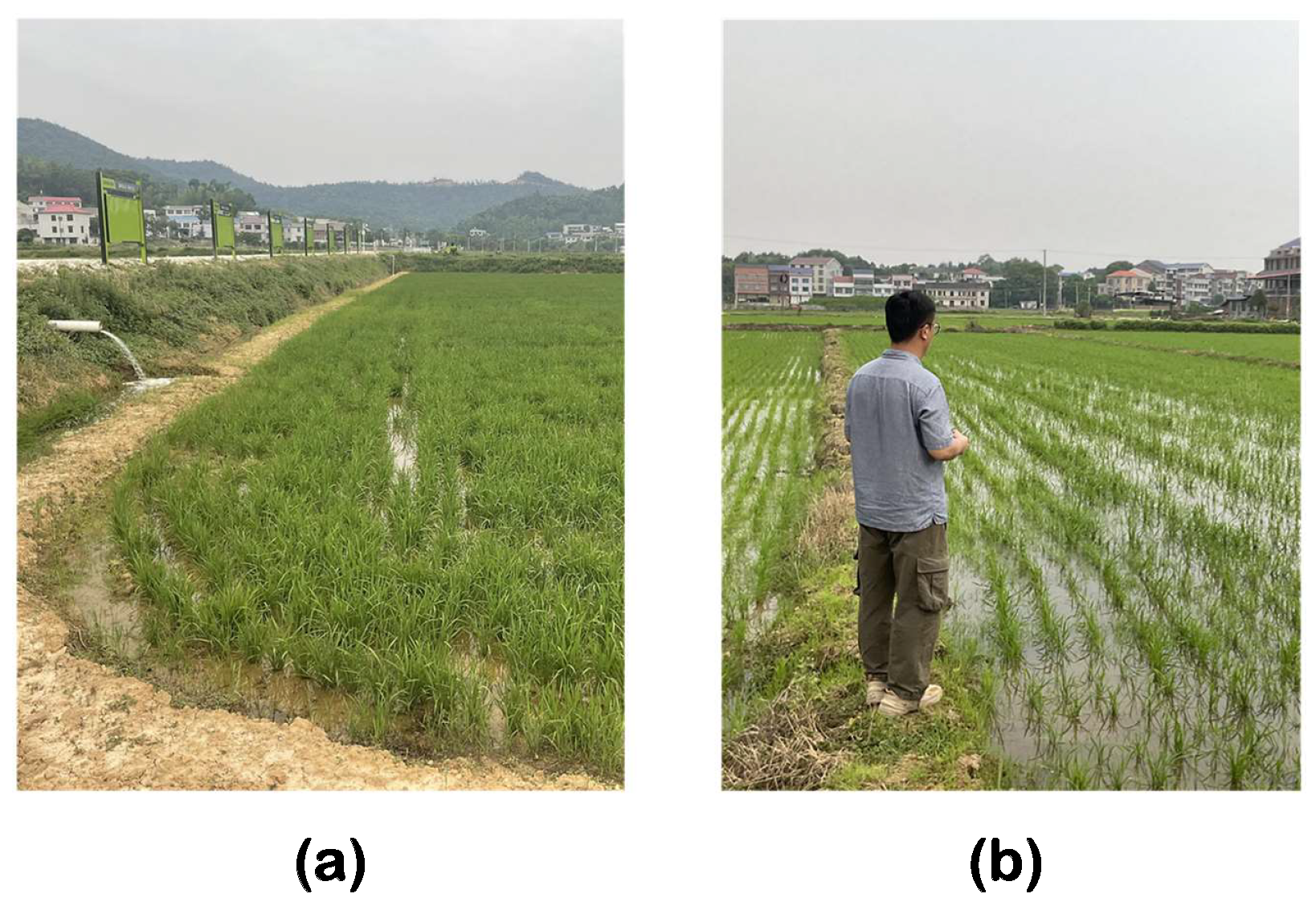
The rice field weed data were captured between April and May 2024 in two different rice fields (Zoomlion Smart Agriculture Base in Yuelu, Changsha and Yingchang Agriculture Base in Liuyang, Changsha, as shown in Figure 1).

We conducted a total of three data collection sessions. The first session took place at Zoomlion Smart Agriculture Base in Yuelu on 22 April 2024, under cloudy weather conditions, with the rice plants in the seedling stage. The second session was carried out at Yingchang Agriculture Base in Liuyang on 27 April 2024, under overcast conditions that later turned to light rain, with the rice plants in the tillering stage. The third session was conducted again at Zoomlion Smart Agriculture Base in Yuelu on 17 May 2024, under clear skies with intense sunlight, with the rice plants in the jointing stage. The images captured during these three sessions across the two locations encompass different growth stages of rice, as well as various species and distributions of weeds, along with diverse lighting conditions under different weather scenarios. Furthermore, the randomness of data distribution, varying degrees of occlusion, weed density, and different scales of photography were also considered. These measures could enhance the representativeness and generalizability of the dataset.

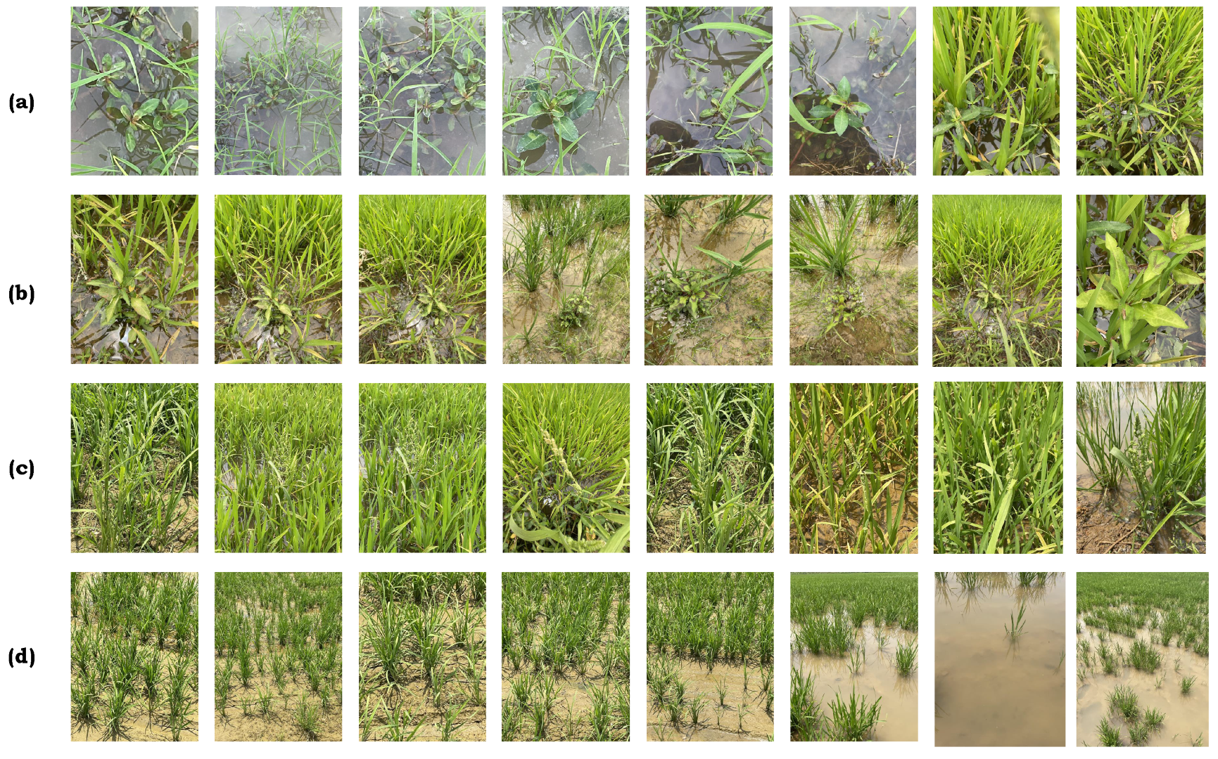
The original images had a resolution of 3024 × 4032 pixels. A total of 995 images were captured: 126 from Yingchang Agriculture Base in Liuyang and 869 from Zoomlion Smart Agriculture Base in Yuelu. These images include three common types of weeds found in the Hunan region: Beckmannia syzigachne, Alternanthera sessilis, and Polygonum lapathifolium. Some sample images from the dataset are shown in Figure 2. The data were further screened, classified, and annotated with the guidance of agricultural experts.

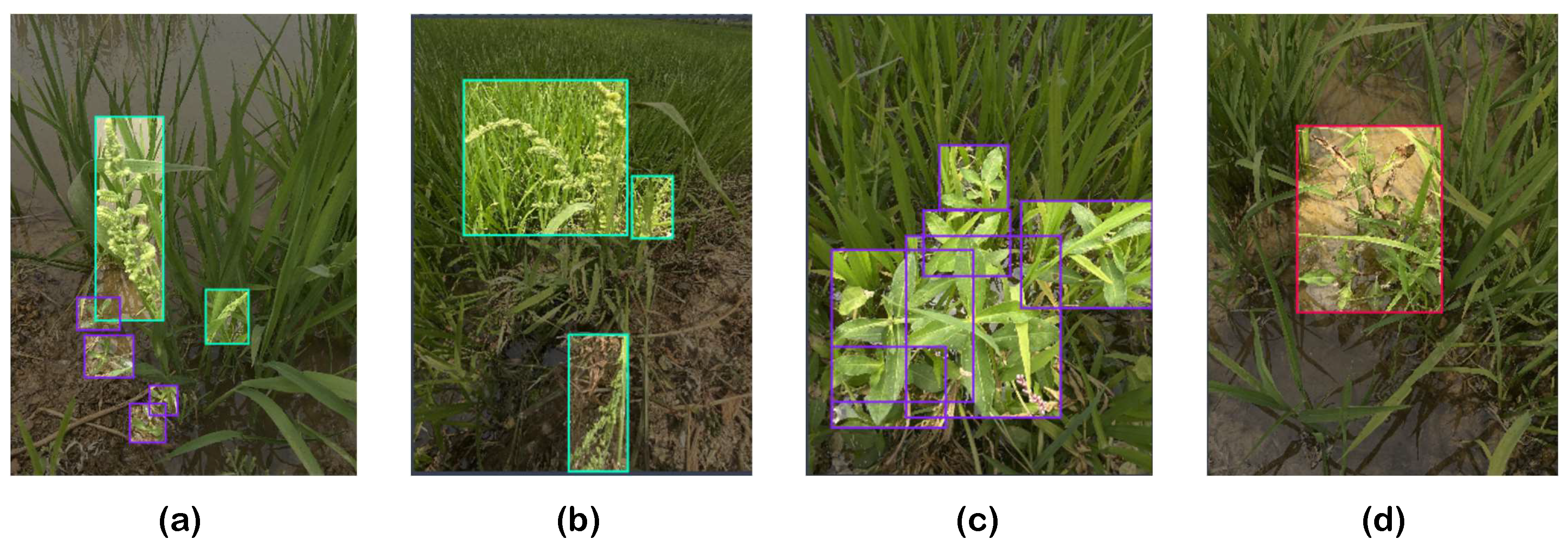
The data annotation process was conducted using the online annotation platform Roboflow. During the annotation process, the fundamental principle was to ensure that the bounding boxes precisely and completely enclosed the characteristic parts of the target weeds (such as leaves, spikes, etc.). In cases where multiple weeds were present in an image (as shown in Figure 3a), each weed was annotated separately. For scenarios with densely distributed weeds (as shown in Figure 3b,c), each individual weed was distinguished and annotated separately. In cases where weeds were partially occluded (as shown in Figure 3d), the annotation was based on the visible parts of the weeds.

To build a robust neural network, a large amount of training data are required to improve the network’s detection performance and generalization ability. Additionally, insufficient training data can make it difficult for the network to converge during training, leading to poor results. Therefore, we employed five data augmentation techniques based on the original images: flip (horizontal, vertical), rotation (between −11° and +11°), brightness (between −20% and +20%), blur (up to 0.7 px), and noise. By combining these augmentation techniques, we expanded the dataset to a total of 3297 images.

Table 1. Distribution of Weed Dataset.

Weed Species	Training Set	Validation Set	Test Set
AS	3441	672	639
PL	888	282	315
BS	2016	555	609

shows the distribution of the three types of rice field weeds and the dataset partitioning.

In the actual training process, we use AS, PL, and BS, to refer to Alternanthera sessilis, Polygonum lapathifolium, and Beckmannia syzigachne, respectively.

2.2. Network Structure of GE-YOLO

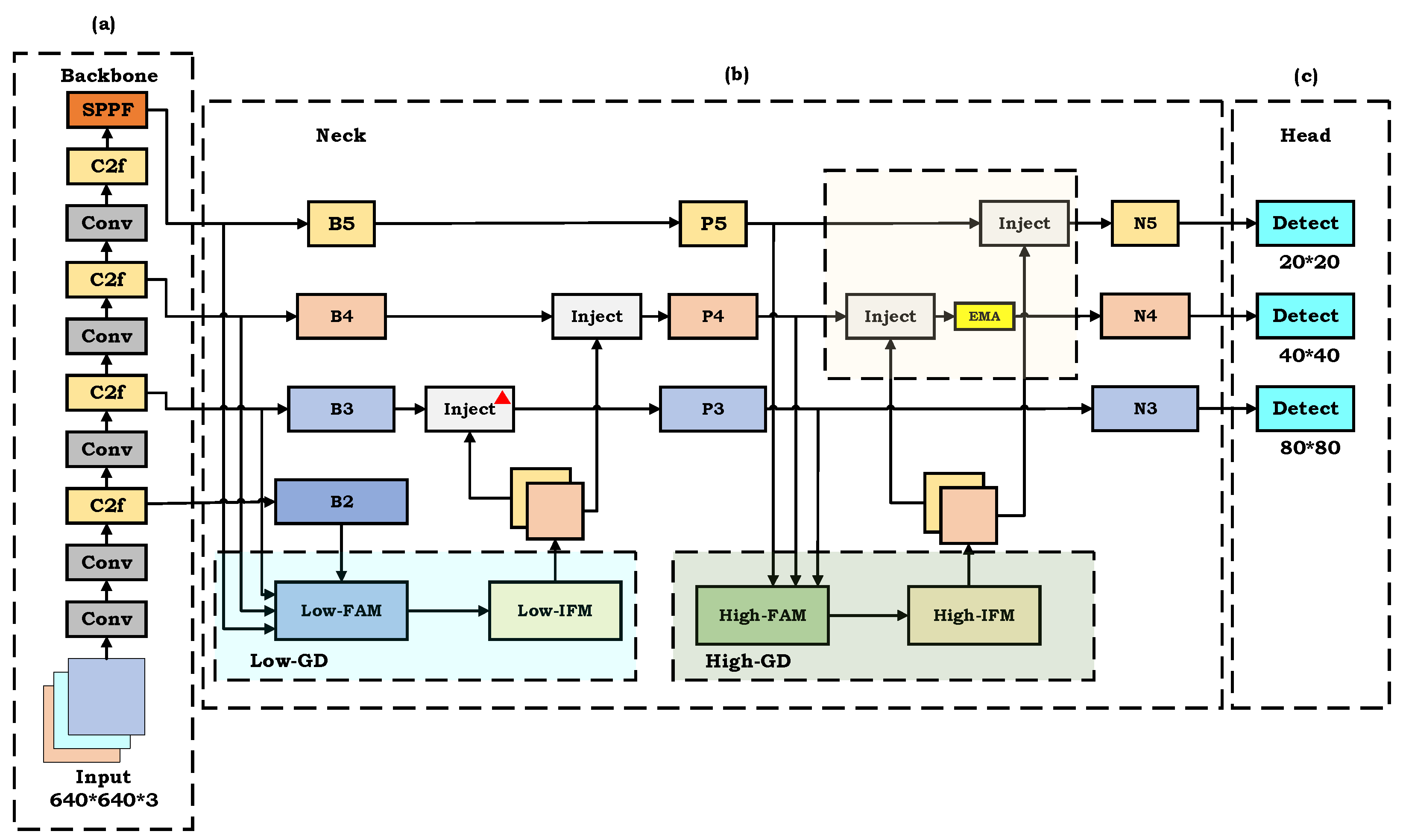
YOLOv8, known for its exceptional performance in object detection, represents a significant advancement over YOLOv5. However, when applied to the complex environment of paddy fields and the detection of multiple weed species such as AS, PL, and BS, the relatively simple structure of YOLOv8 exhibits limitations in feature extraction, distribution, and fusion. To address these shortcomings, we propose GE-YOLO, an enhanced YOLOv8 architecture, designed to improve the model’s ability to extract weed features, enhance detection accuracy, and improve generalization. GE-YOLO primarily consists of three components: Backbone, Neck, and Head. The network architecture is illustrated in Figure 4.

The Backbone is responsible for extracting deep features from the image and establishing an image feature pyramid. In the Backbone structure, we adopt the C2f structure from YOLOv8 as the core. Compared to the C3 structure, C2f is more effective in extracting weed features while reducing the number of parameters. Additionally, at the end of the Backbone, the spatial pyramid pooling fast (SPPF) structure is employed to pool weed feature maps at different scales, further enhancing the network’s ability to extract multi-scale features of weeds.

The Neck is responsible for fusing features at different scales. The Neck network of the YOLO series mostly adopts the traditional FPN structure, which merges features at different scales through multiple connecting branches. However, this structure only allows the fusion of adjacent feature layers. For non-adjacent feature layers, it can only achieve indirect fusion through recursion. This indirect method can result in slower speeds and information loss, particularly for weeds of varying scales and irregular shapes. Therefore, we adopt a new feature aggregation and distribution mechanism, Gold-YOLO [25]. This approach discards the traditional FPN structure in the Neck network and employs a gather-and-distribute mechanism. This mechanism collects and merges information from each layer and then distributes it to different network layers via the Inject module, effectively avoiding information loss and inefficiencies. Additionally, the EMA attention mechanism is integrated into the high-level aggregation and distribution branch, enabling the network to effectively perceive global and local features while maintaining computational efficiency.

The Head is responsible for generating the final detection results. The Head part retains the original design of YOLOv8, which achieves object detection through bounding box prediction, object classification, and confidence prediction.

Apart from the above measures, we also use offline data augmentation and online Mosaic data augmentation during the pre-training process to enrich sample diversity, prevent overfitting, and improve the model’s generalization ability.

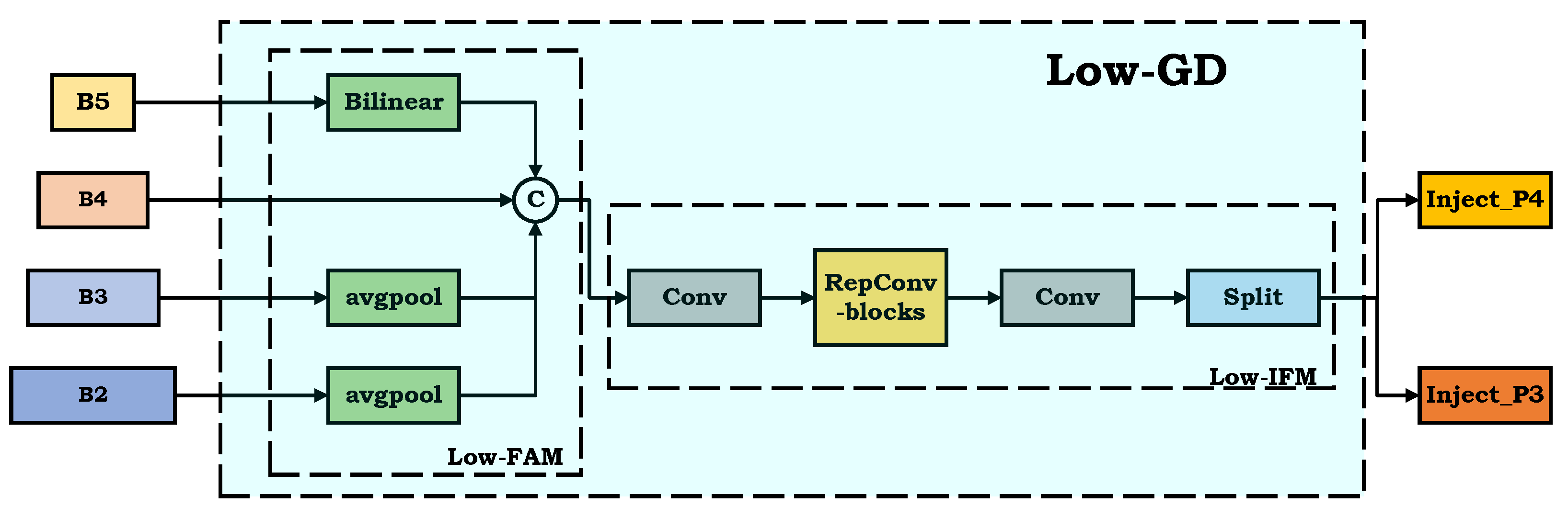
2.2.1. Low-GD

Specifically, Gold-YOLO comprises three main components: Low-GD, High-GD, and Inject. Low-GD is illustrated in Figure 5.

Low-GD’s primary function is to efficiently aggregate and fuse low-level feature maps of varying sizes. It mainly consists of two parts: Low-FAM (feature alignment module) and Low-IFM(information fusion module). The Low-FAM module scales the feature maps to a uniform size and performs channel concatenation. This approach ensures efficient information aggregation while minimizing the computational complexity during subsequent processing by the transformer module. When choosing the alignment size, two opposing factors need to be considered: (1) Maximizing the retention of low-level features, as they contain more detailed information; (2) increasing feature map size inevitably raises computational complexity. To balance accuracy and detection efficiency, $B4$ is chosen as the unified alignment size. Feature maps larger than $B4$ are downsampled to $B4$ size using global average pooling, while feature maps smaller than $B4$, like $B5$, are upsampled to $B4$ size using bilinear interpolation. Finally, these feature maps are concatenated along the channel dimension to obtain the output feature $F_{align}$. The formula is described as follows:

$$F_{align\_Channel}=\sum (C_{B2},C_{B3},C_{B4},C_{B5})$$

(1)

Subsequently, $F_{align}$ is processed through the Low-IFM module, where it is fused using the reparameterized convolution block (RepBlock) to generate the fused feature $F_{fuse}$. This fused feature is then split along the channel dimension to produce two features, $F_{inject\_P3}$ and $F_{inject\_P4}$, which are utilized for fusion at different levels. The formulas are described as follows:

$$\begin{array}{c}\hfill F_{fuse}=RepBlock\left(F_{align}\right)\end{array}$$

(2)

$$\begin{array}{c}\hfill F_{inject\_P3},F_{inject\_P4}=Split\left(F_{fuse}\right)\end{array}$$

(3)

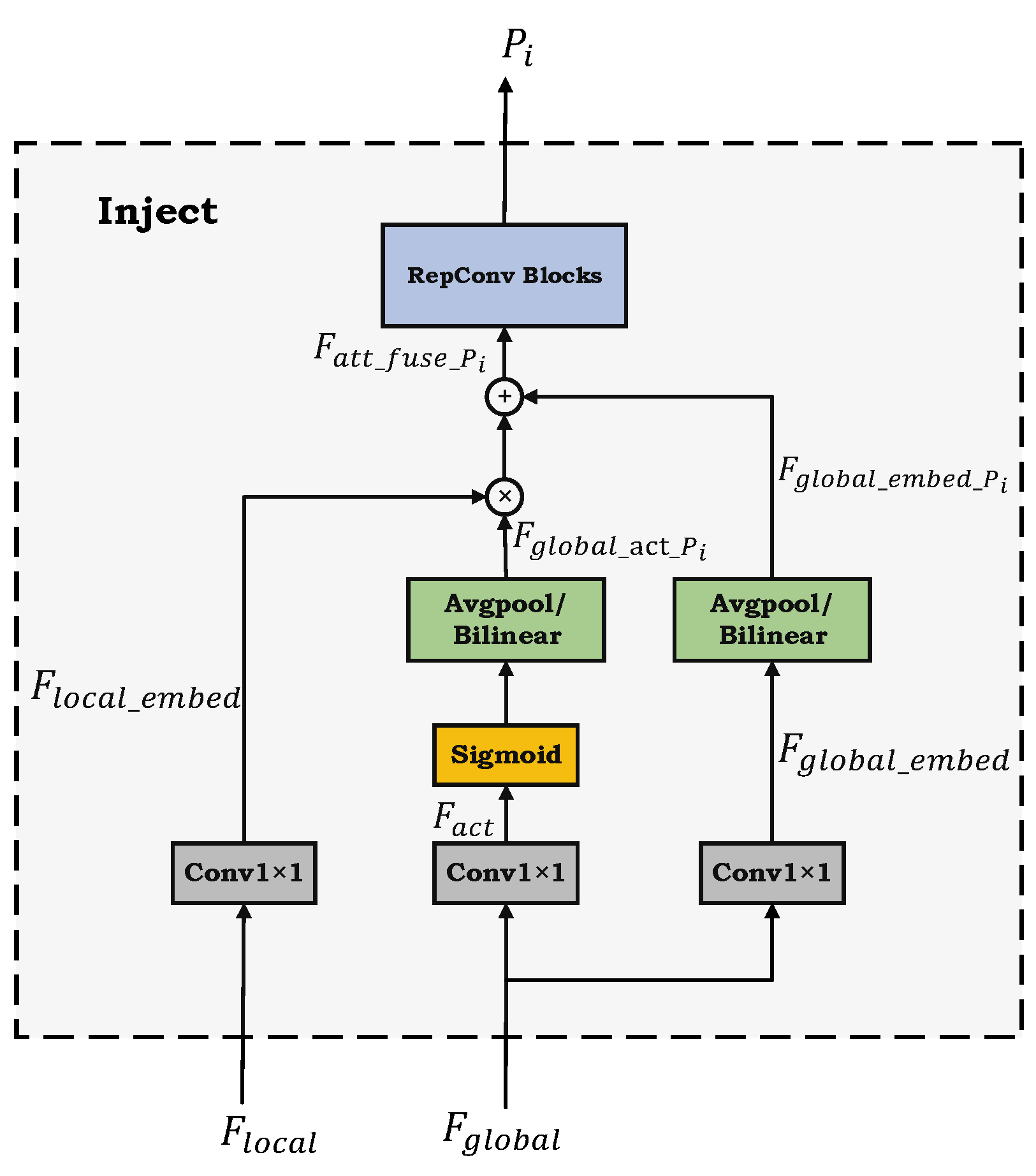
2.2.2. Inject

To facilitate the distribution of aggregated features generated by Low-GD, the Information Injection module (Inject module) is introduced to integrate global and local features. To clearly illustrate the working principle of the Inject module, please refer to Figure 6, which presents the structural diagram of the Inject module. Our explanation will focus on the Inject module marked with a red triangle (🔺) in Figure 4, which depicts the architecture of GE-YOLO.

First, the Inject module takes the local feature $F_{local}$ (denoted here as $B3$) and the global feature $F_{global}$ (denoted here as $F_{inject\_P3}$) as inputs. Second, $F_{local}$ undergoes a 1 × 1 convolution operation to generate $F_{local\_embed}$, while $F_{global}$ is processed through a branching structure, passing through two separate 1 × 1 convolution operations to generate $F_{global\_embed}$ and $F_{act}$. Third, due to the difference in spatial dimensions between the global and local features, average pooling or bilinear interpolation is applied to $F_{global\_embed}$ and $F_{act}$ to generate $F_{global\_embed\_P_i}$ and $F_{global\_act\_P_i}$, ensuring smooth integration with $F_{local\_embed}$ in the subsequent fusion process. Then, the rescaled $F_{global\_embed\_P_i}$ and $F_{global\_act\_P_i}$ are then fused with $F_{local\_embed}$. Last, the fused feature $F_{act\_fuse\_P_i}$ is further processed through the RepBlock to extract and integrate information, ultimately generating the fused feature $P_i$ (denoted here as $P3$).

The mathematical formulation corresponding to the above steps is provided as follows:

$$\begin{array}{c}{F}_{global\_act\_Pi}=resize\left(Sigmoid\left(Con{v}_{act}\left(F_{global}\right)\right)\right)\end{array}$$

(4)

$$\begin{array}{c}{F}_{global\_embed\_Pi}=resize\left(Con{v}_{global\_embed}\left(F_{global}\right)\right)\end{array}$$

(5)

$$\begin{array}{c}\begin{array}{cc}\hfill F_{att\_fuse\_Pi}& =Con{v}_{local\_embed\_Pi}\left(F_{local}\right)\hfill \\ & *F_{global\_act\_Pi}+F_{global\_embed\_Pi}\hfill \end{array}\end{array}$$

(6)

$$\begin{array}{c}{P}_i=RepBlock\left(F_{att\_fuse\_Pi}\right)\end{array}$$

(7)

By leveraging the Inject module for the distribution of aggregated features, an efficient fusion of local and global features is achieved. This enhances the network’s multi-scale feature representation capability for weed detection, enabling the model to effectively capture fine details in weed images and improve detection performance, particularly for small weed targets.

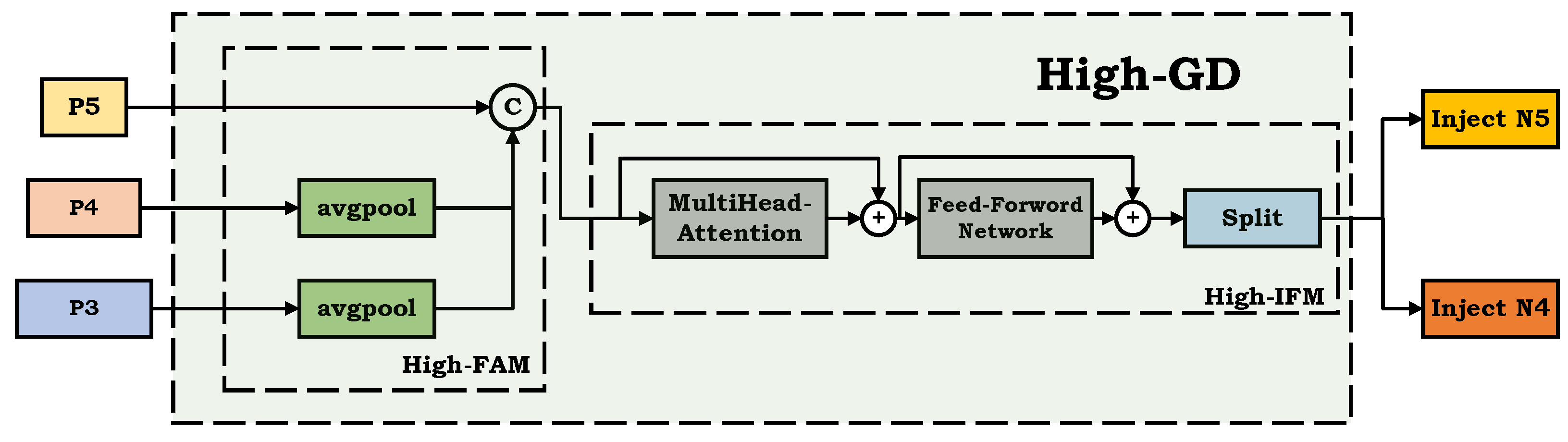
2.2.3. High-GD

High-GD is designed to further aggregate and distribute the features after the Low-GD module has fused local and global features, enriching the feature information contained in the feature maps to facilitate multi-scale weed detection in rice fields. Specifically, after completing the low-level feature aggregation and distribution process using Low-GD and the Inject module, the newly generated features $Pi$ (where $i=3,4,5$) need to undergo further high-level aggregation and distribution. This process involves the High-GD and Inject modules. The schematic diagram of the High-GD module is shown in Figure 7. Similarly, High-GD first uses High-FAM to scale the $P3$, $P4$, $P5$ features to align them. Specifically, when the sizes of the input features are $R_{P3},R_{P4},R_{P5}$, avgpool reduces the feature size to the smallest size in the feature group, $R_{P5}$. Then, the High-IFM module is used to fuse and split the aligned and concatenated features. The difference here is that the IFM module uses a Transformer module to fuse the features and generate the fused feature $F_{fuse}$. Finally, the Split operation divides $F_{fuse}$ into $F_{inject\_N4}$ and $F_{inject\_N5}$. Overall, the handling of features by High-GD can be described by the following formulas:

$$\begin{array}{c}{F}_{align}=High-FAM(P3,P4,P5)\end{array}$$

(8)

$$\begin{array}{c}{F}_{fuse}=Transformer\left(F_{align}\right)\end{array}$$

(9)

$$\begin{array}{c}{F}_{inject\_N4},F_{inject\_N5}=Split\left(Con{v}_{1x1}\left(F_{fuse}\right)\right)\end{array}$$

(10)

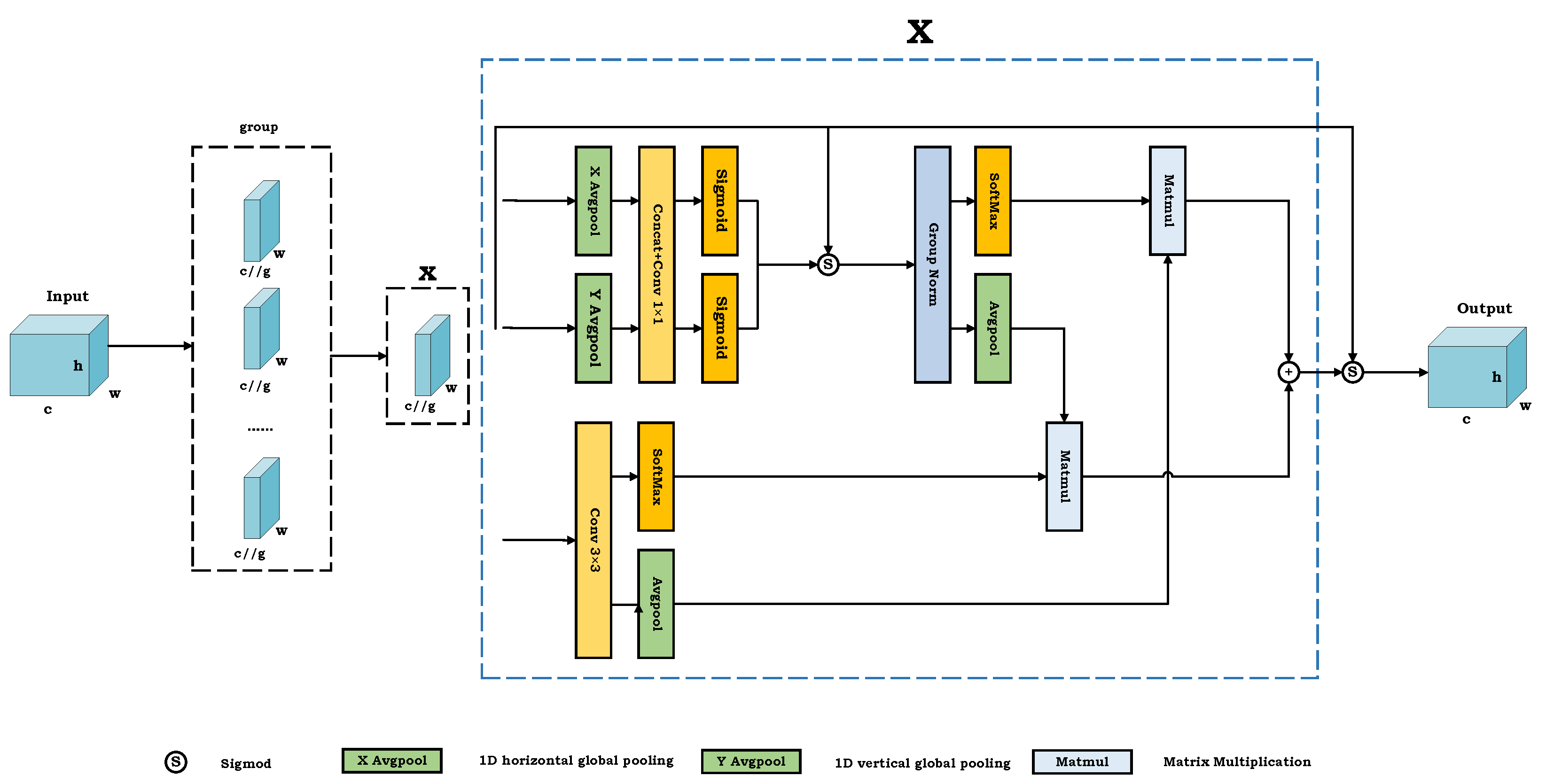
2.2.4. Efficient Multi-Scale Attention Module

In the actual weed images, the vegetative environment is often quite complex, with factors such as rice occlusion and the similarity in color between weeds and crops affecting detection performance. The addition of an attention mechanism can enhance the network’s focus on important features in the image, eliminating interference from irrelevant background elements and thereby improving detection performance.

Traditional conventional channel and spatial attention mechanisms have demonstrated significant efficacy in enhancing the discriminative power of feature representations. However, they often bring side effects in extracting deep visual representations due to channel dimensionality reduction when modeling cross-channel relationships. To address this issue, Daliang Ouyang, Su He, Jian Zhan, and others proposed the EMA attention mechanism [26]. This attention mechanism rearranges some channels into multiple batches and groups the channel dimensions into multiple sub-features, ensuring that spatial semantic features are well distributed within each feature group while reducing computation overhead. The architecture of the EMA attention mechanism is depicted in Figure 8, where h denotes the image height, w indicates the image width, c represents the number of channels, and g signifies the channel grouping.

Specifically, the EMA attention mechanism utilizes a parallel substructure that aids in minimizing sequential processing and reducing the network’s depth. This module is capable of performing convolutional operations without diminishing the channel dimensionality, allowing it to effectively learn channel representations and generate improved pixel-level attention for high-level feature maps.

The EMA module is intended to effectively model both short-term and long-term dependencies, thereby improving performance in computer vision tasks. It comprises three parallel branches, with two residing in the $1\times 1$ branch and one in the $3\times 3$ branch. The $1\times 1$ branch applies two separate 1D global average pooling operations to encode channel information along two spatial axes, while the $3\times 3$ branch employs a single $3\times 3$ kernel to extract multi-scale features. To retain channel-specific information and minimize computational load, the EMA module reorganizes certain channels into batch dimensions and divides the channel dimensions into multiple sub-groups, ensuring an even distribution of spatial semantics across each feature group. Additionally, cross-dimensional interactions are utilized to aggregate the outputs of the two parallel branches, enabling the capture of pairwise pixel relationships at the pixel level. As shown in Figure 4, To enhance the network’s attention to weed features and mitigate the impact of irrelevant backgrounds on weed detection, we introduced the EMA attention mechanism after the Inject module in the Neck network.

2.3. GIOU

In the YOLOv8 network, the default bounding box regression loss is complete intersection over union(CIOU). CIOU, building upon IOU, takes into account the distance between bounding box centers and aspect ratios, offering a more comprehensive measure for bounding box regression loss. However, CIOU introduces additional computational overhead due to the inclusion of center point distance and aspect ratio calculations. On the other hand, generalized intersection over union(GIOU) [27] has a relatively lower computational complexity and provides smoother gradient information beneficial for optimization. Therefore, we attempted to use GIOU due to its lower computational complexity and achieved better testing results compared to CIOU on the dataset. The formula for the GIOU loss function is described as follows:

$$\begin{array}{cc}\hfill GIoU& =IoU-{\displaystyle \frac{|C\setminus (A\cup B\left)\right|}{\left|C\right|}}\hfill \end{array}$$

(11)

$$\begin{array}{cc}\hfill GIoULoss& =1-GIoU\hfill \end{array}$$

(12)

Here, IoU refers to intersection over union. A represents the predicted bounding box, B denotes the ground truth bounding box, and C is the smallest enclosing rectangle that covers both bounding boxes A and B, $|A\cup B|$ denotes the area of the union of bounding boxes A and B, $\left|C\right|$ represents the area of the smallest enclosing rectangle C, $|C\setminus (A\cup B\left)\right|$ indicates the area within C that does not belong to $A\cup B$.

2.4. Experimental Environment and Model Evaluation

The hardware used for training the model includes an Intel(R) Xeon(R) Platinum 8336C CPU @ 2.30GHz and an NVIDIA GeForce RTX 4090 GPU. The programming environment used is Ubuntu 22.04.4 LTS, Python 3.9, and CUDA 11.8. During training, the model uses the Stochastic Gradient Descent (SGD) optimizer with a learning rate of 0.01 and a momentum of 0.937. The model is trained for a total of 100 epochs. Additionally, the batch size is set to 8, the number of workers is set to 8, and the weight decay is fixed at 0.0005. The performance metrics used for evaluating the model are as follows:

$$\begin{array}{cc}\hfill P& ={\displaystyle \frac{TP}{TP+FP}}\times 100\%\hfill \end{array}$$

(13)

$$\begin{array}{cc}\hfill R& ={\displaystyle \frac{TP}{TP+FN}}\times 100\%\hfill \end{array}$$

(14)

$$\begin{array}{cc}\hfill AP& ={\int }_0^{1}P\left(R\right)dR\times 100\%\hfill \end{array}$$

(15)

$$\begin{array}{cc}\hfill mAP& ={\displaystyle \frac{{\sum }_{n=1}^{3}A{P}_n}{3}}\times 100\%\hfill \end{array}$$

(16)

$$\begin{array}{cc}\hfill F1Score& ={\displaystyle \frac{2\times R\times P}{R+P}}\hfill \end{array}$$

(17)

In this context, true positive ($TP$) refers to the number of correctly identified positive samples, false positive ($FP$) refers to the number of negative samples incorrectly identified as positive, and false negative ($FN$) refers to the number of positive samples incorrectly identified as negative. Average precision ($AP$) is the area under the precision–recall curve, where n denotes the number of weed categories. mean average precision (mAP) is the average of $AP$ values across multiple categories. The F1 score is the harmonic mean of precision and recall. Additionally, we also consider the number of model parameters (Params), giga floating-point operations per second (GFLOPs), and detection frame rate (FPS).

3. Results and Discussions

3.1. Comparative Analysis of the Improvement Strategies

We propose a rice field weed detection network, GE-YOLO, which introduces the Gold-YOLO feature aggregation and distribution network, EMA attention mechanism, and GIoU loss function based on the YOLOv8 network structure. To rigorously evaluate the effectiveness of these improvements, we conducted a series of comparative experiments, testing different attention mechanisms, loss functions, and feature fusion strategies.

Specifically, we compared five different attention mechanisms: EMA, AcMix [28], CBAM [29], ECA [30], and GAM [31]. These attention mechanisms were incorporated into the GE-YOLO network at the same position as the EMA attention mechanism, serving as replacements for the EMA attention mechanism. The performance metrics obtained were then compared, and the experimental results are presented in

Table 2. Comparison of Different Attention Mechanisms.

Strategy	Precision/%	Recall/%	mAP/%	F1Score/%	GFLOPs	Params/M	Speed/FPS
AcMix	92.1	87.9	92.1	90.0	17.8	8.12	55.9
CBAM	93.7	86.3	92.7	89.8	17.7	8.08	85.8
ECA	92.7	87.1	92.8	89.8	17.6	8.06	86.4
GAM	90.9	86.9	92.4	88.9	19.0	8.47	84.3
EMA	92.1	88.6	93.1	90.3	17.6	8.06	85.9

.

From the experimental results, it can be observed that, for both mAP and F1 score metrics, the EMA attention mechanism achieved the best performance among all the attention mechanisms. In terms of the number of parameters and computational complexity, the network with the EMA attention mechanism also had the lowest values. Regarding inference speed, the network with the EMA attention mechanism achieved 85.9 FPS, only slightly lower than the network with the ECA attention mechanism. After considering the trade-off between efficiency and accuracy, we conclude that the EMA attention mechanism is the optimal choice.

We also tested five different loss functions (EIoU [32], SIoU [33], WIoU [34], and CIoU, GIoU) on the GE-YOLO network to compare the performance metrics. The experimental results are presented in

Table 3. Comparison of Different Loss Functions.

Loss function	Precision/%	Recall/%	mAP/%	F1Score/%	GFLOPs	Params/M	Speed/FPS
EIoU	92.2	84.3	90.8	88.1	17.7	8.06	92.2
SIoU	92.0	87.2	91.8	89.5	17.7	8.06	90.6
WIoU	59.4	75.7	69.4	66.6	17.7	8.06	84.5
CIoU	90.9	87.0	91.7	88.9	17.6	8.06	87.3
GIoU	92.1	88.6	93.1	90.3	17.6	8.06	85.9

.

From the experimental results, it can be seen that the network using the GIoU loss function achieved the best performance in both mAP and F1 scores. Although the inference speed (FPS) was slightly lower than that of the EIoU and SIoU networks, the GIoU loss function led to a significant improvement in weed detection accuracy. After considering the trade-off, we conclude that it is the optimal choice.

To address the low resolution of small objects during multi-scale feature fusion, we also tested two different feature fusion strategies: the Gold-YOLO feature aggregation and distribution network and the bidirectional feature pyramid network (BiFPN) [35]. In this process, the GIoU loss function was kept constant, and the EMA attention mechanism was added at similar positions. The relevant performance metrics obtained from the comparative experiments are presented in

Table 4. Comparison of Different Feature Fusion Strategies.

Strategy	Precision/%	Recall/%	mAP/%	F1Score/%	GFLOPs	Params/M	Speed/FPS
None	93.1	84.2	91.6	88.4	8.2	3.15	192.1
BiFPN	91.2	88.4	92.2	89.8	8.1	2.57	122.7
Gold-YOLO	92.1	88.6	93.1	90.3	17.6	8.06	85.9

.

Based on the results of the comparative experiments, we found that the Gold-YOLO network leads to a significant increase in network parameters and a reduction in inference speed. However, Gold-YOLO achieves relatively high weed detection accuracy, and the FPS can still reach 85.9. After weighing the trade-offs, we chose Gold-YOLO as the improvement strategy for the original feature fusion network of YOLOv8. The use of BiFPN is also worth further investigation.

Additionally, the backbone network of YOLOv8 may generate lower-resolution feature maps when handling small objects. Therefore, we further explored the possibility of improving the backbone network. We tested five different improvement strategies to enhance the conventional convolution operations in the YOLOv8 backbone, including LDConv [36], CG Block [37], RFAConv [38], RepNCSPELAN4 [18], and ODConv [39]. The experimental results are presented in

Table 5. Comparison of Different Backbone Network Improvement Strategies.

Strategy	Precision/%	Recall/%	mAP/%	F1Score/%	GFLOPs	Params/M	Speed/FPS
LDConv	88.3	86.1	90.5	87.2	17.1	7.82	28.6
CG Block	91.3	85.6	91.4	88.4	16.5	7.64	69.6
RFAConv	94.1	85.8	92.1	89.8	16.5	8.10	71.8
RepNCSPELAN4	93.5	87.2	92.3	90.2	16.3	7.63	76.5
ODConv	88.4	85.1	91.1	86.7	16.7	9.23	72.7
None	92.1	88.6	93.1	90.3	17.6	8.06	85.9

.

From these data, it can be concluded that although these modules theoretically improve the feature extraction performance of the backbone network, the actual test metrics (such as mAP and F1 scores) do not perform as well as the original GE-YOLO. Additionally, in terms of FPS, GE-YOLO also achieved the highest value. Therefore, we decided to retain the original structure of the backbone network and continue using the native YOLOv8 backbone network.

The results of the above comparative experiments provide a comprehensive validation of the proposed improvements, demonstrating their effectiveness in enhancing the network’s robustness and accuracy, particularly in the application of rice field weed detection tasks.

3.2. Model Validation and Comparison with Other Algorithms

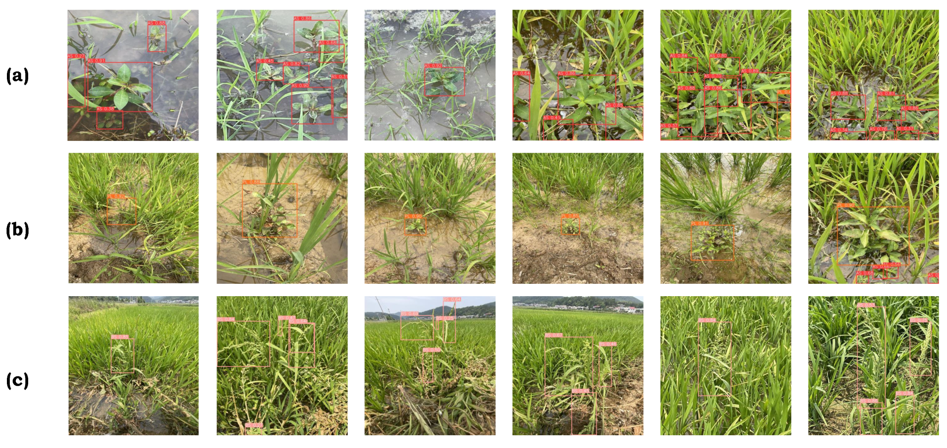
The detection results of GE-YOLO are shown in Figure 9. As illustrated, GE-YOLO effectively detects multi-scale objects, including densely packed targets. This demonstrates that our model performs well in handling different sizes of weed targets and in detecting weeds with dense distributions. To further validate the efficacy of GE-YOLO, we compared its performance with that of other mainstream object detection algorithms. The detailed experimental results are presented in

Table 6. Results of different algorithms.

Model	Precision/%	Recall/%	mAP/%	F1Score/%	GFLOPs	Params/M	Speed/FPS
RT-DETR	25.9	16.7	12.1	20.35	103.4	31.99	14.6
YOLOv3	91.8	86.5	91.4	89.13	282.8	103.667	17.2
YOLOv4	79.4	79.9	83.9	79.65	119.7	52.5	-
YOLOv5	91.1	86.7	92.2	88.85	7.1	2.5	140.3
YOLOv6	92.8	84.8	91.0	88.71	11.8	4.23	170.3
YOLOv7	86.7	87.1	89.8	86.9	105.1	37.2	-
YOLOv8	92.5	84.8	91.2	88.49	8.1	3.01	187.6
YOLOv9	96.0	85.5	91.9	90.45	102.3	25.32	30.9
YOLOv10	90.6	82.5	90.3	86.64	98.7	20.46	-
YOLOv11	94.1	85.2	91.7	89.4	6.4	2.59	-
GE-YOLO(Ours)	92.1	88.6	93.1	90.3	17.6	8.06	85.9

. From the results in Table 6, it is evident that GE-YOLO achieves a higher level of performance compared to other YOLO series algorithms in terms of both mAP and F1 Score. The mAP reaches 93.1%, which is the highest among all compared algorithms. The F1 Score is 90.3%, surpassing all other compared algorithms except YOLOv9. Although our model slightly lags behind YOLOv9 in terms of F1 Score, it offers a lower parameter count, reduced computational complexity, and higher FPS. Therefore, overall, our model demonstrates superior performance and high reliability in the task of weed detection in rice fields.

3.3. Ablation Experiments

To validate the effectiveness of GE-YOLO, we conducted ablation experiments. The results are shown in

Table 7. Results of ablation experiments.

Model	Gold-YOLO	GIoU	EMA	mAP/%	F1Score/%	GFLOPs	Params/M	Speed/FPS
YOLOv8	-	-	-	91.2	88.5	8.1	3.01	187.6
YOLOv8	✓	-	-	92.1	89.3	17.6	8.06	96.0
YOLOv8	✓	✓	-	92.2	89.4	17.6	8.06	92.5
YOLOv8	✓	✓	✓	93.1	90.3	17.6	8.06	85.9
Increase				↑1.9	↑1.8	-	-	-

.

Based on the results of the ablation experiments, it is evident that the model’s mAP and F1 Score improve significantly with the incorporation of various enhancements. Starting with the YOLOv8 baseline model, we introduced Gold-YOLO to the Neck network. This modification resulted in improvements in both mAP and F1 Score, reaching 92.1% and 89.3%, respectively, which represents an increase of 0.9% and 0.8% compared to the baseline model.

Next, using GIOU loss function further enhanced the mAP and F1 Score by 0.1% each. Finally, The addition of the EMA attention mechanism contributed an additional 0.9% improvement in both mAP and F1 Score, reaching 93.1% and 90.3%, respectively. From the results of the ablation experiments, it can be observed that the introduction of the Gold-YOLO feature fusion and distribution mechanism, as well as the EMA attention mechanism, led to a decrease in FPS. Through analysis, we believe this is likely due to the increased number of model parameters resulting from the incorporation of the feature fusion and distribution mechanism and the EMA attention mechanism. These additional parameters require computation during the inference process, thereby prolonging the inference time and causing a drop in FPS. However, by accepting this computational cost, the model’s detection metrics, such as mAP and F1 score, have been significantly improved. Moreover, GE-YOLO ultimately achieves 85.9 FPS, far exceeding the real-time requirement of 25 FPS. Therefore, GE-YOLO is capable of handling real-time detection tasks while maintaining high detection accuracy.

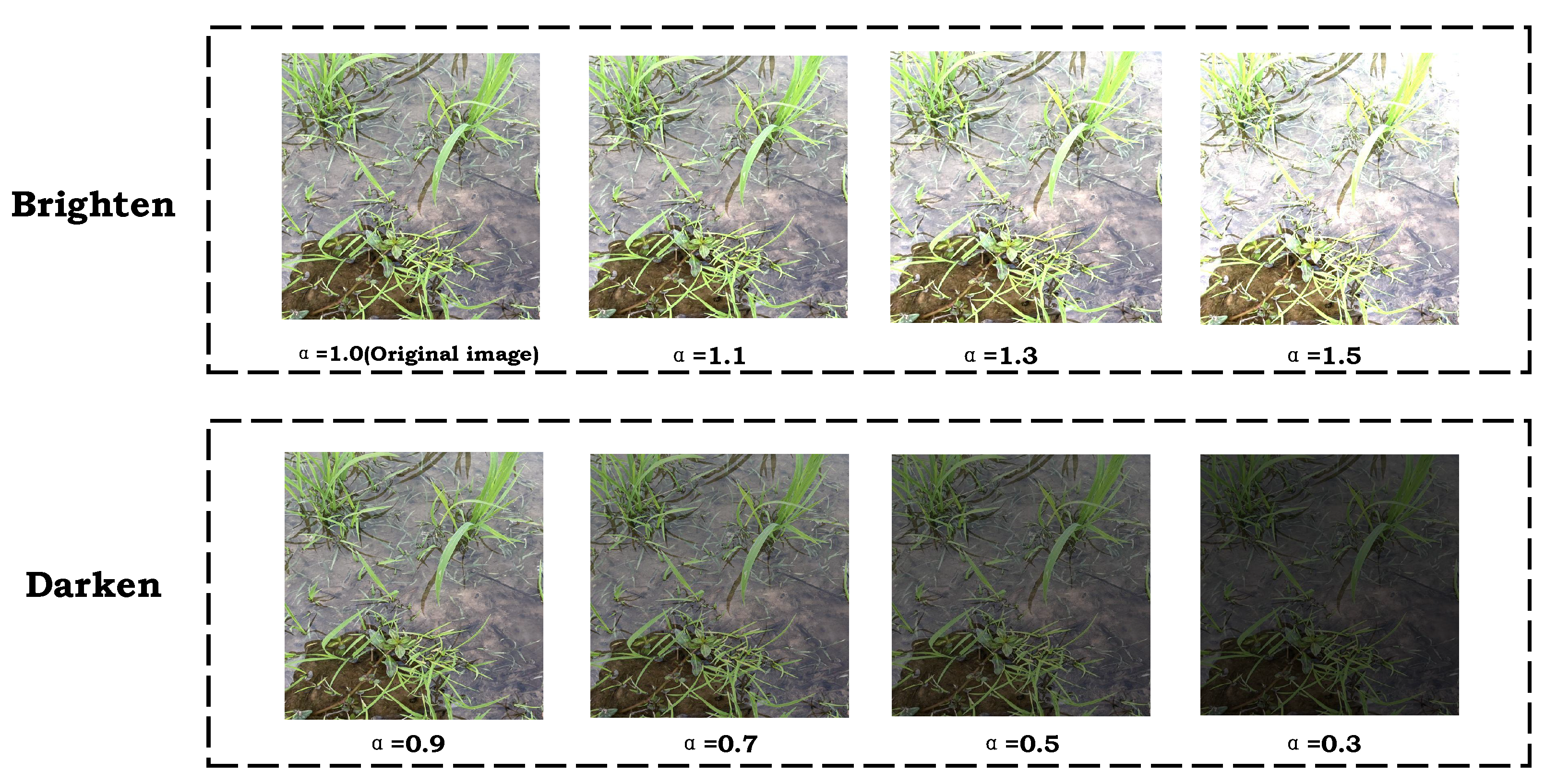
3.4. Testing Under Different Lighting Conditions

In real-world scenarios, lighting conditions can vary significantly. For instance, overcast weather or dusk can result in dim lighting, while intense sunlight can lead to overly bright conditions. To evaluate the robustness of our proposed model, we simulated different lighting scenarios by varying the illumination factor $\alpha$ and assessed our model’s performance under these conditions. The description of lighting simulation is as follows:

$$\begin{array}{c}\hfill I_{new}(x,y)=\alpha I_{raw}(x,y)\end{array}$$

(18)

Here, $I_{raw}(x,y)$ represents the pixel value of the original image at position $(x,y)$. The illumination factor $\alpha$ is used to adjust the brightness, where $\alpha >1$ indicates an increase in brightness, $0<\alpha <1$ indicates a decrease in brightness, and $\alpha =1$ means no change in brightness. $I_{new}(x,y)$ represents the pixel value of the adjusted image at position $(x,y)$. Images under different illuminations are shown as Figure 10.

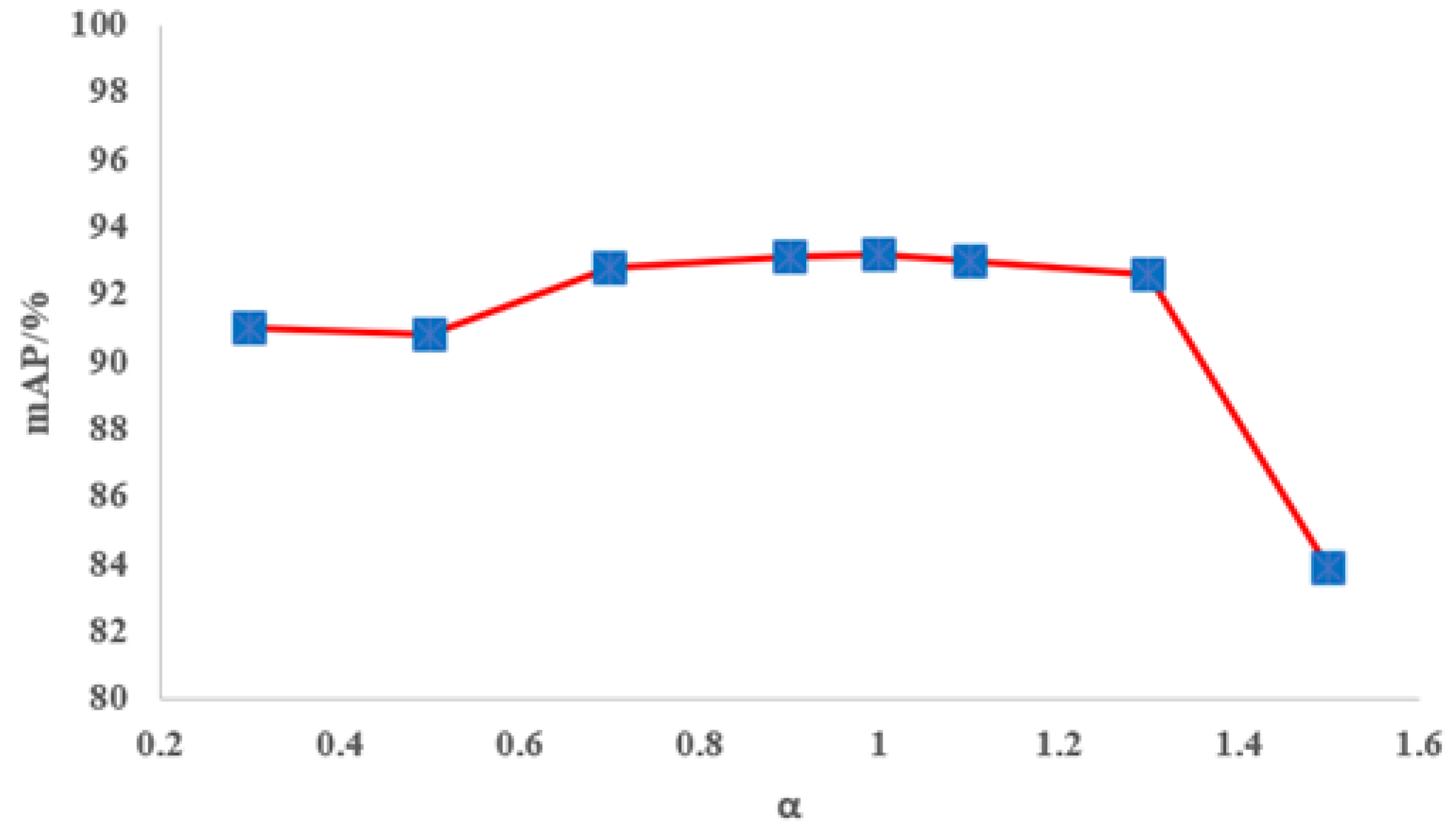
We set multiple values of $\alpha$ and obtained a series of test results as shown in Figure 11. It can be observed that our model remains stable when $\alpha$ is within the range of 0.3 to 1.1, with the mAP value consistently above 90%. Although as $\alpha$ increases further, the mAP value gradually declines, but it is still above 82%. This indicates that our model has good resistance to low light and moderate bright light conditions, demonstrating strong generalization performance.

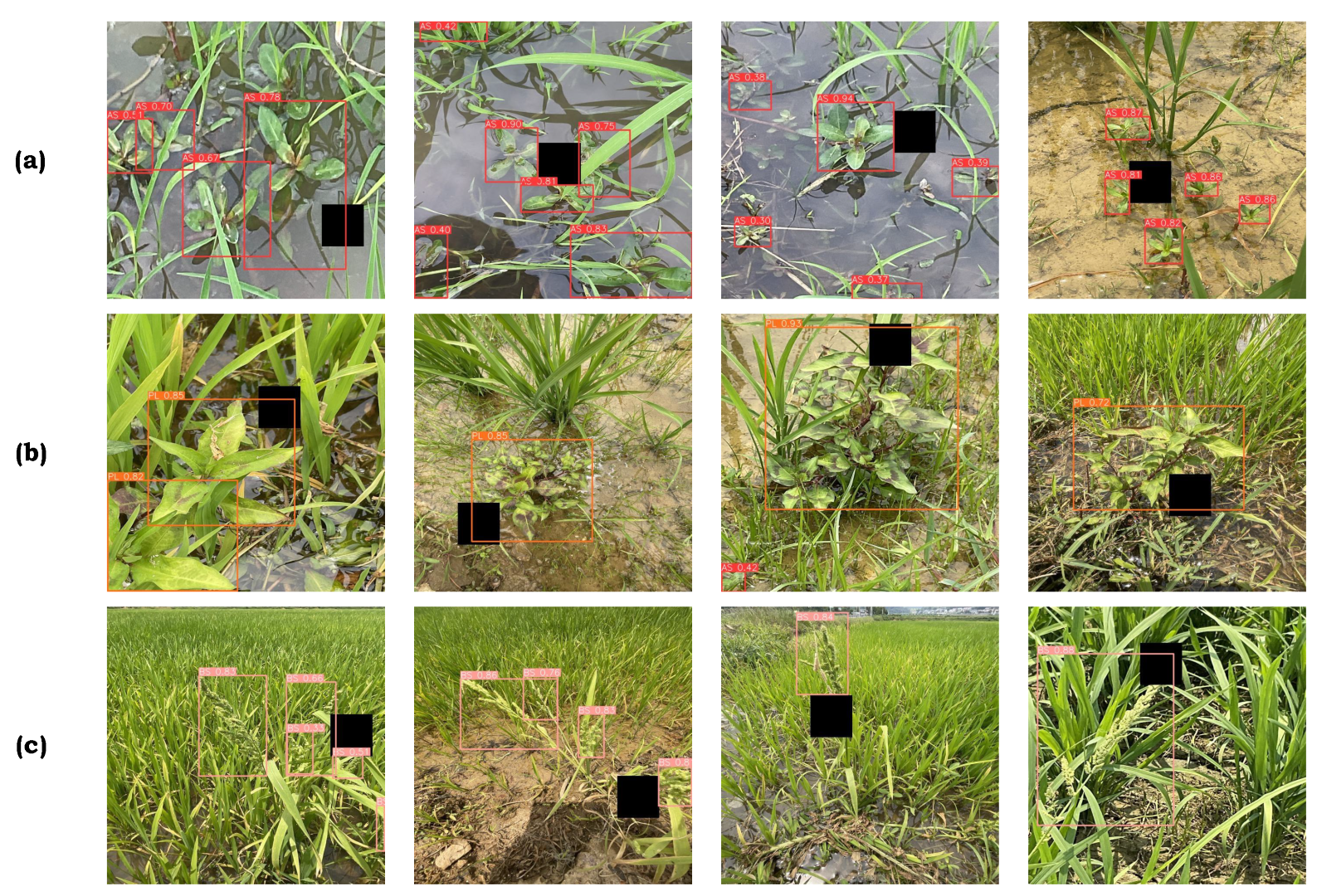
3.5. Testing in Occluded Conditions

In actual rice paddy environments, the distribution of weeds is often irregular and mixed with crops, resulting in common occurrences of occlusion between crops and weeds, as well as between different weeds. Therefore, to address this issue and evaluate the generalization performance of our model under occlusion conditions, we further processed the dataset by artificially creating occlusion regions on the original images. Occluded images and some of the resulting detection results are shown in Figure 12.

From the detection results shown in

Table 8. Weed detection results under occlusion conditions.

Weed Species	Precision/%	Recall/%	mAP/%
ALL Species	90	81.6	88.7
AS	88	72.3	82.1
PL	91.3	92.5	95.3
BS	90.7	80	88.7

and Figure 12, it is evident that GE-YOLO performs well in detecting weeds under high occlusion conditions. The average mAP for all weeds reaches 88.7%, and each weed species achieves an mAP of over 80%. This demonstrates that the proposed model has strong performance in handling weed detection tasks with occlusion.

3.6. Discussion

To date, while research on weed detection in rice fields has made some progress, challenges such as complex vegetation environments, water surface reflections, and weeds with similar shapes and colors to crops remain unresolved. The generalization and robustness of existing algorithms need further enhancement. In response, we have proposed GE-YOLO, a network specifically designed for detecting weeds in rice paddies, capable of handling various weed targets under different sizes, lighting conditions, and occlusions.

Our network incorporates several innovative mechanisms to enhance robustness and generalization: (a) GE-YOLO introduces a feature fusion distribution network that directly performs multi-scale feature fusion, effectively enhancing the network’s ability to represent and detect weed targets of different scales in complex environments. This enables the network to maintain high precision and consistency in detection performance across various scales, types of weeds, and shooting angles. (b) GE-YOLO incorporates an EMA mechanism that strengthens the network’s focus on target regions within the feature maps. This allows the network to accurately identify weed regions even in complex environments where weeds and rice exhibit similar colors and significant overlap. (c) GE-YOLO adopts the GIoU loss function, which provides smoother gradient information and lower computational complexity. This optimization directs the network’s performance toward effectively identifying weeds in paddy fields under complex conditions, making it better suited for the task of weed detection in rice fields.

Moreover, through our field efforts, we have constructed a high-quality dataset of rice paddy weeds that encompasses diverse growing environments, various growth stages of rice, different lighting conditions under varying weather, as well as varying weed densities and distributions. Our network effectively learns the features of the three common weed species in Hunan rice fields: Alternanthera sessilis, Polygonum lapathifolium, and Beckmannia syzigachne, which are visually similar to rice crops. The experimental results also validate that our model exhibits excellent robustness and generalization capabilities.

However, there are some limitations to our research. Due to practical constraints, we have only collected data for three common weed species. In reality, there are additional weed species in rice fields that vary by regional environment. The common weed species need detection in rice fields also include Echinochloa crus-galli, Monochoria vaginalis, Cyperus rotundus, Cyperus serotinus, Commelina communis, Potamogeton distinctus, and Lemna minor. Therefore, we plan to expand our dataset in future research. Additionally, there is still room for improvement in our model, and we will continue to explore ways to enhance it to better suit various rice field weed detection tasks.

4. Conclusions

Our research aims to propose a high-precision and robust rice field weed detection network. To this end, we collected weed data from rice fields under varying conditions, covering three weed species: Beckmannia syzigachne, Alternanthera sessilis, and Polygonum lapathifolium. We introduced an improved weed detection network, GE-YOLO. The experimental results demonstrate that GE-YOLO achieves a remarkable 93.1% mAP, 90.3% F1 Score, and 85.9 FPS in weed detection tasks. It effectively detects weeds of various sizes and outperforms all other mainstream detection networks. Additionally, GE-YOLO exhibits excellent generalization and high reliability under varying lighting conditions and occlusions. This suggests significant potential for GE-YOLO in agricultural production and weed management.