Investigation of the Mechanical and Magnetic Property Changes in Austenitic Stainless Steel AISI 304 After Cold Rolling Under Various Heat Treatment Conditions

Abstract

This study systematically investigates the influence of heat treatment on the mechanical and magnetic properties of AISI 304 austenitic stainless steel following cold rolling. Experimental analyses were conducted on samples annealed at 50 °C to 1200 °C in 25 °C increments. The mechanical properties were characterized through chemical and metallographic analyses, microhardness testing, hardness measurements, and tear-off force evaluations. Magnetic properties were assessed using a fluxgate sensor to analyze the intrinsic magnetic field variations. The findings reveal that the magnetic field intensity peaks at an annealing temperature of 100 °C, followed by a progressive decline up to 700 °C. A pronounced reduction in magnetic properties was observed at 500 °C, with stabilization beyond 700 °C. Notably, the increase in magnetic field intensity at 100 °C suggests a potential transformation of deformation-induced martensite back into austenite. These results provide insights into the thermal stability of cold-rolled AISI 304 stainless steel and its structural evolution, contributing to a deeper understanding of its mechanical and magnetic behavior under varying heat treatment conditions.

1. Introduction and Related Works

As the global population ages, diseases affecting the musculoskeletal, cardiovascular, and nervous systems are becoming increasingly prevalent. Lifestyle factors such as elevated stress levels, unhealthy dietary habits, and reduced physical activity further exacerbate these health concerns. Musculoskeletal disorders significantly impact a large portion of the global population, leading to 20an increasing demand for implantable medical devices designed to improve patient’s quality of life. Consequently, research in this field is crucial for advancing clinical practice and enhancing treatment options.

The incidence of musculoskeletal and cardiovascular diseases is rising both globally and in Slovakia, primarily due to increased life expectancy and various lifestyle and environmental factors. This trend underscores the urgent need for medical advancements to address the growing burden of chronic illnesses. In Slovakia, the population aged 70 and above has grown significantly, reaching 174,000 in 2016. The average life expectancy increased to 76.9 years by 2020, and the adult obesity rate reached 19% in 2019 [1,2]. Chronic conditions such as osteoporosis, osteoarthritis, and rheumatoid arthritis severely impact individuals’ quality of life. Additionally, traffic accidents pose a significant public health concern, with the World Health Organization (WHO) estimating 1.3 million fatalities and 20–50 million non-fatal injuries worldwide by 2025 [3]. Addressing these challenges is essential to improving the well-being of affected individuals.

In response to these medical needs, biomaterial research has gained considerable attention. Scientists focus on developing advanced materials with improved properties, cost-effectiveness, and enhanced biocompatibility. The integration of new biomaterials into medical practice has the potential to significantly reduce the complications associated with traditional implantable devices [4,5]. Interest lies in biomaterials with reactive and sensory capabilities, which can improve patient outcomes. Developing biocompatible biomedical materials involves interdisciplinary collaboration among material scientists, biomedical engineers, medical doctors, biotechnologists, and biologists. This multidisciplinary approach aims to enhance the feasibility of production while improving patients’ living conditions [6,7].

Due to their essential properties, austenitic stainless steels (ASSs) are among the most widely used materials for orthopedic applications. Their mechanical strength and corrosion resistance make them suitable for long-term implantation in the human body. These steels exhibit high corrosion resistance and non-magnetic characteristics, making them ideal for magnetic resonance imaging (MRI) techniques. Common biomedical grades, such as AISI 316L (American Iron and Steel Institute) and ASTM F55 (American Society for Testing and Materials), typically contain 17–20% Cr, 12–15% Ni, and 2–3% Mo. The presence of molybdenum enhances corrosion resistance, while chromium contributes to passivation. ASSs cannot be hardened through heat treatment but can be mechanically strengthened via cold deformation techniques [8,9,10]. Although they exhibit reduced resistance to stress corrosion cracking (SCC), pitting, and intergranular corrosion, they offer superior resistance to bodily fluid-induced corrosion and demonstrate excellent biocompatibility. Their strength, flexibility, and ease of shaping make them ideal for orthopedic implants such as hip, knee, and joint replacements, where durability and resistance to repetitive mechanical loads are essential.

Despite their favorable properties, austenitic steels are not without limitations. Long-term performance in physiological conditions remains a key concern, as mechanical stress and environmental exposure can affect their durability [11,12]. Prolonged use can lead to material wear, potentially releasing metal particles into the surrounding tissues, which may cause inflammation, bone loss, and implant failure. Additionally, these steels may corrode in high-chloride or acidic environments, compromising implant integrity over time. Fatigue and mechanical stress can further weaken the material, forming cracks and eventual structural failure [13,14].

The causes of endoprosthesis failure have evolved. Historical data suggest that some failure mechanisms have been mitigated through implant design and material selection improvements [15,16]. Data from the Norwegian Hip Registry indicate that aseptic loosening decreased between 1987 and 2007, attributed to the widespread use of well-documented implants. However, during the same period, infection rates and dislocation cases increased. Preventing implant failure remains a crucial priority, as inadequate material quality can lead to fatigue and cracking [17,18]. Early diagnosis is essential to avoid complete failure, and a thorough understanding of materials science and electromagnetism can aid in detecting potential damage at an early stage [19].

Ref. [20] studied the effect of crack tip constraint in terms of the thickness and initial crack size on the failure behavior of AISI 316L. Fracture tests were performed, and the crack extension for the resistance curve method due to deviating from the standard was evaluated. The failure of the samples was also assessed using the Failure Assessment Diagram (FAD). The results showed that unloading compliance underestimates the crack extension in the presence of significant plastic deformation of the samples and that the plastic collapse occurs in all samples before the crack grows in the blunting regime.

Another research group investigated the effects of tempering and cryogenic heat treatment on grain orientation and a few key mechanical parameters of austenitic stainless steel 304. The experiment outcomes demonstrated that various heat treatment techniques can be used to modify and enhance the mechanical properties of AISI 304 to suit a particular need. Their findings demonstrated that in comparison to tempered samples, which provided the best tensile strength, hardness, and minimum percentage of elongation in length value, cryogenically treated samples exhibited the lowest tensile strength, hardness, and highest percentage of elongation value [21].

In refs. [22,23], a failure investigation of a cemented femoral stem hip implant made of double-tapered stainless steel 316L was carried out. Fracture tomography, visual observations, material characterization, and morphological analysis were performed to verify fatigue as the failure mechanism. The fatigue initiation point was a surface flaw or defect that formed an indentation on the upper portion of the stem’s neck. The pattern of the beach markings, which showed the development of two separate regions, “rough” and “smooth”, which evolved more quickly and slowly, respectively, indicates that low cycle loads were most likely the cause of the failure.

The impact of deformation on the magnetic characteristics of high interstitial steel FeCr18.2Mn18.9–0.96C + N at low temperatures was examined in ref. [24]. Tensile testing started at room temperature and stopped at 10, 20, and 30% deformations. Vibrating Sample Magnetometry (VSM) was used to quantify magnetic fields. Microstructural, morphological, and crystalline structural investigations revealed that the material was homogeneous and stably austenitic in structure, lacking α- or ε-martensite. Below Neel temperature, the material displays a paramagnetic/antiferromagnetic transition. It was measured that the distorted material’s magnetization and magnetic susceptibility had decreased. The magnetic contribution was determined to impact the SFE of about 5 mJ/m².

Ref. [25] examined the impact of austenite stability on the microstructure and mechanical characteristics of three types of austenitic stainless steel during cold rolling. Samples with varying grain sizes characterized the microstructures during deformation. The strain hardening behavior of the three stainless steel sheets used in this study shows that martensite and grain size strengthening contributed to the case of the two 304 stainless steel sheets. In contrast, in the case of the 316 stainless steel sheets, only grain size contribution was found.

Ref. [26] evaluated the effect of plastic deformation on austenitic steel using electromagnetic nondestructive evaluation (eNDE) techniques. The goal was to differentiate various levels of plastic deformation in conductive biomaterials. Two instruments were used: the GF708 magnetic field sensor (Sensitec GmbH, Mainz, Germany) and the Magnet Physik device (Dr. Steingroever GmbH, Magnet-Physik, Cologne, Germany), which measures remanence and coercivity up to 200 °C. A light microscope aided in deformation analysis. The results showed that plastic deformation below 5% was undetectable. Three-dimensional scanning provided new insights into the magnetic behavior of specimens. The study confirmed that mechanical and electromagnetic properties co-vary, and detecting plastic deformation in AISI 304 depends on the appropriate sensing method.

This article explores changes in the mechanical and magnetic properties of biocompatible steel AISI 304 that have been mechanically processed and subjected to various thermal treatments. It presents measurements evaluating the selected mechanical parameters and intrinsic magnetic fields for electrically conductive material. The results are compared and critically evaluated, and new insight is gained in the quantitative nondestructive evaluation of the investigated structure. The novelty of this article can be considered the systematic investigation of the influence of heat treatment on the mechanical and magnetic properties of AISI 304. There is a focus on a comprehensive analysis of the relationship between heat treatment and material properties after strain hardening, which is not usually covered in detail. Several analytical procedures are used in the solution: the research includes mechanical (microhardness, strength, tensile strength) and magnetic (internal magnetic field) measurements, thus providing a more comprehensive view of the behavior of the steel at different temperatures. At the same time, a detailed analysis of the influence of temperature on magnetic properties is presented. In contrast to conventional studies, which often use wider temperature ranges, in this study, the samples were analyzed with acceptable resolution (25 °C steps from 50 °C to 1200 °C), which allows for a more detailed identification of changes in structure and properties. The results can be used to optimize the heat treatment of austenitic steels in technical and biomedical applications, where monitoring their mechanical and magnetic properties is essential.

2. Experimental Setup, Methods, and Procedures

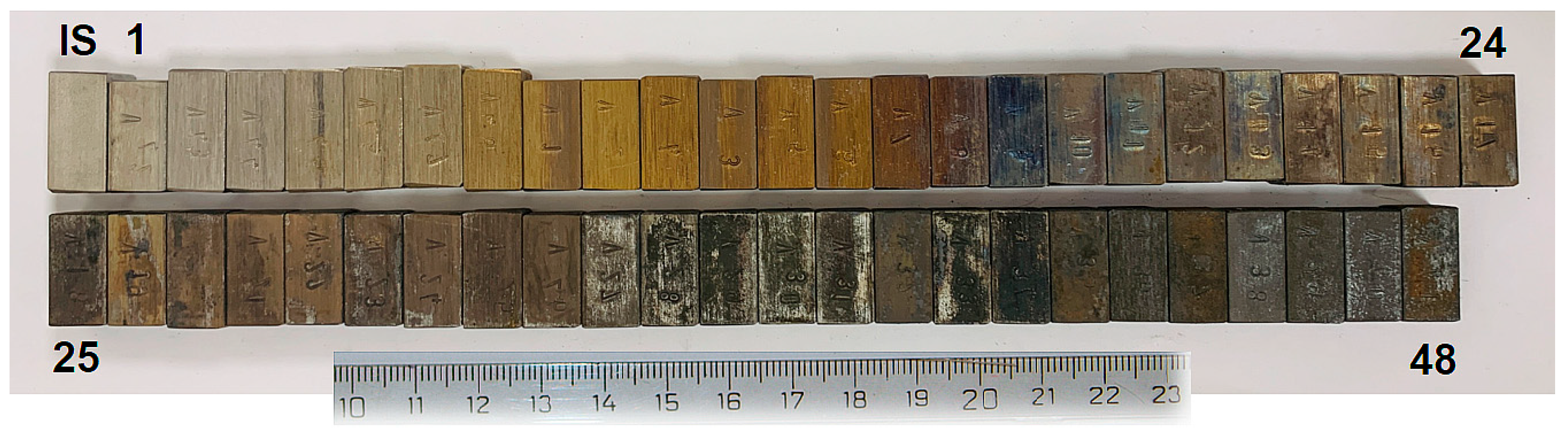
We utilized various investigative methods and procedures based on different physical principles to analyze and investigate changes in the mechanical and magnetic properties of ASSs. This knowledge base will be valuable for improving the production processes of implantable biocompatible substitutes and ensuring their functionality and quality. Our experiments included measurements of mechanical parameters (microhardness, hardness, and tear-off force) and measurements of the intrinsic magnetic field of the samples using a suitable sensor for measuring weak magnetic fields. The investigation focused on analyzing material samples made of austenitic stainless steel, specifically grade AISI 304. The samples were originally part of a square bar measuring 10 mm $\times$ 10 mm $\times$ 3000 mm, which was subsequently cut into smaller pieces approximately 20 mm in size. Before the cutting process, the bar underwent plastic deformation from longitudinal cold rolling in one direction. The analysis was performed on samples that were annealed at various temperatures ranging from 50 to 1200 °C in increments of 25 °C for 30 min each. Each cut sample underwent different heat treatments using the annealing process. In total, 49 samples were prepared (one sample in the initial state and forty-eight samples after heat treatment). Each sample was labeled with a numerical code stamped directly on the sample wall for clear identification at high processing temperatures, as seen in Figure 1. Controlled heating, temperature resistance, and rapid water cooling were used to achieve material structure homogenization and eliminate any influences previously caused by the manufacturing process. During cold rolling, the steel undergoes plastic deformation. Annealing reduces the areas affected by plastic deformation and leads to a more uniform structure by dissolving carbides, oxides, sulfides, and intrusions in the steel. Rapid cooling in water prevents the further exclusion of these substances. Annealing at specific temperatures and holding times brings the steel to a more favorable thermodynamic state, and recrystallization helps reduce intrinsic stresses and eliminate deformation strengthening. Prolonged annealing leads to significant changes in the material’s properties due to the growth and coarsening of austenitic grains.

Kalling’s No. 2 Reagent (ES Laboratory LLC, Glendora, CA, USA) was used for sample preparation, which includes 2 g of CuCl₂, 40 mL of HCl (CuCl₂: copper chloride; HCl: hydrochloric acid), and 50 to 80 mL of ethanol in the stainless steel etchant.

2.1. Chemical and Metallographic Analysis

The samples were analyzed for chemical composition using a spark emission spectrometer SPECTROMAXx (SPECTRO Analytical Instruments GmbH, Kleve, Germany). The measured values, shown in

Table 1. Chemical composition of the experimental material AISI 304 compared with the standard (wt %).

	C	Mn	Cr	Si	Ni	Mo	S	P	Fe
AISI 304	0.0308	1.44	18.87	0.315	7.8	0.24	0.0493	0.0236	rest of
STN 17 240	≤0.07	≤2	17.0 ÷ 20.0	≤1	9.0 ÷ 11.5	N/A	0.03	0.045	rest of

, are compared with the material standard STN 17 240 in the Slovak Republic to ensure adherence to the required standards for maintaining material properties such as hardness and corrosion resistance.

Metallographic analysis requires properly prepared samples to observe the microstructure of materials. Initially, a long rod of the material was cut into smaller samples, rinsed with water and alcohol, and dried with warm air. Dentacryl (methyl methacrylate casting compound) and bakelite (phenol-formaldehyde polycondensate) were used to press the samples in a Struers CitoPress-1 (Struers S.A.S., Champigny-sur-Marne, France) machine for proper attachment. The next step involved grinding and polishing the samples with a Struers TegraPol-15 automatic polisher. After grinding, the samples were washed and dried, and then an etchant solution (G + HF + HNO₃; G: glycerine; HF: hydrofluoric acid; HNO₃: nitric acid) was applied to reveal the material’s structure. The microstructure of the etched stainless steel samples was examined using a NEOPHOT 32 (Zeiss AG, Oberkochen, Germany) light microscope and documented using the NIS Elements 4 (Nikon Corporation, Minato, Tokyo, Japan) program at varying magnifications. The article discusses the investigation of selected mechanical and magnetic properties.

2.2. Assembly for Measuring Microhardness and Hardness

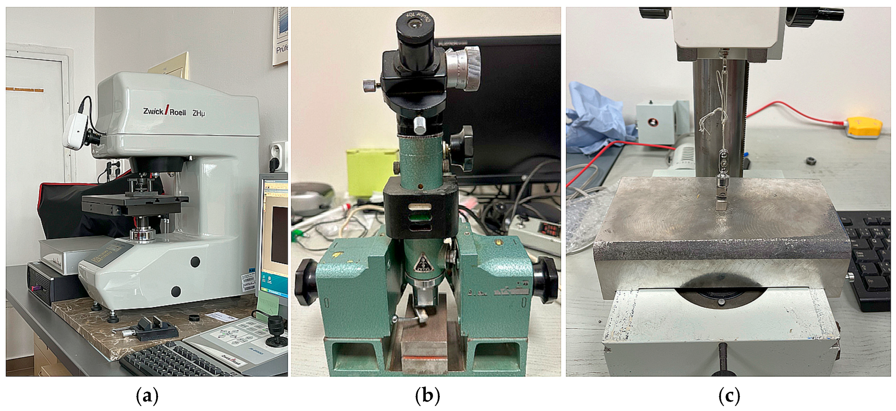
Microhardness and hardness measurements were carried out using the Vickers method. A diamond quadrilateral pyramid with an apex angle of 136° was pressed into metallographically prepared samples in their initial state, perpendicular to the rolling direction. The Zwick/Roell ZHµ microhardness tester (ZwickRoell Ltd., Ulm, Germany, Figure 2a) was used for the microhardness measurements, with a load of 0.5 kp (HV 0.5) and a 10 s load time at a room temperature of 20 °C. The measurements were taken at the center of the sample due to the expected symmetry of microhardness results from the beginning to the end of the sample. The investigation of changes in sample hardness based on annealing temperature was conducted using a hand-held Vickers hardness tester with a 10 kp load (HV 10) at a consistent load time and temperature for all measurements, as seen in Figure 2b.

2.3. Measurement of Tear-Off Force

Tear force measurement is used to test the magnetic properties of substances. It uses calibrated instruments to determine the force needed to detach a sample from a permanent magnet. This helps determine the material’s macroscopic magnetic characteristics. The force magnitude was measured using a BT 42i force sensor (CMA, Amsterdam, The Netherlands). Data from the sensor were transferred to a computer and analyzed using the Coach 6.7 program (CMA).

2.4. Measurement of the Intrinsic Magnetic Field

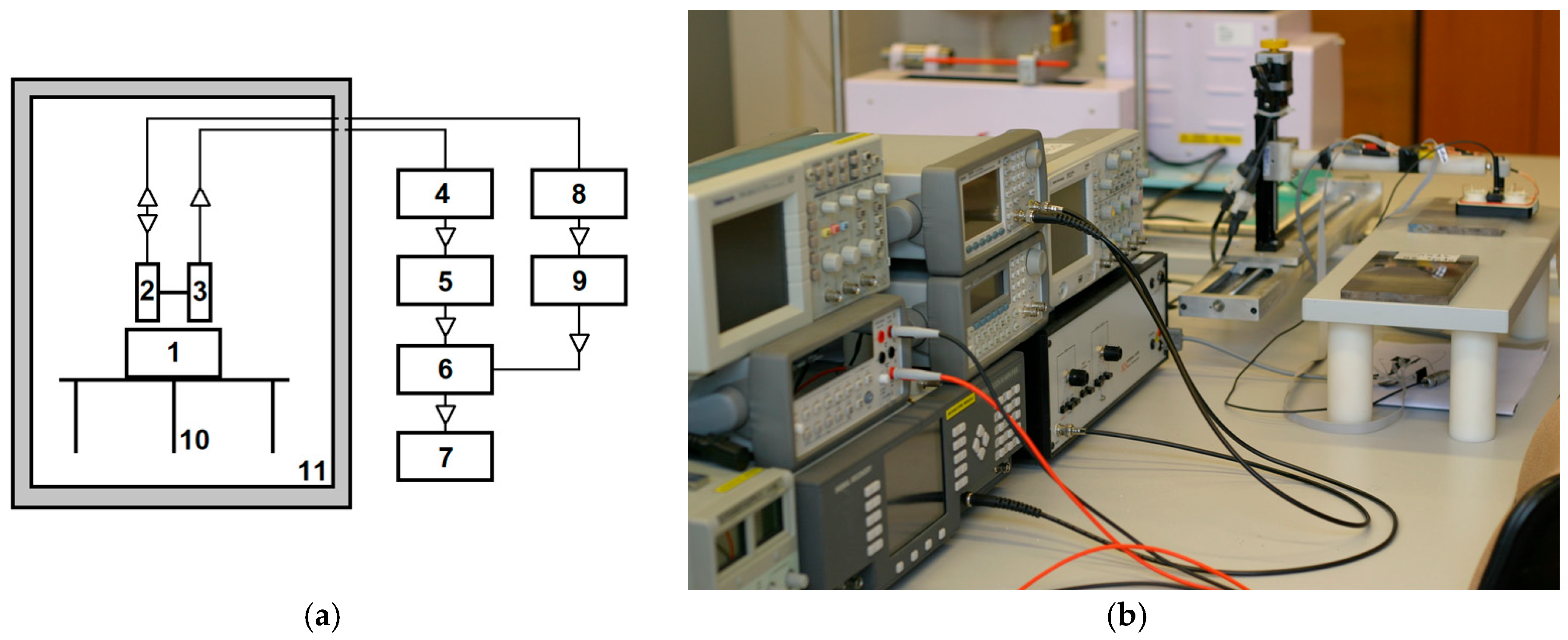
The setup for investigating the relatively weak magnetic fields of the prepared samples consists of a defined measuring apparatus, shown in Figure 3.

The samples were measured in a chamber designed to shield electromagnetic interference using a single-axis fluxgate sensor to detect weak magnetic fields. The sensor can detect magnetic field values in the 0 to 3.4 kHz frequency range and convert them into a DC electric voltage signal, as seen in Figure 4. Its response is linear within the measuring range, and it can distinguish the orientation of the magnetic field. When measuring the intrinsic magnetic field of the samples, a fluxgate sensor positioned on a printed circuit board alongside other electronic circuits sensed the DC component within the specified frequency range. It was powered by a constant 5 V DC voltage source, drawing approximately 25 mA of current during the measurement process.

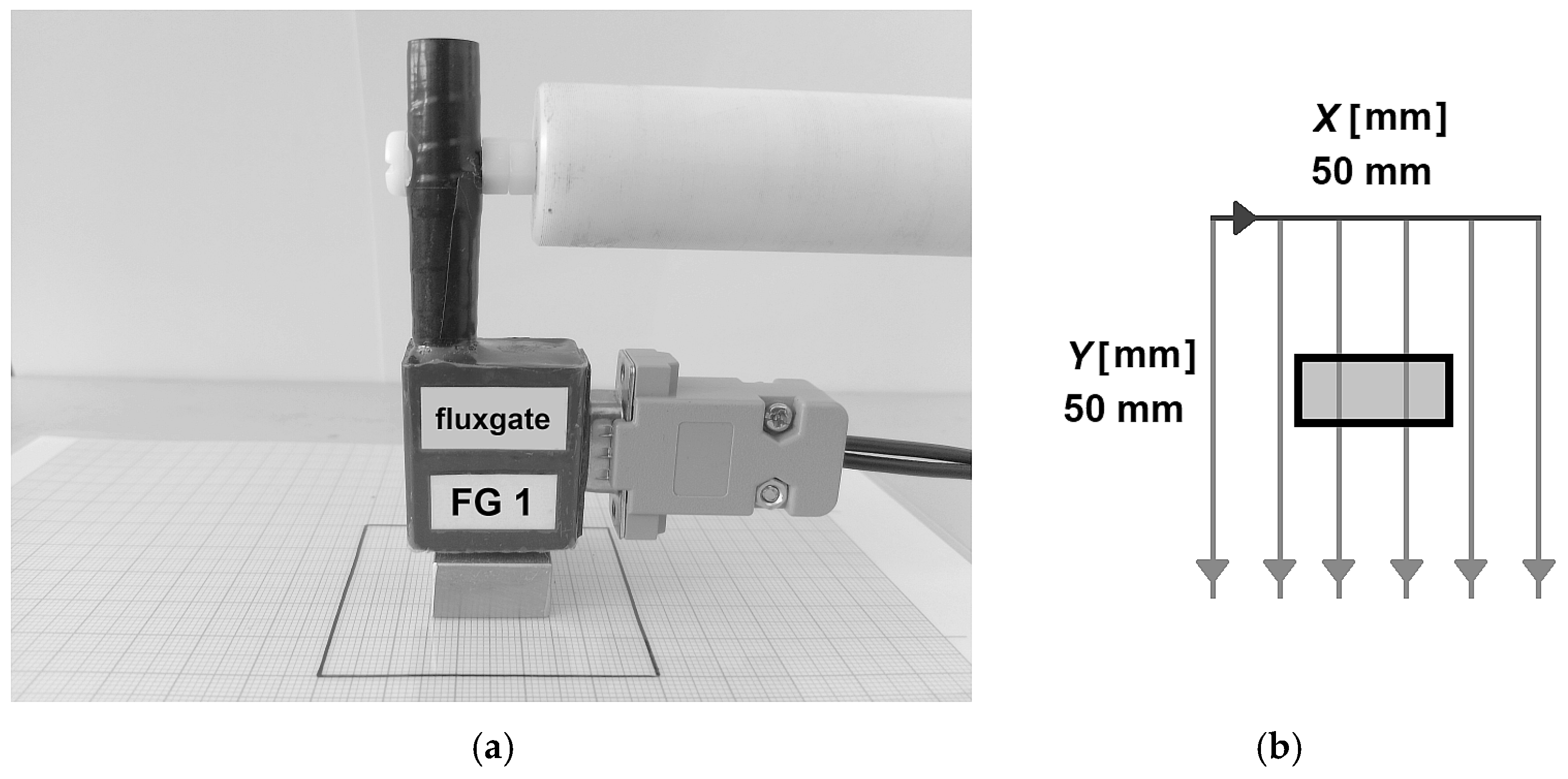
The lock-in amplifier Signal Recovery DSP 7280 (Ametek, Inc., Berwyn, PA, USA) was a selective voltmeter to filter out valuable signals. The filtered signal from the fluxgate sensor was then transmitted to the analog input of the acquisition card and processed using LabVIEW 2014 virtual instrumentation software (National Instruments, Austin, TX, USA). A program block was created in the virtual instrumentation environment to manipulate the signals, store data, and execute other necessary actions. This interface also produced control commands for a three-axis linear manipulator to which the fluxgate sensor was connected. The measurement was conducted in an EM-shielded space using a linear three-axis manipulator (Velmex Inc., New York, NY, USA) to which the sensor was attached, as seen in Figure 5a. The manipulator arm utilizes stepper motors and a threaded rod, providing a resolution of 1.2 µm on each axis, enabling precise positioning. This setup allows for the construction of a spatial map of the magnetic field near the samples under investigation. The scanning procedure in the region of interest (ROI) involved positioning the sample in the center of a 50 mm $\times$ 50 mm area, as depicted in Figure 5b.

The samples’ magnetic field was scanned using a technique called comb scanning. Data from the sensor were recorded as they moved in the y-axis direction, with 1000 readings taken for each scan line. The spacing between individual scanning lines was fixed at Δx = 0.5 mm. This means that 100 scan lines were recorded for each scan setup of one sample area, representing one complete scan cycle. After each cycle, the sensor was returned to the initial (reference) position, and the measured data were saved in a *.CSV format file. All examined samples were subjected to a non-contact evaluation, focusing on the repeatability of each measurement. Each sample was measured from both of its identical sides (faces), which were labeled L (left side) and R (right side). The experimental measurement conditions from both opposite surfaces were essentially the same. The fluxgate sensor was consistently positioned above the sample at a fixed distance from the surface; h = 1.4 mm. The valuable data were collected using a PXI 6255 digital acquisition card (DAQ) (National Instruments, Austin, TX, USA), with a sampling frequency of fs = 10 kHz.

3. Experimental Results and Analysis

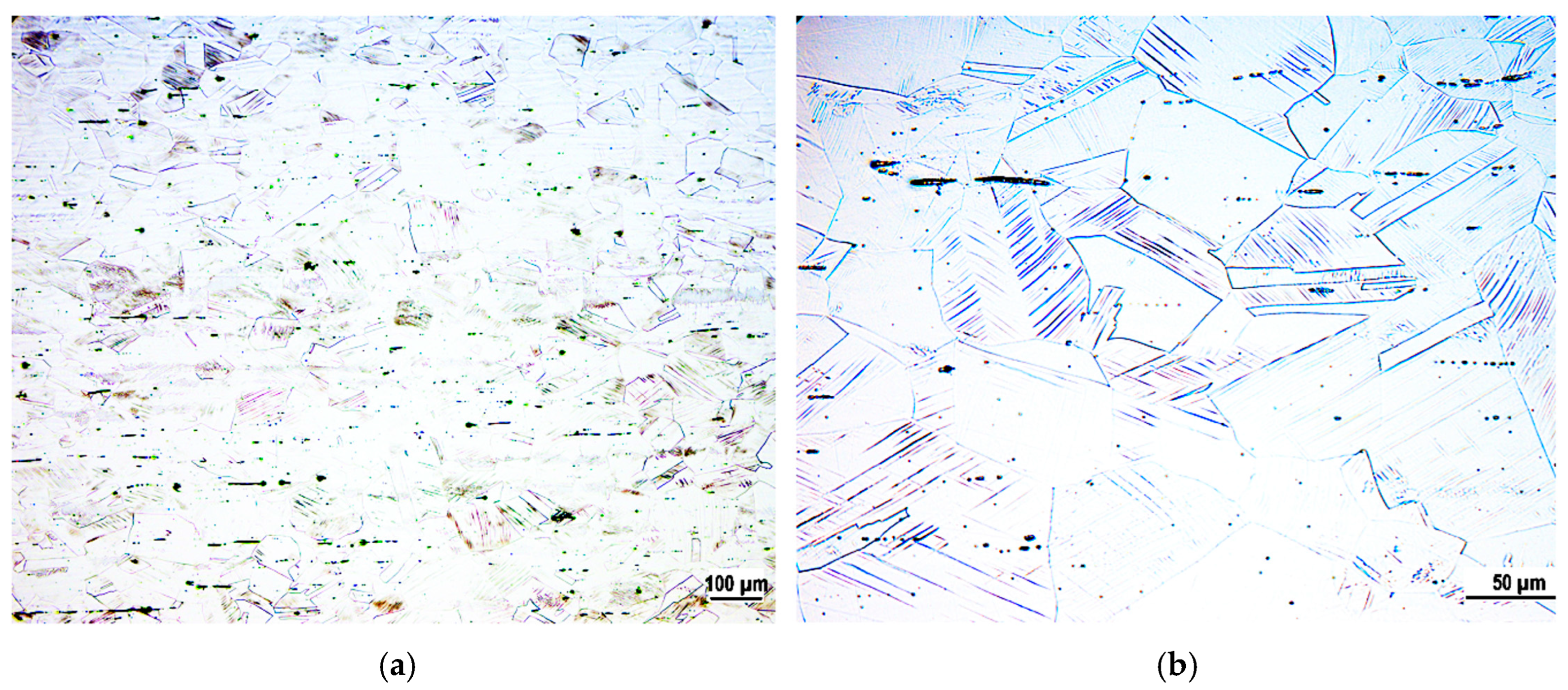
This section summarizes the measurement results and compares them with the available theoretical knowledge. We used a light microscope to analyze the microstructure of the initial state samples of AISI 304. The material structure consists of polyhedral austenite grains of various sizes, as shown in Figure 6.

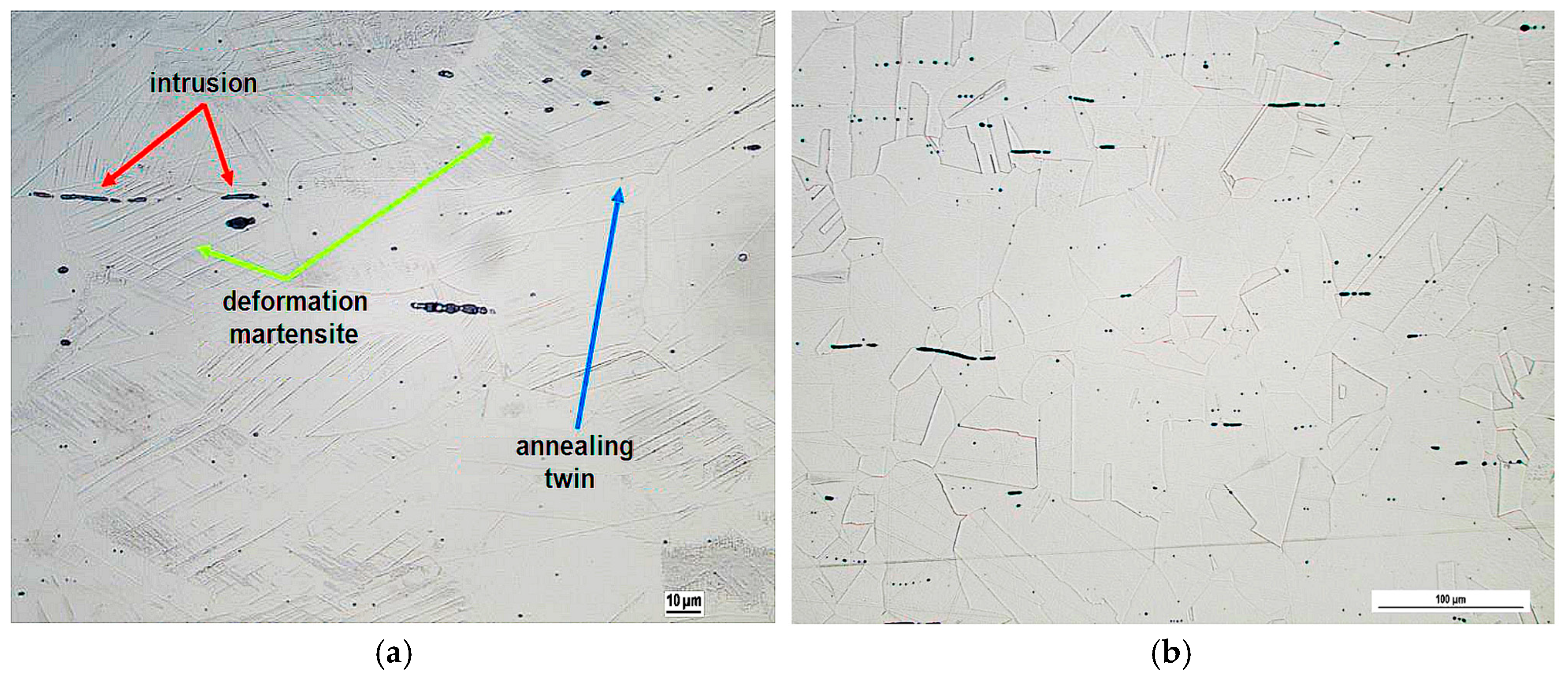
In the microstructure, there are numerous oval-shaped non-metallic intrusions of manganese sulfide (MnS), as shown in Figure 7a. The presence of sulfur in steel can be attributed to its occurrence in ores. Sulfur has a detrimental effect on austenitic steels, weakening their cohesion and leading to increased brittleness and decreased fatigue limit. However, the negative impact of sulfur can be mitigated by the presence of manganese, which binds to sulfur to form MnS. This binding process not only limits the degradative effects of sulfur but also increases the strength of the material.

At the same time, a relatively large number of typical annealing twins and deformation martensite with various orientations can be observed. These are formed due to plastic deformation, which involves cold rolling the bar in one direction to achieve the required square cross-section. It is important to note that heat treatment significantly alters the amount of deformation martensite. This leads to changes in the mechanical and magnetic properties of the material. This understanding is critical for assessing the behavior of austenitic steel at both microscopic and macroscopic levels. For better visualization, refer to Figure 7b, which shows a sample annealed at 1100 °C. The sample was then cut, manually sanded using P100 and P600 sanding wheels, and polished with diamond paste. After inducing the austenitic structure with an etchant, the resulting microstructure was observed using a microscope, as shown in Figure 7b. 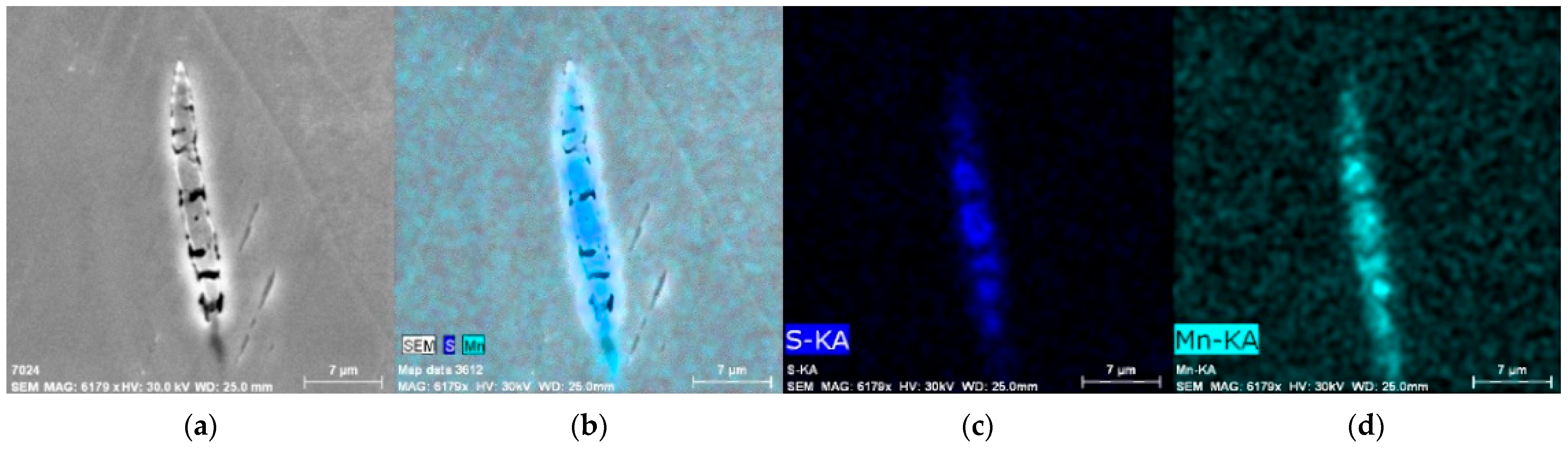By comparing images in Figure 6a,b and Figure 7a,b, there is a difference in the microstructure of the samples before and after annealing, specifically a decrease in the content of deformation martensite. The presence of sulfur in the composition was also confirmed through EDX analysis (Energy-Dispersive X-ray spectroscopy), shown in Figure 8, using a Scanning Electron Microscope (SEM). The non-metallic intrusion of manganese sulfide MnS is highlighted with blue, representing areas with sulfur and turquoise, indicating the presence of manganese.

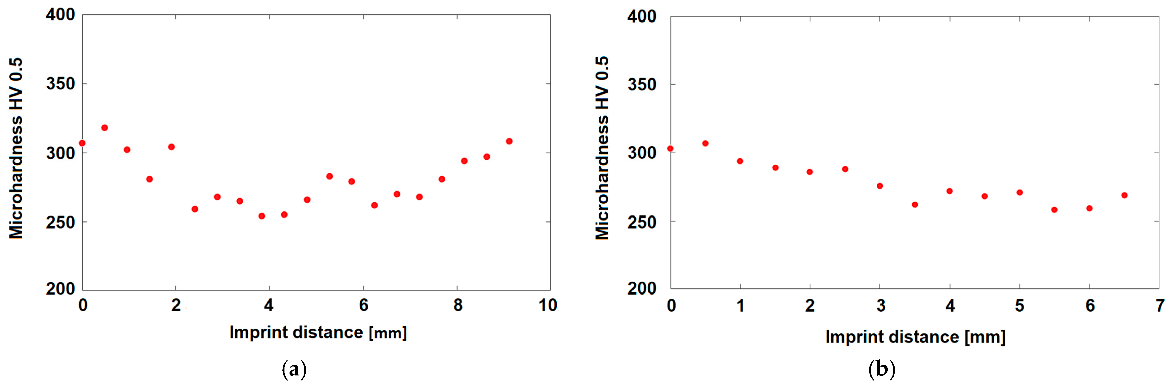
The initial state samples were measured for microhardness using a Zwick/Roell ZHµ microhardness meter on metallographically prepared samples. This method offers increased measurement accuracy due to the flat and polished surface and better visibility of impressions in the examined samples.

The measurement results in Figure 9a show the microhardness from the proximal part to the distal part of the sample. The figure illustrates that the course is relatively axisymmetric regarding the sample’s core. The arithmetic mean of microhardness in the longitudinal section was 281 HV 0.5, with a maximum value of 318 HV 0.5 and a minimum of 254 HV 0.5. In the second case, seen in Figure 9b, the identical sample was examined for its core, leading to an average value of 279 HV 0.5, with a minimum measured value of 258 HV 0.5 and a maximum of 307 HV 0.5. Based on the evaluation of the results, it can be concluded that the average microhardness value of the AISI 304 sample in the initial state is 280 HV at a load of 0.5 kg. The differences in microhardness depending on the measurement location are caused by several factors. The cold-rolled rod to prepare the samples led to plastic deformation, which modified the microhardness. Consequently, the core of the sample reached the lowest values, while the highest hardness was found at both ends of the sample. Additionally, microhardness values decrease as the indentation distance approaches the center due to the deformation’s impact, leading to the formation of deformation martensite with higher microhardness levels than the austenite grain itself. If the measuring diamond pyramid is in contact with the deformation martensite during the measurement, the microhardness reaches higher values.

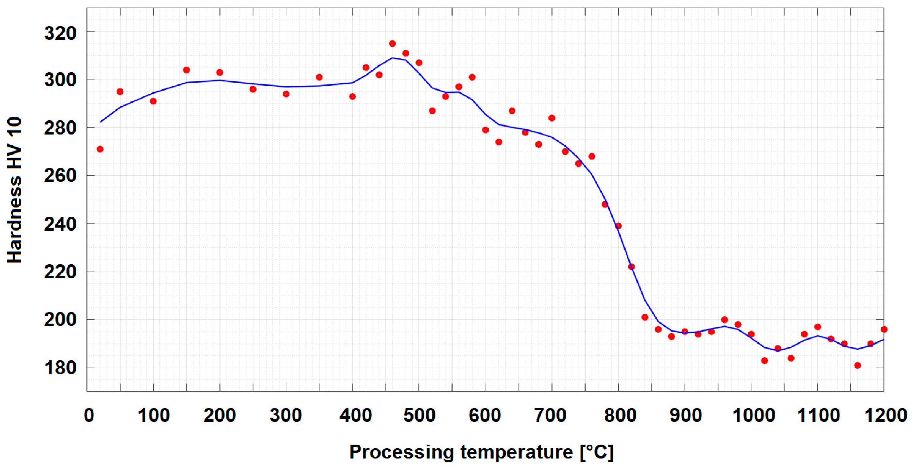
We made five measurements in each sample using a manual hardness tester and calculated the average hardness value. The results of these measurements at different annealing temperatures are displayed in Figure 10. The fluctuation of the obtained waveform can be caused by several factors (if we neglect the variability of the indenter and the measuring instrument). Possible causes include the following: the inhomogeneity of the microstructure, the presence of residual stresses and, of course, the history of the sample’s heat treatment. Surface roughness and sample preparation can also affect the obtained results, but in our case, the defined procedures were revised, and based on this, influence can be excluded.

Thanks to selecting different areas for measurements, implementing multiple measurements has eliminated measurement errors. Based on the results, the average hardness value of AISI 304 austenitic steel depends on the processing temperature. The hardness of the samples remains relatively consistent up to a temperature of 640 °C. Beyond this temperature, a gradual decrease in the hardness of the samples begins to be observed. The material’s hardness decreases significantly within the temperature range of 760 °C to 860 °C. This decrease is likely caused by the material’s recrystallization, resulting in reduced intrinsic stress and strain hardening. The gradual transformation of α’ martensite (deformation martensite) into austenite leads to changes in the material’s properties [25,26,27,28,29,30]. The material gradually softens and the structure reaches a state of equilibrium. The studied material acquires a constant value of hardness at approximately 860 °C. At this point, the process represents the annealing dissolution, and the samples attain a homogenized structure. In this range, several hardness values are the lowest within the entire hardness range.

Compared to the sample in its initial state, the average value after surpassing the annealing dissolution temperature decreased by approximately 100 HV 10. In comparing the hardness of the samples at the initial state and the sensitized findings, there was an increase in hardness. This increase in hardness in the sensitization temperature range, as shown in Figure 10, can be attributed to the precipitation of chromium carbide precipitates at the grain boundaries. These formed precipitates inhibit the movement of dislocations, which are the primary carriers of ductility and plastic deformation of the material. Chromium carbides also reduce defects in the crystal lattice of sensitized steels. Once the annealing dissolution temperature is reached, the hardness decreases due to the dissolved carbides formed as chromium enriches the matrix of the austenitic samples. If the annealing temperature was increased, the austenitic grains would further enlarge, reducing the samples’ hardness. This growth occurs only after the regeneration and recrystallization phase, per the knowledge presented in refs. [31,32,33,34,35]. The transformation of some parts of metastable austenite into deformation martensite due to plastic deformation increases the hardness, which is related to mechanical strengthening. The cold rolling process induces plastic deformation, significantly altering the properties of the steel due to increased dislocation density. Deformation can also initiate the sensitization process, during which the precipitation of chromium carbides can occur at the grain boundaries. Depleted areas may have a minimal deficiency in maintaining the material’s properties, leading to intracrystalline corrosion and subsequent artificial biocompatible implants.

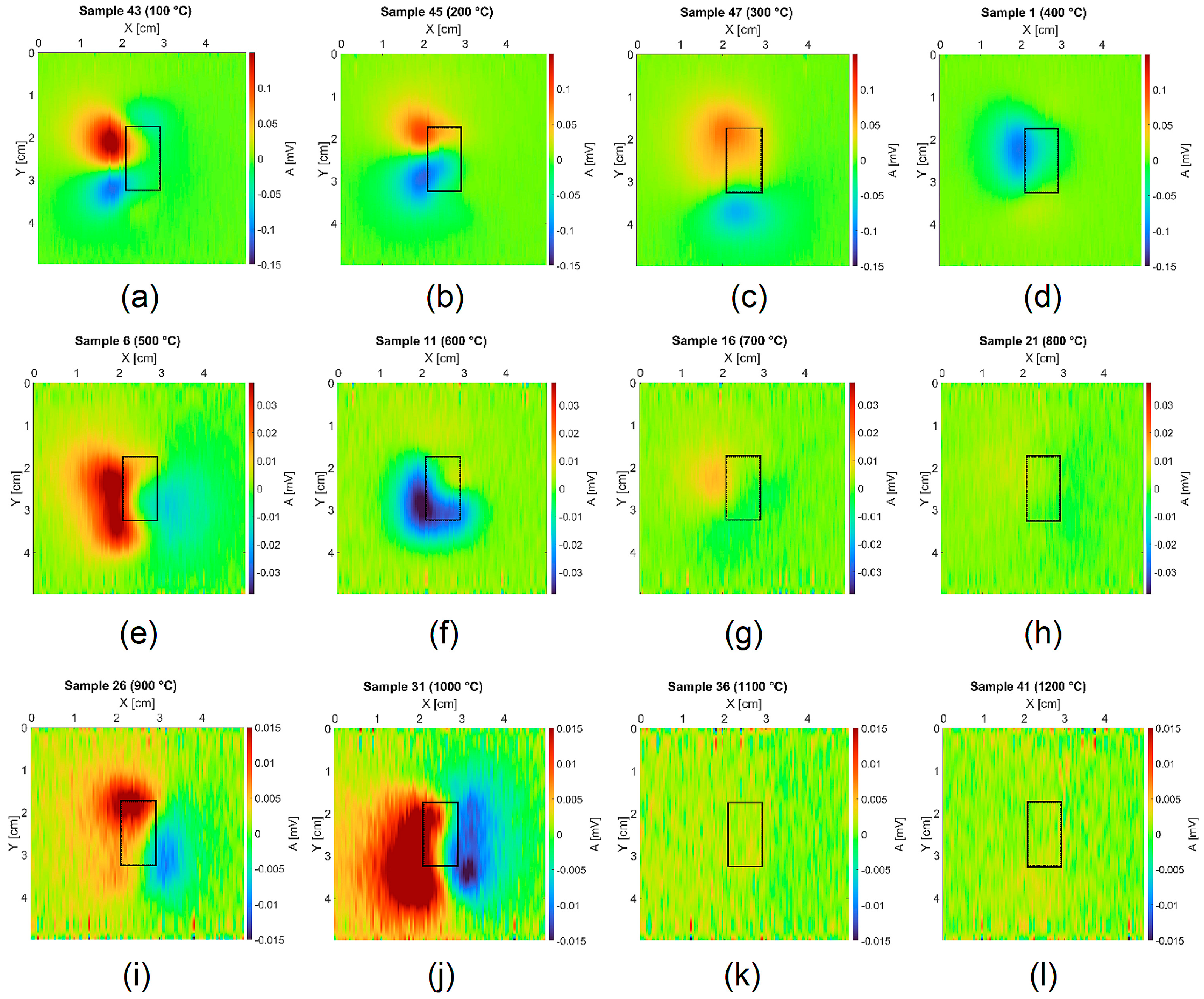
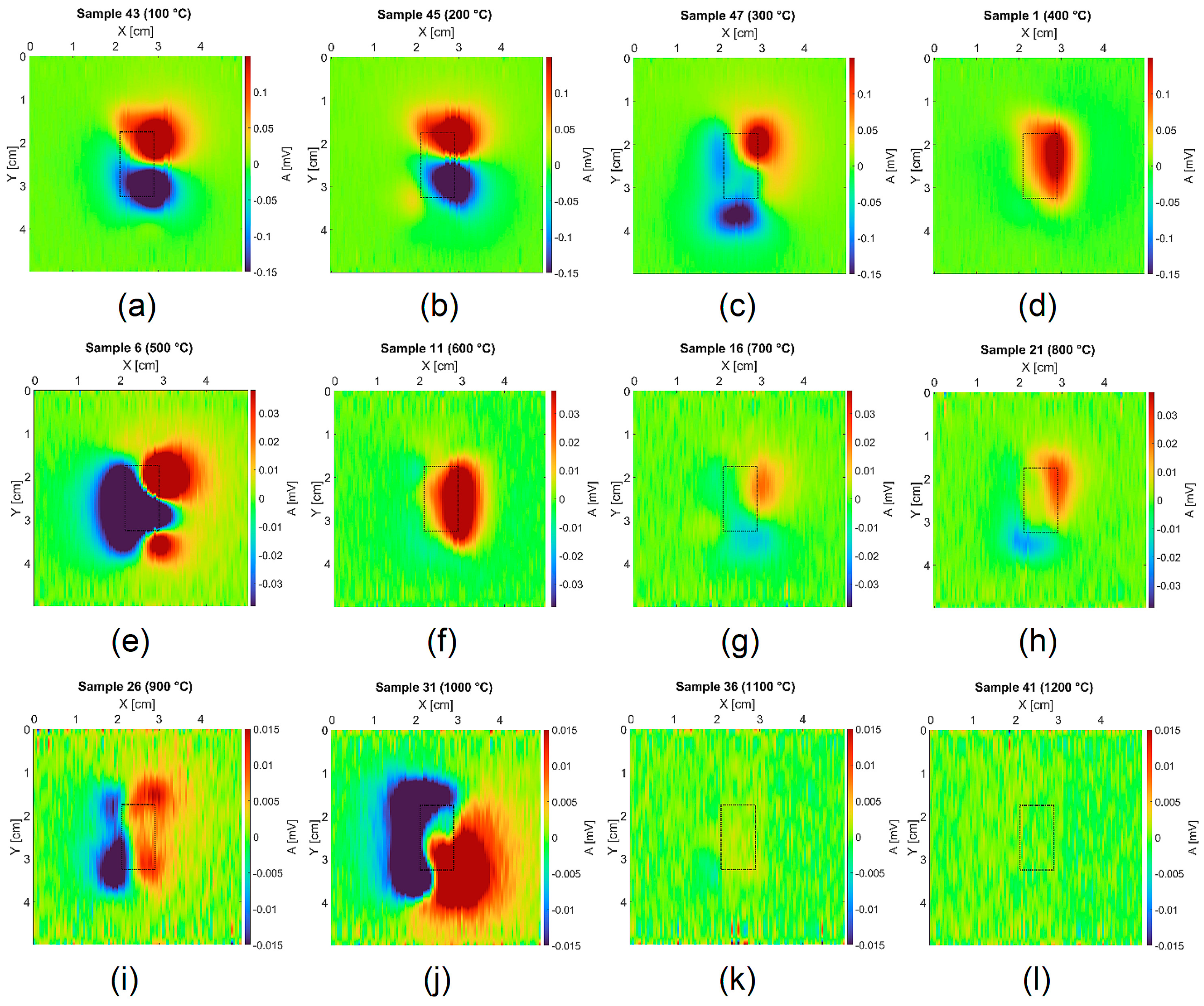
The measurement of magnetic properties was conducted using a reduced number of samples compared to the number used for measuring hardness. This reduction was implemented due to the less significant changes in magnetic properties among individual samples at temperature intervals of 25 °C. Measurements were consistently taken from two opposite sides of the samples, with neither side containing a numerical code. A stamped numerical code on the samples could negatively impact the measurement results due to additional plastic deformation near the code. It is crucial to measure magnetic properties from both sides of the samples, mainly when dealing with different orientations of the magnetic domains that can offset each other. A total of 13 samples were selected following a selection process, with annealing temperatures ranging from 50 °C to 1200 °C in increments of 100 °C. To verify the functionality and calibration of the measuring assembly, a sample annealed at 700 °C was specially molded for this purpose using Dentacryl and Bakelite, with the help of a Struers CitoPress-1 hot mounting device press. The magnetic field scan results are presented as a color-coded map with a 50 mm $\times$ 50 mm area, with the displayed quantity representing the DC electric voltage as a linear response of the fluxgate sensor to detect changes in the intensity of the magnetic field (refer to the calibration curve of the fluxgate sensor). The background noise of the magnetic field, part of any measurement, was suppressed by recording four signals over two consecutive days at the exact times of the sample measurements. A mean value was calculated from these reference measurements and then subtracted from all the measurements. This helped to partially eliminate the influence of artifacts such as electromagnetic interference from the surroundings, mainly due to the impact of various types of connections, and reduce the level of unwanted background noise. A script in the MATLAB R2024b software (MathWorks, Inc., Natick, MA, USA) was created to visualize the results in 2D maps.

Figure 11 and Figure 12 depict the detected intrinsic magnetic field of the samples in a graphical format. The intensity of the magnetic field is represented by colors on a specified scale, with the same values for positive and negative axes. The intrinsic magnetic field’s intensity scale is set to the same value for each row of figures. The maximum value is standardized for each row of graphs in the figures. Understanding the shape and distribution of the magnetic field in the samples is crucial for thoroughly analyzing the results. The quantity displayed is the DC voltage at the output of the fluxgate sensor, which demonstrates a linear response within the measurement range, as confirmed by its calibration curve.

Additionally, its axial sensitivity allows for the displayed quantity to be interpreted as an individual component of the magnetic field in 3D space (H_Z [A·m⁻¹]) from the perspective of the field’s shape. All the waveforms presented are shown as differential waveforms obtained through a method that eliminates artifacts caused by various sources of interference. It is important to consider that the sensor’s distance from the surface of the material being investigated significantly affects the quality of the obtained signals. As the distance increases, the sensor’s detection capability decreases sharply. The results presented set the distance at h = 1.5 mm. This article does not include results obtained from different distances (h = 2 mm, 4 mm, 8 mm, and 10 mm).

The individual graphs clearly show that the scanned field has a strong inhomogeneous character. When scanning from different sides of the sample, it is not possible to determine axial or central symmetry in the field. However, the material’s behavior at different annealing temperatures is evident from the characteristics. The phenomenon of a decrease in field intensity with increasing annealing temperature, or the sharp decrease and sudden increase at a temperature around T = 1000 °C, is noteworthy and deserves further investigation. It is also important to note that, from an overall perspective, the magnetic field of the samples creates a dipole moment, which depends on the processing conditions. Based on the results, this phenomenon can be observed where the dominant effect occurs in the narrow vicinity of T = 1000 °C and suddenly disappears.

The graph in Figure 13 illustrates how the intensity of the intrinsic magnetic field (measured as the output DC voltage of the fluxgate sensor) of all examined samples changes based on the annealing temperature. Each curve on the graph represents the intensity on the left and right sides of the sample, scanned separately. The third curve shows the average of the recorded responses.

Upon analyzing the results, it becomes evident that the intensity levels of the intrinsic magnetic field of the examined samples, as indicated by the sensor output signal values, are significantly influenced by the annealing temperature. The maximum intensity of the intrinsic magnetic field occurs when the sample is annealed at a temperature of T = 100 °C. Subsequently, the field intensity gradually decreases with increasing temperature. At specific temperature intervals, the intensity remains nearly constant. However, an increase is observed in the vicinity of the annealing temperature, T = 1000 °C, followed by a sharp decrease to almost zero. This points to a transition to the paramagnetic characteristic of the material structure at a macroscopic level.

For samples annealed at higher temperatures, magnetic properties significantly decrease. This decrease is likely attributed to the material’s recrystallization and the reduction of intrinsic stress. The gradual transformation of deformation martensite into austenite leads to alterations in the mechanical and magnetic properties of the analyzed samples. The magnetic property change can be attributed to deformation martensite exhibiting ferromagnetic properties, while austenite is paramagnetic.

It can be inferred that with an increasing annealing temperature, there is a gradual chaotic distribution of magnetic moments, eventually causing the substance to no longer exhibit extended ferromagnetic properties at a macroscopic level.

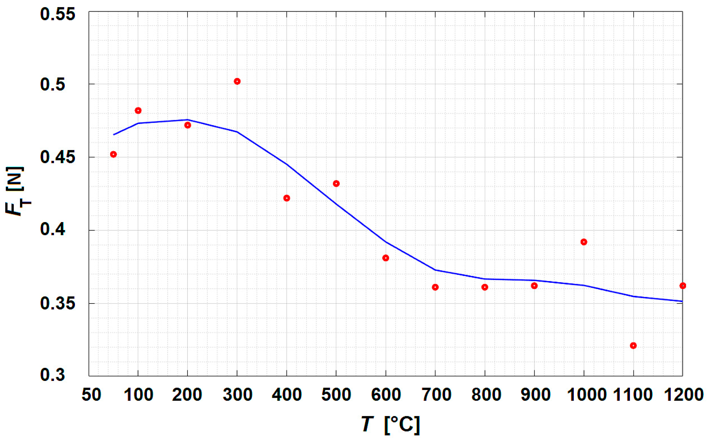
Three separate measurements were taken to determine the tear-off force for each sample. The average of these measurements was calculated to obtain the tear-off force value. Samples with higher tear-off force values also exhibited higher intrinsic magnetic field values. This means a greater force is needed to tear the sample from the permanent magnet.

Figure 14 illustrates the results of the tear-off force measurements of the heat treatment of the samples. The graph shows that the force required to tear off the magnet within the temperature range of 100 to 300 °C is higher compared to a temperature of 50 °C. As the annealing temperature exceeds 300 °C, the tear-off force gradually decreases. However, at annealing temperatures starting from 500 °C, this force stabilizes at approximately 0.37 N. The observed increase in this value at a temperature of 1000 °C correlates with the previously obtained results from the samples’ hardness and intrinsic magnetic field measurements.

4. Discussion

Analysis of the chemical composition revealed that the examined material did not meet the STN 17 240 standard for certain elements. An increased sulfur content, likely originating from the ore, weakened the cohesion of the austenitic grain, increasing brittleness and reducing toughness. The nickel content (7.8 wt %) was below the standard limit, potentially affecting corrosion resistance.

A microstructural analysis showed large polyhedral austenite grains, deformation martensite, and annealing twins. MnS inclusions were identified using EDX and an emission microscope. Microhardness measurements ranged from 254 to 318 HV 0.5, with lower values in the sample core and higher values at the edges. Hardness significantly decreased between 760 °C and 860 °C, with the lowest value (183 HV) measured at 1020 °C.

Magnetic field measurements with a fluxgate sensor indicated the highest intensity at 100 °C, gradually decreasing to 700 °C. A significant increase in magnetic field intensity at 100 °C suggests that deformation-induced martensite transformed into austenite in the 80 ÷ 100 °C range.

Tear-off force measurements revealed a gradual increase up to 500 °C, followed by a sharp decrease, stabilizing at 700 °C.

5. Conclusions

This study investigated electrically conductive biomaterials, focusing on AISI 304 austenitic stainless steel. The experiments included chemical and metallographic analysis, microhardness and hardness measurements, intrinsic magnetic field assessment, and tear-off force evaluation. These analyses provided essential insights into the material’s properties, which are critical for biocompatible implants and nondestructive inspections.

This research examined property changes in AISI 304 due to technological processes. Cold rolling induced plastic deformation, transforming austenite into deformation martensite (α’). Subsequent annealing at temperatures up to 1200 °C revealed that hardness increased after plastic deformation but significantly decreased above 760 °C. Magnetic field strength peaked at 100 °C and declined above 500 °C, correlating with the transformation of weakly ferromagnetic martensite into paramagnetic austenite.

These findings could help predict mechanical and electromagnetic changes in austenitic steels, particularly for implantable devices. Monitoring magnetic property variations could help detect damage early, preventing failures through timely interventions. This study’s insights may also support the design of devices for real-time damage detection in biomedical applications.