Abstract
Soil salinization is a significant threat to agricultural production, making accurate salinity prediction essential. This study addresses key challenges in the Yellow River Delta (YRD) soil salinity inversion, including (1) determining which Landsat 8 OLI level performs better, (2) identifying the most suitable month for salinity inversion, and (3) improving model performance and identifying important variables in modeling. Thus Landsat 8 OLI images (Level-1 and Level-2) for 12 months were collected, then images having less than 10% cloud cover were selected and processed to extract spectral values. A total of 86 sampled points were processed to measure soil salinity. Using Pearson correlation and expert insights, January 15 and August 26 were identified as suitable dates for inversion. Then, seven original bands, 29 spectral indicators, and 39 derived variables which created through six mathematical transformations, were used to construct the following three models: partial least squares regression (PLSR), random forest (RF), and backpropagation neural network (BPNN). The results showed the following: (1) The Level-1 data, after FLAASH atmospheric correction, outperforms Level-2 data. (2) January is optimal for salinity inversion. (3) Among the three models, RF outperformed the others, achieving test set R2 = 0.55, RMSE = 3.4, suggesting that the combination of spectral indicators and mathematically transformed variables can effectively enhance model accuracy for predicting soil salinity in the YRD. Furthermore, SWIR1, SWIR2, CLEX, second-order difference of SWIR1, and first-order difference of SWIR2 along with NIR played a key role in modeling.
1. Introduction
Soil salinization creates a significant threat to agricultural production and reduces the limited soil resources. Typically, it occurs in arid areas where the groundwater level is shallow while the salt content is elevated to the ground by the high evaporation, or it occurs in coastal areas affected by seawater erosion [1]. Climate, landscape, underground water, and many other factors may lead to soil salinization [2]. The Yellow River Delta is one of China’s most significant agricultural areas, facing severe soil salinization challenges, with many farmlands suffer from high level soil salinity [3], as a result of the two main factors of seawater erosion [4] and elevated salt content [5]. So, the monitoring and analyzing of soil salinity levels is crucial for sustainable agriculture. However, large-scale field monitoring is challenging and costly, making satellite imagery an economically viable alternative [6].
Since the 1960s, remote sensing technology has been widely employed to predict soil salinity due to its high spatiotemporal resolution, rapid data acquisition, and low cost [7]. Recent studies have quantitatively explored soil salinization by using various spectral indicators derived from remote sensing images [8]. Indicators such as the ratio vegetation index (RVI), modified soil adjusted vegetation index (MSAVI), normalized difference vegetation index (NDVI), normalized salinity index (NDSI), and salinity index (SI) have been employed to enhance prediction accuracy [9]. For example, Li et al. [10] combined various indicators to predict soil salinity in the Kenli county of the Yellow River Delta, finding that the normalized difference vegetation index (NDVI), ratio vegetation index (RVI), salinity index (SI3), and salinity index (SI5) can effectively enhance prediction accuracy. Zhang et al. [11] used the green difference vegetation index (GDVI), enhanced vegetation index (ENDVI), salinity index (SI-T), normalized difference water index (NDWI), and land surface temperature index (LST) to construct three models—BP neural network (BPNN), support vector machine (SVM), and random forest (RF)—for the inversion of soil salinity at different depths. Xu et al. [12] analyzed soil salinization in the Yellow River Delta from 2000 to 2020 using five indicators, as follows: modified soil adjusted vegetation index (MSAVI), salinity index (SI), kernel normalized difference vegetation index (KNDVI), three-band gradient difference vegetation index (TGDVI), and NDVI. In addition, scholars have also employed mathematically transformed methods to construct variables and reduce noise in the original data. For instance, Jiang et al. [13] employed mathematical transformations such as , , , , and first-order derivative while using light gradient boosting machine (LightGBM) for variable selection. They combined surface parameters to construct the sine–cosine algorithm (SCA) and deep extreme learning machine (DELM) models for soil salinity inversion. Kasim N et al. [14] constructed a partial least squares regression (PLSR) model to visualize salinization areas using first-order derivative , second-order derivative , , and first-order derivative . Wang et al. [15] used original band , , and continuous removal to build PLSR and SVM models, finding that the SVM performed better. These studies indicate that spectral indicators and mathematically transformed variables can be employed to construct soil salinity inversion models, thus optimizing model performance.
From the above text, it is evident that scholars have conducted extensive research on monitoring and predicting soil salinization using remote sensing technology. However, these articles still have room for improvement, as follows: (1) In terms of month selection, most of these articles chose remote sensing images close to the soil sample collection time without discussing which month is most suitable for inversion. (2) The impact of image levels has not been considered; most articles used Landsat 8 OLI Collection 2 Level-1 data as the data source while neglecting Level-2 data and have not compared the performance of the two types of data in soil salinity inversion. (3) Most authors chose either spectral indicators or mathematically transformed variables, without combining both data types, and the most suitable spectral variables are still not scientifically determined. Therefore, this study employed two levels of Landsat 8 OLI Collection 2 images: Level-1 and Level-2, 12 months; then, the images whose cloud cover was less than 10% were selected. Utilizing seven original bands, 29 different optical indicators, and derived 39 variables using six mathematical transformation methods (reciprocal , logarithm , exponential , square root , first derivative , and second derivative ) the three models of partial least squares regression (PLSR), random forest (RF), and backpropagation neural network (BPNN) were established. Finally, the following conclusions can be drawn: (1) which month is most suitable for inversion; (2) which level of Landsat 8 OLI Collection 2 performs better in model construction; (3) whether the combination of spectral indicators and mathematically transformed variables can improve model performance, and which variables are the most suitable for soil salinity identification.
2. Materials and Methods
2.1. Study Area
The study area is the Kenli county of the Yellow River Delta (latitude 37°24′–38°06′, longitude 118°14′–119°17′), located in Dongying City, Shandong Province, China, near the southern coast of Bohai Sea (Figure 1). This region has a warm temperate monsoon climate, with an average temperature ranging from 12.3 °C to 12.8 °C [16]. The area is flat, sloping from southwest to northeast, with an elevation between 1 and 13 m and a natural gradient of 1/8000 to 1/12,000. The shallow groundwater is highly saline. The soil is light-textured, generally lacking organic matter, nitrogen, and phosphorus, leading to poor nutrient conditions, with a pH greater than 7 [17]. The primary land-use types include cultivated land, unused land, and grassland, with main crops such as winter wheat, corn, rice, and cotton. White grass, reeds, horse trip grass, Tamarix, and Suaeda are the natural vegetation [18]. The variation in soil salinization is evident, making this an ideal area for study.
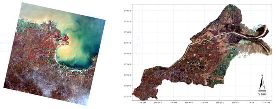
Figure 1.
Location of the study area and 86 sampling points. Red dots mean the sampled points. The data sources were Landsat 8 OLI Collection 2 Level-2 image taken on 15 January 2016 from the United States Geological Survey ©, https://earthexplorer.usgs.gov/ (accessed on 20 October 2024).
2.2. Ground Data
First, 96 sample points were designed. After field investigations, 86 samples were sampled in Kenli county, considering factors such as soil type, vegetation type, and land use. The sample area was set to 30 m × 30 m to match the pixel area of Landsat 8 OLI data, with a sampling depth of 0–20 cm, conducted from 11 October to 16 October 2016. All sampling points were located as far from roads and buildings as possible. The distance between adjacent sampling points was approximately 4.5 km, sufficient to avoid spatial dependence among samples. In this study, all georeferencing work was conducted using the U.S. Global Positioning System (GPS), with a handheld GPS device used to determine field coordinates and record surrounding environmental information. It is worth noting that in recent years, China’s BeiDou Navigation Satellite System (BDS) has been widely adopted for high-precision positioning and remote sensing applications in China due to its accuracy advantages. In future research, the adoption of BeiDou will be considered.
2.3. Laboratory Processing and Soil Salinity Measurement
The samples were processed and analyzed in the laboratory. First, the collected soil samples were air-dried, impurities were removed, and soil particles smaller than 2 mm were selected. Then, a soil solution was prepared using 20 g of soil sample and 100 mL of deionized water at a soil-to-water ratio of 5:1, from which the EC 1:5 value was extracted and measured using a conductivity meter. Subsequently, the soil samples were dried in an oven at 105° until a constant weight was reached, and the dry weight of the samples was measured to calculate salinity content and conductivity using our laboratory’s formula for soil salinity content and conductivity:
converting the EC value to soil salinity content (SSC) in g/kg. Descriptive statistics were conducted on the soil salinity data from the sampling points. Table 1 describes the average, standard deviation, range, minimum, maximum, and coefficient of variation (CV) for the samples. The results showed significant variation in soil salinity across the sampling area, ranging from 0.02 to 36.08 g/kg, with a CV of 176%, indicating that it nearly covered all salinity levels in the study area.

Table 1.
The statistical data of 86 samples. The statistical data unit is g/kg expect coefficient of variation.
2.4. Image Data Acquisition and Processing
Landsat 8 OLI Collection 2 Level-1 and Level-2 images were obtained from the US Geological Survey’s Earth Explorer platform (https://earthexplorer.usgs.gov/ accessed on 20 October 2024) for the year 2016.The images contain seven bands with a spatial resolution of 30 m, as detailed in Table 2.
Table 2.
Wavelength and resolution of 7 bands.
A total of 12 months of images were obtained, then those whose cloud cover was less than 10% were selected; these were the five months of January, February, March, August, and December. Since the August 10 image had higher cloud cover than August 26, the latter was retained. Landsat 8 OLI Collection2 images have two levels, Level-1 and Level-2, with the specific differences outlined in Table 3.
Table 3.
The difference between the two levels.
2.4.1. Processing of Landsat 8 OLI Collection 2 Level-1
Landsat 8 OLI Collection 2 Level-1 images required processing, including radiometric calibration and atmospheric correction, implemented in ENVI 5.6, with the FLAASH atmospheric correction [19]. The output images were converted from WGS 84/UTM zone 50N (EPSG: 32650) coordinate system to WGS 84 (EPSG: 4326). QGIS 3.34.0 software was used to extract spectral values from the processed images for the sample points. Finally, the soil reflectance for Landsat 8 OLI Collection 2 Level-1 was calculated by multiplying the extracted spectral values by scale factor 0.0001 (Table 3).
2.4.2. Processing of Landsat 8 OLI Collection 2 Level-2
The Landsat 8 Collection 2 Level-2 images did not require additional processing as they had already undergone atmospheric correction using surface reflectance code developed by Eric Vermote at NASA GSFC (LaSRC) [20]. Thus, the images from WGS 84/UTM zone 50N (EPSG: 32650) were converted to WGS 84 (EPSG: 4326) and then QGIS 3.34.0 was used to extract spectral values for the sample points. The soil reflectance for Landsat 8 OLI Collection 2 Level-2 was calculated by multiplying the extracted spectral values by scale factor 0.0000275 and then subtracting 0.2 (Table 3).
2.5. Data Selection
Images from five separate months were selected, as follows: January 15, February 16, March 3, August 26, and December 16, including both Level-1 and Level-2 data from Landsat 8 OLI, totaling 10 remote sensing images, as shown in Figure 2.
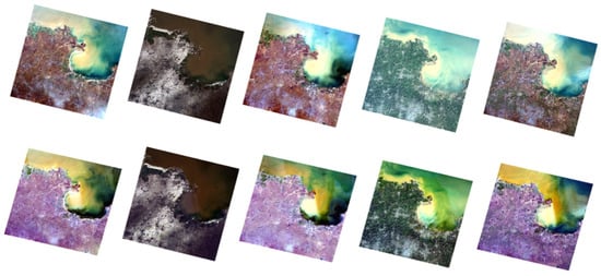
Figure 2.
The top images are Level-1, and the bottom images are Level-2. From left to right, the dates are January 15, February 16, March 3, August 26, and December 16. Different colors of images mean the different situation of ground.
Pearson correlation was applied to determine the relationship between salinity and spectral data for each month. The formula for Pearson correlation coefficient is expressed as follows:
This formula calculates the strength and direction of the linear relationship between two variables. The result ranges from −1 to 1, where represents the Pearson correlation coefficient with values near −1 indicating a negative correlation and those near 1 indicating a positive correlation; represents the -th value of variable represents the mean of represents the -th value of variable and represents the mean of .
2.6. Mathematical Transformation and Spectral Indicators Construction
The mathematical transformations used in this study include reciprocal , logarithm , exponential , square root , first derivative , and second derivative . The following formulas were used:
Reciprocal of spectral reflectance: = ;
Logarithm: ;
Exponent: ;
Square root: .
The differences between the adjacent elements was calculated, which is similar to performing a first-order difference on discrete data mathematically. The first-order difference of the discrete data points is represented as follows:
The second-order difference is obtained by performing another difference on the first-order difference, represented as follows:
Since a single band contains limited spectral information, after extracting the spectral reflectance from the remote sensing images, operations can be performed between different bands. These indicators are derived from prior calculations in existing research (see Table 4). A total of 29 common spectral indicators were selected.
Table 4.
Spectral indicators in this study B, G, R, NIR, SWIR1, and SWIR2 separately means band blue, green, red, near infrared, short wave infrared 1, and short wave infrared 2.
2.7. Feature Variable Selection for Model Construction
In the January 15 data, five points were removed due to the presence of NONE values in the spectral indicators “CRSI”. Similarly, in the August 26 data, one point was removed for the same reason. For the PLSR model, a Pearson correlation analysis, as discussed in Section 2.5, was conducted on the remaining points. In the January 15 data, 18 features with a correlation greater than 0.4 with soil salinity were selected, while 30 features with a correlation greater than 0.4 were chosen in the August 26 data. Since the random forest model is composed of multiple decision trees, it has a strong resistance to noise. Additionally, the BP neural network (BPNN), as a deep learning model, can automatically learn and select features. Therefore, all variables were used for these two models.
2.8. Inversion Model Construction, Accuracy Verification, and Salinity Visualization
First, the samples were sorted in ascending order of salinity. Then, one sample every four samples was selected to form a test set; the remaining samples were used to form a training set. The ratio of the training set to the test set was 3:1. During the model training, the training set was further divided into a training set and a validation set with a ratio of 4:1.
2.8.1. PLSR
Partial least squares regression (PLSR) is a statistical method used to model the linear relationship between two datasets, especially useful when both datasets contain multiple variables and multicollinearity exist among the variables. PLSR builds a model by extracting latent components from the two sets of variables (predictor set and response set, which can maximize the covariance structure between the predictors and responses. This method not only addresses the issue of multicollinearity among predictors but also allows for effective prediction when complex relationships exist between predictor matrix and response matrix ) [35]. The general multivariate basic equation is as follows:
where is the response matrix; is the modeling matrix; is the projection of , also known as the factor matrix; is the projection of ; and are orthogonal loading matrices; and and represent errors. Based on the estimated factors and and loading matrices and , a linear model between and can be established using the PLSR model. The equation is as follows:
where is the coefficient of the PLSR model, and is the error vector. This study explores the feasibility of establishing a quantitative relationship between soil salinity content and influencing factors using the PLSR model. In this study, GridSearchCV was used to tune the parameters for the PLSR model, searching for the number of principal components in the range of 0 to 10. Then, the model was trained using the optimal number of principal components.
2.8.2. RF
Random forest (RF) is an ensemble learning algorithm proposed by Breiman in 2001, combining classification trees [36]. This algorithm has advantages such as nonlinear mining capability, good noise resistance, strong adaptability to data distributions that do not meet any assumptions, and a fast training speed [37]. First, the RF model uses the bootstrap aggregating method to randomly draw n training subsets from the original training set. Then, K features (K < n) are randomly selected from each training set. In the next step, m sub-decision trees can be constructed from these K features, and their predictions are recalculated repeatedly. Finally, the model can vote on classification models and select the model with the most votes as the final decision [38]. The specific process is shown in Figure 3.
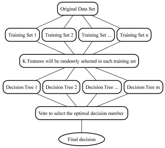
Figure 3.
RF flowchart.
For the RF regression task, for input sample, the regression result of the random forest is the average of the predictions from all trees:
where represents the prediction result of the -th tree for the input sample xxx; is the number of decision trees; and is the prediction result for the regression task.
In this study, GridSearchCV was used to search parameters for the random forest, searching for the number of trees by 10n (n being an integer, 5 ≤ ≤ 50), ranging from 50 to 500. The model was trained using the found number of trees.
2.8.3. BPNN
The back propagation neural network (BPNN) is one of the most fundamental and commonly used training algorithms in the field of deep learning [39]. The core of the backpropagation algorithm is based on the chain rule and gradient descent principle. During training, the network first performs forward propagation to compute the output result. Then, based on the error between the output and the expected output, backpropagation is used to calculate the contribution of each neuron’s weight and bias to the total error, and adjust the weights and biases to minimize the error function [40]. As shown in Figure 4, the neural network consists of input layers, hidden layers, and output layers, with each neuron represented by a node.
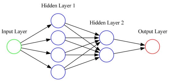
Figure 4.
BPNN flowchart.
The hidden portion can have one or more layers, with nodes from the previous layer connected to nodes in the next layer through weighted connections, forming a directed acyclic graph topology in the feedforward neural network structure. In the BP model, a nonlinear relationship between input and output can be achieved through linear combinations of inputs, as follows:
where is the unit input signal; is the number of neurons; is the unit output signal; is the connection weight between input unit i and output unit j; ξ is the bias; and f is the activation function of output unit .
In this study, the BP neural network (BPNN) was configured with a three-layer structure; the input layer had 75 nodes, the first hidden layer had 100 nodes, the second hidden layer had 50 nodes, and the output layer had 1 node. The activation function used was ReLu, with the optimizer being Adam, a learning rate of 0.001, and weight decay of 0.0001. The early stopping patience was set to 50, the dropout rate was 0.5, and the maximum training epochs were 2000, with a dropout proportion of 0.05. The loss function used was mean squared error (MSE).
2.8.4. Accuracy Verification
To verify the accuracy of the models developed in this study, 61 samples were used for model development and an independent validation dataset of 20 samples to assess the models’ performance. The evaluation metrics included root mean square error (RMSE), mean absolute error (MAE), standard deviation (SD), mean squared error (MSE), coefficient of determination (R2), with smaller values of RMSE, MAE, SD, and MSE indicating better model performance, while a larger R2 indicates better performance. The formulas for these five kinds of evaluation metrics are as follows [41]:
RMSE:
MAE:
SD:
MSE:
R2:
where is the predicted value; is the mean value; is the true value; and is the sample size.
2.8.5. Visualization of Salinity Distribution
Finally, we selected the best-performing model and the most suitable remote sensing images for salinity inversion to visualize the salinity distribution in the Yellow River Delta. The specific steps are as follows: 1. Load the remote sensing images and the best-performing model; 2. Use the model to predict the salinity values for each raster in the remote sensing image; 3. Classify the predicted results according to salinity levels and generate the salinity distribution map of the Yellow River Delta. And more details can be seen in Appendix A.
2.9. Methodology Workflow
This paper primarily describes the methods and experimental steps used to predict soil salinity in the Yellow River Delta. First, 86 points were sampled, and field coordinates were recorded. Then, EC values were measured in the laboratory and converted into salinity units (g/kg) using a specific formula. Next, Landsat 8 OLI Collection 2 data for 12 months were obtained, and the months with cloud cover below 10% were selected. The Level-1 data underwent radiometric calibration and atmospheric correction to extract spectral values, while Level-2 data were directly extracted. Afterward, Pearson correlation and expert insights were used to determine suitable dates for inversion. Spectral indicators and mathematical transformations were then calculated for the sampling points. Some points were removed due to “NONE” values in the “CRSI” indicator. The samples were sorted in ascending order of salinity. Then, every fourth sample was selected to form a test set, and the remaining samples were used to form a training set. Finally, models were built in Python 3.10. The precision of the three models was evaluated, and the salinity distribution was visualized using the best-performing model. The entire workflow is illustrated in Figure 5.
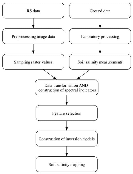
Figure 5.
Workflow of this research.
3. Results
3.1. Data Level and Month Selection
As shown in Table 5, in most cases, Level-1 data demonstrate stronger correlations between soil salinity and spectral data compared to Level-2 data. For instance, on January 15, the CO band in Level-1 data shows a correlation of 0.32 with salinity, significantly higher than 0.16 in Level-2. This trend, observed in March, August, and December data as well (with the exception of February 16), suggests that Level-1 data are more reliable in the CO band. Although the differences between Level-1 and Level-2 are relatively small in other bands, Level-1 data generally have slightly higher correlations overall. For example, on August 26, the B, G, R, SWIR1, and SWIR2 bands in Level-1 data all show slightly higher correlations. The only exception is the February 16 data, where Level-2 data exhibit marginally stronger correlations in the CO, B, G, R, and NIR bands. However, since the correlations on February 16 are generally low (all below 0.15), this date is excluded. Consequently, this study used the more strongly correlated Level-1 data for analysis.
Table 5.
The correlation between the seven bands and salinity.
When selecting an appropriate month for remote sensing of soil salinity, the following key factors were considered:
1. Correlation between Soil salinity and Spectral Bands. As shown in Table 5, data from January 15 and August 26 demonstrate significantly higher correlations between soil salinity and spectral data compared to other months. Specifically, on August 26, the CO, B, G, and R bands in Level-1 data all exhibit correlations above 0.4, with values of 0.32, 0.29, 0.27, and 0.21, respectively, while the corresponding bands in February, March, and December all fall below 0.2. From a correlation perspective, August 26 performs better than January 15.
2. Collinearity between Spectra bands. High collinearity may lead to information redundancy, which is unfavorable for building an accurate model. As Figure 6 indicates, on August 26, the CO band is highly correlated (above 0.7) with B, G, R, and SWIR2 bands. On January 15, while the CO band shows high correlation with B, G, and R, its correlation with SWIR1 and SWIR2 is very low. Additionally, on August 26, the B, G, and R bands also exhibit high correlation with SWIR2, while on January 15, B shows low correlation with SWIR2. The NIR and SWIR2 bands on January 15 show high correlation, while on August 26, the correlation is only −0.17. Finally, the total absolute sum of correlations between each band (excluding self-correlations) were calculated, with January 15 data totaling 11.57, lower than August 26’s 13.04, indicating lower collinearity in the January 15 data.
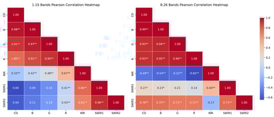
Figure 6.
The correlation of each band. * represents the p-value < 0.05 and ** represents the p-value < 0.01.
3. Expert and Literature Insights.
Consultations with agricultural remote sensing experts revealed that vegetation cover can interfere with the accuracy of salinity inversion, making it easier to observe salt accumulation during non-growing seasons. Additionally, Shao et al. [42] noted that soil salinity inversion may be influenced by air humidity. Humidity variations can affect the absorption and reflection of electromagnetic radiation, thereby impacting prediction stability. The Yellow River Delta is relatively dry in January, while August is more humid, suggesting January is better suited for salinity inversion.
In summary, although the August 26 data perform better in terms of correlation, the January 15 data are superior in terms of collinearity and the expert and literature support. Therefore, both January 15 and August 26 data were used to construct PLSR, RF, and BPNN models enabling the determination of the most suitable month for inversion.
3.2. The Result of Feature Variable Selection
For the PLSR model based on the January 15 data, a total of 18 variables were selected in the PLSR modeling (Table 6).
Table 6.
Correlation between soil salinity and the feature variables on the January 15.
For the PLSR model based on the August 26 data, the following 30 variables were selected in building PLSR modeling (Table 7).
Table 7.
Correlation between salinity and the feature variables on the August 26.
All 75 variables were used for the random forest (RF) and backpropagation neural network (BPNN) models, and were divided into the following three categories: 1. Original band data: CO, B, G, R, NIR, SWIR1, SWIR2 (seven variables). 2. Mathematical transformation variables, such as RECI_CO, LOGE_CO, EXP_CO, SQRT_CO, DIFF1B, DIFF2G, etc., (a total of 39 variables). 3. Spectral indicators (29 variables).
3.3. Optimal Model Parameter Results
For the PLSR model, the optimal number of principal components is 7 for the January 15 data and 10 for the August 26 data. For the RF model, the optimal number of decision trees is 140 for the January 15 data and 280 for the August 26 data. For the BPNN model, the optimal number of training epochs is 403 for the January 15 data and 455 for the August 26 data.
3.4. Accuracy Verification Results
The fitting performance of the three models is illustrated in Figure 7, Figure 8 and Figure 9, with five detailed evaluation metrics presented in Figure 10 and Figure 11. From Figure 7, it can be observed that the PLSR model performs better with the data from August 26 compared to January 15. Specifically, the test set R2 for January 15 is 0.25, while for August 26, it increases to 0.33. This improvement may be attributed to the PLSR model’s ability to better capture linear correlations, as indicated in Table 5, where the correlation on August 26 is higher than that on January 15. Figure 8 shows that the RF model demonstrates superior performance for January 15, with a test set R2 of 0.55, compared to 0.36 for August 26. Similarly, in Figure 9, the BPNN model also performs better with the January 15 data, achieving a test set R2 of 0.46, compared to 0.3 for August 26. From the detailed metrics in Figure 10, the RF model for January 15 exhibits the best performance, achieving a test set R2 of 0.55, RMSE of 3.4, MAE of 2.79, SD of 2.99, and MSE of 11.62, outperforming both the PLSR and BPNN models. In Figure 11, the RF model also performs the best for August 26, with a test set R2 of 0.36, RMSE of 5.6, MAE of 3.92, SD of 5.6, and MSE of 31.26.
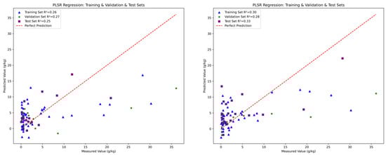
Figure 7.
The performance of PLSR for January 15 (left) and August 26 (right).
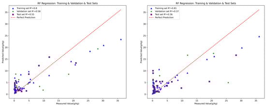
Figure 8.
The performance of RF for January 15 (left) and August 26 (right).
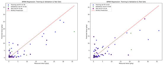
Figure 9.
The performance of BPNN for January 15 (left) and August 26 (right).
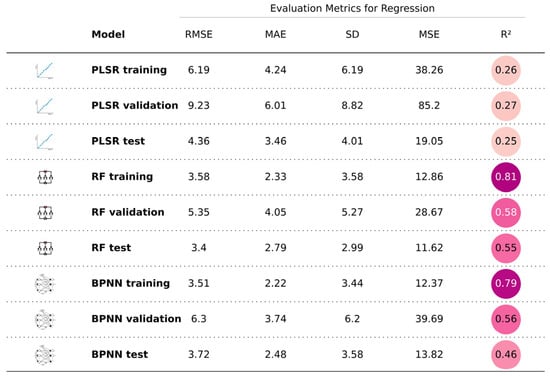
Figure 10.
Summary of the performance of the three models for January 15.
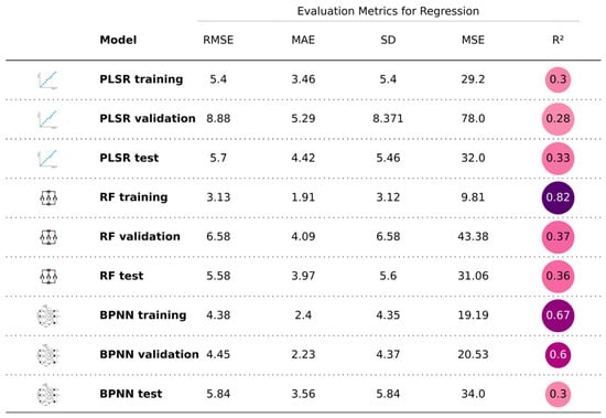
Figure 11.
Summary of the performance of the three models for August 26. The darker the color in the R2 area, the higher the R2 value; the lighter the color, the lower the R2 value.
In conclusion, the RF model for January 15 delivers the best overall performance, indicating that the data from January 15 are more suitable for salinity inversion. Furthermore, among the three models, the RF model consistently performs the best. This suggests that the random forest model can be used for soil salinity inversion in the Yellow River Delta. From Figure 10, it can be seen that both RF and BPNN performed well, with both models having an R2 greater than 0.45, indicating that using original spectra, spectral indicators, and mathematical transformation variables aids in model construction.
3.5. Visualization of Salinity Distribution in the Yellow River Delta
From the above results, it found that random forest performed the best in soil salinity inversion for the Yellow River Delta. Thus, the trained random forest model was applied to the atmospherically corrected Landsat 8 OLI Collection 2 Level-1 data from January 15 (already clipped into Kenli county according to the Shapefile). First, the image and the trained model were imported into Python. Then, applying the previously used data processing methods, including 29 indicators calculations and 6 data transformation methods (reciprocal , logarithm , exponential , square root , first derivative , and second derivative ), the random forest model utilized these data (original bands, spectral indicators, and mathematically transformed variables) to predict the salinity values of each raster, ultimately defining a color for each soil salinity level and creating a color map. The soil salinity distribution of the Yellow River Delta is shown in Figure 12.
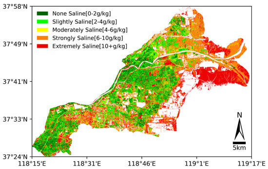
Figure 12.
Prediction of soil salinity in Yellow River Delta.
Additionally, the number of pixels for each color was obtained in python and then the surface area and the percentage of salinity for each class were calculated (Table 8).
Table 8.
The predicated area of soil salinity on each level.
To further elucidate the regional variations in soil salinity and the underlying geographical and hydrological driving factors, we introduced land use and soil classification data (see Figure 13). The land use map (a) shows land use data based on Sentinel-2 imagery with a 10 m resolution, while the soil classification map (b) is based on soil type data with a 1 km resolution. As shown in Figure 12 and Figure 13a, it is evident that our soil salinity inversion results highly align with the actual patterns.
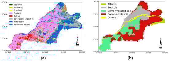
Figure 13.
(a) Sentinel-2 10 m resolution land use data are from https://viewer.esa-worldcover.org/worldcover/ (accessed on 28 October 2024) (b) Soil type classification is from the Natural Resources Network https://www.resdc.cn/data.aspx?DATAID=145 (accessed on 28 October 2024).
In terms of land use types, the distribution of non-saline and slightly saline areas largely overlaps with cropland. Specifically, non-saline areas occupy 16% (Table 8), a salinity level suitable for the growth of most plants, while slightly saline areas account for 23% (Table 8), a salinity level that only supports a few salt-tolerant plants. Therefore, at least 50% of the crops in the Yellow River Delta Kenli District are salt-tolerant crops such as cotton and wheat. On the other hand, cropland requires good irrigation conditions. From Figure 12, we can see that apart from the Yellow River flowing through the region, many lakes are distributed within the cropland, which also helps prevent the accumulation of soil salinity, thus reducing the degree of soil salinization. Additionally, as shown in Figure 12, areas of strongly and extremely saline are primarily concentrated near the coordinates 37°49′ N, 119°1′ E, close to the Yellow River mouth, where seawater intrusion significantly impacts the area. The moderately saline area often occurs alongside a strongly saline area. Table 8 shows that 12% of the soil is moderately saline while nearly 49% of the land is strongly saline or extremely saline, which is unsuitable for the growth of most plants. In Figure 13a, these areas correspond to herbaceous wetlands, water bodies, and bare/sparse vegetation areas. These observations further confirm that seawater intrusion increases soil salinity, making plant growth difficult. The overall salinity distribution of the region is also evident. Furthermore, we found that the salinity in built-up areas is particularly severe, possibly due to human activities leading to an excess of surface soil salts. There are very few trees planted in the built-up areas of the Kenli region, with most being grasslands, as shown in Figure 13a. Grasslands consume much less water compared to trees, which results in an imbalance in the water cycle. A large amount of water escapes the root zone and percolates down into the groundwater below. The construction of roads, buildings, and other infrastructures also alters the natural drainage pattern, and excess water may come from leaking sewage, rainfall, or water pipes. Over time, the underground water system fills up, bringing dissolved salts along with it. These salts accumulate beneath the surface, eventually leading to the formation of salinized areas. Urban salinization occurs due to the combined effects of excessive water and salt in the environment. Human activities significantly contribute to salinization.
In terms of soil type classification, as shown in Figure 13b, the strongly saline and extremely saline areas are predominantly found in saline–alkali soils, which are high in salts, strongly alkaline, and structurally poor, making them unsuitable for plant growth. Non-saline and slightly saline areas correspond to semi-hydrated soils and Entisols. Semi-hydrated soils contain higher moisture levels, though they typically do not reach saturation. The soil moisture is somewhat mobile, which helps dilute the soil salinity. Entisols are newly deposited soils, and as seen in Figure 13b, the flow of the Yellow River through this region keeps these soils in a dynamic state, where salts are either flushed away or dispersed by the water, thus maintaining non- or slightly saline status.
4. Discussion
4.1. Level and Month Selection
Landsat 8 OLI Collection 2 provides two levels of data, Level-1 and Level-2, so selecting the appropriate level is crucial. Both Level-1 and Level-2 data were downloaded, FLAASH atmospheric correction was performed on the Level-1 data, spectral values were extracted from both levels, and a Pearson correlation analysis was conducted between the extracted spectral values and salinity to select the appropriate level. Our study found that Level-1 data exhibited a higher correlation with salinity than Level-2 data. LaSRC is used to generate Landsat-8 OLI Level-2 surface reflectance data products. LaSRC utilizes auxiliary climate data from MODIS. Pinto et al. [43] found, through field measurements of surface reflectance, that the error prediction for Landsat-8 OLI Level-2 surface reflectance data showed significant discrepancies in the coastal aerosol band, with a notable decrease in consistency between coastal aerosols and the blue band. It was observed that aerosol extraction at certain sites may be unreliable. This finding aligns with our correlation analysis results, as the CO band of Level-1 data showed a higher correlation with salinity than the Level-2 band. The result indicates that Level-2 data are less reliable compared to Level-1 data.
Furthermore, since the effects of soil salinity inversion vary by month, selecting the appropriate month is crucial for accurate inversions. Salinity in the study area changes month by month, and as long as the internal patterns are understood, the timing of remote sensing imagery does not necessarily need to be confined to the sampling times. In selecting the month, three factors were considered, as follows: (1) the correlation between salinity and spectral bands, (2) the collinearity of the bands themselves, and (3) expert experience. The spectral values on August 26 had the highest correlation with salinity, while January 15 data showed lower collinearity. Expert experience and the literature suggest that January 15 data reduce the interference from vegetation and the low air humidity minimizes abnormal electromagnetic wave reflections, allowing for more effective salinity inversion. Thus, the data from August 26 and January 15 were used to build PLSR, RF, and BPNN models, and the month was selected based on the performance of the models. Ultimately, it found that the RF model built with January 15 data performed the best, with a test set R2 of 0.55, RMSE of 3.4, MAE of 2.79, SD of 2.99, and MSE of 11.62. In conclusion, January 15 data are more suitable for salinity inversion in the Yellow River Delta.
4.2. Feature Variables Selection, Model Construction, and Variable Contribution to the Model
Partial least squares regression (PLSR), random forest (RF), and backpropagation neural network (BPNN) were chosen as models for this study because these three represent different types. PLSR is a linear model, RF is a machine learning model, and BPNN is a deep learning model. The latter two models have considerable noise resistance.
Unlike previous studies, 29 spectral indicators were constructed and 6 mathematical transformation methods (reciprocal , logarithm , exponential , square root , first derivative , and second derivative ) were applied. For PLSR, variables selected through feature selection were used to build the soil salinity model, while for RF and BPNN, a total of 75 variables, including original bands, mathematically transformed variables, and spectral indicators were used. The results indicated that among the three models, RF performed the best, showing superior results in the training, validation, and test sets across five evaluation metrics, with the performance of the test set achieving an R2 of 0.55, RMSE of 3.4, MAE of 2.79, SD of 2.99, and MSE of 11.62. This shows that the RF algorithm effectively constructs the soil salinity inversion model.
Random forest is a nonlinear model capable of capturing nonlinear relationships. The final prediction is the average of the results from all decision trees, effectively reducing the impact of noise. Therefore, this study selected a total of 75 variables. However, it must be acknowledged that a large number of features increase the complexity of the model, prolong the training time, and consume more memory and CPU resources, which is particularly evident in the final visualization and unfriendly to low-performance computers.
Hence, we explored methods to further reduce the number of features and decrease model complexity. We obtained feature importance from the best-performing trained random forest model. In the random forest regression model, feature importance is calculated based on each feature’s contribution when constructing decision trees. This is determined by measuring the average reduction in mean square error contributed by each feature across all trees. After training the random forest model, the feature_importances attribute was used to extract the importance scores for each feature. According to the importance scores from the random forest, the top 20 most important variables for model construction were identified, as shown in Figure 14.
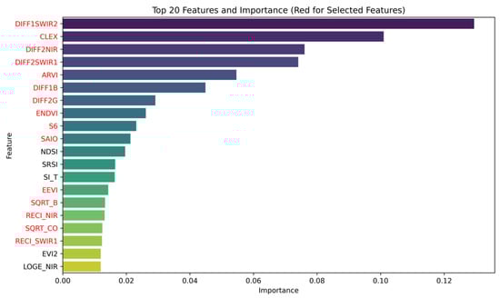
Figure 14.
Top 20 important variables in RF. The red words indicate variables retained after a correlation analysis in Figure 15, which filtered out variables with high correlation, then used to construct a new RF model.
Then, we built a new random forest model using the 15 features highlighted in red in Figure 14. These features were selected using Pearson correlation to eliminate those with collinearity above 97% (see Figure 15).
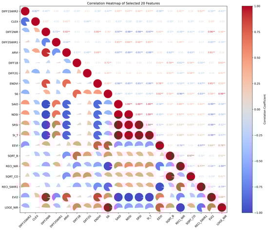
Figure 15.
The correlation heatmap of selected 20 features. * represents the p-value < 0.05 and ** represents the p-value < 0.01.
The results show that the random forest model built using 15 features achieved an R2 of 0.52 and an RMSE of 3.5 (see Figure 16) on the test set, compared to the model built with 75 features, which achieved an R2 of 0.55 and an RMSE of 3.4, indicating a slight decrease in performance. Therefore, it can be concluded that while random forest effectively captures nonlinear relationships and achieves relatively higher accuracy when using all 75 features, the model is more complex, requires longer training time, and consumes more CPU and memory resources. In comparison, the model built with the selected 15 features has slightly lower accuracy but is simpler, trains faster, and is more suitable for computers with lower performance.
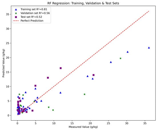
Figure 16.
The performance of RF constructed by 15 features.
Seen from Figure 14, CLEX’s formula is represented as follows:
While DIFF1SWIR2 is the first derivative of SWIR2, DIFF2SWIR1 is the second derivative of SWIR1. It can be observed that three of the top four variables are related to SWIR1 and SWIR2, suggesting that these bands play an important role in salinity inversion in the Yellow River Delta.
4.3. Comparisons with State-of-the-Art (SOTA), Other Models (This Study), and Performance, Across Different Months and Data Sets
4.3.1. Model Comparison with SOTA
In terms of model accuracy, the random forest (RF) model proposed in this study achieved an R2 of 0.55 on the test set for January 26, outperforming Jie’s SVR model (R2 = 0.4) [44] and Tiantian’s model (R2 = 0.5) on the validation set [45]. The RF model aggregates predictions from multiple decision trees, demonstrating stronger robustness. In contrast, linear models typically require manual feature selection and extensive data preprocessing. Deep learning models, while powerful, are highly sensitive to hyperparameter tuning, requiring adjustments to many parameters. The RF model, however, is less dependent on hyperparameters, requiring fewer settings and offering greater interpretability. Additionally, the feature importance plot in RF provides valuable insights into the key variables critical for model construction.
4.3.2. Comparison with This Study’s Other Models
The RF model outperforms the other models tested in this study. Specific performance metrics can be seen in Figure 10 and Figure 11.
(1) Data Distribution: Stratified sampling was applied to ensure that both the training and test sets maintained consistent distributions, representing a broad range of salinity samples. Thus, the differences in model performance are unlikely to be attributed to data distribution.
(2) Feature Importance: Both RF and BPNN models automatically select important features. On January 26, the RF model achieved an R2 of 0.55 and an RMSE of 3.4, whereas BPNN reached an R2 of 0.46 and an RMSE of 3.72. These results were significantly better than those of PLSR, which had an R2 of 0.25 and an RMSE of 4.36.
(3) Hyperparameter Settings: Hyperparameter tuning for the RF model is relatively simple, requiring only adjustments to the number of trees and leaf nodes. Future work will streamline this process by keeping the leaf node setting at its default value. In contrast, BPNN requires more complex hyperparameter tuning (e.g., learning rate, optimizer like Adam, number of layers), and is sensitive to these settings. Overfitting or underfitting is common during training, which may explain why the BPNN model performed poorly on August 26, with an R2 of only 0.3.
(4) Model Characteristics: PLSR is a linear model that assumes linear relationships between variables, which limits its performance in handling nonlinear problems. In August, the linear correlation between salinity and spectral data was stronger than in January, resulting in a higher R2 of 0.33 for PLSR in August compared to 0.25 in January. However, this study found that soil salinity inversion is not a simple linear problem. Both BPNN and RF, as nonlinear models, performed better in handling this complexity. Therefore, in January, RF achieved an R2 of 0.55 and an RMSE of 3.4, while BPNN had an R2 of 0.46 and RMSE of 3.72, outperforming PLSR (R2 = 0.25, RMSE = 4.36).
4.3.3. Random Forest Performance Across Different Months
RF demonstrated inconsistent performance between January and August, with an R2 of 0.55 in January and only 0.36 in August. Despite the similar sizes of the training and validation sets across the two months, and the consistent use of all variables in feature selection, several factors may explain the differences:
(1) Salinity and Spectral Correlation: In January, the correlation between salinity and spectral data was weaker than in August, but the collinearity issue was also less pronounced (as discussed in Section 3.1). This suggests that the information in the January dataset was more useful than in August. The summer month of August is characterized by lush vegetation, which could interfere with the accuracy of salinity inversion.
(2) Weather Conditions: The Yellow River Delta experiences dry conditions in January with little rainfall, whereas August is marked by higher humidity and rainfall. The increased moisture in the air during August can alter the way electromagnetic waves reflect and absorb, which may affect the accuracy of salinity inversion in the region.
4.3.4. Analysis of Performance Variations Across Training, Validation, and Test Sets
RF’s performance varied across the training, validation, and test sets, raising questions about the causes of this inconsistency, particularly in feature importance.
(1) Random forest: as an ensemble learning method, RF typically fits the training set well by constructing multiple decision trees and combining their predictions. This often leads to better performance on the training set than on the validation or test sets. For instance, the R2 for the training set on January 15 is 0.81, higher than 0.58 for the validation set and 0.55 for the test set. Similarly, on August 26, the R2 for the training set is 0.82, while the validation and test sets have R2 values of 0.37 and 0.36, respectively. This shows random forest’s tendency to fit the training data strongly. The similar performance of the validation and test sets suggests the model is reliable.
(2) Real-World Complexity: It is nearly inevitable that the training set will perform better than the validation and test sets. Salinity prediction is inherently challenging, and the model cannot capture all real-world data during training. The unpredictability of real-world scenarios means that new, unknown factors may arise during actual predictions, which is why training set performance often surpasses that of the validation and test sets (unless, as discussed later, independent test sets are not used, leading to overfitting or data leakage).
(3) Data Leakage Risk in Other Studies: Many studies rely on the performance of training and validation sets to draw conclusions, which can be unreliable due to potential data leakage, particularly in multi-round training. High R2 values in these sets may indicate overfitting rather than genuine model performance. This study mitigated this issue by introducing an independent test set, tuning hyperparameters based on the validation set performance, and verifying conclusions with the training set. The consistency between training and validation set performance further validated the reliability of the research findings.
4.4. Recommendations for Agricultural Producers and Environmental Policymakers
4.4.1. Recommendations for Agricultural Producers
(a) Based on Soil Salinity: Soil salinity can be divided into five levels according to its salinity (see Figure 12). For soil in different salinity levels, the planting areas should be reasonably allocated and the planting structure optimized according to soil type and crop salt tolerance: (1) Non-saline Areas: Suitable for growing staple crops such as wheat, corn, and rice. (2) Slightly saline Areas: Suitable for growing salt-tolerant crops such as soybeans and cotton. This area can support crops with relatively high salt tolerance but still requires proper water management and salt control. (3) Moderately Saline Areas: Suitable for planting high-quality forage crops such as alfalfa. Planting forage provides food for livestock while maximizing the utilization of saline–alkali land. (4) Strongly Saline Areas: Mainly suitable for planting halophyte economic crops, such as soda grass. These crops have strong adaptability to high-salinity environments and possess certain economic and ecological value. (5) Extremely Saline Areas: These areas have the most severe salinization and are generally not suitable for agricultural planting. However, wild plants such as reed and other halophytes can be considered for ecological restoration and wetland recovery.
(b). Technological Integration and Agricultural Management. To efficiently utilize saline–alkali land, in addition to the reasonable allocation of planting areas, it is necessary to strengthen technological integration and improve agricultural management: (1) Soil Improvement and Fertility Enhancement: Using organic fertilizers, green manure, and microbial fertilizers to improve soil structure, enhance soil fertility, and reduce salt accumulation. Methods such as adjusting soil pH and irrigation management can also be employed to effectively reduce the impact of salinity on crops. (2) Integration of Agricultural Machinery and Remote Sensing Technology: Combining advanced agricultural machinery, drones, and remote sensing technologies for precision farming. Remote sensing monitoring technologies can be used to dynamically track soil salinity and moisture conditions, enabling real-time monitoring of changes in water and salt content in saline–alkali land, and guiding precise fertilization and irrigation.
4.4.2. Recommendations for Environmental Policymakers
Establishing a Salinization Dynamic Monitoring Network: It is recommended that governments at all levels and local agricultural departments establish a comprehensive salinization monitoring network. Through the regular collection of remote sensing data and ground-based field data, they should comprehensively grasp the distribution and change trends of saline–alkali land resources. By monitoring the changes in saline–alkali land in real-time, corresponding mitigation measures can be taken in a timely manner to ensure the sustainable management of saline–alkali land.
4.5. Limitations of the Study and Future Plans
Compared to other studies, this research has certain limitations.
1. Temporal Resolution: The temporal resolution of Landsat 8 is relatively low, with images captured every 16 days, resulting in fewer available images compared to higher temporal resolution remote sensing data like Sentinel 2 [46]. Additionally, cloud cover further reduces the number of usable images. In 2016, there were only six images with cloud cover less than 10%. Therefore, the selected months in this study are limited to January, February, March, August, and December.
2. Lack of Consideration for Other Variables: combing the spectral information obtained from Landsat 8 with salinity to establish a soil salinity monitoring inversion model. However, only spectral information was used and did not incorporate other variables such as elevation, soil pH, and water content [47]. Water and salt are highly correlated during the process of soil salinization, and salinity can change with variations in water content. Thus, soil salinity is likely to vary with changes in moisture. In salinity monitoring, it is essential to consider both salinity and moisture to further develop coordinated monitoring of water and salt, achieving high monitoring precision and effectiveness. The next step is to use Sentinel 2 in conjunction with Sentinel 1 and more variable information for salinity inversion in the Yellow River Delta.
5. Conclusions
This study analyzes the use of Landsat 8 OLI remote sensing images for salinity inversion in the Yellow River Delta. The research area focuses on the Kenli county in Shandong Province, China. Two levels of Landsat 8 OLI Collection 2 data (Level-1 and Level-2) were downloaded, with the months having less than 10% cloud cover being January 15, February 16, March 3, August 26, and December 16. Pearson correlation analysis of the spectral values and field-sampled soil salinity was conducted to determine the most suitable data level and months for inversion. Then combining 29 spectral indicators and six data transformation methods (reciprocal , logarithm , exponential , square root , first derivative and second derivative ) and used original bands, spectral indicators, and transformed variables to construct the following three models: partial least squares regression (PLSR), random forest (RF), and back propagation neural network (BPNN). By constructing different models, the most suitable model was selected for salinity inversion in the Yellow River Delta to visualize the salinity distribution.
This study shows that the Level-1 data, corrected using FLAASH atmospheric correction, outperforms Level-2 data, with January being the most suitable month for salinity inversion among the selected months. The random forest model exhibited the best performance for salinity inversion in the Yellow River Delta, with training set. This indicates that the random forest model effectively reflects soil salinity.
Both the random forest (RF) and back propagation neural network (BPNN) models constructed in this study performed well, indicating that the construction of spectral indicators and mathematical transformations can effectively enhance the accuracy of soil salinity inversion in saline–alkali land. We also found that the original bands SWIR1 and SWIR2, along with their differentiated bands (second-order difference for SWIR1 and first-order difference for SWIR2), and the spectral indicators CLEX constructed from SWIR1 and SWIR2, play a significant role in the development of soil salinity inversion models. Additionally, the NIR band and its derived spectral index ARVI also demonstrate notable importance in the models. Overall, models constructed using original bands, spectral indicators, and transformed variables can provide better performance in soil salinity inversion and monitoring in the Yellow River Delta.
Author Contributions
Conceptualization, G.N. and Y.G.; methodology, X.Z.; software, G.N.; validation, G.N. and Y.G.; formal analysis, Y.G. and Y.L.; investigation, Z.R. and M.J.; resources, Y.Y.; data curation, X.Z.; writing—original draft preparation, G.N.; writing—review and editing, X.Z.; visualization, Y.G.; supervision, X.Z.; project administration, X.Z.; funding acquisition, X.Z. and X.L. All authors have read and agreed to the published version of the manuscript.
Funding
This research was supported by the Science & Technology Specific Projects in the Agricultural High-tech Industrial Demonstration Area of the Yellow River Delta, Grant No.: 2022SZX33. This project was also supported by the National Key Research and Development Program of China and Provincial student innovation plan project of Shandong, the Qingdao Agricultural Remote Sensing Application Engineering Research Center, Qingdao Agricultural University, Grant Nos.: 2021YFD1900902 and 2023YFD1902703.
Institutional Review Board Statement
Not applicable.
Informed Consent Statement
Not applicable.
Data Availability Statement
The data supporting the findings of this study are available at GitHub at the following link: https://github.com/woshiniguosheng/kenli_soil_salinity.git (accessed on 15 December 2024).
Acknowledgments
We would like to express our gratitude to the staff of The Comprehensive Utilization Service Center for Saline-Alkali Land in the Agricultural High-Tech Industry Demonstration Zone of the Yellow River Delta.
Conflicts of Interest
The authors would like to hereby certify that there are no conflicts of interest in the data collection, analyses, and interpretation, in the writing of the manuscript, and in the decision to publish the results.
Appendix A
| Algorithm A1: Summary pseudocode algorithm of this research. | |
| 1 | Algorithm: Soil Salinity Prediction |
| 2 | Input: |
| 3 | Spectral data from Landsat 8 OLI (band data) |
| 4 | Region of Interest (ROI) |
| 5 | Calibration data (soil salinity measurements) |
| 6 | Output: |
| 7 | Predicted soil salinity values |
| 8 | Visualized salt–alkali distribution map |
| 9 | |
| 10 | // Step 1: Data Preprocessing |
| 11 | Apply radiometric calibration and atmospheric correction to Landsat 8 OLI Level-1 |
| 12 | Apply scaling factors to Level-1 and Level-2 data |
| 13 | Extract band values (e.g., Band R) from the image data |
| 14 | |
| 15 | // Step 2: Data Transformation |
| 16 | For each band (B, G, R, NIR, SWIR1, SWIR2): |
| 17 | Perform mathematical transformations: |
| 18 | LOGE_Band = ln(Band) |
| 19 | RECI_Band = 1/Band |
| 20 | EXP_Band = exp(Band) |
| 21 | SQRT_Band = sqrt(Band) |
| 22 | DIFF1_Band = first difference of Band (along columns) |
| 23 | DIFF2_Band = second difference of Band (along columns) |
| 24 | Compute spectral indicators: |
| 25 | SI-T = R/NIR × 100 |
| 26 | NDVI = (NIR − R)/(NIR + R) |
| 27 | … (other spectral indicators) |
| 28 | Spectral_Variables = Original 7 bands + Transformed bands + Spectral indicators |
| 29 | |
| 30 | // Step 3: Feature Selection |
| 31 | PLSR_selected_features = [] |
| 32 | For each column in Spectral_Variables: |
| 33 | Calculate Pearson correlation between salinity and the column |
| 34 | If absolute correlation > 0.4: |
| 35 | Add column to PLSR_selected_features |
| 36 | |
| 37 | RF_selected_features = Spectral_Variables |
| 38 | BPNN_selected_features = Spectral_Variables |
| 39 | |
| 40 | // Step 4: Model Training and Evaluation |
| 41 | Split data into training (75%) and testing (25%) sets |
| 42 | |
| 43 | // PLSR |
| 44 | Create PLSR model |
| 45 | Define parameter grid for n_components (e.g., from 1 to 10) |
| 46 | Use grid search with cross-validation to find best PLSR model |
| 47 | For each n_components: |
| 48 | For each fold in cross-validation: |
| 49 | Train PLSR model on training data (of the current fold) |
| 50 | Calculate validation error (on the validation set of the current fold) |
| 51 | Select PLSR model with lowest average validation error across all folds |
| 52 | Calculate PLSR R-squared and other metrics on train, validation, test set |
| 53 | |
| 54 | // RF |
| 55 | Create random forest model |
| 56 | Define parameter grid for n_estimators (e.g., from 50 to 500) |
| 57 | Use grid search with cross-validation to find best RF model |
| 58 | For each n_estimators: |
| 59 | For each fold in cross-validation: |
| 60 | Train RF model on training data (of the current fold) |
| 61 | Calculate validation error (on the validation set of the current fold) |
| 62 | Select RF model with lowest average validation error across all folds |
| 63 | Calculate RF R-squared and other metrics on train, validation, test set |
| 64 | |
| 65 | // BPNN |
| 66 | Create BPNN model |
| 67 | Define network architecture (number of layers, activation functions) |
| 68 | Define training parameters (learning rate, batch size, number of epochs, optimizer) |
| 69 | Define a range of hyperparameters to tune (e.g., number of neurons, learning rate) |
| 70 | Use cross-validation to find the best BPNN model |
| 71 | For each combination of hyperparameters: |
| 72 | For each fold in cross-validation: |
| 73 | Train BPNN model on training data (of the current fold) |
| 74 | Evaluate BPNN model on validation data |
| 75 | Select BPNN model with best average performance on the validation set |
| 76 | Evaluate the best BPNN model: |
| 77 | Calculate BPNN R-squared and other metrics on train, validation, test set |
| 78 | |
| 79 | // Step 5: Visualization |
| 80 | Load best performing model (e.g., “model.pkl”) |
| 81 | Load Landsat 8 image (“image.tif”) |
| 82 | Calculate Bands, Spectral indicators, and Transformed variables in the Landsat 8 image |
| 83 | Predicting using the loaded model: Prediction_raster_values = model.predict(Data) |
| 84 | Soil_salinity_mapping = create_salinity_map(Prediction_raster_values) |
References
- Ruhollah, T.M.; Ayoubi, S.; Namazi, Z.; Malone, B.P.; Zolfaghari, A.A.; Sadrabadi, F.R. Prediction of soil surface salinity in arid region of central Iran using auxiliary variables and genetic programming. Arid Land Res. Manag. 2016, 30, 49–64. [Google Scholar]
- Guo, B.; Zang, W.Q.; Luo, W.; Wen, Y.; Yang, F.; Han, B.M. Detection model of soil salinization information in the Yellow River Delta based on feature space models with typical surface parameters derived from Landsat8 OLI image. Geomat. Nat. Hazards Risks 2020, 11, 288–300. [Google Scholar] [CrossRef]
- Chi, Y.; Sun, J.; Liu, W.; Wang, J.; Zhao, M. Mapping coastal wetland soil salinity in different seasons using an improved comprehensive land surface factor system. Ecol. Indic. 2019, 107, 105517. [Google Scholar] [CrossRef]
- Guan, B.; Yu, J.B.; Wu, M.D.; Liu, X.L.; Wang, X.H.; Yang, J.S.; Zhou, D.; Zhang, X.L. Clonal integration promotes the growth of Phragmites australis populations in saline wetlands of the Yellow River Delta. Front. Plant Sci. 2023, 14, 1162923. [Google Scholar] [CrossRef] [PubMed]
- Yu, C.X.; Wang, G.M.; Zhang, H.B.; Chen, H.P.; Ma, Q. Biochar and Nitrification Inhibitor (Dicyandiamide) Combination Had a Double-Win Effect on Saline-Alkali Soil Improvement and Soybean Production in the Yellow River Delta, China. Agronomy 2022, 12, 3154. [Google Scholar] [CrossRef]
- Wang, D.Y.; Chen, H.Y.; Wang, Z.R.; Ma, Y. Inversion of soil salinity according to different salinization grades using multi-source remote sensing. Geocarto Int. 2022, 37, 1274–1293. [Google Scholar] [CrossRef]
- Periasamy, S.; Ravi, K.P. A novel approach to quantify soil salinity by simulating the dielectric loss of SAR in three-dimensional density space. Remote Sens. Environ. 2020, 251, 112059. [Google Scholar] [CrossRef]
- Ma, Y.X.; Tashpolat, N. Current Status and Development Trend of Soil Salinity Monitoring Research in China. Sustainability 2023, 15, 5874. [Google Scholar] [CrossRef]
- Sahbeni, G.; Ngabire, M.; Musyimi, P.K.; Székely, B. Challenges and Opportunities in Remote Sensing for Soil Salinization Mapping and Monitoring: A Review. Remote Sens. 2023, 15, 2540. [Google Scholar] [CrossRef]
- Li, Y.S.; Chang, C.Y.; Wang, Z.R.; Zhao, G.X. Upscaling remote sensing inversion and dynamic monitoring of soil salinization in the Yellow River Delta, China. Ecol. Indic. 2023, 148, 110087. [Google Scholar] [CrossRef]
- Zhang, H.R.; Fu, X.; Zhang, Y.N.; Qi, Z.S.; Zhang, H.C.; Xu, Z.H. Mapping Multi-Depth Soil Salinity Using Remote Sensing-Enabled Machine Learning in the Yellow River Delta, China. Remote Sens. 2023, 15, 5640. [Google Scholar] [CrossRef]
- Xu, M.; Guo, B.; Zhang, R. A Novel Approach to Detecting the Salinization of the Yellow River Delta Using a Kernel Normalized Difference Vegetation Index and a Feature Space Model. Sustainability 2024, 16, 2560. [Google Scholar] [CrossRef]
- Jiang, X.F.; Duan, H.C.; Liao, J.; Guo, P.L.; Huang, C.H.; Xue, X. Estimation of Soil Salinization by Machine Learning Algorithms in Different Arid Regions of Northwest China. Remote Sens. 2022, 14, 347. [Google Scholar] [CrossRef]
- Kasim, N.; Maihemuti, B.; Sawut, R.; Abliz, A.; Dong, C.; Abdumutallip, M. Quantitative Estimation of Soil Salinization in an Arid Region of the Keriya Oasis Based on Multidimensional Modeling. Water 2020, 12, 880. [Google Scholar] [CrossRef]
- Wang, J.Y.; Li, X.M. Comparison on quantitative inversion of characteristic ions in salinized soils with hyperspectral based on support vector regression and partial least squares regression. Eur. J. Remote Sens. 2019, 53, 340–348. [Google Scholar] [CrossRef]
- Wang, J.J.; Wang, X.P.; Zhang, J.H.; Shang, X.D.; Chen, Y.Y.; Feng, Y.P.; Tian, B.B. Soil Salinity Inversion in Yellow River Delta by Regularized Extreme Learning Machine Based on ICOA. Remote Sens. 2024, 16, 1565. [Google Scholar] [CrossRef]
- Ouyang, Z.; Wang, H.; Lai, J.; Wang, C.; Liu, Z.; Sun, Z.; Hou, R. New Approach of High-quality Agricultural Development in the Yellow River Delta. Bull. Chin. Acad. Sci. 2022, 35, 145–153. [Google Scholar]
- Wu, Y.N.; Dai, L.Y.; Wang, Y.; Xie, L.M.; Zhao, S.Q.; Liu, Y.; Zhang, M.X.; Zhang, Z.M. Coexistence mechanisms of Tamarix chinensis and Suaeda salsa in the Yellow River Delta, China. Environ. Sci. Pollut. Res. 2020, 27, 26172–26181. [Google Scholar] [CrossRef]
- Wang, D.; Tang, B.H.; Li, Z.L. Evaluation of five atmospheric correction algorithms for multispectral remote sensing data over plateau lake. Ecol. Inform. 2024, 82, 102666. [Google Scholar] [CrossRef]
- Sayler, K. Landsat 8–9 Collection 2 (C2) Level 2 Science Product (L2SP) Guide; U.S. Geological Survey: Asheville, NC, USA, 2022; pp. 25–36.
- Tripathi, N.K.; Rai, B.K.; Dwivedi, P. Spatial modeling of soil alkalinity in GIS environment using IRS data. In Proceedings of the 18th Asian Conference on Remote Sensing, Kuala Lumpur, Malaysia, 20–24 October 1997; pp. 81–86. [Google Scholar]
- Khan, N.M.; Rastoskuev, V.V.; Sato, Y.; Shiozawa, S. Assessment of hydrosaline land degradation by using a simple approach of remote sensing indicators. Agric. Water Manag. 2005, 77, 96–109. [Google Scholar] [CrossRef]
- Allbed, A.; Kumar, L.; Aldakheel, Y.Y. Assessing soil salinity using soil salinity and vegetation indicators derived from IKONOS high spatial resolution imageries: Applications in a date palm dominated region. Geoderma 2014, 30, 1–8. [Google Scholar] [CrossRef]
- Taghizadeh-Mehrjardi, R.; Minasny, B.; Sarmadian, F.; Malone, B. Digital mapping of soil salinity in Ardakan region, central Iran. Geoderma 2014, 213, 15–28. [Google Scholar] [CrossRef]
- Chen, J.M. Evaluation of vegetation indicators and modified simple ratio for boreal applications. Can. J. Remote Sens. 1996, 22, 229–242. [Google Scholar] [CrossRef]
- Broge, N.H.; Leblanc, E. Comparing prediction power and stability of broadband and hyperspectral vegetation indicators for estimation of green leaf area index and canopy chlorophyll density. Remote Sens. Environ. 2001, 76, 156–172. [Google Scholar] [CrossRef]
- Liu, H.Q.; Huete, A.R. A feedback based modification of the NDVI to minimize canopy background and atmospheric noise. IEEE Trans. Geosci. Remote Sens. 1995, 33, 457–467. [Google Scholar] [CrossRef]
- Jiang, Z.; Huete, A.R.; Chen, J.; Chen, Y.; Li, J.; Yan, G.; Zhang, X. Analysis of NDVI and scaled difference vegetation index retrievals of vegetation fraction. Remote Sens. Environ. 2006, 101, 366–378. [Google Scholar] [CrossRef]
- Qi, J.; Chehbouni, A.; Huete, A.R.; Kerr, Y.H.; Sorooshian, S. A modified soil adjusted vegetation index. Remote Sens. Environ. 1994, 48, 119–126. [Google Scholar] [CrossRef]
- Wu, W.; Mhaimeed, A.S.; Al-Shafie, W.M.; Ziadat, F.; Dhehibi, B.; Nangia, V.; De Pauw, E. Mapping soil salinity changes using remote sensing in Central Iraq. Geoderma Reg. 2014, 2, 21–31. [Google Scholar] [CrossRef]
- Jiang, H.; Ding, J.; Tashpolat, T.; Zhao, R.; Zhang, F. Extracting salinized soil information in arid areas using ETM+ data. Acta Pedol. Sin. 2008, 45, 222–228. [Google Scholar]
- Chen, H.; Zhao, G.; Chen, J.; Wang, R.; Gao, M. Remote sensing inversion of saline soil salinity based on modified vegetation index in estuary area of Yellow River. Trans. Chin. Soc. Agric. Eng. 2015, 31, 107–114. [Google Scholar]
- Bannari, A.; Morin, D.; Bonn, F.; Huete, A.R. A review of vegetation indicators. Remote Sens. Rev. 1995, 13, 95–120. [Google Scholar] [CrossRef]
- Alhammad, M.S.; Glenn, E.P. Detecting date palm trees health and vegetation greenness change on the eastern coast of the United Arab Emirates using SAVI. Int. J. Remote Sens. 2008, 29, 1745–1765. [Google Scholar] [CrossRef]
- Ramole, A.; Skidmore, A.K.; Cho, M.A.; Mathieu, R.; Heitkonig, I.M.A.; Dudeni-Tlhone, N.; Schlerf, M.; Prins, H.H.T. Non-linear partial least square regression increases the estimation accuracy of grass nitrogen and phosphorus using in situ hyperspectral and environmental data. ISPRS J. Photogramm. Remote Sens. 2013, 82, 27–40. [Google Scholar] [CrossRef]
- Breiman, L. Random Forests. Mach. Learn. 2001, 45, 5–32. [Google Scholar] [CrossRef]
- Loozen, Y.; Rebel, K.T.; de Jong, S.M.; Lu, M.; Ollinger, S.V.; Whelan, M. In Situ Measurements and Remotely Sensed Retrievals of Soil Salinity in Coastal Wetlands: A Review. Remote Sens. 2020, 12, 4595. [Google Scholar]
- Hoa, P.V.; Giang, N.V.; Binh, N.A.; Hai, L.V.H.; Pham, T.D.; Hasanlou, M.; Bui, D.T. Soil salinity mapping using SAR Sentinel-1 data and advanced machine learning algorithms: A case study at Ben Tre Province of the Mekong River Delta (Vietnam). Remote Sens. 2019, 11, 128. [Google Scholar] [CrossRef]
- Wang, X.; Zhang, F.; Ding, J.; Kung, H.T.; Latif, A.; Johnson, V.C. Estimation of soil salt content (SSC) in the Ebinur Lake Wetland National Nature Reserve (ELWNNR), Northwest China, based on a Bootstrap-BP neural network model and optimal spectral indicators. Sci. Total Environ. 2018, 615, 918–930. [Google Scholar] [CrossRef]
- Rumelhart, D.E.; Hinton, G.E.; Williams, R.J. Learning representations by backpropagating errors. Nature. 1986, 323, 533–536. [Google Scholar] [CrossRef]
- Chicco, D.; Warrens, M.J.; Jurman, G. The coefficient of determination R-squared is more informative than SMAPE, MAE, MAPE, MSE and RMSE in regression analysis evaluation. PeerJ Comput. Sci. 2021, 7, e623. [Google Scholar] [CrossRef]
- Golestani, M.; Chahfarokhi, Z.M.; Esfandiarpour-Boroujeni, I.; Shirani, H. Evaluating the spatiotemporal variations of soil salinity in Sirjan Playa, Iran using Sentinel-2A and Landsat-8 OLI imagery. Catena 2023, 231, 107375. [Google Scholar] [CrossRef]
- Pinto, C.T.; Jing, X.; Leigh, L. Evaluation Analysis of Landsat Level-1 and Level-2 Data Products Using In Situ Measurements. Remote Sens. 2020, 12, 2597. [Google Scholar] [CrossRef]
- Jie, L.; Tingting, Z.; Yun, S.; Zhengshan, J. Comparing Machine Learning Algorithms for Soil Salinity Mapping Using Topographic Factors and Sentinel-1/2 Data: A Case Study in the Yellow River Delta of China. Remote Sens. 2023, 15, 2332. [Google Scholar]
- Cheng, T.; Zhang, J.; Zhang, S.; Bai, Y.; Wang, J.; Li, S.; Javid, T.; Meng, X.; Sharma, T.P.P. Monitoring soil salinization and its spatiotemporal variation at different depths across the Yellow River Delta based on remote sensing data with multi-parameter optimization. Environ. Sci. Pollut. Res. 2022, 29, 24269–24285. [Google Scholar] [CrossRef] [PubMed]
- Gorji, T.; Yildirim, A.; Hamzehpour, N.; Tanik, A.; Sertel, E. Soil salinity analysis of Urmia Lake Basin using Landsat-8 OLI and Sentinel-2A based spectral indicators and electrical conductivity measurements. Ecol. Indic. 2020, 112, 106173. [Google Scholar] [CrossRef]
- Yu, H.; Liu, M.Y.; Du, B.J.; Wang, Z.M.; Hu, L.J.; Zhang, B. Mapping Soil Salinity/Sodicity by using Landsat OLI Imagery and PLSR Algorithm over Semiarid West Jilin Province, China. Sensors 2018, 18, 1048. [Google Scholar] [CrossRef]
Disclaimer/Publisher’s Note: The statements, opinions and data contained in all publications are solely those of the individual author(s) and contributor(s) and not of MDPI and/or the editor(s). MDPI and/or the editor(s) disclaim responsibility for any injury to people or property resulting from any ideas, methods, instructions or products referred to in the content. |
© 2025 by the authors. Licensee MDPI, Basel, Switzerland. This article is an open access article distributed under the terms and conditions of the Creative Commons Attribution (CC BY) license (https://creativecommons.org/licenses/by/4.0/).