Field Strength Prediction in High-Speed Train Carriages Using a Multi-Neural Network Ensemble Model with Optimized Output Weights

Abstract

Accurate path loss prediction within train carriages is crucial for deploying base stations along high-speed railway lines. The field strength at receiving points inside carriages is influenced by outdoor signal transmission, penetration through window glass, and multiple reflections within the carriage, making it challenging for traditional models to predict the field strength distribution accurately. To address this issue, this paper proposes a machine learning-based path loss prediction method that incorporates ensemble techniques of multiple neural networks to enhance prediction stability and accuracy. The Whale Optimization Algorithm (WOA) is used to optimize the output weight configuration of each neural network in the ensemble model, thereby significantly improving the overall model performance. Specifically, on the test set, the WOA-optimized ensemble model reduces RMSE by 1.47 dB for CI, 0.47 dB for CNN, 0.93 dB for RNN, 1.38 dB for GNN, 0.1 dB for Transformer, 0.09 dB for AutoML, 0.33 dB for the GA-optimized ensemble model, and 0.18 dB for the PSO-optimized ensemble model.

1. Introduction

The fifth generation of mobile communication technology (5G) ensures the high-speed railway (HSR) system can provide high-quality, high-rate communication service [1,2,3,4,5]. Therefore, researchers have proposed various modeling approaches for the signal propagation characteristics of high-speed railways to improve the accuracy and practicality of path loss prediction.

1.1. Traditional and Neural Network Approaches

The deterministic channel modeling approach, primarily based on ray-tracing (RT) methods [6,7], has been widely used due to its high accuracy. For example, in [8], a two-path propagation model was validated using RT simulations to analyze the impact of Brewster’s angle on path loss. On the other hand, geometry-based stochastic channel models (GBSM) [9,10,11,12] offer greater flexibility and computational efficiency. For instance, Ref. [13] proposed a GBSM model for high-speed railway viaducts, analyzing the impact of scatterer distribution on channel characteristics. However, despite their advantages, RT methods become computationally expensive and complex when multiple factors in high-speed rail carriages are considered. At the same time, GBSM models, though efficient, often sacrifice accuracy and struggle to capture the detailed characteristics of specific environments.

Recent studies have explored the potential of artificial intelligence (AI) in predictive channel modeling [14,15,16,17,18,19,20,21,22,23]. Various neural network architectures have been applied to improve path loss prediction and channel estimation accuracy. For instance, Ref. [15] utilized a backpropagation neural network (BPNN) to predict path loss in aircraft cabins, achieving superior accuracy compared to the classical log-distance model. Similarly, Ref. [16] employed feedforward and radial basis function neural networks (FNN and RBFNN) for predicting received power and channel characteristics in indoor millimeter-wave channels.

Recurrent neural networks (RNNs) and long short-term memory (LSTM) models have been widely used for dynamic channel prediction. Ref. [17] applied an RNN to predict signal amplitudes and channel impulse response (CIR) in MIMO channels, removing the need for prior channel knowledge. Building on this, Ref. [18] introduced an online training LSTM model to predict channel state information (CSI) and improve performance by continuously updating the model. In high-speed scenarios, Ref. [20] proposed a real-time CNN-based channel prediction model that adapted dynamically to changing conditions, outperforming traditional methods.

Convolutional neural networks (CNNs) have also been combined with other techniques, such as in [19], where CNNs were integrated with 5G channel models to enhance estimation accuracy in MIMO-OFDM systems, and in [20], where CNNs were used for real-time channel prediction in high-speed environments. Ref. [21] conducted a comparative study of various neural network architectures, including CNNs, RNNs, and multilayer perceptrons, for wireless channel prediction, providing valuable insights for model selection.

Additionally, Ref. [22] introduced a federated learning-based approach for mmWave massive MIMO systems, combining RNNs with collaborative learning, which proved effective in non-stationary environments. Finally, Ref. [23] proposed a hybrid method combining graph neural networks (GNNs) with the propagation graph technique to model complex channel relationships, achieving superior results in irregular topologies.

Despite these advancements, these studies highlight the limitations of single-model approaches. Challenges such as limited generalization across diverse channel conditions and reduced predictive accuracy in highly complex scenarios remain critical issues to be addressed.

1.2. Ensemble Learning Approaches

Ensemble learning, a technique that integrates the strengths of multiple models, has emerged in recent years as a key approach to addressing the limitations of single models [24,25]. Combining the predictions of multiple base learners, ensemble learning not only enhances the generalization ability of models but also effectively reduces the bias and variance of individual model predictions, thereby achieving higher prediction accuracy and stability. Common ensemble methods, including Bagging [26,27], Boosting [28,29], Stacking [30,31], and Voting [32,33], offer different strategies for combining base learners, each contributing to improved model performance in various applications. In the complex scenario of channel prediction, ensemble learning has demonstrated significant potential due to its ability to integrate multi-source data features, improve model robustness, and enhance noise resistance. Research indicates that ensemble learning has been widely applied in channel prediction tasks.

For instance, random forest has shown strong performance in path loss prediction tasks due to its low computational complexity and good prediction accuracy [34]. Nonetheless, its relatively simple model structure may struggle to capture the nonlinear characteristics of complex channel environments. Particularly in intricate propagation scenarios such as high-speed train carriages, the random forest’s limited ability to handle the interaction of multiple influencing factors can lead to reduced prediction accuracy. The study in [35] systematically evaluated the performance of ensemble methods such as voting, bagging, and gradient-boosting trees for predicting path loss in rural environments. Ultimately, a stacking ensemble method combining five different base learners was adopted, achieving significant improvements in prediction performance. That said, the stacking approach employed a three-layer neural network, whose high model complexity may result in prolonged training times and overfitting.

In [36], the authors proposed an artificial neural network based on double-weighted neurons (DWN-ANN). The proposed model exhibited satisfactory alignment between prediction outcomes and measured data, outperforming traditional empirical models. Nevertheless, as it employs a sequential integration strategy, it may face challenges related to local optima. The layer-by-layer training and updating approach might not fully exploit the global information within the data and could reduce computational efficiency. In [37], the authors trained multiple neural networks with varying hyperparameters to enhance model diversity and combined their predictions to obtain the final results. Yet, the study did not provide an in-depth analysis of the output weights of each neural network, which could affect the optimization of the ensemble results.

1.3. Proposed Solution and Contributions

In conclusion, existing studies provide valuable insights into path loss prediction and channel modeling but have limitations in areas such as optimizing neural network configurations, determining the number of networks in ensemble models, and allocating output weights. Traditional models, like ray-tracing and geometry-based stochastic models, are inefficient and costly in high-speed train environments, limiting their accuracy and generalization. While advanced neural network methods like CNN and RNN show potential, they struggle with the complex channel characteristics in high-speed train carriages. CNNs are good at feature extraction but unstable in dynamic environments, while RNNs are strong at capturing temporal features but have limited generalization in noisy conditions. Moreover, ensemble learning methods still face challenges, such as choosing the optimal number of networks and efficiently allocating output weights, limiting their performance in path loss prediction.

To overcome these challenges, the research presented in this paper proposes a multi-neural network ensemble approach for path loss prediction in high-speed train carriages. Optimizing output weight configurations is carried out to improve accuracy and stability. Performance comparisons with traditional and advanced neural network methods will demonstrate the advantages of our approach. The primary contributions of this paper are as follows:

• A channel measurement campaign at 2.6 GHz was conducted in a high-speed train environment. Based on the measurement data, an RT model was calibrated. The calibrated RT model can generate large-scale, authentic, and reliable channel datasets.
• The performance of neural networks with varying numbers of hidden layer neurons was evaluated to address the complexity of channel modeling in high-speed train compartments. A candidate set of neural networks was constructed, and progressive integration methods were applied to optimize the overall prediction performance. Subsequently, progressive screening was employed to identify the optimal combination of neural networks for optimizing the overall prediction.
• To tackle the challenge of optimizing the output weights of base learners in ensemble learning, the whale optimization algorithm was introduced. By adaptively adjusting the output weights of each base learner, the prediction accuracy and robustness of the ensemble model were significantly improved.
• The experimental results show that, compared with other methods, the proposed model achieves substantial improvements in root mean square error (RMSE), mean absolute error (MAE), mean absolute percentage error (MAPE), and coefficient of determination R², thereby validating its effectiveness and practicality.

The following section outlines the structure of the remainder of this paper. Section 2 presents the communication scenario of high-speed rail signals penetrating train carriages and outlines constructing a high-precision dataset. Section 3 elaborates on the overall framework of the field strength prediction method for high-speed train carriages and the multi-neural network ensemble approach. Section 4 evaluates and compares the performance of the multi-neural network ensemble model with traditional and advanced neural network methods using the prediction dataset. Section 5 successfully summarizes the study’s findings and outlines future work.

2. Channel Measurement and Simulation

This section examines wireless channel characteristics in high-speed rail environments to optimize communication performance. A two-path model is developed, considering direct and reflected transmission and window penetration loss. Channel measurements at 2.6 GHz are conducted inside the train, with the data used to calibrate a ray-tracing (RT) simulation. The accuracy of the RT model is validated through comparisons of theoretical calculations, measurement results, and simulation data. Finally, large-scale simulations generate a high-precision path loss dataset across various seat positions and heights, supporting wireless communication optimization in HSR scenarios.

2.1. Communication Scenario

Figure 1 depicts a representative communication model between a high-speed rail base station (BS) and a mobile station (MS) within the train carriage. In this model, the projection of the base station onto the xoy plane is set as the coordinate origin. The vertical distance from the base station to the railway track is defined as the station-track distance D, d represents the Euclidean distance between the transmitting and receiving antennas, $h_T$ is the height of the transmit antenna, and $h_R$ is the height of the receive antenna. The communication link between the high-speed rail base station and the train terminal involves multiple paths. These include the direct line-of-sight path from the base station to the train terminal, the reflection path inside the carriage, and the ground reflection path. All signal paths traverse the high-speed rail carriage windows.

2.2. Two-Path Theoretical Model

Based on the two-path communication model for HSR proposed in [8], the field strength equation for the signal arriving at the seat in a two-path communication scenario can be derived. The two-path model assumes that there are two paths for the signal: one is the direct path, and the other is the path reflected through the ground or obstacles. In this scenario, the expression for the received power can be expressed as:

$$\begin{array}{c}Pr=Pt+20n{log}_{10}\left(\left({\displaystyle \frac{\lambda }{4\pi d}}\right)\times \left|1+R_{//}{e}^{jk{r}^{\prime }}+(1-R_{//})R_{//}{e}^{jk{r}^{″}}\right|\right)\\ +G_r+G_t-L\left({\theta }_{LOS}\right)-L\left({\theta }_R\right)\end{array}$$

(1)

where $Pt$ is the known to transmit power, n is the path loss exponent, $G_t$ is the directional gain of the transmit antenna, and $G_r$ is the directional gain of the receive antenna; d is the distance between the transmitting and receiving antennas; $r^{\prime }$ is the length of the reflection path; $r^{″}$ is the length of the reflection path in the presence of a second reflection length; $k=2\pi /\lambda$ is the wave number; $\lambda$ is the wavelength; $R_{//}$ is the Fresnel reflection coefficient under parallel polarization with the following equation:

$$R_{//}={\displaystyle \frac{\frac{\epsilon 2}{\epsilon 1}cos{\theta }_i-\sqrt{\frac{\epsilon 2}{\epsilon 1}-{sin}^2{\theta }_i}}{\frac{\epsilon 2}{\epsilon 1}cos{\theta }_i+\sqrt{\frac{\epsilon 2}{\epsilon 1}-{sin}^2{\theta }_i}}}$$

(2)

where $\theta i$ is the reflection angle of the ground, $\epsilon 1$ is the dielectric constant of air, and $\epsilon 2$ is the dielectric constant of the ground. In addition, the penetration losses of the direct and reflected diameters in the HSR glass are expressed by $L\left({\theta }_{LOS}\right)$ and $L\left({\theta }_R\right)$, respectively; $\theta$ is the angle of the signal incident on the glass and the HSR glass penetration loss formula $L\left(\theta \right)$ is derived based on the measured data of the HSR compartment glass penetration loss [8], which is given by the following equation:

$$L\left(\theta \right)=-0.0001\times {\theta }^3+0.0111\times {\theta }^2-0.6903\times \theta +31.3069$$

(3)

As shown in Figure 2, the direct and reflected diameter HSR glass incidence angle formula can be calculated separately for the angles when the direct and reflected diameters are incident on the glass under the seats of different compartments. Then, the angle of incidence ${\theta }_{LOS}$ of the direct path transmission into the glass is:

$${\theta }_{LOS}=arctan({\displaystyle \frac{h_T-h_R}{d_y}})$$

(4)

The angle of incidence ${\theta }_R$ of the reflection path transmission into the glass is:

$${\theta }_R={\displaystyle \frac{\pi }{2}}-arctan({\displaystyle \frac{d_y}{h_T+h_R}})$$

(5)

2.3. Channel Measurement

Measurements were conducted in the second-class passenger carriage of the Fuxing CR400BF train at 2.6 GHz using vertically polarized omnidirectional fiberglass antennas. The test scenario is illustrated in Figure 3. The transmitter, placed at the junction of Carriages 1 and 2 at a height of 3.6 m, emitted continuous-wave signals, while the receiver was positioned at the carriage center, flush with the glass, at 2.6 m.

To balance accuracy and efficiency, measurement intervals varied: starting from the center of the carriage, aligned with the transmitting antenna, measurements were taken every 1 m for the first 10 m; from 10 to 22 m, measurements were taken every 2 m due to signal stability; from 23 to 31 m, the interval returned to 1 m due to increased signal fluctuations; and from 31 to 50 m, measurements were taken every 2 m to ensure systematic coverage. In total, 34 measurement points were strategically planned to capture comprehensive signal data.

Measurement variability was considered, with fluctuations mainly caused by environmental factors such as wind, temperature, humidity, and electromagnetic interference. To minimize errors, tests were conducted under stable weather conditions using a fixed transmitter setup. For each measurement point, ten measurements were taken within one minute, and the average value was recorded to reduce random errors and enhance reliability.

Prior to data collection, extensive equipment calibration was performed. The field strength tester was compared against a high-precision standard field strength source across a range of values relevant to HSR environments. Multiple measurements were taken, analyzed using the least squares method, and used to generate a calibration curve for error correction. Similar calibration procedures were applied to the signal source and antennas, ensuring measurement accuracy and reliability.

2.4. Ray-Tracing Simulation

The ray-tracing simulation can calibrate material property parameters such as relative permittivity, conductivity, and roughness based on the received power data from actual measurements. This paper uses Wireless Insite’s ray-tracing simulation tool to simulate the HSR seat path loss. Based on the measured scenario and the 3D train model, the wireless channel simulation model in the HSR plain scenario is built, as shown in Figure 4. In the simulation scenario, there are four carriages; the transmitter antenna is located at the center of the connection between Carriage 1 and Carriage 2, the antenna height is 3.6 m, and the distance between the station rails is 5 m. The measured data calibrates the wireless channel model constructed.

Figure 5 illustrates the received power values obtained through the ray-tracing method after several adjustments to the material property parameters, compared with both the measured results and theoretical values. The path loss results from the simulation closely align with the measured data, demonstrating the high accuracy and reliability of our ray-tracing model. To further highlight the consistency between the simulation and measurement data, we present the following comparison in

Table 1. Statistical comparison of received power data between simulation and measurement.

Method	Mean (dBm)	Standard Deviation (dB)	K-S
Measurement	−77.96	8.25	0.7406
Simulation	−79.48	9.11

. This table provides a detailed statistical comparison of key parameters between the simulated and actual measured received power data. The mean difference between the measured and simulated data is 1.52 dB, the standard deviation difference is 0.86 dB, and the K-S test value is 0.7406, all of which indicate a high level of consistency between the two data. The optimized material parameters for the compartments are provided in

Table 2. Material properties after calibration.

Name	Material	Relative Permittivity	Conductivity (S/m)	Roughness
Track	Metal	∞	-	0
Carriage	Metal	∞	-	0
Luggage rack	Glass	6.27	0.0134	0
Wooden doors	Wood	1.99	0.0131	0.03
Seats	Textiles	3.03	11	0.01

.

Based on the calibrated model, further simulations were conducted to obtain a high-precision data set of path loss for the seats in the high-speed train carriage. The distance between the transmitting antenna and the train tracks (D) is 100 m, with the transmitting antenna placed at a height of 25 m, aligned with the x-axis coordinates of the first row of seats in the first carriage. The train consists of 8 carriages, and the frequency is 2.6 GHz. As shown in Figure 6a, the receiving antennas are omnidirectional, with six spatial sampling points arranged in each row of seats. The aisle position is labeled as E, and the seat positions are labeled as ABCDF, following the train’s seat numbering system. Above each seat and aisle position, five receiving antennas with different heights (I, II, III, IV, V) are installed at heights of 2.376 m, 2.476 m, 2.576 m, 2.676 m, and 2.776 m, respectively, to reflect the typical usage scenarios of high-speed train passengers. Position A refers to the antenna on the side farthest from the transmitting antenna, while position F refers to the antenna closest to the transmitting antenna. Figure 6b shows that the receiving antennas are placed in rows 1 to 18 of the carriage seats, excluding connections such as through-paths between adjacent carriages. A total of 4320 receiving points were established, creating a high-precision data set with 4320 samples through simulation.

3. Prediction Method

This section presents the field strength prediction method for high-speed train carriages based on the channel simulation dataset. The structure of this method forms the basis for model development, prediction, and optimization. In this subsection, we outline the key steps, including model structure, output weight optimization using the Whale Optimization Algorithm, and final prediction, providing a clear roadmap for the in-depth analysis that follows.

3.1. Overall Structure

Figure 7 illustrates the method used in this paper to predict field strength in high-speed train carriages. The dataset is divided into three subsets: the training set, the validation set, and the test set. The training set is used to train multiple models, the validation set is used to evaluate base models and optimize ensemble weights using the WOA, and the test set is used for final model evaluation to assess generalization on unseen data. In the neural network selection phase, networks with different hidden layer configurations are trained, and the top 10 performing models are selected. These models are then integrated step by step from one to ten networks. The ensemble consists of R neural networks, and the best combination is chosen by comparing the performance of different configurations. The WOA is used to optimize the integrated model’s output weights, balancing each sub-model’s contributions. Finally, the test set is input into the optimized model to generate predictions, which are verified by comparing them with the test data.

3.2. Multi-Neural Network Ensemble Model

The multi-neural network integration model has multiple BPNNs, with multiple fully connected layers as hidden layers; each input neuron is connected to each output neuron. A hyperparameter optimization process was performed to construct the optimal integration structure. The hyperparameters considered include the number of hidden layers, the number of neurons in each hidden layer, and the type of activation function. The training data set was used to train each artificial neural network during the network training process. The validation set is used to detect and prevent overfitting.

BPNN systematically solves the problem of learning the connection rights of hidden layers in multilayer networks by the gradient descent method, where the input variables are fed from the input layer and processed by the hidden layer to reach the output layer. The error between the output and actual values is calculated, and the error information is fed back to the network through backpropagation. We use the gradient descent method to repeatedly adjust the connection weights and thresholds between layers until the global error of the network is minimized so that the network output approximates the actual output. The path loss prediction results for a single BPNN model can be expressed as follows:

$$P{L}_{BPNN}=F_{BPNN}\left(R_s,C_s,C,d,{\Delta }_x,{\Delta }_y,h_R|w,b,\sigma \left(·\right)\right)$$

(6)

where $R_s$, $C_s$, C, d, ${\Delta }_x$, ${\Delta }_y$ and $h_R$ denote the row number of the carriage seat, the column number of the carriage seat, the carriage number, the Euclidean distance of the transceiver antenna (m), the relative distance of the X-axis of the transceiver antenna (m), the relative distance of the Y-axis of the transceiver antenna (m), and the height of the receive antenna, respectively. w, b and $\sigma \left(·\right)$ denote the weight matrix, bias matrix, and activation function.

The model consists of an input layer, two hidden layers, and an output layer, with the output denoted as:

$$P{L}_{BPNN}={\sigma }_O\left(\sum _{k=1}^{N_2}{w}_{1,k}^{\left(3\right)}\times {\sigma }_H\left(\sum _{n=1}^{N_1}{w}_{k,n}^{\left(2\right)}\times {\sigma }_H\left(\sum _{i=1}^7{w}_{n,i}^{\left(1\right)}\times x_i+b_n^{\left(1\right)}\right)+b_k^{\left(2\right)}\right)+b^{\left(3\right)}\right)$$

(7)

where $N_1$ is the number of contains in the first hidden layer, with weights and biases from the input features to the neurons in the first hidden layer denoted by $w_{n,i}^{\left(1\right)}$ and $b_n^{\left(1\right)}$, respectively, with the activation function as ${\sigma }_H$. The second hidden layer contains $N_2$ neurons, with weights and biases from the first to the second hidden layer denoted by $w_{k,n}^{\left(2\right)}$ and $b_k^{\left(2\right)}$, and from the second hidden layer to the output layer denoted by $w_{1,k}^{\left(3\right)}$ and $b^{\left(3\right)}$. The activation function of the output layer ${\sigma }_O$ is the identity function.

By training networks with different hyperparameters, a large number of BPNN models are obtained. In the prediction phase, to more accurately integrate the predictions of multiple models with different hyperparameters, we assign different weights to the optimal BPNN models, thus achieving a weighted ensemble. Let the predicted path loss of the r-th model be $P{L}_r$, and its corresponding weight be $w_r$. The final predicted path loss of the ensemble model is then:

$$P{L}_{ANNs}=\sum _{r=1}^R{w}_r\times P{L}_r$$

(8)

The above method shows that the ensemble multi-neural network model outperforms single models and ensemble methods like Boosting and Bagging in diversity, generalization, flexibility, and stability. It captures diverse features and enhances robustness by leveraging different network architectures and training subsets. This approach better integrates multiple influencing factors in high-speed rail field strength prediction, where Boosting and Bagging struggle with complex dependencies. Additionally, its flexible design allows for optimized network selection and hyperparameter tuning to model spatial and temporal characteristics more accurately. In contrast, Boosting tends to overfit noise, and Bagging lacks precise control over complex models, whereas this model mitigates overfitting through regularization, ensuring higher prediction accuracy and adaptability.

3.3. Output Weight Optimization Method Based on WOA

In model integration, optimizing the combined weights of different models can significantly improve overall model performance. By reasonably assigning the weights of each model, we can exploit the characteristics of various models to achieve more accurate and robust predictions. To achieve this goal, we use the Whale Optimization Algorithm [38] in this paper. WOA is a meta-heuristic algorithm based on group intelligence, which simulates the bubble net attack and predation behavior of whales.

WOA is selected for weight optimization due to its superior performance across various scenarios. As shown in [38], WOA demonstrates strong local search ability in single-peak function tests, excels in global search for multi-peak functions, and achieves a well-balanced exploration-exploitation trade-off in composite function optimization. In engineering applications, it outperforms many traditional optimization algorithms, such as PSO and GA, in average performance and computational efficiency for complex structural design tasks. Additionally, WOA features diverse and efficient convergence modes, enabling faster and more accurate approximation of the global optimum than most conventional methods. These advantages make WOA well-suited for optimizing integrated model weights and enhancing overall performance.

To enhance the performance of the ensemble model, assuming we have R neural network models, the goal is to optimize the weight combination by minimizing the following loss function. The optimization problem can be formally expressed as the objective function under the following constraints:

$$\begin{array}{c}\underset{w_1,w_2,\dots ,w_R}{min}L={\displaystyle \frac{1}{n}}{\displaystyle \sum _{i=1}^n}{\left(y_i-{\displaystyle \sum _{r=1}^R}{w}_r{f}_r\left(x_i\right)\right)}^2\hfill \\ subject to:{\displaystyle \sum _{r=1}^R}{w}_r=1,w_r\ge 0,r=1,2,\dots ,R\hfill \end{array}$$

(9)

where L represents the loss function of the ensemble model, $y_i$ is the actual label of the i-th sample, $f_r\left(x_i\right)$ is the prediction output of the r-th neural network model for sample $x_i$, and n is the total number of samples. The constraint ${\sum }_{r=1}^R{w}_r=1$ ensures that the sum of the weights equals 1, making the weighted combination of the ensemble model a convex combination. The constraint $w_r\ge 0$ ensures that all weights are non-negative, thereby preventing any model from contributing negatively to the ensemble. The WOA process includes the following four main steps:

• Population initialization: During the initialization phase, N whale population positions are randomly generated, where each position vector $PO{S}_i$ corresponds to a possible combination of weights. These initial positions are randomly distributed within the interval [0, 1] and satisfy the constraint that the sum of all weights equals 1.
• Adaptation evaluation: For each population position $PO{S}_i$, calculate its adaptation value $f\left(PO{S}_i\right)$, which is based on the loss function L.
• Position update: During the position update process, a random number p in the interval [0, 1] is introduced to determine the behavior mode of the whales. A and C are the coefficients for position adjustment, defined as:

  $$A=2\times a\times r-a,C=2\times r$$

  (10)

  where a is a parameter that gradually decreases with the number of iterations, starting from an initial value of 2 and reducing to 0, to balance global search and local exploitation. r is a random number between [0, 1]. The algorithm selects different update mechanisms based on the values of p and $\left|A\right|$. The following is a detailed description of the three mechanisms.
  Encircling prey mechanism: If $p<0.5$ and $\left|A\right|<1$, the whale contracts around the current optimal position and moves closer:

  $$PO{S}_i\left(t+1\right)=PO{S}^{*}\left(t\right)-A\times \left|C\times PO{S}^{*}\left(t\right)-PO{S}_i\left(t\right)\right|$$

  (11)

  where t is the iteration number, and $PO{S}^{*}\left(t\right)$ represents the optimal individual position found in the current iteration. Through this mechanism, the whale can progressively shrink the surrounding area of the prey, thus achieving a fast approach to the optimal solution.
  Bubble-net attacking mechanism: If $p\ge 0.5$, whales spiral around the target location:

  $$PO{S}_i\left(t+1\right)=\left|PO{S}^{*}\left(t\right)-PO{S}_i\left(t\right)\right|\times e^{bl}\times cos\left(2\pi l\right)+PO{S}^{*}\left(t\right)$$

  (12)

  where b is a constant and l is a random number in the interval [−1, 1]. This spiral motion simulates the behavior of a whale attacking a bubble net in the water.
  Search for prey mechanism: If $p<0.5$ and $\left|A\right|\ge 1$, WOA simulates the stochastic foraging behavior of whales so that instead of contracting to encircle the current optimal position, it expands its range to search for new potential prey positions. The updated formula for this mechanism is:

  $$PO{S}_i\left(t+1\right)=PO{S}_{rand}-A\times \left|C\times PO{S}_{rand}-PO{S}_i\left(t\right)\right|$$

  (13)

  where $PO{S}_{rand}$ denotes the position of an individual randomly selected from the current population. This mechanism is designed to simulate the behavior of whales randomly searching for prey in vast spaces, thereby increasing the probability of the algorithm escaping from local optimal solutions and enhancing its global search capability.
• Iteration and Termination Conditions: The above steps of position updating and fitness evaluation are repeated until the maximum number of iterations is reached or the fitness value only improves significantly over several generations. Finally, the weight combination with the smallest fitness value is selected as the optimization result. In summary, the flowchart of the ensemble model combined with the optimization algorithm is shown in Figure 8.

4. Validation and Comparison

In this section, we validate the proposed model’s performance by comparing it to several baseline methods, including the Close-In (CI) model, CNN, RNN, GNN, Transformer, and AutoML. Additionally, we evaluate the ensemble models with GA-optimized and PSO-optimized output weights. The goal is to assess the reliability and robustness of the neural network ensemble model optimized by the WOA for path loss prediction in HSR seats. We examine how integrating multiple networks and output weight optimization enhances prediction accuracy. The models are tested on the same dataset, and key performance metrics such as RMSE, MAE, MAPE, and R² are used for evaluation.

4.1. Optimization and Selection of the Best Neural Network Ensemble

To ensure reliable model evaluation, we divide the high-precision dataset into three subsets: the training set (80%), the validation set (10%), and the test set (10%). All data is normalized using min-max normalization, mapping input and output variables to the range [0, 1]. The mean and standard deviation of each feature were calculated across all sets to confirm consistent distributions. Additionally, a K-S test was performed, and the p-values were found to be greater than 0.05, indicating no significant differences between the sets and validating the balanced data split.

In addition, K-Fold Cross-Validation is applied to enhance generalization assessment. The training set is split into K non-overlapping subsets, with one subset used for validation and the remaining K-1 subsets for training. This process is repeated K times, and the final evaluation metric is obtained by averaging the results across all iterations. This approach reduces bias from a single dataset split and provides a more robust performance assessment. This study sets K to 5 and selects the model that achieves the best performance across evaluation metrics.

During training, key strategies are implemented to ensure efficient and accurate convergence. The optimizer is used with an adaptive learning rate, starting at 0.01, which adjusts automatically to improve convergence and avoid local optima. Early stopping is applied, terminating training if the validation loss does not decrease for five consecutive epochs, preventing overfitting while maintaining computational efficiency. To further enhance generalization, L2 regularization (weight decay) with a coefficient of 0.0001 is introduced to penalize large weights, promoting smoother weight distribution.

The choice of activation function plays a crucial role in the model’s learning ability, influencing convergence speed and accuracy. Comparative experiments on the proposed model show that while ReLU helps mitigate the vanishing gradient problem and accelerates early convergence, tanh ultimately delivers superior overall performance. Specifically, compared to ReLU, tanh reduces RMSE and MAE by 0.44 dB and 0.43 dB, respectively, lowers MAPE by 0.43%, and improves R² by 0.08. Based on these findings, tanh is selected as the activation function for this study.

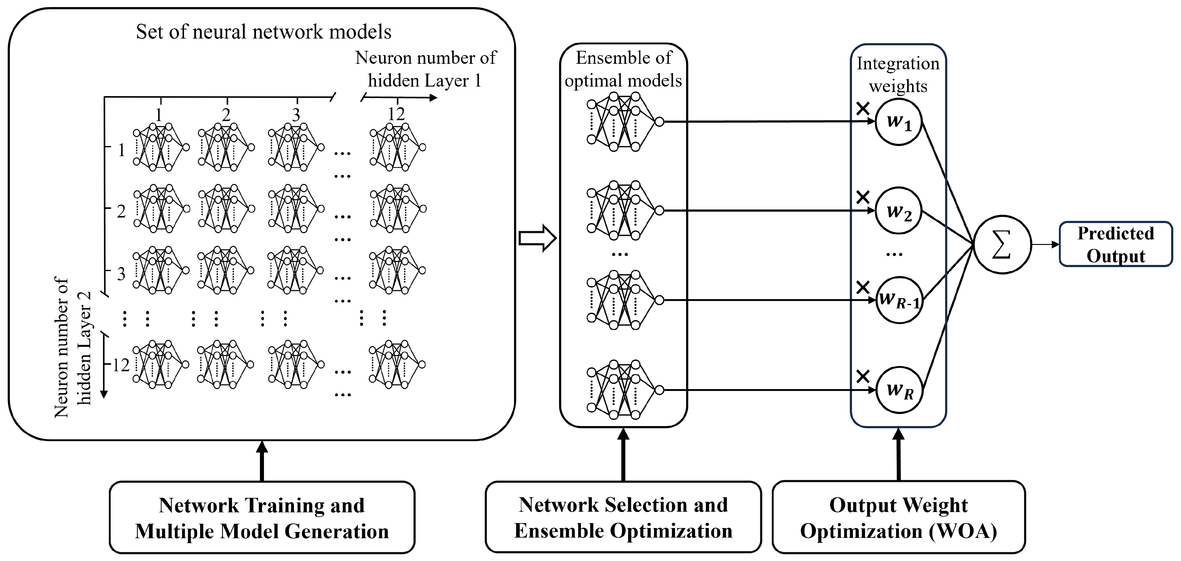
After performing cross-validation, the model is further refined by exploring different network architectures. The experiments compared the performance of models with one, two, and three hidden layers, revealing that while adding a second hidden layer improved performance, further layers led to diminishing returns and overfitting. Therefore, a two-hidden-layer architecture was selected for the final model. 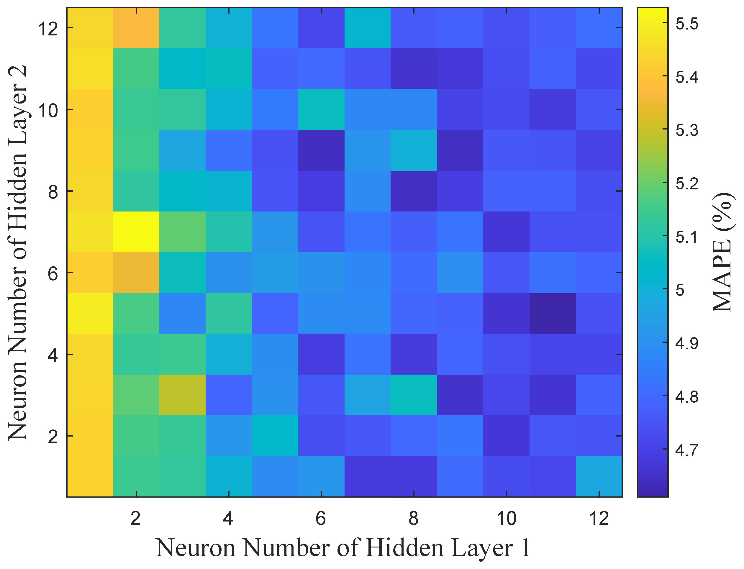Based on empirical guidelines [36], each hidden layer consists of a maximum of 12 neurons. This results in 144 distinct neural network configurations generated through various combinations of hyperparameters. These models are trained and evaluated on the model selection and ensemble optimization set to identify the best-performing architecture. The performance distribution of these 144 models is shown in Figure 9.

The number of neurons in the hidden layers plays a crucial role in determining the model’s complexity and learning capacity. More neurons allow the model to capture intricate features but increase the risk of overfitting, while fewer neurons may lead to insufficient feature learning, affecting prediction accuracy. This trade-off explains the variations in MAPE performance observed in Figure 9.

As shown in

Table 3. Performance comparison of neural network integration models with different hidden layer configurations.

Rank	Neurons in Layer 1	Neurons in Layer 2	MAPE (%)
1	11	5	4.61
2	6	9	4.64
3	8	8	4.64
4	9	9	4.64
5	9	3	4.65
6	8	11	4.66
7	10	5	4.66
8	11	3	4.66
9	10	2	4.67
10	10	7	4.67

, the performance of the neural network ensemble model under different hidden layer configurations is presented in detail. While the number of neurons does affect model performance, increasing the number of neurons does not always lead to improved performance. This suggests that model performance depends not only on the number of neurons but also on structural complexity and overfitting control. Too many neurons can introduce unnecessary complexity, reducing generalization ability and degrading performance. Therefore, balancing model complexity and generalization is crucial for optimizing neural network design.

Based on the above results, this study further explores the effect of using the average ensemble strategy (i.e., taking the average of the prediction results of multiple networks) under different neural networks to find the optimal number of neural networks. The basic idea of the average integration strategy is that by combining the prediction results of multiple neural networks, the uncertainty and volatility of the prediction of a single network can be reduced, thus improving the generalization ability and prediction accuracy of the whole model. As shown in Figure 10.

As the number of ensemble networks increases, model diversity initially improves, enhancing feature representation and reducing MAPE. However, an excessive number of networks increases computational complexity and the risk of overfitting, which may lead to performance degradation. The results demonstrate that the optimal balance between diversity and complexity is achieved with four networks, where the lowest MAPE is observed. Therefore, this study sets the number of integrated neural networks to four to ensure optimal performance and generalization ability.

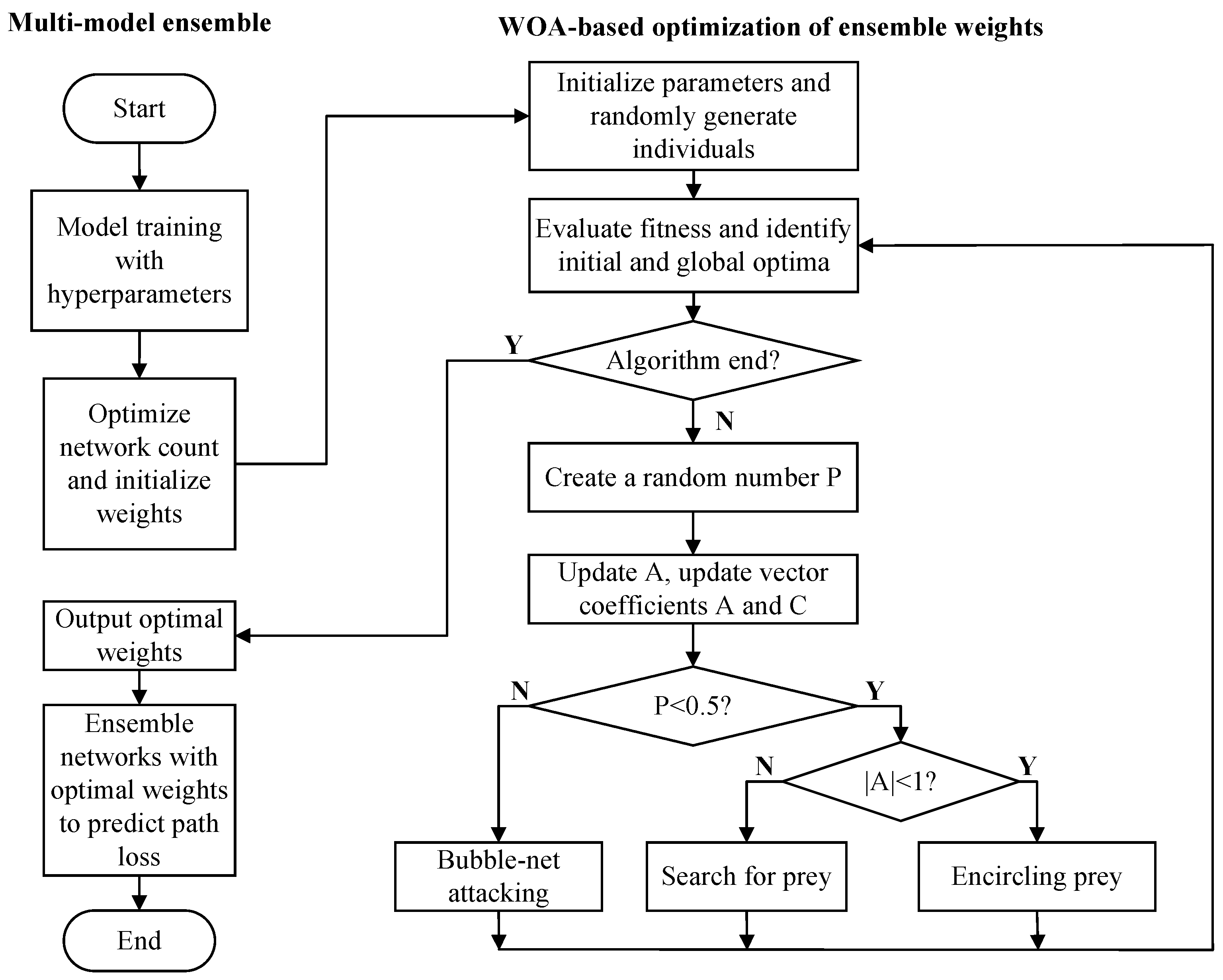
4.2. WOA-Based Output Weight Optimization

In path loss prediction, integrating multiple neural network models improves prediction accuracy, and further enhancement of overall performance can be achieved by optimizing the weight combinations of these models. The WOA used in this study configures the output weights of the models to effectively reduce prediction error. The optimized weights are applied to the integrated model and validated on the test set to further confirm its applicability in real-world scenarios. The algorithm parameters are shown in

Table 4. Parameters of the WOA algorithm.

Parameter	Value
Population size	50
Max Iterations	30
Initial value of A	2
Final value of A	0
Value of B	1
Range of C	[0, 2]

.

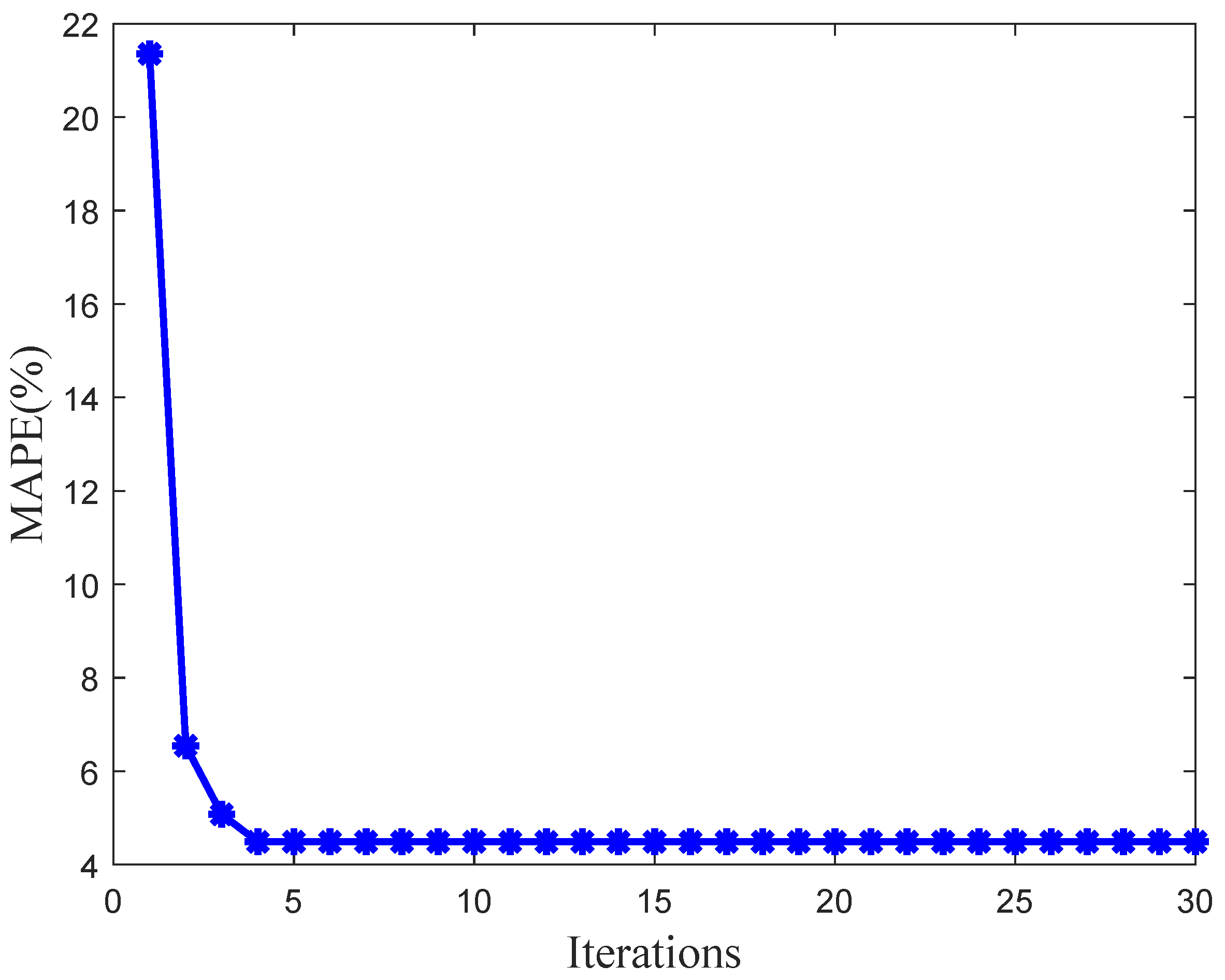
Figure 11 illustrates the variation of MAPE across generations during the WOA optimization process. The results show a rapid decline in MAPE during the initial generations, followed by stabilization after the fourth generation.

In the early iterations, WOA explores a broad solution space, quickly reducing MAPE as it searches for optimal weight combinations. As convergence progresses, the rate of improvement slows, and MAPE stabilizes, indicating that the algorithm has approached the optimal solution. This rapid convergence highlights WOA’s efficiency in weight optimization, demonstrating its capability to effectively minimize errors in the early stages and achieve stable performance in later iterations.

According to

Table 5. Configuration of neural network weights in the integrated model.

Weights	Value
$w_1$	0.3484
$w_2$	0.0035
$w_3$	0.4153
$w_4$	0.2326

, the weight configurations of the four finally selected neural networks in the integrated model are as follows: the 1st neural network weights 0.3484, indicating its significant role in the prediction results; the 2nd neural network weights 0.0035, contributing the least, reflecting its limited impact in the integrated model; the 3rd neural network weights 0.4153, contributing the most and significantly affecting the final prediction results; the 4th neural network has a weight of 0.2326, showing a moderate level of contribution. This weight configuration fully reflects the relative importance of each neural network in the integrated model. The integrated model optimizes the combination of predictions from multiple networks through differentiated weight allocation, thereby improving overall performance.

4.3. Computational Cost

Computational cost is a key consideration in model training and optimization. In this study, the computational cost of the model is mainly affected by the complexity of the neural network structure, the size of the dataset, and the optimization algorithm.

The experiments were carried out on computers equipped with the following hardware: the CPU is AMD Ryzen 5 7500F, manufactured by Advanced Micro Devices, Inc. (AMD), located in Sunnyvale, CA, USA with 8 cores and 16 threads; the GPU is NVIDIA GeForce RTX 4080, manufactured by NVIDIA Corporation, located in Santa Clara, CA, USA with 16 GB of video memory; the RAM is 32 GB; the storage is 1 TB NVMe SSD; and the operating system is Windows 11 Professional. The results show that the average BPNN training time is 1.55 s, and the overall time for filtering the integrated BPNN model combination is 17.31 s; the WOA optimization output weight time is 18.14 s.

4.4. Comparative Testing of Baseline Methods

In this experiment, to fully evaluate the performance of the proposed methods, we implemented six benchmark models: (1) CI, (2) CNN, (3) RNN, (4) GNN, (5) Transformer, (6) AutoML. Additionally, we included two ensemble models optimized using optimization algorithms to adjust the output weights of the models: (7) GA-Optimized Ensemble and (8) PSO-Optimized Ensemble. Suitable hyperparameter tuning techniques were applied to determine the optimal configuration for each model. Below is a detailed description of these models.

4.4.1. Path Loss Prediction Method Based on CI Modeling

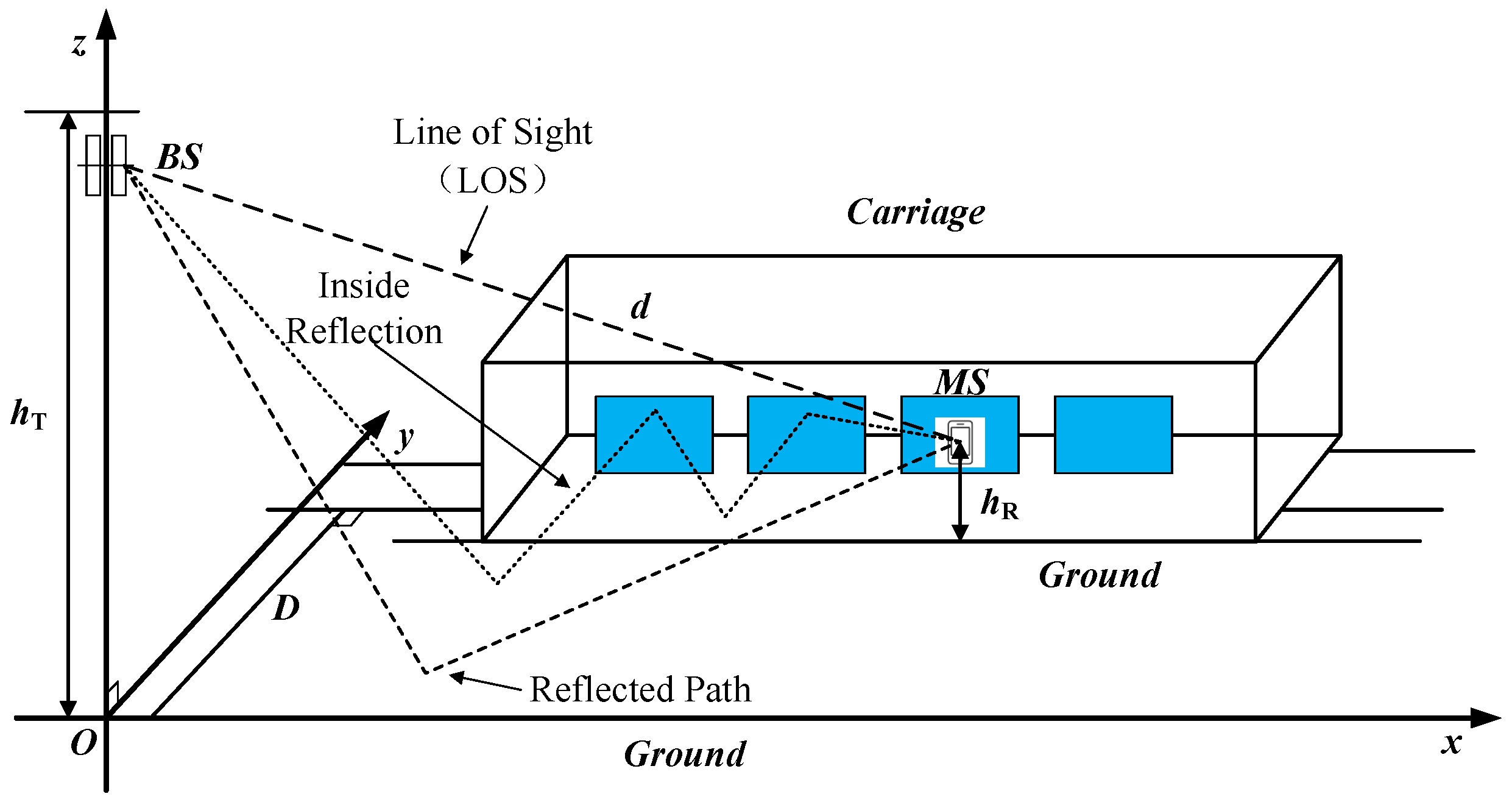
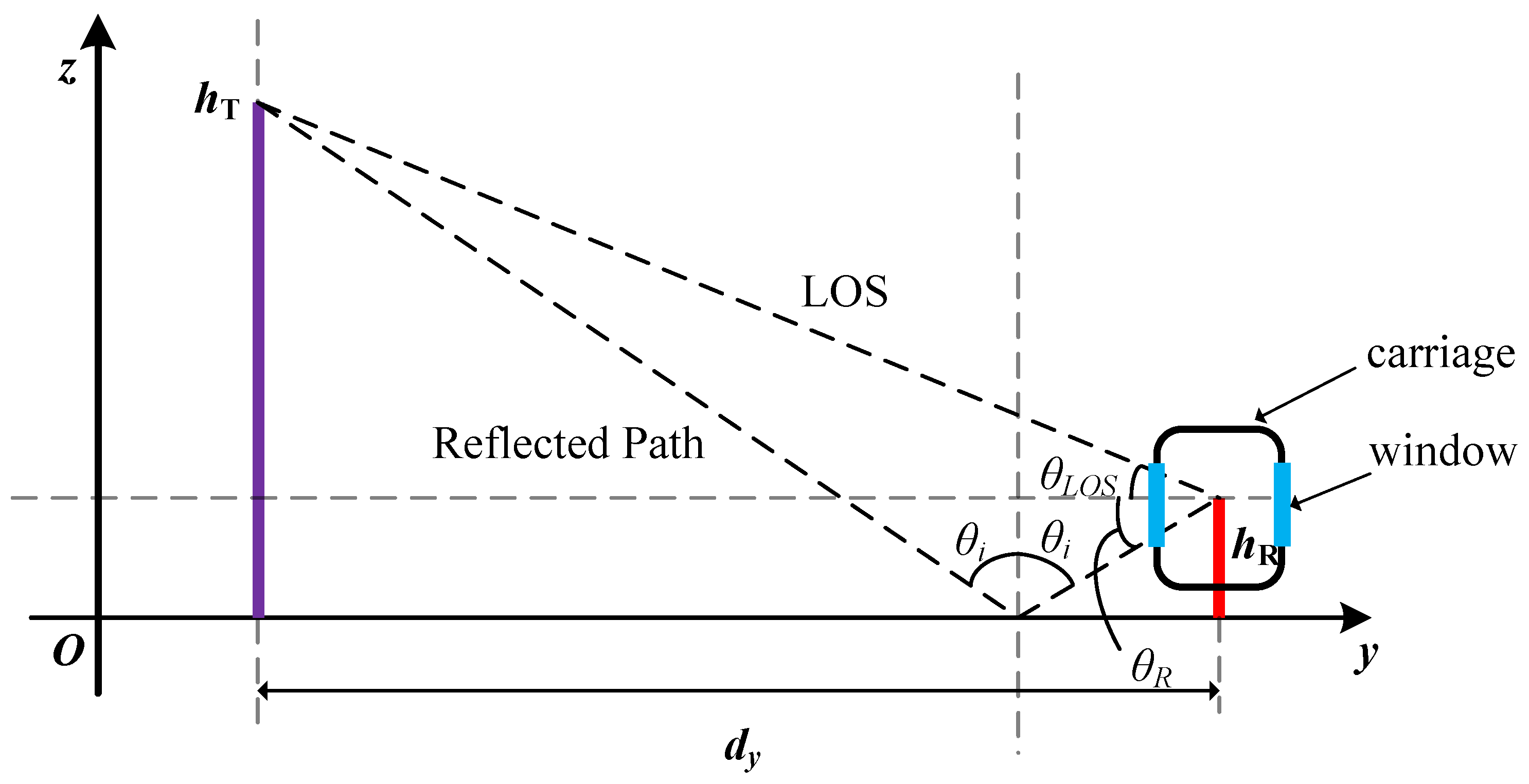
The CI model is an essential tool for designing and planning wireless communication systems. The primary purpose of the CI model is to predict the propagation loss of wireless signals in space based on the environmental characteristics and signal propagation conditions to evaluate the distribution of coverage and signal strength. This paper contains three different channels: the base station to the train, through the train window, and multiple reflections in the train. Its channel model is in the form of a cascade. To find the mathematical expression of the channel cascade, relying on the free-space neighboring reference distance model, this paper sets the model as follows:

$$P{L}_{CI}=10\mathrm{lo}{\mathrm{g}}_{10}{\left({\displaystyle \frac{4\pi d_0}{\lambda }}\right)}^2+10n\mathrm{lo}{\mathrm{g}}_{10}\left({\displaystyle \frac{d}{d_0}}\right)+X_{\sigma }$$

(14)

where $d_0$ represents the relative reference distance in free space, usually taken as 1 m. $\lambda$ represents the wavelength, and $X_{\sigma }$ represents a Gaussian random variable with a mean of 0 and a standard deviation of $\sigma$. n represents the composite factor comprising glass loss, vehicle reflections, etc. In this paper, a CI model is fitted to the seat path loss. After fitting, the value of n is 4.38.

4.4.2. Path Loss Prediction Method Based on CNN

Convolutional neural networks have shown great potential in handling various data-related tasks and have been used for path loss prediction in several studies [19,20,21]. We implemented a CNN model using PyTorch version 2.3.0 with hyperparameters, including the number of convolutional layers, the number of filters per layer, the convolutional kernel size, the pooling kernel size, and the activation function.

Table 6. Hyperparameter search space and selected values for CNN.

Hyperparameter	Search Space	Selected Value
Number of convolutional layers	{1, 2, 3}	2
Filters in the first conv layer	{16, 32, 64}	32
Filters in the second conv layer	{16, 32, 64}	64
Kernel size of the first conv layer	{3, 5}	3
Kernel size of the second conv layer	{1, 3}	1
Pooling kernel size	{2, 3}	2
Activation function	{“relu”, “tanh”, “sigmoid”}	“relu”

presents the optimal combination of hyperparameters for the convolutional neural network determined through the hyperparameter optimization process.

4.4.3. Path Loss Prediction Method Based on RNN

Recurrent neural networks are well suited for processing sequential data and have applications in some scenarios related to path loss prediction [17,22]. We implemented a recurrent neural network model using PyTorch version 2.3.0 with hyperparameters that include the input feature dimensions, the number of hidden layer units, the type of activation function, and the setting of the fully connected layers.

Table 7. Hyperparameter search space and selected values for RNN.

Hyperparameter	Search Space	Selected Value
Input feature dimension	{1, 2, 3}	1
Number of hidden layer units	{32, 64, 128}	64
RNN activation function	{“tanh”, “relu”}	“tanh”
Fully connected layer output dimension	{1, 2}	1

shows the optimal combination of hyperparameters for the recurrent neural network determined through the hyperparameter optimization process.

4.4.4. Path Loss Prediction Method Based on GNN

Graph neural networks have recently been explored for path loss prediction in [23]. We implemented this network based on PyTorch version 2.3.0 using appropriate graph neural network-related libraries. The hyperparameters of this network are the number of graph convolution layers, the number of hidden units per layer, the activation function, the K-value of the K-nearest neighbor, the learning rate, the weight decay coefficient, and the type of loss function.

Table 8. Hyperparameter search space and selected values for GNN.

Hyperparameter	Search Space	Selected Value
Number of GCN layers	{2, 3, 4}	3
Units in first hidden layer	{32, 64, 128}	64
Units in second hidden layer	{32, 64, 128}	64
Activation function	{“relu”, “tanh”, “sigmoid”}	“relu”
K value for KNN	{3, 5, 7}	5
Learning rate	{0.0001, 0.001, 0.01}	0.001
Weight decay	{$1\times {10}^{-4}$, $5\times {10}^{-4}$, $1\times {10}^{-3}$}	$5\times {10}^{-4}$
Loss function	{“MSE”, “SmoothL1Loss”}	“SmoothL1Loss”

presents the optimal combination of hyperparameters for the graph neural network determined through the hyperparameter optimization process.

4.4.5. Path Loss Prediction Method Based on Transformer

Transformer has emerged as a novel and powerful architecture in recent years, and its application in path loss prediction shows great potential. We implemented this model using the PyTorch version 2.3.0 framework, leveraging relevant libraries for Transformer architectures. The hyperparameters of this network include the number of Transformer encoder layers, the model embedding dimension, the number of attention heads, the activation function, the learning rate, the weight decay coefficient, and the type of loss function.

Table 9. Hyperparameter search space and selected values for Transformer.

Hyperparameter	Search Space	Selected Value
Encoder Layers	{1, 2, 3}	2
Embedding Dimension	{16, 32, 64, 128}	64
Attention Heads	{2, 4, 8}	4
Activation Function	{“relu”, “gelu”}	“relu”
Learning Rate	{0.00005, 0.0001, 0.001}	0.001
Weight Decay	{$1\times {10}^{-4}$, $5\times {10}^{-4}$, $5\times {10}^{-3}$}	$5\times {10}^{-4}$
Loss Function	{“MSE”, “SmoothL1Loss”}	“SmoothL1Loss”

shows the optimal combination of hyperparameters for the Transformer network determined through the hyperparameter optimization process.

4.4.6. Path Loss Prediction Method Based on AutoML Tool

Automated Machine Learning has emerged as a revolutionary approach in the field of machine learning. It automates the often complex processes of model selection and hyperparameter tuning. In this study, we harnessed the power of the TPOTRegressor from the spot library to tackle the path loss prediction problem.

The parameters of the TPOTRegressor are crucial in determining the effectiveness and efficiency of the automated model search.

Table 10. Parameter and their values for AutoML tool.

Parameter	Value
Generations	5
Population Size	30
Random State	42
Crossover Rate	0.8
Mutation Rate	0.2

presents the key hyperparameters and their selected values for our path loss prediction task:

After setting the parameters, the AutoML tool automatically searched for the optimal machine-learning pipeline and found an ensemble model for path loss prediction. This ensemble model combines Stochastic Gradient Descent (SGD) and Random Forest regression.

Table 11. Key parameter settings of the regression methods used in AutoML tool.

Regression Method	Parameter	Setting
Stochastic Gradient Descent	Regularization Type	L1 + L2
	L1 Regularization Ratio	75%
	L2 Regularization Ratio	25%
	Regularization Penalty	None
	Initial Learning Rate	0.1
	Learning Rate Strategy	Gradual decay
	Learning Rate Decay	Controlled factor
	Intercept Calculation	Enabled
	Loss Function Sensitivity	Low error sensitivity
Random Forest	Number of Trees	100
	Feature Ratio	5% features
	Minimum Samples per Leaf	7
	Minimum Samples for Split	17

presents the key parameter settings of the two regression methods:

4.4.7. Path Loss Prediction Method Based on GA—Optimized Ensemble Model

Genetic Algorithm is employed to optimize the output weights of the multi-neural network ensemble model for predicting path loss in high-speed train carriages. This method aims to improve the prediction accuracy by identifying the optimal combination of weights for the ensemble model.

Table 12. Parameters for GA optimization.

Parameter	Optimal Value
Population Size	50
Crossover Probability	0.8
Mutation Probability	0.01
Number of Generations	30

shows the optimal combination of parameters for the GA-optimized output weights.

4.4.8. Path Loss Prediction Method Based on PSO—Optimized Ensemble Model

Particle Swarm Optimization is applied to optimize the output weights of the multi-neural network ensemble model for path loss prediction. PSO is a meta-heuristic optimization algorithm that finds the best combination of output weights in a multi-dimensional space.

Table 13. Parameters for PSO optimization.

Parameter	Optimal Value
Number of Particles	50
Inertia Weight	0.7
Cognitive Coefficient	1.4
Social Coefficient	1.4
Maximum Number of Iterations	30

shows the optimal combination of parameters for the PSO-optimized output weights.

4.5. Predicted Results

Table 14. Error statistics of different methods in the testing phase.

Method	RMSE (dB)	MAE (dB)	MAPE (%)	R2
CI	8.39	6.82	6.04	0.24
CNN	7.39	5.53	4.74	0.41
RNN	7.85	6.31	5.55	0.34
GNN	8.30	6.61	5.78	0.26
Transformer	7.34	5.97	5.25	0.42
AutoML	7.01	5.53	4.82	0.47
Ensemble Model with GA-Optimized	7.25	5.78	5.02	0.43
Ensemble Model with PSO-Optimized	7.10	5.61	4.85	0.45
Ensemble Model with WOA-Optimized	6.92	5.37	4.67	0.48

shows the performance of different path loss prediction methods on the test set. According to the data, the neural network integration model optimized by WOA output weights, proposed in this paper, performs exceptionally well in predicting the path loss of HSR seats. Compared to CI, CNN, RNN, GNN, Transformer, AutoML, and the ensemble models with GA-Optimized and PSO-Optimized output weights, the proposed model significantly outperforms the others in four key metrics: RMSE, MAE, MAPE, and R².

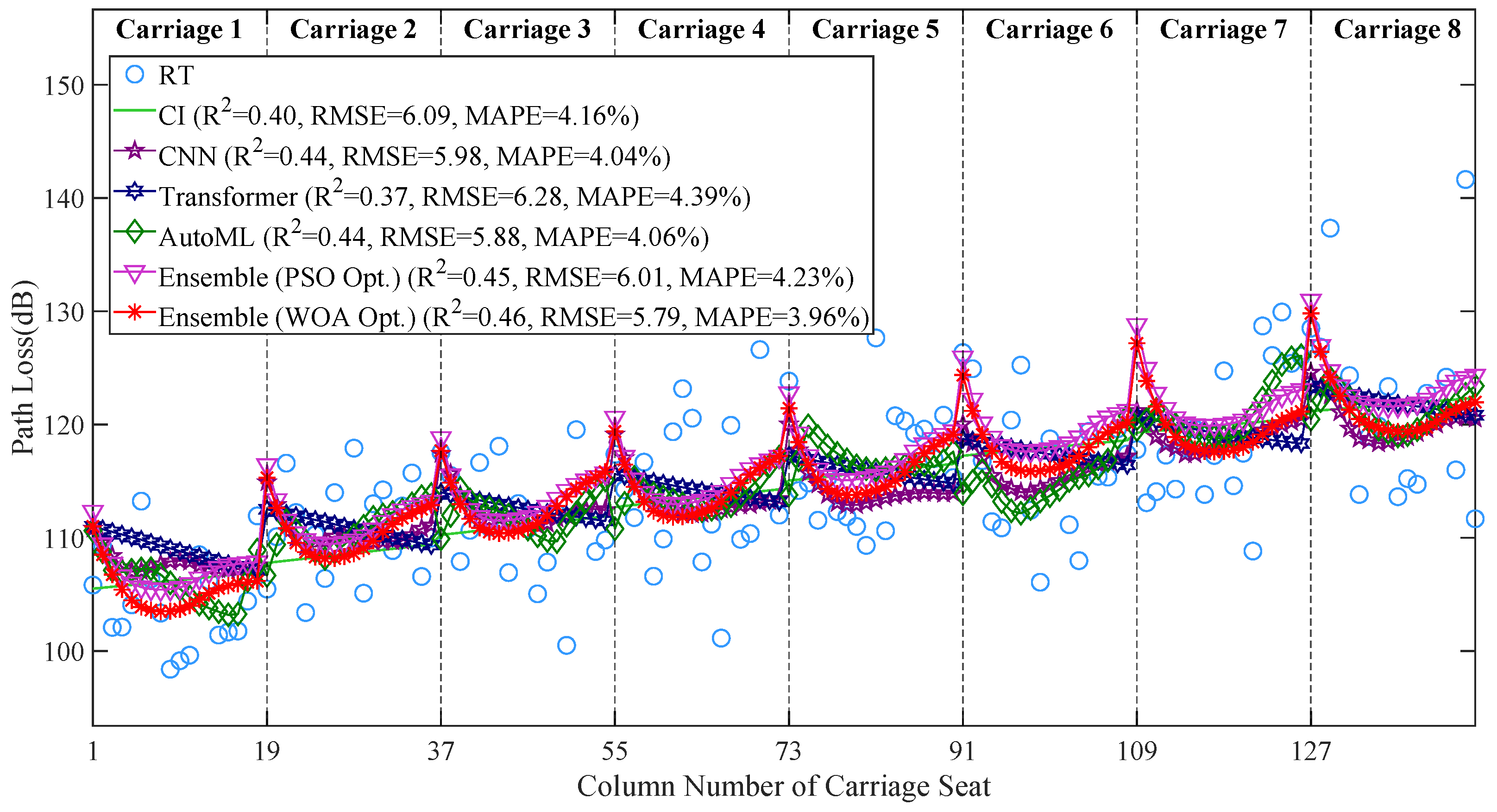
To further assess the robustness of the proposed model, we select representative data points from location E, with the receiving antenna positioned at height III. The prediction results are compared and analyzed against those of the CI model, CNN, Transformer, AutoML, and the ensemble model optimized using the PSO. As illustrated in Figure 12, the legend provides detailed annotations, where Ensemble (PSO Opt.) represents the ensemble model optimized using the PSO, and Ensemble (WOA Opt.) denotes the ensemble model optimized using the WOA. Additionally, the performance metrics for each method, calculated based on their predictions relative to the RT values, are displayed in the legend for clarity.

As shown in the figure, the WOA-optimized ensemble model stands out, with key performance metrics of R² = 0.46, RMSE = 5.79 dB, and MAPE = 3.96%, all of which outperform the other models. Furthermore, the model exhibits minimal fluctuation in prediction curves across different carriages, demonstrating excellent robustness. Unlike other models, which show significant deviation from the actual values or poor stability, this model maintains consistent performance despite changes in carriage position, highlighting its superior ability to withstand environmental interference and maintain stability across different spatial locations.

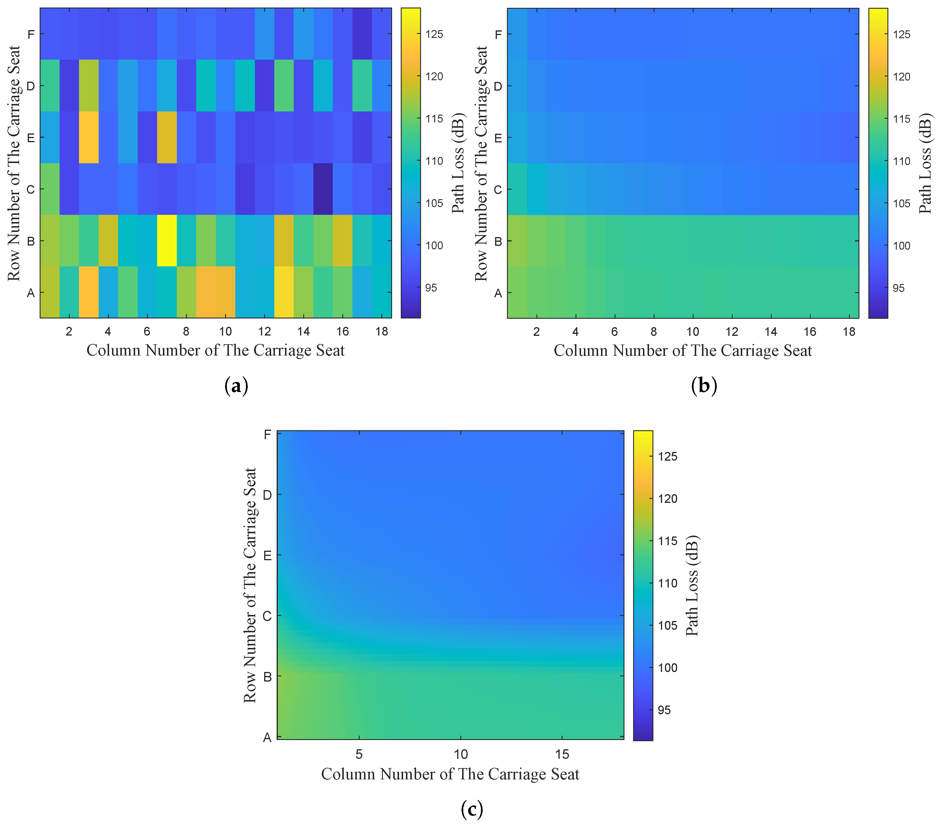
To deeply analyze the predictive effect of the models in a single carriage, the data at the height III position in the first carriage is selected to show the comparison between the original data and the predicted value of the path loss. Figure 13a shows the distribution of the path loss data in the block obtained by applying WI simulation. Figure 13b shows the distribution of path loss predictions generated by the integrated neural network prediction method proposed in this paper. Based on the prediction results in Figure 13b, Figure 13c uses a linear interpolation method to interpolate the signal path loss across the entire compartment plane, which is used to predict the path loss distribution over a broader range within the compartment.

In Figure 13, the horizontal axis represents the number of seat rows in the compartment, the vertical axis represents the position, and the color shade directly reflects the magnitude of the predicted or actual path loss. The predicted values of the path loss of the model in this paper are consistent with the original data in terms of distribution, indicating that the model has a high accuracy in predicting the path loss at the height III position of a single compartment. The feasibility of the model in predicting the field strength distribution in the compartment is demonstrated.

5. Conclusions

In this study, our proposed field strength prediction model for high-speed rail carriages based on multi-neural network integration combined with the whale optimization algorithm shows good prediction performance in the current train scenario. However, the model still has several aspects that can be further optimized.

5.1. Concluding Remarks

In model construction and optimization, we successfully built a multi-neural network integration model and optimized its output weights using the Whale Optimization Algorithm. Through hyperparameter tuning, we determined the optimal model structure and adopted techniques such as the tanh activation function, Adam optimizer, early stopping, and L2 regularization to prevent overfitting and ensure efficient convergence. The model demonstrates excellent performance in predicting field strength in high-speed rail carriages. Future work can explore more efficient hyperparameter selection strategies based on the existing model framework.

For data processing and dataset construction, we integrated dual-path modeling, on-site channel measurements, and ray-tracing (RT) simulations to create a high-precision training dataset. Channel measurements in a CR400BF train compartment provided real data, while RT simulations generated a dataset of 4320 samples, forming a solid foundation for model training. Future work can incorporate data from diverse environments to enhance model adaptability.

In model evaluation and comparison, we employed multiple metrics (RMSE, MAE, MAPE, and R²) to assess model performance. Results show our model outperforms traditional and comparative models, confirming its effectiveness. Additionally, our model demonstrates strong robustness under the specified seat conditions, further validating its stability and adaptability in practical applications. The evaluation approach in this study provides a valuable reference for future model refinements.

5.2. Future Work

Future work will expand data acquisition to better adapt the model to evolving railway scenarios. With the introduction of CR450 high-speed trains, we will document carriage structures, electromagnetic properties, and layout details. High-precision field strength measurements will be taken at key locations inside the train, covering terrains like tunnels and viaducts. Data will also be collected under varying operating conditions, including different speeds, operational hours, and base station distributions, to analyze their effects on signal propagation. This enhanced dataset will improve model training and ray-tracing accuracy and introduce interference factors to strengthen robustness. Additionally, train speed information will be integrated to refine the multipath model for better interference handling.

Leveraging this new data, we will further optimize the multi-neural network integration model through cross-validation and grid search, refining network architecture, hyperparameters, and regularization techniques. We will explore the model structure for innovations such as attention mechanisms to enhance feature extraction. Additionally, we will integrate recurrent neural networks (RNNs) and their variants (LSTM, GRU) to improve the handling of dynamic signal propagation.

Future research will focus on refining hyperparameter selection through automated optimization methods. This approach will ensure efficient and accurate identification of key parameters while avoiding local optima. The use of this approach will streamline model tuning and further enhance predictive performance.

Transfer learning will help the model quickly adjust to new train types and materials, improving adaptability across different propagation conditions. By leveraging pre-trained knowledge, we aim to reduce data requirements and training time for new scenarios. Continuous monitoring of advancements in train technologies and materials will further support ongoing model optimization and expansion into diverse application contexts.

References

1. Agiwal, M.; Roy, A.; Saxena, N. Next generation 5G wireless networks: A comprehensive survey. IEEE Commun. Surv. Tutor. 2016, 18, 1617–1655. [Google Scholar] [CrossRef]
2. He, R.; Ai, B.; Zhong, Z.; Yang, M.; Chen, R.; Ding, J.; Ma, Z.; Sun, G.; Liu, C. 5G for railways: Next generation railway dedicated communications. IEEE Commun. Mag. 2022, 60, 130–136. [Google Scholar] [CrossRef]
3. Noh, G.; Hui, B.; Kim, I. High speed train communications in 5G: Design elements to mitigate the impact of very high mobility. IEEE Wirel. Commun. 2020, 27, 98–106. [Google Scholar] [CrossRef]
4. Guo, H.; Wei, M.; Yu, J.; Li, X. Research on 5G High Speed Train Coverage Enhancement Technology. In Proceedings of the 2024 IEEE International Symposium on Broadband Multimedia Systems and Broadcasting (BMSB), Toronto, ON, Canada, 19–21 June 2024; pp. 1–5. [Google Scholar]
5. Gonzalez-Plaza, A.; Moreno, J.; Val, I.; Arriola, A.; Rodriguez, P.M.; Jimenez, F.; Briso, C. 5G communications in high speed and metropolitan railways. In Proceedings of the 2017 11th European Conference on Antennas and Propagation (EUCAP), Paris, France, 19–24 March 2017; pp. 658–660. [Google Scholar]
6. He, D.; Ai, B.; Guan, K.; Zhong, Z.; Hui, B.; Kim, J.; Chung, H.; Kim, I. Channel measurement, simulation, and analysis for high-speed railway communications in 5G millimeter-wave band. IEEE Trans. Intell. Transp. Syst. 2017, 19, 3144–3158. [Google Scholar] [CrossRef]
7. Fugen, T.; Maurer, J.; Kayser, T.; Wiesbeck, W. Capability of 3-D ray tracing for defining parameter sets for the specification of future mobile communications systems. IEEE Trans. Antennas Propag. 2006, 54, 3125–3137. [Google Scholar] [CrossRef]
8. Zhao, H.; Chen, Y.; Wang, X.; Saleem, A.; Zheng, G. Discovery and Analysis of Brewster’s Angle Effect for Path Loss in High-Speed Railway Scenarios. IEEE Wirel. Commun. Lett. 2024, in press. [Google Scholar] [CrossRef]
9. Yuan, Y.; He, R.; Ai, B.; Niu, Y.; Yang, M.; Wang, G.; Chen, R.; Li, Y.; Li, J.; Ding, J. A 3D geometry-based reconfigurable intelligent surfaces-assisted MmWave channel model for high-speed train communications. IEEE Trans. Veh. Technol. 2023, 73, 1524–1539. [Google Scholar] [CrossRef]
10. Chen, B.; Zhong, Z.; Ai, B.; Michelson, D.G. A geometry-based stochastic channel model for high-speed railway cutting scenarios. IEEE Antennas Wirel. Propag. Lett. 2014, 14, 851–854. [Google Scholar] [CrossRef]
11. Yang, J.; Ai, B.; Guan, K.; He, D.; Lin, X.; Hui, B.; Kim, J.; Hrovat, A. A geometry-based stochastic channel model for the millimeter-wave band in a 3GPP high-speed train scenario. IEEE Trans. Veh. Technol. 2018, 67, 3853–3865. [Google Scholar] [CrossRef]
12. Zhou, L.; Luan, F.; Zhou, S.; Molisch, A.F.; Tufvesson, F. Geometry-based stochastic channel model for high-speed railway communications. IEEE Trans. Veh. Technol. 2019, 68, 4353–4366. [Google Scholar] [CrossRef]
13. Feng, Y.; Wang, R.; Zheng, G.; Saleem, A.; Xiang, W. A 3D Non-Stationary Small-Scale Fading Model for 5G High-Speed Train Massive MIMO Channels. IEEE Trans. Intell. Transp. Syst. 2024, 25, 16490–16505. [Google Scholar] [CrossRef]
14. Zhou, T.; Li, H.; Wang, Y.; Liu, L.; Tao, C. Channel modeling for future high-speed railway communication systems: A survey. IEEE Access 2019, 7, 52818–52826. [Google Scholar] [CrossRef]
15. Wen, J.; Zhang, Y.; Yang, G.; He, Z.; Zhang, W. Path loss prediction based on machine learning methods for aircraft cabin environments. IEEE Access 2019, 7, 159251–159261. [Google Scholar] [CrossRef]
16. Huang, J.; Wang, C.-X.; Bai, L.; Sun, J.; Yang, Y.; Li, J.; Tirkkonen, O.; Zhou, M.-T. A big data enabled channel model for 5G wireless communication systems. IEEE Trans. Big Data 2018, 6, 211–222. [Google Scholar] [CrossRef]
17. Jiang, W.; Schotten, H.D. Multi-antenna fading channel prediction empowered by artificial intelligence. In Proceedings of the 2018 IEEE 88th Vehicular Technology Conference (VTC-Fall), Chicago, IL, USA, 27–30 August 2018; pp. 1–6. [Google Scholar]
18. Zhu, Y.; Dong, X.; Lu, T. An adaptive and parameter-free recurrent neural structure for wireless channel prediction. IEEE Trans. Commun. 2019, 67, 8086–8096. [Google Scholar] [CrossRef]
19. Meenalakshmi, M.; Chaturvedi, S.; Dwivedi, V.K. Enhancing channel estimation accuracy in polar-coded MIMO–OFDM systems via CNN with 5G channel models. AEU-Int. J. Electron. Commun. 2024, 173, 155016. [Google Scholar] [CrossRef]
20. Xiong, L.; Zhang, Z.; Yao, D. A novel real-time channel prediction algorithm in high-speed scenario using convolutional neural network. Wirel. Netw. 2022, 28, 621–634. [Google Scholar] [CrossRef]
21. Stenhammar, O.; Fodor, G.; Fischione, C. A comparison of neural networks for wireless channel prediction. IEEE Wirel. Commun. 2024, 31, 235–241. [Google Scholar] [CrossRef]
22. Shahabodini, S.; Mansoori, M.; Abouei, J.; Plataniotis, K.N. Recurrent neural network and federated learning based channel estimation approach in mmWave massive MIMO systems. Trans. Emerg. Telecommun. Technol. 2024, 35, e4926. [Google Scholar] [CrossRef]
23. Wang, X.; Guan, K.; He, D.; Hrovat, A.; Liu, R.; Zhong, Z.; Al-Dulaimi, A.; Yu, K. Graph Neural Network enabled Propagation Graph Method for Channel Modeling. IEEE Trans. Veh. Technol. 2024, 73, 12280–12289. [Google Scholar] [CrossRef]
24. Dietterich, T.G. Ensemble methods in machine learning. In Proceedings of the International Workshop on Multiple Classifier Systems, Cagliari, Italy, 21–23 June 2000; pp. 1–15. [Google Scholar]
25. Schwenker, F. Ensemble methods: Foundations and algorithms [book review]. IEEE Comput. Intell. Mag. 2013, 8, 77–79. [Google Scholar] [CrossRef]
26. Breiman, L. Bagging predictors. Mach. Learn. 1996, 24, 123–140. [Google Scholar] [CrossRef]
27. Altman, N.; Krzywinski, M. Ensemble methods: Bagging and random forests. Nat. Methods 2017, 14, 933–935. [Google Scholar] [CrossRef]
28. Freund, Y.; Schapire, R.E. A decision-theoretic generalization of online learning and an application to boosting. J. Comput. Syst. Sci. 1997, 55, 119–139. [Google Scholar] [CrossRef]
29. Chen, T.; Guestrin, C. XGBoost: A scalable tree boosting system. In Proceedings of the 22nd ACM SIGKDD International Conference on Knowledge Discovery and Data Mining, San Francisco, CA, USA, 13–17 August 2016; pp. 785–794. [Google Scholar]
30. Wolpert, D.H. Stacked generalization. Neural Netw. 1992, 5, 241–259. [Google Scholar] [CrossRef]
31. Sharma, S.R.; Singh, B.; Kaur, M. A novel approach of ensemble methods using the stacked generalization for high-dimensional datasets. IETE J. Res. 2023, 69, 6802–6817. [Google Scholar] [CrossRef]
32. Ludmila, I. Combining Pattern Classifiers: Methods and Algorithms; Wiley: Hoboken, NJ, USA, 2004. [Google Scholar]
33. Leon, F.; Floria, S.-A.; Bădică, C. Evaluating the effect of voting methods on ensemble-based classification. In Proceedings of the 2017 IEEE International Conference on Innovations in Intelligent Systems and Applications (INISTA), Gdynia, Poland, 3–5 July 2017; pp. 1–6. [Google Scholar]
34. Moraitis, N.; Tsipi, L.; Vouyioukas, D.; Gkioni, A.; Louvros, S. Performance evaluation of machine learning methods for path loss prediction in rural environment at 3.7 GHz. Wirel. Netw. 2021, 27, 4169–4188. [Google Scholar] [CrossRef]
35. Moraitis, N.; Tsipi, L.; Vouyioukas, D.; Gkioni, A.; Louvros, S. On the assessment of ensemble models for propagation loss forecasts in rural environments. IEEE Wirel. Commun. Lett. 2022, 11, 1097–1101. [Google Scholar] [CrossRef]
36. Li, H.; Mao, K.; Ye, X.; Zhang, T.; Zhu, Q.; Wang, M.; Ge, Y.; Li, H.; Ali, F. Air-to-Ground Path Loss Model at 3.6 GHz under Agricultural Scenarios Based on Measurements and Artificial Neural Networks. Drones 2023, 7, 701. [Google Scholar] [CrossRef]
37. Kwon, B.; Son, H. Accurate Path Loss Prediction Using a Neural Network Ensemble Method. Sensors 2024, 24, 304. [Google Scholar] [CrossRef]
38. Mirjalili, S.; Lewis, A. The whale optimization algorithm. Adv. Eng. Softw. 2016, 95, 51–67. [Google Scholar] [CrossRef]
Figure 1. The communication scenario between the base station and the terminal in HSR.
Applsci 15 02709 g001
Figure 2. Schematic diagram of the base station-train two-path communication scenario.
Applsci 15 02709 g002
Figure 3. Channel measurement campaigns in the HSR scenario.
Applsci 15 02709 g003
Figure 4. RT simulation scenario.
Applsci 15 02709 g004
Figure 5. Comparison of Received Power: Theoretical (Based on Two-path Model in Section 2.2, see Equation (1)), Measurement (Section 2.3), and Simulation (Ray tracing with parameters adjusted in Section 2.4).
Applsci 15 02709 g005
Figure 6. Seat layout inside the carriage: (a) Cross-section view of the seat arrangement; (b) Top view of the carriage seating layout.
Applsci 15 02709 g006
Figure 7. Field strength prediction method for HSR carriages.
Applsci 15 02709 g007
Figure 8. Flowchart of the WOA-optimized ensemble model method.
Applsci 15 02709 g008
Figure 9. MAPE performance of 144 models with varying hidden layer neuron counts.
Applsci 15 02709 g009
Figure 10. MAPE curve versus number of ensemble networks.
Applsci 15 02709 g010
Figure 11. WOA iterative optimization curve.
Applsci 15 02709 g011
Figure 12. Comparison of prediction results for Height III and Position E.
Applsci 15 02709 g012
Figure 13. Path loss distribution at height III in the first carriage: (a) WI simulation, (b) The method in this paper, and (c) Interpolation distribution based on the method in this paper.
Applsci 15 02709 g013