Fréchet-Derivative-Based Global Sensitivity Analysis and Its Physical Meanings in Structural Design

Abstract

Sensitivity analysis is essential for uncertainty-based structural design and analysis, especially global sensitivity analysis, which can reflect the overall physical properties of large and complex computational models with stochastic parameters. In recent decades, a variety of global sensitivity indices (GSIs) have been extensively developed based on the distinct perspectives of global sensitivity analysis, in which the most common GSIs are variance-based, moment-independent, and failure-probability-based. In this work, a newly developed Fréchet-derivative-based GSI (Fre-GSI) is discussed. Properties of the Fre-GSI related to the measure and direction are first investigated. Then, a functional perspective of global sensitivity analysis is proposed, with the physical meanings of the four GSIs illustrated. Practical links of the Fre-GSI with the other three classical GSIs are derived analytically. Numerical examples are studied to verify the proposed links, and the specific advantages of the four GSIs are discussed.

1. Introduction

Sensitivity analysis, known as a powerful means for detecting which model inputs may have influential impacts on the model output(s), has played an important role in computational model-based structural design, evaluation, and optimization in various fields, e.g., structural engineering [1,2,3], wind engineering [4,5], bridge engineering [6], and aerospace engineering [7,8]. When the basic input variables are deterministic, the partial derivatives of the model output (quantity of interest, QoI), with respect to the input variables, are widely employed as sensitivity indices belonging to the local category [9]. However, if the QoI concern is stochastic due to the aleatory uncertainty of input parameters, the global sensitivity index (GSI), which can provide more quantitative information, should be seriously taken into account [10,11]. On the definition of “global sensitivity analysis” given by Saltelli et al. [12], wherein the whole variation domain of the inputs is considered, many GSIs have been established in the literature. Among them, perhaps the most notable and classical GSIs are variance-based GSI [13,14], moment-independent GSI [15,16], and failure-probability-based GSI [17,18]. Note that the studied failure-probability-based GSI is also called the “reliability-oriented sensitivity index” [8,19], or the “reliability sensitivity index” [20]. To avoid ambiguity, the term “failure-probability-based GSI” is adopted throughout this study.

The variance-based GSI (a.k.a. Sobol’ index) quantifies the impact of one input or the interaction effect of two or more inputs on the variance of the QoI. The moment-independent GSI (e.g., Borgonovo’s $\delta$-index) is based on the absolute difference between the conditional distribution and the unconditional one. For most engineering issues that adopt nonlinear and non-monotonic models, the “size” effect of sensitivity can be reflected by these two GSIs with non-negative values, while the “direction” effect of sensitivity can only be observed via data visualization [21,22], e.g., in the form of 2D/3D scatter plots, box plots, cobweb plots, etc. In fact, the direction effect can be more essential for structural analysis, especially for reliability-based design optimization [11]. In this circumstance, the direction property of sensitivity is supposed to be integrated into the optimization process rather than having data visualized in each iteration. Hence, the failure probability-based GSI, which can reflect both the size and direction properties of the sensitivity, has attracted a lot of attention in reliability engineering. Nonetheless, the information, which failure probability can provide to quantify the uncertainty, is somewhat limited. In other words, the uncertainty of the QoI may not be completely characterized if only the probability of failure is taken into account. Similarly, Borgonovo [23] showed that non-informative results may be obtained when one relies on variance as the sole representative.

In spite of widespread applications of the different GSIs mentioned above, there still lacks an informative GSI, which is supposed to perform the following: (1) quantitatively detect the most dominant model inputs (importance measure); (2) comprehensively describe the most influential directions (direction indicator); (3) intelligently reveal physical mechanisms (as a probe) of complex models with uncertain parameters. Most of the available GSIs satisfy the first feature, but only some of them hold the second feature, and they rarely posses the third one.

For the above-mentioned requirements, the perturbed-law-based sensitivity index [24] (called DMBRSI in its first appearance [20]) can be an appropriate solution. It can measure how wide the change is in the probability of failure when shifting the mean values or the variances of input variables. One may immediately think of the following: What sensitivity information can we obtain if we measure how the output probability density function (PDF, rather than the failure probability) varies when the input PDF (not only with respect to the mean or variance) is changed? This thought appeared in [10], wherein a new GSI based on the concept of the Fréchet derivative (short for Fre-GSI) was proposed. Nevertheless, there are still some issues with Fre-GSI, which need to be discussed. More importantly, how different GSIs serve the global sensitivity analysis and what intrinsic connections are between Fre-GSI and other GSIs have not been explored as yet.

Although many GSIs are worth discussing, this study mainly focuses on variance-based GSI, moment-independent GSI, failure-probability-based GSI, and Fre-GSI. Firstly, the importance measure and direction indicator of Fre-GSI are given in this work. Some valuable properties of these two quantities are studied. Then, a unified description from a functional perspective is proposed to explain the differences as well as the similarities between the four GSIs. Some practical links between the Fre-GSI and the three classical GSIs are derived accordingly. Test examples are studied to verify the proposed links, and the specific advantages of the four GSIs, which serve for global sensitivity analysis, are also illustrated.

The novelty of this paper lies in three aspects: (1) a unified description is proposed for understanding the similarities and differences between the four GSIs from a functional perspective; (2) practical links are derived between the Fre-GSI and the variance-based GSI, moment-independent GSI, and failure-probability-based GSI; (3) a complementary nature of the four GSIs is revealed throughout numerical and engineering applications.

2. Primary Concepts and Assumptions in This Work

Throughout this work, we consider a stochastic parametric model, or more specifically, a computational model with uncertain parameters, which is represented by

$$X=g\left(\mathbf{\Theta }\right),$$

(1)

where the linear or nonlinear mapping $g(·):{\mathbb{R}}^s\mapsto {\mathbb{R}}^1$ is assumed to be square-integrable, $\mathbf{\Theta }={({\mathrm{\Theta }}_1,{\mathrm{\Theta }}_2,\cdots ,{\mathrm{\Theta }}_s)}^{\top }\in {\mathbb{R}}^s$ is an s-dimensional random vector, and $X\in {\mathbb{R}}^1$ is the quantity of interest (QoI) of output.

It must be emphasized that the QoI may be multivariable or even time-dependent for many engineering practices. At present, global sensitivity analysis for this type of issue is still filled with challenges, see [1,25,26]. For simplicity, only the univariate and time-invariant QoIs are of concern in this work.

Consider a more rigorous mathematical definition of Equation (1). Define the triple $(\mathrm{\Omega },\mathcal{F},\mathbb{P})$ as the probability space, where $\mathrm{\Omega }$ stands for the sample space, $\mathcal{F}$ is the event space ($\sigma$-algebra), and $\mathbb{P}$ is the probability measure. Let $\varpi$ be the basic event, then Equation (1) can be rewritten by

$$X\left(\varpi \right)=g\left(\mathbf{\Theta }\right(\varpi \left)\right).$$

(2)

Further, denote the joint probability density function (PDF) of $\mathbf{\Theta }$ by $p_{\mathbf{\Theta }}(\mathit{\theta };\mathit{\xi })$, where $\mathit{\xi }$ are the distribution parameters, and denote the PDF of X by $p_X\left(x\right)$; $\mathit{\theta }={({\theta }_1,{\theta }_2,\cdots ,{\theta }_s)}^{\top }$ and x are realizations of $\mathbf{\Theta }$ and X, respectively. For the i-th random variable ${\mathrm{\Theta }}_i$, the marginal PDF is defined by $p_{{\mathrm{\Theta }}_i}({\theta }_i;{\mathit{\xi }}_i)$, where ${\mathit{\xi }}_i$ are the distribution parameters of ${\mathrm{\Theta }}_i$. For simplicity, the independence of the ${\mathrm{\Theta }}_i$’s is considered in this paper. According to the principle of preservation of probability [27] and Equation (2), for arbitrary $\varpi$, there is

$$\mathbb{P}\left\{X\left(\varpi \right)\in {\mathrm{\Omega }}_X^{*}\right\}=\mathbb{P}\left\{\mathbf{\Theta }\left(\varpi \right)\in {\mathrm{\Omega }}_{\mathbf{\Theta }}^{*}\right\},$$

(3)

where ${\mathrm{\Omega }}_X^{*}$ is the subspace of ${\mathrm{\Omega }}_X$ and ${\mathrm{\Omega }}_{\mathbf{\Theta }}^{*}$ is the subspace of ${\mathrm{\Omega }}_{\mathbf{\Theta }}$; ${\mathrm{\Omega }}_X$ and ${\mathrm{\Omega }}_{\mathbf{\Theta }}$ are sample spaces of X and ${\mathrm{\Omega }}_{\mathbf{\Theta }}$, respectively. Herein, ${\mathrm{\Omega }}_X^{*}$ is the output space with respect to the input space ${\mathrm{\Omega }}_{\mathbf{\Theta }}^{*}$, i.e., ${\mathrm{\Omega }}_X^{*}=g\left({\mathrm{\Omega }}_{\mathbf{\Theta }}^{*}\right)$.

Using the PDFs of X and $\mathbf{\Theta }$, Equation (3) can be rewritten equivalently as

$${\int }_{{\mathrm{\Omega }}_X^{*}}{p}_X(x;\mathit{\xi })\mathrm{d}x={\int }_{{\mathrm{\Omega }}_{\mathbf{\Theta }}^{*}}{p}_{\mathbf{\Theta }}(\mathit{\theta };\mathit{\xi })\mathrm{d}\mathit{\theta },$$

(4)

and it is now much clearer that the PDF of X is also a function of $\mathit{\xi }$ implicitly.

Now consider the following cases:

(1) For the case that $g(·)$ is monotonic and $s=1$, we have

$$\begin{array}{cc}\hfill p_X(x;\mathit{\xi })& =\underset{\lambda \left({\mathrm{\Omega }}_X^{*}\right)\to 0}{lim}{\displaystyle \frac{1}{\lambda \left({\mathrm{\Omega }}_X^{*}\right)}}{\int }_{{\mathrm{\Omega }}_{\mathrm{\Theta }}^{*}}{p}_{\mathrm{\Theta }}(\theta ;\mathit{\xi })\mathrm{d}\theta \hfill \\ \hfill & =\underset{\lambda \left({\mathrm{\Omega }}_X^{*}\right)\to 0}{lim}{\displaystyle \frac{\lambda \left({\mathrm{\Omega }}_{\mathrm{\Theta }}^{*}\right)}{\lambda \left({\mathrm{\Omega }}_X^{*}\right)}}{p}_{\mathrm{\Theta }}\left(\theta =g^{-1}\left(x\right);\mathit{\xi }\right)\hfill \\ \hfill & =\left|J\right|p_{\mathrm{\Theta }}\left(\theta =g^{-1}\left(x\right);\mathit{\xi }\right),\hfill \end{array}$$

(5)

where $\left|J\right|=|\mathrm{d}{g}^{-1}\left(x\right)/\mathrm{d}x|$ is the Jacobian determinant and $\lambda (·)$ stands for the Lebesgue measure; $g^{-1}(·)$ denotes the inverse function of $g(·)$. Equation (5) is exactly the so-called change of variables formula in terms of the Lebesgue measure [28].

(2) For the case that $g(·)$ is non-monotonic and $s=1$, let ${\left\{{\mathrm{\Omega }}_{\mathrm{\Theta },k}^{*}\right\}}_{k=1}^r$ be a partition of ${\mathrm{\Omega }}_{\mathrm{\Theta }}^{*}$ such that the inverse $x\mapsto \theta$ is monotonic in each subspace ${\mathrm{\Omega }}_{\mathrm{\Theta },k}^{*}$. Let the corresponding inverse function be $g_k^{-1}(·)$ for $k=1,2,\cdots ,r$, then there is

$$\begin{array}{cc}\hfill p_X(x;\mathit{\xi })& =\underset{\lambda \left({\mathrm{\Omega }}_X^{*}\right)\to 0}{lim}{\displaystyle \frac{1}{\lambda \left({\mathrm{\Omega }}_X^{*}\right)}}\sum _{k=1}^r{\int }_{{\mathrm{\Omega }}_{\mathrm{\Theta },k}^{*}}{p}_{\mathrm{\Theta }}(\theta ;\mathit{\xi })\mathrm{d}\theta \hfill \\ \hfill & =\underset{\lambda \left({\mathrm{\Omega }}_X^{*}\right)\to 0}{lim}\sum _{k=1}^r{\displaystyle \frac{\lambda \left({\mathrm{\Omega }}_{\mathrm{\Theta },k}^{*}\right)}{\lambda \left({\mathrm{\Omega }}_X^{*}\right)}}{p}_{\mathrm{\Theta }}\left(\theta =g_k^{-1}\left(x\right);\mathit{\xi }\right)\hfill \\ \hfill & =\sum _{k=1}^r\left|J_k\right|p_{\mathrm{\Theta }}\left(\theta =g_k^{-1}\left(x\right);\mathit{\xi }\right),\hfill \end{array}$$

(6)

where $|J_k|=|\mathrm{d}{g}_k^{-1}\left(x\right)/\mathrm{d}x|$ is the k-th Jacobian determinant with respect to $g_k^{-1}(·)$.

The above probability partition is due to the additivity of probability measures. In addition, a more intuitive and geometric illustration can be seen for Case (1) and Case (2) in Figure A1 of Appendix A.2.

(3) For the case that $g(·)$ is non-monotonic and $s\ge 2$, similarly, we have

$$\begin{array}{cc}\hfill p_X(x;\mathit{\xi })& =\underset{\lambda \left({\mathrm{\Omega }}_X^{*}\right)\to 0}{lim}{\displaystyle \frac{1}{\lambda \left({\mathrm{\Omega }}_X^{*}\right)}}{\int }_{{\mathrm{\Omega }}_{\mathbf{\Theta }}^{*}}{p}_{\mathbf{\Theta }}(\mathit{\theta };\mathit{\xi })\mathrm{d}\mathit{\theta }\hfill \\ \hfill & =\underset{\lambda \left({\mathrm{\Omega }}_X^{*}\right)\to 0}{lim}{\displaystyle \frac{1}{\lambda \left({\mathrm{\Omega }}_X^{*}\right)}}{\int }_{{\mathrm{\Omega }}_{{\mathbf{\Theta }}_{\sim 1}}^{*}}{\int }_{{\mathrm{\Omega }}_{{\mathrm{\Theta }}_1}^{*}}{p}_{\mathbf{\Theta }}\left({\theta }_1,{\mathit{\theta }}_{\sim 1};\mathit{\xi }\right)\mathrm{d}{\mathit{\theta }}_1\mathrm{d}{\mathit{\theta }}_{\sim 1}\hfill \\ \hfill & =\sum _{k=1}^r{\int }_{{\mathrm{\Omega }}_{{\mathbf{\Theta }}_{\sim 1}}^{*}}\underset{\lambda \left({\mathrm{\Omega }}_X^{*}\right)\to 0}{lim}{\displaystyle \frac{\lambda \left({\mathrm{\Omega }}_{{\mathrm{\Theta }}_1,k}^{*}\right)}{\lambda \left({\mathrm{\Omega }}_X^{*}\right)}}{p}_{\mathbf{\Theta }}\left({\theta }_1=g_k^{-1}\left(x,{\mathit{\theta }}_{\sim 1}\right),{\mathit{\theta }}_{\sim 1};\mathit{\xi }\right)\mathrm{d}{\theta }_{\mathit{\sim }1}\hfill \\ \hfill & =\sum _{k=1}^r{\int }_{{\mathrm{\Omega }}_{{\mathbf{\Theta }}_{\sim 1}}^{*}}\left|J_k\right|p_{\mathbf{\Theta }}\left({\theta }_1=g_k^{-1}\left(x,{\mathit{\theta }}_{\sim 1}\right),{\mathit{\theta }}_{\mathit{\sim }1};\mathit{\xi }\right)\mathrm{d}{\mathit{\theta }}_{\sim 1},\hfill \end{array}$$

(7)

where $|J_k|=|\partial g_k^{-1}(x,{\mathit{\theta }}_{\sim 1})/\partial x|$ and $g_k^{-1}(x,{\mathit{\theta }}_{\sim 1})$ is the k-th inverse function by fixing ${\mathit{\theta }}_{\sim 1}={({\theta }_2,{\theta }_3,\cdots ,{\theta }_s)}^{\top }$.

By considering the sifting property of the Dirac delta function ${\delta }_{\mathrm{D}}[·]$, we have

$$\begin{array}{cc}\hfill p_X(x;\mathit{\xi })& ={\int }_{{\mathrm{\Omega }}_{\mathbf{\Theta }}}{p}_{X\mathbf{\Theta }}(x,\mathit{\theta };\mathit{\xi })\mathrm{d}\mathit{\theta }\hfill \\ \hfill & ={\int }_{{\mathrm{\Omega }}_{\mathbf{\Theta }}}{\delta }_{\mathrm{D}}\left[x-g\left(\mathit{\theta }\right)\right]p_{\mathbf{\Theta }}(\mathit{\theta };\mathit{\xi })\mathrm{d}\mathit{\theta },\hfill \end{array}$$

(8)

where $p_{X\mathbf{\Theta }}(x,\mathit{\theta };\mathit{\xi })$ is the joint PDF of $(X,\mathbf{\Theta })$.

The aforementioned Equations (5)–(8) indicate that $p_X(x;\mathit{\xi })$ (output PDF) is strictly determined by Equation (1) (physical equation) and $p_{\mathbf{\Theta }}(\mathit{\theta };\mathit{\xi })$ (input PDF), which can be expressed in an operator form, i.e.,

$$p_X(x;\mathit{\xi })=\psi \circ p_{\mathbf{\Theta }}(\mathit{\theta };\mathit{\xi }),$$

(9)

where $\psi$ is an operator defined by g.

It is beneficial to understand stochastic systems by delineating specific operators. For instance, Equation (9) indicates that the uncertainty propagation (UP) of a stochastic system, i.e., the transformation of probability information from input space to output space, is determined by the physical mechanisms of the system. From a functional perspective, the implementation of this transformation is achieved through the action of the operator determined by physical mechanisms. In this sense, $\psi$ can be called an UP operator [29].

We will soon see that it can be very convenient to explain the four GSIs by adopting the concept of an UP operator in Equation (9).

In summary, the following assumptions are adopted in this work:

(a)

The computational model is square-integrable, and the output PDF is continuously differentiable with respect to the distribution parameters of the input PDF.

(b)

The model inputs are independently distributed.

(c)

The model output is univariate.

Note that Assumption (a) provides the interchangeability of differentiation and expectation (integration), which is a standard and justifiable assumption [30]. Assumptions (b) to (c) can simplify the complexity of global sensitivity analysis when discussing a newly developed GSI, e.g., the Fre-GSI in this study.

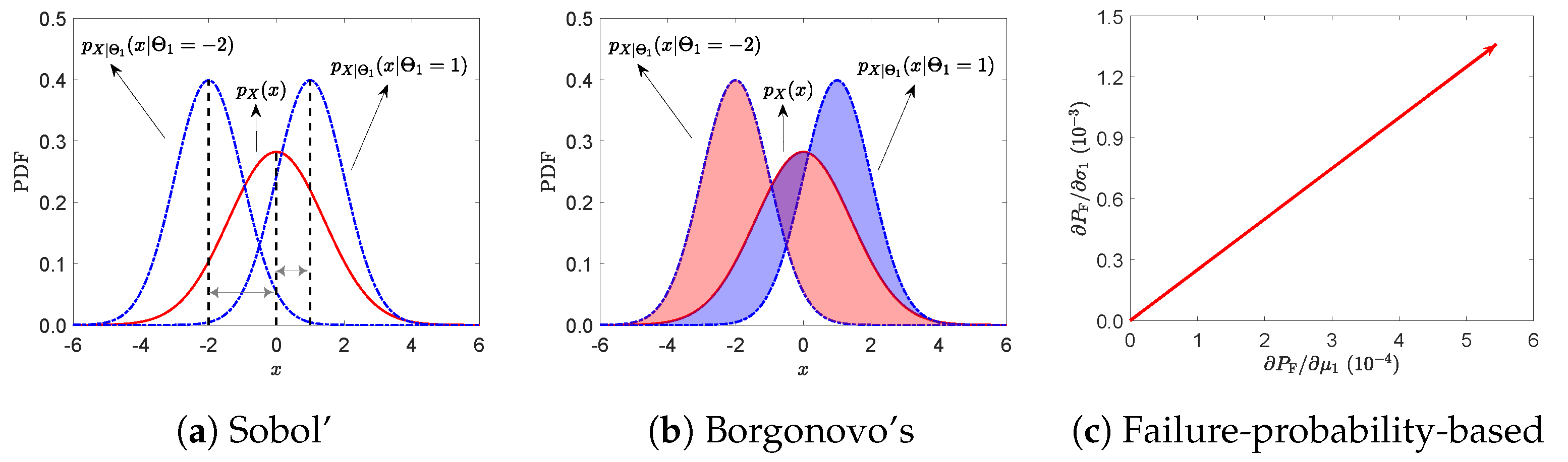
3. Review of Three Classical Global Sensitivity Indices

In this section, three classical global sensitivity indices (GSIs) are briefly revisited, including the variance-based GSI, the moment-independent GSI, and the failure-probability-based GSI. Moreover, to help illustrate the basic thinking behind the three GSIs, a simple toy model is considered in the following content, that is,

$$X={\mathrm{\Theta }}_1+{\mathrm{\Theta }}_2,$$

(10)

where ${\mathrm{\Theta }}_1$ and ${\mathrm{\Theta }}_2$ are independent normal variables, whose mean values are ${\mu }_1={\mu }_2=0$ and standard deviations are ${\sigma }_1={\sigma }_2=1$, in order. It is obvious that X follows the normal distribution $\mathcal{N}(0,\sqrt{2})$ with a mean value of 0 and a standard deviation equal to $\sqrt{2}$. Conditional $X|{\mathrm{\Theta }}_1$ and $X|{\mathrm{\Theta }}_2$ also follow the normal distribution $\mathcal{N}({\theta }_1,1)$ and $\mathcal{N}({\theta }_2,1)$, where ${\theta }_1$ and ${\theta }_2$ are certain realizations of ${\mathrm{\Theta }}_1$ and ${\mathrm{\Theta }}_2$, respectively.

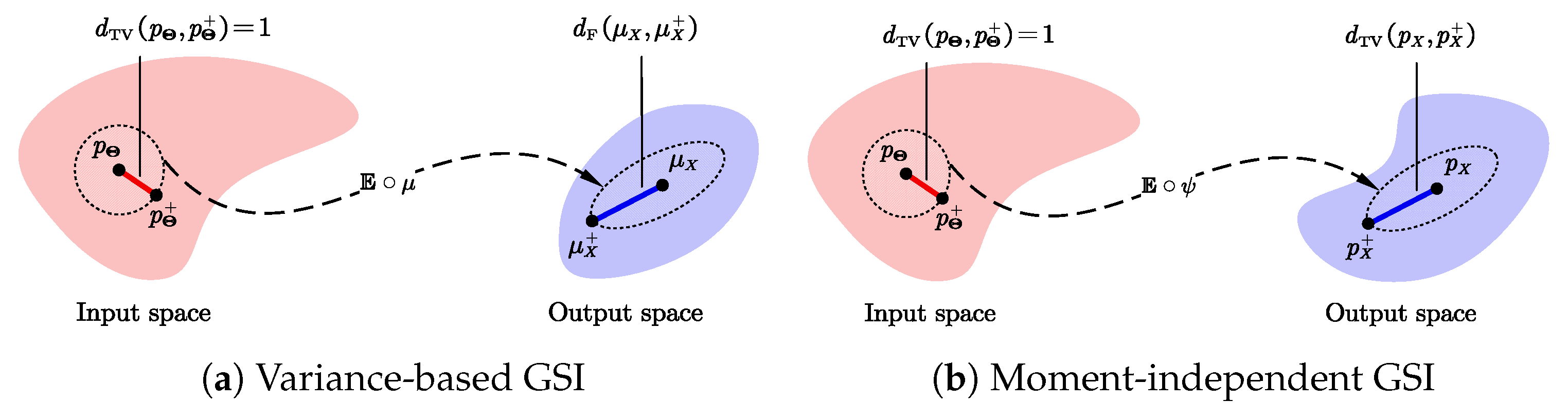
3.1. Variance-Based GSI

The variance-based GSI, also known as Sobol’ index [13,31], is one of the most popular GSIs in many disciplines [2]. The original Sobol’ index is defined on the assumption of independence of ${\mathrm{\Theta }}_i$’s, but it can be extended to dependent variables as well; see work in [14,32]. For the sake of simplicity, it is mentioned again that hereinafter only the independent case is considered.

The variance-based GSI is based on the contribution of basic input variables to the variance of the QoI, of which the first-order definition is given by

$$S_i^{\mathrm{S}}={\displaystyle \frac{\mathbb{D}\left[\mathbb{E}\left[X\right|{\mathrm{\Theta }}_i]\right]}{\mathbb{D}\left[X\right]}},S_i^{\mathrm{TS}}=1-{\displaystyle \frac{\mathbb{D}\left[\mathbb{E}\left[X\right|{\mathbf{\Theta }}_{\sim i}]\right]}{\mathbb{D}\left[X\right]}},i=1,2,\cdots ,s,$$

(11)

where ${\mathbf{\Theta }}_{\sim i}={({\mathrm{\Theta }}_1,\cdots ,{\mathrm{\Theta }}_{i-1},{\mathrm{\Theta }}_{i+1},\cdots ,{\mathrm{\Theta }}_s)}^{\top }$, $\mathbb{E}[·]$ and $\mathbb{D}[·]$ denote the expectation operator and the variance operator, respectively. $S_i^{\mathrm{S}}$ is called the main effect index, measuring the individual contribution of ${\mathrm{\Theta }}_i$ to the total variance $\mathbb{D}\left[X\right]$, while $S_i^{\mathrm{TS}}$ is called the total effect index, which not only shows the individual contribution of ${\mathrm{\Theta }}_i$ to the total variance $\mathbb{D}\left[X\right]$, but also reflects the interaction effect of ${\mathrm{\Theta }}_i$ with other input variables. It is obvious that $0\le S_i^{\mathrm{S}}\le S_i^{\mathrm{TS}}\le 1$. Moreover, the difference between $S_i^{\mathrm{TS}}$ and $S_i^{\mathrm{S}}$, i.e., $S_i^{\mathrm{TS}}-S_i^{\mathrm{S}}$ stands for the interaction effect of ${\mathrm{\Theta }}_i$, and it equals to zero if no interaction effect exits for ${\mathrm{\Theta }}_i$.

The intuition underlying the variance-based GSI is that, for each fixed ${\mathrm{\Theta }}_i={\theta }_i$, one can obtain a conditional output $X=g({\mathbf{\Theta }}_{\sim i},{\theta }_i)$, which is still a random variable but follows the conditional PDF $p_{X|{\mathrm{\Theta }}_i}\left(x\right|{\mathrm{\Theta }}_i={\theta }_i)$. Then, the mean value of this conditional output produces the inner integral in Equation (11), i.e.,

$$\begin{array}{cc}\hfill \mathbb{E}\left[X\right|{\mathrm{\Theta }}_i={\theta }_i]& ={\int }_{{\mathrm{\Omega }}_{{\mathbf{\Theta }}_{\sim i}}}g({\mathit{\theta }}_{\sim i},{\mathrm{\Theta }}_i={\theta }_i)p_{{\mathbf{\Theta }}_{\sim i}}\left({\mathit{\theta }}_{\sim i}\right)\mathrm{d}{\mathit{\theta }}_{\sim i}\hfill \\ \hfill & ={\int }_{{\mathrm{\Omega }}_X}x{p}_{X|{\mathrm{\Theta }}_i}\left(x\right|{\mathrm{\Theta }}_i={\theta }_i)\mathrm{d}x\stackrel{\mathrm{def}}{=}{g}_i\left({\theta }_i\right)\hfill \end{array}$$

(12)

and then we have $\mathbb{E}\left[X\right|{\mathrm{\Theta }}_i]=g_i\left({\mathrm{\Theta }}_i\right)$, considering now ${\mathrm{\Theta }}_i$ is a random variable (no longer fixed to ${\theta }_i$).

Let $\mathbb{E}\left[X\right]\stackrel{\mathrm{def}}{=}{\mu }_X$ and $\mathbb{D}\left[X\right]\stackrel{\mathrm{def}}{=}{\sigma }_X^2$. The ratio between the variance of $g_i\left({\mathrm{\Theta }}_i\right)$ that gives the outer integral in Equation (11), and the one of X is calculated by

$$\begin{array}{cc}\hfill S_i^{\mathrm{S}}& ={\displaystyle \frac{1}{{\sigma }_X^2}}{\int }_{{\mathrm{\Omega }}_{{\mathrm{\Theta }}_i}}{\left(g_i\left({\theta }_i\right)-{\mu }_X\right)}^2{p}_{{\mathrm{\Theta }}_i}\left({\theta }_i\right)\mathrm{d}{\theta }_i\hfill \\ \hfill & ={\displaystyle \frac{1}{{\sigma }_X^2}}{\int }_{{\mathrm{\Omega }}_{{\mathrm{\Theta }}_i}}{\left({\int }_{{\mathrm{\Omega }}_X}x{p}_{X|{\mathrm{\Theta }}_i}\left(x\right|{\mathrm{\Theta }}_i={\theta }_i)\mathrm{d}x-{\mu }_X\right)}^2{p}_{{\mathrm{\Theta }}_i}\left({\theta }_i\right)\mathrm{d}{\theta }_i,\hfill \end{array}$$

(13)

which is nothing but the main effect index $S_i^{\mathrm{S}}$.

The idea of fixing an input random variable in calculating the variance-based GSI is based on the pure thought that the variance of output can be reduced if uncertainty in this variable is eliminated [15]. Nevertheless, the variance-based GSI is somewhat questioned for the reason that the variance, i.e., the second-order statistics may not be sufficiently sensitive or informative [10]. Likewise, the variance-based GSI may lead to erroneous inferences or even opposite conclusions when the PDF of the QoI has multiple modes [23,33]. For instance, Borgonovo [23] has shown that the variance of a model output may even increase by setting a model input at a certain value, which is somewhat counter-intuitive.

With that said, the worth of the variance-based GSI is unquestioned, especially for its contribution to the variance-based reliability sensitivity analysis [2]. Specifically, the uniqueness of the variance-based GSI in reflecting the model structure will be illustrated in Section 5.3. The connection of the variance-based GSI with the moment-independent GSI will also be discussed hereinafter.

3.2. Moment-Independent GSI

The moment-independent GSI is defined on the entire distribution rather than a particular moment, and possibly the most popular one is Borgonovo’s $\delta$-index [15], which is defined as

$$\begin{array}{cc}\hfill S_i^{\delta }& ={\displaystyle \frac{1}{2}}\mathbb{E}\left[{\int }_{{\mathrm{\Omega }}_X}\left|p_{X|{\mathrm{\Theta }}_i}\left(x\right|{\mathrm{\Theta }}_i)-p_X\left(x\right)\right|\mathrm{d}x\right]\hfill \\ \hfill & ={\displaystyle \frac{1}{2}}{\int }_{{\mathrm{\Omega }}_{{\mathrm{\Theta }}_i}}{\int }_{{\mathrm{\Omega }}_X}\left|p_{X|{\mathrm{\Theta }}_i}\left(x\right|{\mathrm{\Theta }}_i={\theta }_i)-p_X\left(x\right)\right|p_{{\mathrm{\Theta }}_i}\left({\theta }_i\right)\mathrm{d}x\mathrm{d}{\theta }_i.\hfill \end{array}$$

(14)

Comparing Equation (13) with Equation (14), one can see that the expression of moment-independent GSI is very similar to that of variance-based GSI. Back to the thought of fixing an input random variable (e.g., ${\mathrm{\Theta }}_i={\theta }_i$), an intuitive understanding of the variance-based GSI and moment-independent GSI is as follows. Firstly, one can obtain the output PDF $p_X\left(x\right)$ when all input PDFs are set according to the corresponding distributions, which is mathematically expressed in Equation (9). If one of the input variables is fixed at a certain value, e.g., ${\mathrm{\Theta }}_i={\theta }_i$, then accordingly, the output PDF will become conditional by $p_{X|{\mathrm{\Theta }}_i}\left(x\right|{\mathrm{\Theta }}_i={\theta }_i)$. Thereupon, the effect of fixing an input variable at a certain value can be quantified by defining a distance between a quantity from the case of $p_X\left(x\right)$ and that of $p_{X|{\mathrm{\Theta }}_i}\left(x\right|{\mathrm{\Theta }}_i={\theta }_i)$. Hence, different distances will lead to different definitions of GSI. For the variance-based GSI, the Bregman distance is considered, while for the moment-independent GSI, the distribution distance is taken into account. Specifically, the variance-based GSI is defined by calculating the mean of Bregman distances by Equation (13), while the moment-independent GSI is based on the mean of distribution distances (the total variation distance) by Equation (14).

A visual interpretation is presented in Figure 1a,b. To some extent, it is seen clearly that the basic idea (concise but creative) of the variance-based GSI and the moment-independent GSI is almost consistent.

3.3. Failure-Probability-Based GSI

The failure probability is of paramount significance in measuring the safety of a system. However, it may be highly sensitive to basic input random variables and, in particular, may vary considerably with respect to different distribution parameters, e.g., mean values or standard deviations [18]. To this end, it is essential to evaluate the failure-probability-based GSI, which is commonly defined by [17]

$$S_{i,j}^{\mathrm{F}}={\displaystyle \frac{\partial P_{\mathrm{F}}\left(\mathit{\xi }\right)}{\partial {\xi }_{i,j}}},i=1,2,\cdots ,s,j=1,2,\cdots ,s_i,$$

(15)

where ${\xi }_{i,j}$ is the j-th distribution parameter for the i-th input random variable ${\mathrm{\Theta }}_i$, and $P_{\mathrm{F}}$ is the failure probability calculated by

$$P_{\mathrm{F}}\left(\mathit{\xi }\right)={\int }_{{\mathrm{\Omega }}_{\mathrm{F}}}{p}_X(x;\mathit{\xi })\mathrm{d}x,$$

(16)

where ${\mathrm{\Omega }}_{\mathrm{F}}$ stands for the failure domain corresponding to the failure criteria based on strength, deformation, displacement, energy, etc. Specifically, if the function $g(·)$ in Equation (1) is the performance function [34], the failure domain can be defined as ${\mathrm{\Omega }}_{\mathrm{F}}\subseteq {\mathrm{\Omega }}_X:x=g\left(\mathit{\theta }\right)<0$.

Alternatively, the failure-probability-based GSI can be expressed by combing Equations (15) and (16) and by exchanging the order of differentiation and integration in Assumption (a) in Section 2, i.e.,

$$S_{i,j}^{\mathrm{F}}={\int }_{{\mathrm{\Omega }}_{\mathrm{F}}}{\displaystyle \frac{\partial p_X(x;\mathit{\xi })}{\partial {\xi }_{i,j}}}\mathrm{d}x.$$

(17)

An illustration of the failure-probability-based GSI is drawn in Figure 1c, with consideration given to the toy model in Equation (10), where the failure domain is defined by $x>5$.

Unlike variance-based GSI or moment-independent GSI, failure-probability-based GSI for each ${\mathrm{\Theta }}_i$ may have more than one value, i.e., $S_i^{\mathrm{F}}={(S_{i,1}^{\mathrm{F}},\cdots ,S_{i,s_i}^{\mathrm{F}})}^{\top }$, whose dimension is dependent on the number of distribution parameters of ${\mathrm{\Theta }}_i$. In addition, $S_{i,j}^{\mathrm{F}}$ is not guaranteed to be positive. For convenience in future discussions, we define $\parallel S_i^{\mathrm{F}}{\parallel }_{\infty }$ as a characteristic measure of the failure-probability-based GSI, where ${\parallel ·\parallel }_{\infty }$ is the ∞-norm.

3.4. Objectives of This Research and Adopted Methods

This paper is mainly with a focus on the following three aspects: (1) some valuable properties of a newly developed Fréchet-derivative-based GSI (Fre-GSI) in [10], which will be introduced in the following section; (2) a unified description from a functional perspective of the three GSIs and the Fre-GSI; (3) some practical links of the Fre-GSI with the three GSIs. For the sake of simplicity, in Section 5, we will study three examples with analytical solutions and one engineering application that can be computed numerically. These results can also be reproduced via, e.g., the well-known Monte Carlo simulation (MCS) [14,18], which is familiar to the reader. Additionally, for moment-independent GSI and Fre-GSI, the kernel density estimation (KDE) can be adopted to estimate the unconditional and conditional PDFs of the QoI [7,16]. It should be emphasized that any efficient numerical algorithms for calculating the above GSIs are welcomed, see [14,16,18,35,36]. However, the current study aims to provide a clear and novel picture of the four GSIs in a relatively simple way, so using analytical or partially analytical examples, which can be verified numerically by adopting the MCS and KDE, is only for the convenience of discussion.

4. Fréchet-Derivative-Based GSI

4.1. Definition of the Fréchet-Derivative-Based GSI and Its Parametric Expression

As mentioned above, an ideal GSI is expected to not only measure the importance of each model input but also characterize the direction of this importance. These two features will undoubtedly help to reflect the basic physical mechanisms of stochastic parametric models. In probability theory, it is well known that the PDF of the QoI can be uniquely defined if the studied stochastic model is well-posed and the PDF of model inputs is also precisely determined. This fact is also known as the rule of change of random variables (CRV) [37], which can be compactly expressed in an operator form; see the formula in Equation (9). In this sense, a natural GSI in terms of stochastic models can be heuristically defined as an extension of the “partial derivative” of a function in the context of the operator of uncertainty propagation (UP), as shown in Figure 2. From the perspective of functional analysis, the Fréchet derivative can perform this task in theory. In summary, based on the conceptual idea of the Fréchet derivative, the Fréchet-derivative-based GSI (Fre-GSI) can serve as a natural GSI that may be more compatible with stochastic models.

The Fre-GSI ${\mathcal{F}}_i$ for the i-th parameter ${\mathrm{\Theta }}_i$ is defined by [10]

$$\underset{{∥\mathrm{\delta }{p}_{{\Theta }_i}∥}_V\to 0}{lim}{\displaystyle \frac{{∥\psi \left[p_{\mathbf{\Theta }}+\delta p_{{\mathrm{\Theta }}_i}\right]-\psi \left[p_{\mathbf{\Theta }}\right]-{\mathcal{F}}_i\delta p_{{\mathrm{\Theta }}_i}∥}_W}{{∥\delta p_{{\mathrm{\Theta }}_i}∥}_V}}=0,$$

(18)

where $\delta p_{{\mathrm{\Theta }}_i}$ is a small perturbation of $p_{{\mathrm{\Theta }}_i}$ satisfying $\int \delta p_{{\mathrm{\Theta }}_i}=0$ and $\delta p_{{\mathrm{\Theta }}_i}>-p_{\mathbf{\Theta }}$. ${\parallel ·\parallel }_W$ and ${\parallel ·\parallel }_V$ are two appropriately equipped norms (e.g., half of the ${\ell }_1$-norm) on the Banach spaces W and V of $p_X$ and $p_{{\mathrm{\Theta }}_i}$, respectively. It should be noted that, here, the Fre-GSI is defined by the Fréchet derivative of $\psi$, and since $\psi$ is a linear operator, the Fréchet derivative of $\psi$ is exactly itself [10].

If $p_{\mathbf{\Theta }}\left(\mathit{\theta }\right)$ is a parametric distribution with certain distribution parameters $\mathbf{\xi }$, i.e., $p_{\mathbf{\Theta }}(\mathit{\theta };\mathit{\xi })$, then the parametric form of the Fre-GSI can be derived as [10]

$${\mathcal{F}}_{i,j}(x;\mathit{\xi })={\displaystyle \frac{\partial p_X(x;\mathit{\xi })}{\partial {\xi }_{i,j}}}/∥{\displaystyle \frac{\partial p_{\mathbf{\Theta }}(\mathit{\theta };\mathit{\xi })}{\partial {\xi }_{i,j}}}∥,$$

(19)

where $\parallel ·\parallel$ is defined by ${\displaystyle \frac{1}{2}}\int \left|p\right|$. Based on the assumption of independence of $\mathbf{\Theta }$, the denominator in Equation (19) (the norm term) can be further simplified to $∥\partial p_{{\mathrm{\Theta }}_i}({\theta }_i;{\mathit{\xi }}_i)/\partial {\xi }_{i,j}∥$. In addition, it is obvious that ${\mathcal{F}}_{i,j}(x;\mathit{\xi })$ satisfies

$${\int }_{{\mathrm{\Omega }}_X}{\mathcal{F}}_{i,j}(x;\mathit{\xi })\mathrm{d}x=0$$

(20)

due to the fact that ${\int }_{{\mathrm{\Omega }}_X}{p}_X(x;\mathit{\xi })\mathrm{d}x=1$. In the following, x and $\mathit{\xi }$ in ${\mathcal{F}}_{i,j}(x;\mathit{\xi })$ are omitted for simplicity.

Compared with the variance-based GSI in Equation (13), the moment-independent GSI in Equation (14), and the failure-probability-based GSI in Equation (15), the Fre-GSI in Equation (19) is not a scalar but a function of x. In this sense, the Fre-GSI reflects the sensitivity of each realization of X to inputs.

Computing the Fre-GSI in Equation (19) mainly includes two steps: (1) Estimate the PDF of X in terms of $\mathit{\xi }$ and the perturbed PDF of X in terms of ${\mathit{\xi }}^{*}$. This can be carried out using, for example, moment-based methods [38], kernel density estimation [22], probability density evolution method [39], etc. (2) Approximate the derivative of PDF of X via finite difference methods [10], i.e., ${\displaystyle \frac{\partial p_X(x;\mathit{\xi })}{\partial {\xi }_{i,j}}}\approx {\displaystyle \frac{p_X^{*}(x;{\mathit{\xi }}^{*})-p_X(x;\mathit{\xi })}{{\mathit{\xi }}^{*}-\mathit{\xi }}}$. The denominator in Equation (19) (i.e., the norm term) can be computed analytically or numerically [10]. Moreover, by Equations (9) and (19), we have

$$\begin{array}{cc}\hfill {\mathcal{F}}_{i,j}(x;\mathit{\xi })& ={\displaystyle \frac{\partial \left[\psi \circ p_{\mathbf{\Theta }}(\mathit{\theta };\mathit{\xi })\right]}{\partial {\xi }_{i,j}}}/∥{\displaystyle \frac{\partial p_{\mathbf{\Theta }}(\mathit{\theta };\mathit{\xi })}{\partial {\xi }_{i,j}}}∥\hfill \\ \hfill & =\psi \circ {\displaystyle \frac{\partial p_{\mathbf{\Theta }}(\mathit{\theta };\mathit{\xi })}{\partial {\xi }_{i,j}}}/∥{\displaystyle \frac{\partial p_{\mathbf{\Theta }}(\mathit{\theta };\mathit{\xi })}{\partial {\xi }_{i,j}}}∥,\hfill \end{array}$$

(21)

which indicates that the parametric expression of the Fre-GSI is the result of the UP operator acting on the unitized derivative of the input distribution with respect to the distribution parameter [40]. Furthermore, the geometric meaning of the Fre-GSI is the variation of the input distribution as the “direction” and “size” of the points (vectors) in the abstract space after the change of the state of the system.

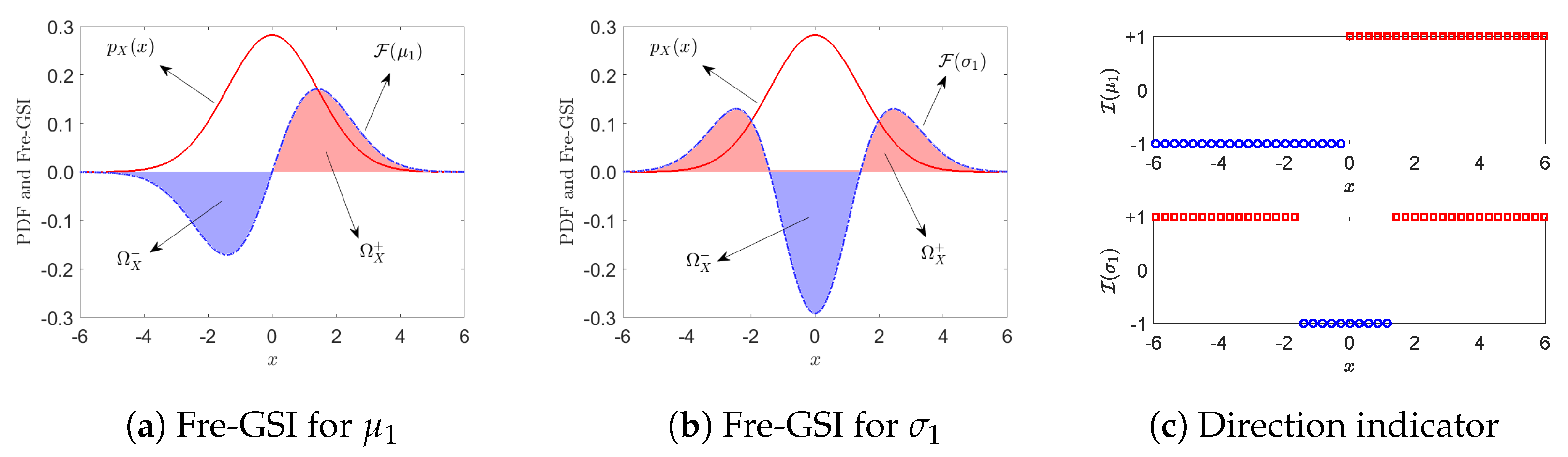
4.2. Importance Measure and Direction Indicator of the Fre-GSI

Two practical quantities can be generated from the Fre-GSI [29], i.e., the importance measure defined by

$$S_{i,j}^{\mathcal{F}}=∥{\mathcal{F}}_{i,j}∥,i=1,2,\cdots ,s;j=1,2,\cdots ,s_i,$$

(22)

and the direction indicator defined by

$${\mathcal{I}}_{i,j}=\mathrm{sgn}\left({\mathcal{F}}_{i,j}\right),$$

(23)

where $\mathrm{sgn}\left(A\right)$ is the sign function, viz., $\mathrm{sgn}\left(A\right)=A/\left|A\right|$ for $A\ne 0$ and $\mathrm{sgn}\left(A\right)=0$ for $A=0$. Regarding the direction indicator, it is convenient to divide ${\mathrm{\Omega }}_X$ into a positive region ${\mathrm{\Omega }}_X^{+}$, a negative region ${\mathrm{\Omega }}_X^{-}$, and a zero region ${\mathrm{\Omega }}_X^0$ based on the direction indicator ${\mathcal{I}}_{i,j}$, i.e.,

$${\mathrm{\Omega }}_X^{+}:x·I\left({\mathcal{I}}_{i,j}=+1\right),{\mathrm{\Omega }}_X^{-}:x·I\left({\mathcal{I}}_{i,j}=-1\right),{\mathrm{\Omega }}_X^0:x·I\left({\mathcal{I}}_{i,j}=0\right),$$

(24)

where $I\left(A\right)=1$ if and only if A holds true, otherwise $I\left(A\right)=0$.

As for the importance measure, there are two important properties: (Property 1) $0\le S_{i,j}^{\mathcal{F}}\le 1$; (Property 2) $S_{i,j}^{\mathcal{F}}=1$ holds when $s=1$ and $g(·)$ in Equation (1) is monotonic. For the sake of lengthiness herein, the proofs of Property 1 and Property 2 are given in Appendix A.1 and Appendix A.2, respectively. One can also find a similar proof of Property 2 for the study of the moment-independent GSI in [16] (p. 422). Additionally, similar to the failure-probability-based GSI, the importance measure based on the Fre-GSI for each ${\mathrm{\Theta }}_i$ may contain more than just one value, i.e., $S_i^{\mathcal{F}}={(S_{i,1}^{\mathcal{F}},\cdots ,S_{i,s_i}^{\mathcal{F}})}^{\top }$. Hereinafter, the mentioned Fre-GSI is specifically referred to as the parametric Fre-GSI in Equation (19). For this reason, ${∥S_i^{\mathcal{F}}∥}_{\infty }$ is utilized for the following discussion.

An illustration of the Fre-GSI and its corresponding direction indicator is presented in Figure 3 by taking the toy model in Equation (10) for example. Notably, the sum of colored areas above (or below) the X-axis is exactly the importance measure based on the Fre-GSI.

4.3. Links of the Fréchet-Derivative-Based GSI with the Three Classical GSIs

As previously discussed, whether it is the variance-based GSI, moment-independent GSI, failure-probability-based GSI or the Fre-GSI, it can be seen that a practical GSI for the GSA is supposed to satisfy the instructive concept stated in [12] that “the study of how uncertainty in the output of a model (numerical or otherwise) can be apportioned to different sources of uncertainty in the model input”. Thus, quantification of different QoIs (output) measured by different means (how) forms the connotation of different GSIs. Based on this understanding, a functional perspective is presented in Figure 4 to illustrate the above four GSIs.

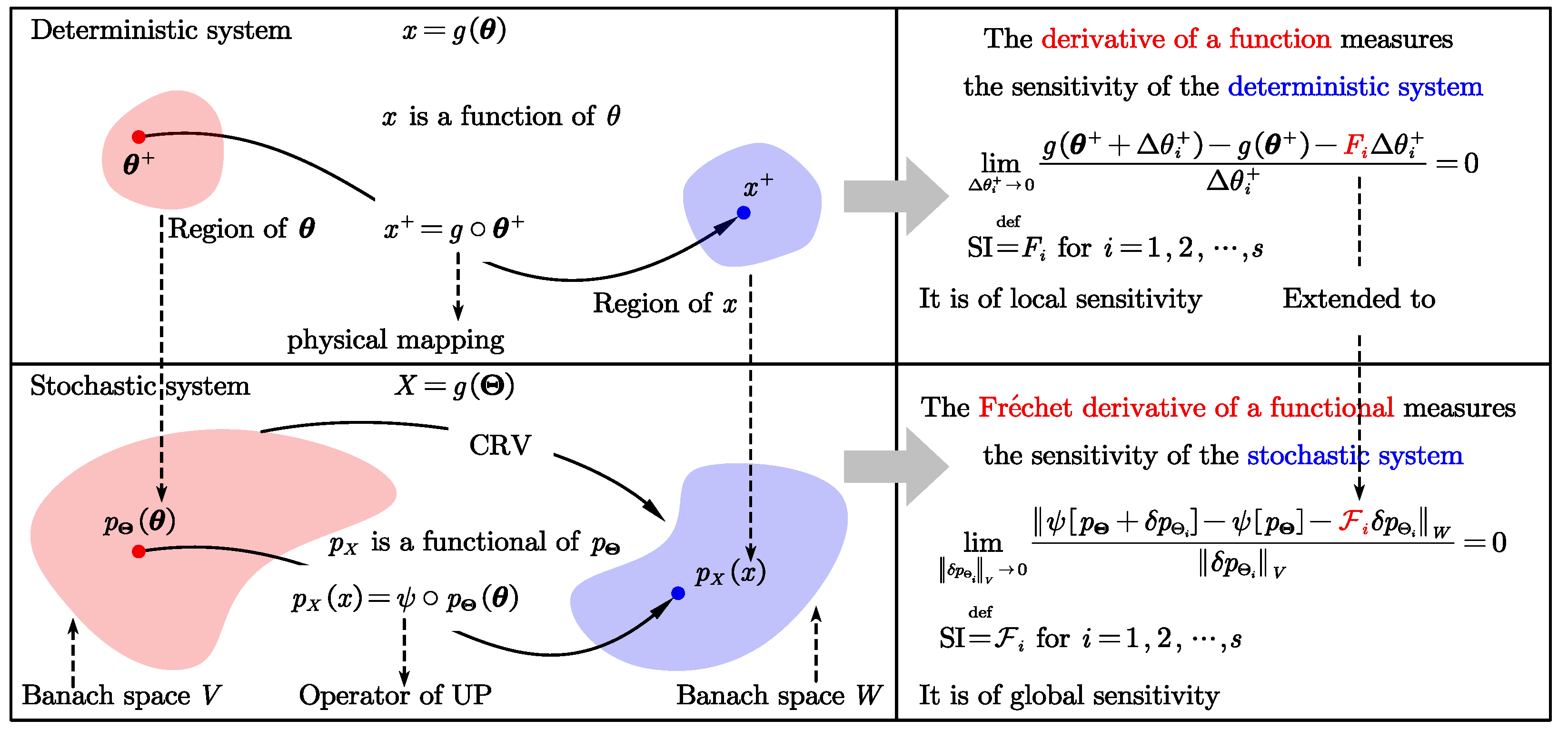
4.3.1. On the Concept of the Output from a Functional Perspective

Specifically, in Figure 4, the input space stretched by the PDF of inputs, i.e., $p_{\mathbf{\Theta }}(\mathit{\theta };\mathit{\xi })$, is the same for four classes of GSIs. However, the output space is different: for the variance-based GSI (Figure 4a), the conditional mean value of X is of interest; for the failure-probability-based GSI (Figure 4c), the failure probability of X is concerned; while for the moment-independent GSI in Figure 4b (and Fre-GSI in Figure 4d), the conditional PDF of X is taken into account.

Consequently, the mappings from the input space to different output spaces can be determined by specific operators: (1) for the variance-based GSI, we define that ${\mu }_X=\mu \circ p_{\mathrm{\Theta }}$; (2) for the failure probability of X, and by introducing Equation (16) to Equation (9), it leads to $P_{\mathrm{F}}=\varphi \circ \psi \circ p_{\mathbf{\Theta }}$, where $\varphi$ is the operator for $P_{\mathrm{F}}=\varphi \circ p_X(x;\mathit{\xi })$; (3) for the PDF of X, the UP operator $\psi$ has been defined previously in Equation (9).

4.3.2. On the Concept of the How from a Functional Perspective

Recall the definition of variance-based GSI and moment-independent GSI, the thought of fixing an input random variable ${\mathrm{\Theta }}_i$ to a certain value ${\overline{\theta }}_i$ will lead to a “collapse” of the PDF of $\mathbf{\Theta }$, i.e.,

$$p_{\mathbf{\Theta }}\left(\mathit{\theta }\right)\to p_{\mathbf{\Theta }}^{+}\left(\mathit{\theta }\right)\stackrel{\mathrm{def}}{=}\prod _{k=1,k\ne i}^s{p}_{{\mathrm{\Theta }}_k}\left({\theta }_k\right){\delta }_{\mathrm{D}}({\theta }_i-{\overline{\theta }}_i),$$

(25)

and the corresponding total variation distance between $p_{\mathbf{\Theta }}$ and $p_{\mathbf{\Theta }}^{+}$ is

$$\begin{array}{cc}\hfill d_{\mathrm{TV}}\left(p_{\mathbf{\Theta }},p_{\mathbf{\Theta }}^{+}\right)& ={\displaystyle \frac{1}{2}}{\int }_{{\mathrm{\Omega }}_{\mathbf{\Theta }}}\left|p_{\mathbf{\Theta }}^{+}-p_{\mathbf{\Theta }}\right|\mathrm{d}\mathit{\theta }\hfill \\ \hfill & ={\displaystyle \frac{1}{2}}{\int }_{{\mathrm{\Omega }}_{{\mathrm{\Theta }}_i}}\left|{\delta }_{\mathrm{D}}\left({\theta }_i-{\overline{\theta }}_i\right)-p_{{\mathrm{\Theta }}_i}\left({\theta }_i\right)\right|\mathrm{d}{\theta }_i=1,\hfill \end{array}$$

(26)

which means that the input space undergoes a unit-volume change when the i-th random variable collapses to a deterministic value. Let $p_X$ and $p_X^{+}$ be the PDFs of X, ${\mu }_X$ and ${\mu }_X^{+}$ be the mean values of X, with respect to $p_{\mathbf{\Theta }}$ and $p_{\mathbf{\Theta }}^{+}$. The changes in the output spaces can be defined by $d_{\mathrm{F}}\left({\mu }_X,{\mu }_X^{+}\right)$ and $d_{\mathrm{TV}}\left(p_X,p_X^{+}\right)$ in terms of the variance-based GSI and the moment-independent GSI [7], respectively, where $d_{\mathrm{F}}(a,b)$ is the Bregman distance, i.e., the squared Euclidean distance defined by $d_{\mathrm{F}}(a,b)={(a-b)}^2$. Then, the variance-based GSI in Equation (13) and the moment-independent GSI in Equation (14) can be rewritten by

$$S_i^{\mathrm{S}}={\displaystyle \frac{1}{{\sigma }_X^2}}\mathbb{E}\left[{\displaystyle \frac{d_{\mathrm{F}}\left({\mu }_X,{\mu }_X^{+}\right)}{d_{\mathrm{TV}}\left(p_{\mathbf{\Theta }},p_{\mathbf{\Theta }}^{+}\right)}}\right],S_i^{\delta }=\mathbb{E}\left[{\displaystyle \frac{d_{\mathrm{TV}}\left(p_X,p_X^{+}\right)}{d_{\mathrm{TV}}\left(p_{\mathbf{\Theta }},p_{\mathbf{\Theta }}^{+}\right)}}\right],$$

(27)

where the expectation is calculated by taking the average of values in the dashed regions in Figure 4a,b.

Similarly, considering that the distribution parameter has a small perturbation from ${\xi }_{i,j}$ to ${\xi }_{i,j}^{*}$, the input PDF is changed from $p_{\mathbf{\Theta }}$ to $p_{\mathbf{\Theta }}^{*}$. Correspondingly, the failure probability and the PDF of X are changed to $P_{\mathrm{F}}^{*}$ and $p_X^{*}$, respectively. By finite difference methods, the failure-probability-based GSI in Equation (15) and the importance measure of the Fre-GSI in Equation (22) can be rewritten by

$$S_{i,j}^{\mathrm{F}}={\displaystyle \frac{P_{\mathrm{F}}^{*}-P_{\mathrm{F}}}{{\xi }_{i,j}^{*}-{\xi }_{i,j}}},S_{i,j}^{\mathcal{F}}={\displaystyle \frac{d_{\mathrm{TV}}\left(p_X,p_X^{*}\right)}{d_{\mathrm{TV}}\left(p_{\mathbf{\Theta }},p_{\mathbf{\Theta }}^{*}\right)}}.$$

(28)

Now, the physical significance of the four GSIs is abundantly clear. Analogous to the deformation gradient in continuum mechanics, the GSIs in Equations (27) and (28) reflect the average rate and the rate of volume change (for the Fre-GSI, it is actually the absolute rate of volume change) from the input space to the output space, when there is a specific perturbation in the input PDF. More specifically, for the variance-based GSI and the moment-independent GSI, the perturbation is set by fixing an input random variable to a deterministic value, while for the failure-probability-based GSI and the Fre-GSI, it is to make a distribution parameter slightly perturbed.

Additionally, assume the distribution parameters of ${\mathrm{\Theta }}_i$ are uniquely determined by the mean value ${\mu }_i$ and the standard deviation ${\sigma }_i$ of ${\mathrm{\Theta }}_i$, i.e., $p_{{\mathrm{\Theta }}_i}({\theta }_i;{\mu }_i,{\sigma }_i)$. When ${\mathrm{\Theta }}_i$ collapses to ${\overline{\theta }}_i$, the PDF of ${\mathrm{\Theta }}_i$ turns out to be ${\delta }_{\mathrm{D}}({\theta }_i-{\overline{\theta }}_i)$, which can be regarded as $p_{{\mathrm{\Theta }}_i}({\theta }_i;{\mu }_i\to {\overline{\theta }}_i,{\sigma }_i\to 0)$. A specific example is that if ${\mathrm{\Theta }}_i$ is a normal random variable with mean value ${\mu }_i$ and standard deviation ${\sigma }_i$, the PDF of ${\mathrm{\Theta }}_i$ can be expressed as the limiting form of ${\displaystyle \frac{1}{\sqrt{2\pi }{\sigma }_i}}exp\{-{\displaystyle \frac{{({\theta }_i-{\mu }_i)}^2}{2{\sigma }_i^2}}\}$ with ${\mu }_i\to {\overline{\theta }}_i$ and ${\sigma }_i\to 0$ when ${\mathrm{\Theta }}_i$ collapses to ${\overline{\theta }}_i$.

4.3.3. Links Between the Fre-GSI to the Three Classical GSIs

The derivative of the variance-based GSI with respect to the distribution parameter can be derived from the Fre-GSI (the proof is given in Appendix A.3), i.e.,

$${\displaystyle \frac{\partial S_i^{\mathrm{S}}}{\partial {\xi }_{i,j}}}=-∥{\displaystyle \frac{\partial p_{{\mathrm{\Theta }}_i}({\theta }_i;{\mathit{\xi }}_i)}{\partial {\xi }_{i,j}}}∥S_i^{\mathrm{S}}·{\int }_{{\mathrm{\Omega }}_X}{\displaystyle \frac{{(x-{\mu }_X)}^2}{{\sigma }_X^2}}{\mathcal{F}}_{i,j}\mathrm{d}x+{\int }_{{\mathrm{\Omega }}_{{\mathrm{\Theta }}_i}}{s}_i^{\mathrm{S}}({\theta }_i;{\mathit{\xi }}_i){\displaystyle \frac{\partial p_{{\mathrm{\Theta }}_i}}{\partial {\xi }_{i,j}}}\mathrm{d}{\theta }_i\stackrel{\mathrm{def}}{=}\mathrm{EQ}1,$$

(29)

where

$$s_i^{\mathrm{S}}({\theta }_i;{\mathit{\xi }}_i)={\displaystyle \frac{1}{{\sigma }_X^2\left({\mathit{\xi }}_i\right)}}{\left({\int }_{{\mathrm{\Omega }}_X}x{p}_{X|{\mathrm{\Theta }}_i}\left(x\right|{\mathrm{\Theta }}_i={\theta }_i)\mathrm{d}x-{\mu }_X\left({\mathit{\xi }}_i\right)\right)}^2$$

(30)

is assumed to be known. Actually, $s_i^{\mathrm{S}}({\theta }_i;{\mathit{\xi }}_i)$ is a one-dimensional function of ${\theta }_i$, which can be computed by regression methods as suggested in [41].

Similarly, the upper bound of the absolute value of the derivative of the moment-independent GSI with respect to the distribution parameter can be given from the Fre-GSI by

$$\left|{\displaystyle \frac{\partial S_i^{\delta }}{\partial {\xi }_{i,j}}}\right|\le ∥{\displaystyle \frac{\partial p_{\mathbf{\Theta }}(\mathit{\theta };\mathit{\xi })}{\partial {\xi }_{i,j}}}∥·S_{i,j}^{\mathcal{F}}+∥{\displaystyle \frac{\partial p_{{\mathrm{\Theta }}_i}({\theta }_i;{\mathit{\xi }}_i)}{\partial {\xi }_{i,j}}}∥\stackrel{\mathrm{def}}{=}\mathrm{UB}2,$$

(31)

which provides convenience to learn the robustness of $S_i^{\delta }$ with respect to the basic distribution parameters without estimating $S_i^{\delta }$. The proof is given in Appendix A.4.

A practical conversion from the Fre-GSI to the failure-probability-based GSI reads

$$S_{i,j}^{\mathrm{F}}=∥{\displaystyle \frac{\partial p_{\mathbf{\Theta }}(\mathit{\theta };\mathit{\xi })}{\partial {\xi }_{i,j}}}∥·{\int }_{{\mathrm{\Omega }}_{\mathrm{F}}}{\mathcal{F}}_{i,j}\mathrm{d}x\stackrel{\mathrm{def}}{=}\mathrm{EQ}3,$$

(32)

which means the failure-probability-based GSI is proportional to the integral of the Fre-GSI in the failure domain, where the proportional coefficient is exactly the norm term in the Fre-GSI. Additionally, an inequality between $\left|S_{i,j}^{\mathrm{F}}\right|$ and $S_{i,j}^{\mathcal{F}}$ can be derived by

$$\left|S_{i,j}^{\mathrm{F}}\right|\le ∥{\displaystyle \frac{\partial p_{\mathbf{\Theta }}(\mathit{\theta };\mathit{\xi })}{\partial {\xi }_{i,j}}}∥·S_{i,j}^{\mathcal{F}}\stackrel{\mathrm{def}}{=}\mathrm{UB}3,$$

(33)

where the proof of Equations (32) and (33) is available in Appendix A.5. From Equation (33), it is interesting to find that the upper bound of the absolute value of $S_{i,j}^{\mathrm{F}}$ is independent of the failure criterion. Hence, by Equation (33), the decision-maker can flexibly know in advance which parameters may be influential on the failure probability, without calculating the failure probability in terms of a certain criterion of failure.

5. Test Examples

The following four examples are studied to verify the proposed links of the Fre-GSI with the variance-based, moment-independent, and failure-probability-based GSIs. In particular, these examples are also designed to investigate the specific performance of the four GSIs. Specifically, Example 1 aims to study whether the four GSIs are able to effectively distinguish between two similar but different systems; Example 2 examines whether the four GSIs are sensitive to the distribution parameters for nonlinear systems; Example 3 is to study the impact of the increasing model size on the four GSIs, while Example 4 is to validate the specific capabilities of the four GSIs in real engineering practices.

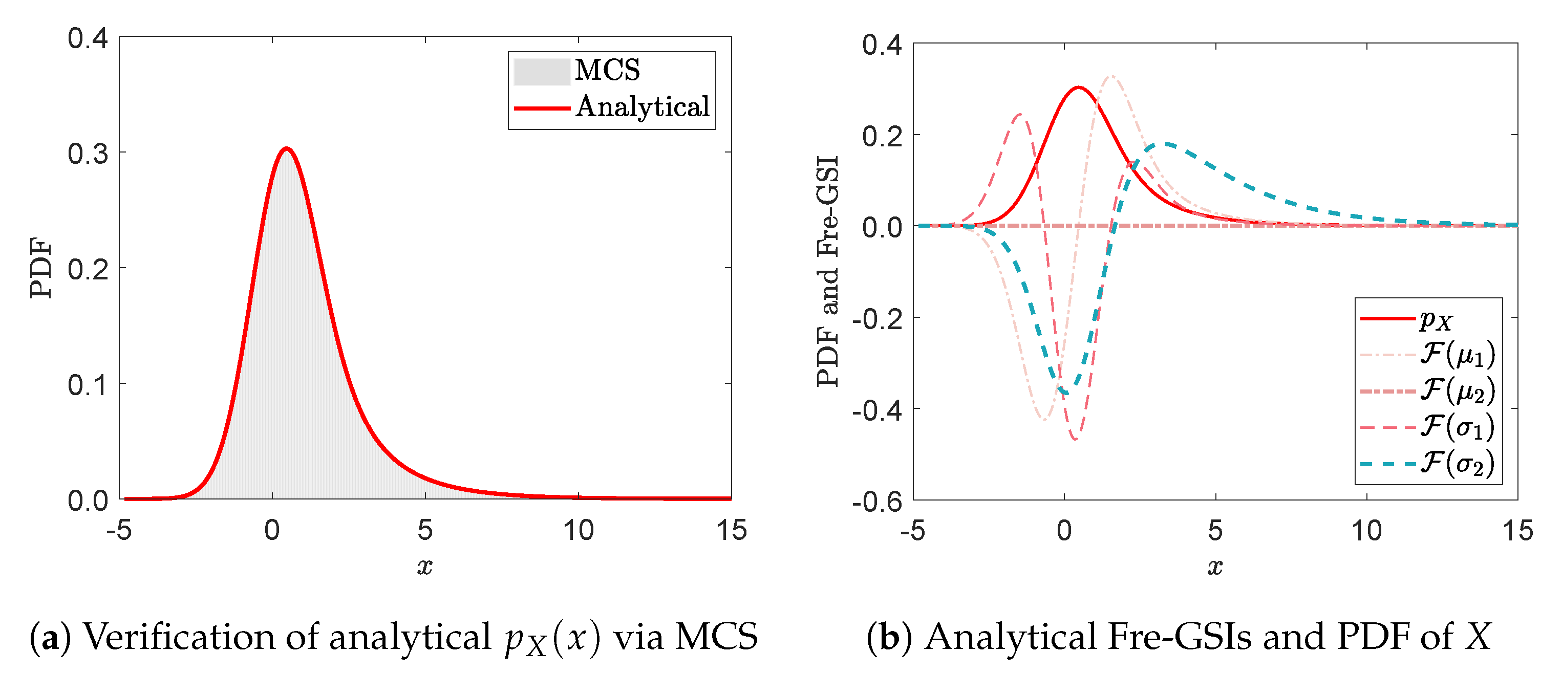
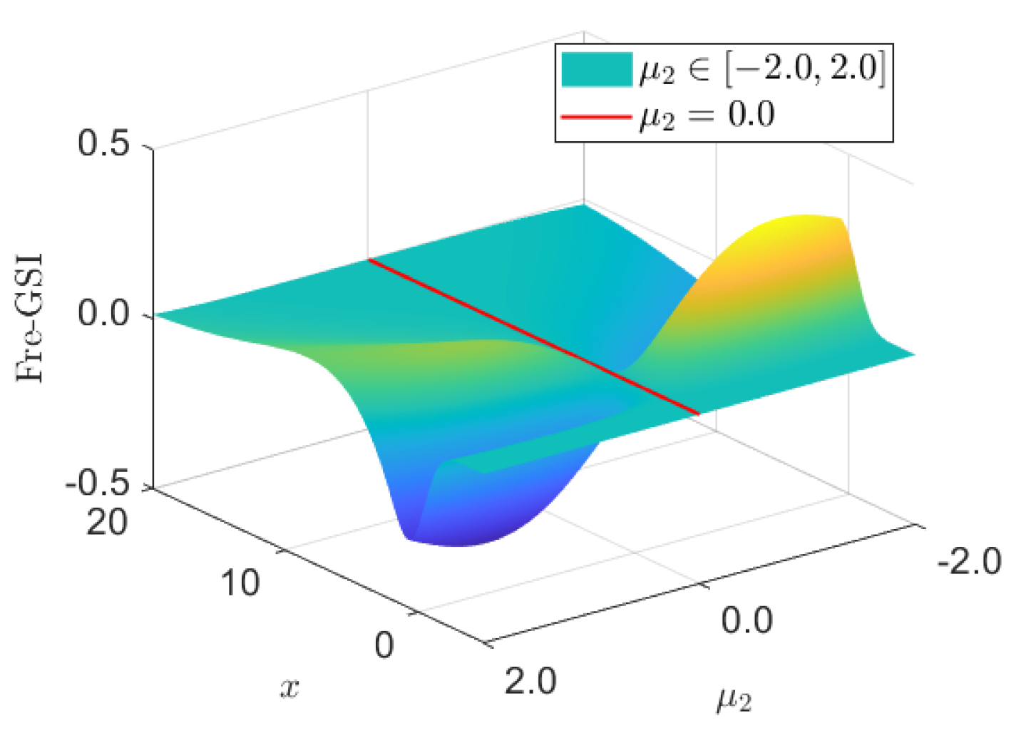
5.1. Example 1: A Similar Toy Model

We first study a toy model that is very similar to the one in Equation (10), i.e.,

$$X={\mathrm{\Theta }}_1-{\mathrm{\Theta }}_2,$$

(34)

where ${\mathrm{\Theta }}_1$ and ${\mathrm{\Theta }}_2$ are i.i.d. standard normal random variables. The unconditional X follows $\mathcal{N}(0,\sqrt{2})$ in the same way, and conditional $X|{\mathrm{\Theta }}_1$ and $X|{\mathrm{\Theta }}_2$ follow $\mathcal{N}({\theta }_1,1)$ and $\mathcal{N}(-{\theta }_2,1)$, respectively. Thus, theoretical solutions of the four GSIs can be calculated by definition and are listed in

Table 1. The theoretical solutions of the four GSIs (Example 1).

${\mathbf{\Theta }}_{\mathit{i}}$	${\mathit{\xi }}_{\mathit{i},\mathit{j}}$	${\mathit{S}}_{\mathit{i}}^{\mathbf{S}}$	$\mathit{\partial }{\mathit{S}}_{\mathit{i}}^{\mathbf{S}}/\mathit{\partial }{\mathit{\xi }}_{\mathit{i},\mathit{j}}$	EQ1	${\mathit{S}}_{\mathit{i}}^{\mathit{\delta }}$	$\mathit{\partial }{\mathit{S}}_{\mathit{i}}^{\mathit{\delta }}/\mathit{\partial }{\mathit{\xi }}_{\mathit{i},\mathit{j}}$	UB2	${\mathit{S}}_{\mathit{i},\mathit{j}}^{\mathbf{F}}$	EQ3	UB3	${\mathit{S}}_{\mathit{i},\mathit{j}}^{\mathcal{F}}$
${\mathrm{\Theta }}_1$	${\mu }_1$	$0.500$	$0.000$	$0.000$	$0.306$	$0.000$	$0.681$	${0.220 }^{†}$	${0.220 }^{†}$	$0.282$	$0.707$
								${0.005 }^{‡}$	${0.005 }^{‡}$
	${\sigma }_1$		$0.500$	$0.500$		$0.261$	$0.726$	${0.110 }^{†}$	${0.110 }^{†}$	$0.242$	$0.500$
								${0.010 }^{‡}$	${0.010 }^{‡}$
${\mathrm{\Theta }}_2$	${\mu }_2$	$0.500$	$0.000$	$0.000$	$0.306$	$0.000$	$0.681$	$-{0.220 }^{‡}$	$-{0.220 }^{†}$	$0.282$	$0.707$
								$-{0.005 }^{‡}$	$-{0.005 }^{‡}$
	${\sigma }_2$		$0.500$	$0.500$		$0.261$	$0.726$	${0.110 }^{†}$	${0.110 }^{†}$	$0.242$	$0.500$
								${0.010 }^{‡}$	${0.010 }^{‡}$

Note: The superscripts ^† and ^‡ stand for the failure domains defined as $x>1$ and $x>4$, respectively.

, where EQ1 in Equation (29), UB2 in Equation (31), EQ3 in Equation (32) and UB3 in Equation (33) are analytically verified. The analytical expressions of Fre-GSIs (see details in [10]) are shown in Figure 5b.

Now we discuss how the four GSIs work for the toy models in Equations (10) and (34). It is seen that the variance-based and the moment-independent GSIs, and even their derivatives with respect to the distribution parameters, fail to distinguish the difference between ${\mathrm{\Theta }}_1$ and ${\mathrm{\Theta }}_2$ for the two toy models. In other words, if there is no information about the model (e.g., as a “black-box”), the decision-maker may think that ${\mathrm{\Theta }}_1$ and ${\mathrm{\Theta }}_2$ in Equation (34) are identical in terms of the importance measure as well as the sensitivity to direction, which is somewhat misleading. In this regard, the failure-probability-based GSI can discriminate between the two toy models based on the difference in signs of $S_{i,j}^{\mathrm{F}}$. Nonetheless, this sign is not efficient in helping us understand the global properties of the two toy models—it only provides the property of the system on the failure domain of X, i.e., a very narrow domain compared to the whole region of X. This can be improved via the Fre-GSI in Figure 5, where it is intuitive that for the toy model in Equation (10) the Fre-GSIs are identical with respect to ${\mu }_1$ and ${\mu }_2$ (Figure 5a), but are origin-symmetrical (Figure 5b) for the toy model in Equation (34).

5.2. Example 2: An Analytical and Nonlinear Model

Consider an analytical model written by [7]

$$X={\mathrm{\Theta }}_1+{\mathrm{\Theta }}_2^2,$$

(35)

where ${\mathrm{\Theta }}_1$ and ${\mathrm{\Theta }}_2$ are i.i.d. normal random variables with mean values ${\mu }_1={\mu }_2=0$ and standard deviations ${\sigma }_1={\sigma }_2=1$, respectively. Then $X|{\mathrm{\Theta }}_1$ follows a ${\chi }^2$-distribution shifted by ${\mathrm{\Theta }}_1$ ($X>{\mathrm{\Theta }}_1$), and $X|{\mathrm{\Theta }}_2$ follows a normal distribution with mean value ${\mu }_1+{\mathrm{\Theta }}_2^2$ and standard deviation ${\sigma }_1$, i.e.,

$$\left\{\begin{array}{cc}\hfill p_{X|{\mathrm{\Theta }}_1}\left(x\right|{\mathrm{\Theta }}_1)& ={\displaystyle \frac{1}{2\sqrt{2\pi }\sqrt{x-{\mathrm{\Theta }}_1}}}\left(exp\left\{-{\displaystyle \frac{{(\sqrt{x-{\mathrm{\Theta }}_1}-{\mu }_2)}^2}{2{\sigma }_2^2}}\right\}+exp\left\{-{\displaystyle \frac{{(\sqrt{x-{\mathrm{\Theta }}_1}+{\mu }_2)}^2}{2{\sigma }_2^2}}\right\}\right),\hfill \\ \hfill p_{X|{\mathrm{\Theta }}_2}\left(x\right|{\mathrm{\Theta }}_2)& ={\displaystyle \frac{1}{\sqrt{2\pi }{\sigma }_1}}exp\left\{-{\displaystyle \frac{{(x-{\mu }_1-{\mathrm{\Theta }}_2^2)}^2}{2{\sigma }_1^2}}\right\},\hfill \end{array}\right.$$

(36)

and the unconditional PDF of X is given by

$$p_X\left(x\right)={\int }_{-\infty }^{+\infty }{\displaystyle \frac{1}{2\pi {\sigma }_1{\sigma }_2}}exp\left\{-{\displaystyle \frac{{(x-{\mu }_1-{\theta }_2^2)}^2}{2{\sigma }_1^2}}-{\displaystyle \frac{{({\theta }_2-{\mu }_2)}^2}{2{\sigma }_2^2}}\right\}\mathrm{d}{\theta }_2.$$

(37)

The derivatives of $p_X\left(x\right)$ with respect to the distribution parameters can be computed numerically by

$$\left\{\begin{array}{cc}\hfill {\displaystyle \frac{\partial p_X\left(x\right)}{\partial {\mu }_1}}& ={\int }_{-\infty }^{+\infty }{\displaystyle \frac{x-{\mu }_1-{\theta }_2^2}{2\pi {\sigma }_1^3{\sigma }_2}}exp\left\{-{\displaystyle \frac{{(x-{\mu }_1-{\theta }_2^2)}^2}{2{\sigma }_1^2}}-{\displaystyle \frac{{({\theta }_2-{\mu }_2)}^2}{2{\sigma }_2^2}}\right\}\mathrm{d}{\theta }_2,\hfill \\ \hfill {\displaystyle \frac{\partial p_X\left(x\right)}{\partial {\sigma }_1}}& ={\int }_{-\infty }^{+\infty }{\displaystyle \frac{{(x-{\mu }_1-{\theta }_2^2)}^2-{\sigma }_1^2}{2\pi {\sigma }_1^4{\sigma }_2}}exp\left\{-{\displaystyle \frac{{(x-{\mu }_1-{\theta }_2^2)}^2}{2{\sigma }_1^2}}-{\displaystyle \frac{{({\theta }_2-{\mu }_2)}^2}{2{\sigma }_2^2}}\right\}\mathrm{d}{\theta }_2,\hfill \\ \hfill {\displaystyle \frac{\partial p_X\left(x\right)}{\partial {\mu }_2}}& ={\int }_{-\infty }^{+\infty }{\displaystyle \frac{{\theta }_2-{\mu }_2}{2\pi {\sigma }_1{\sigma }_2^3}}exp\left\{-{\displaystyle \frac{{(x-{\mu }_1-{\theta }_2^2)}^2}{2{\sigma }_1^2}}-{\displaystyle \frac{{({\theta }_2-{\mu }_2)}^2}{2{\sigma }_2^2}}\right\}\mathrm{d}{\theta }_2,\hfill \\ \hfill {\displaystyle \frac{\partial p_X\left(x\right)}{\partial {\sigma }_2}}& ={\int }_{-\infty }^{+\infty }{\displaystyle \frac{{({\theta }_2-{\mu }_2)}^2-{\sigma }_2^2}{2\pi {\sigma }_1{\sigma }_2^4}}exp\left\{-{\displaystyle \frac{{(x-{\mu }_1-{\theta }_2^2)}^2}{2{\sigma }_1^2}}-{\displaystyle \frac{{({\theta }_2-{\mu }_2)}^2}{2{\sigma }_2^2}}\right\}\mathrm{d}{\theta }_2.\hfill \end{array}\right.$$

(38)

The analytical expressions of PDF and Fre-GSIs are shown in Figure 6. With respect to ${\mathrm{\Theta }}_1$ and ${\mathrm{\Theta }}_2$, the variance-based GSIs ($S_i^{\mathrm{S}}$) are $0.3333$ and $0.6666$; the moment-independent GSIs ($S_i^{\delta }$) are $0.4933$ and $0.3049$. With respect to ${\mu }_1$, ${\mu }_2$, ${\sigma }_1$, and ${\sigma }_2$, the failure-probability-based GSIs ($S_{i,j}^{\mathrm{F}}$) for ${\mathrm{\Omega }}_{\mathrm{F}}:x>5$ ($P_{\mathrm{F}}=0.0303$) are $-0.0179$, $0.0000$, $0.0111$, and $0.1564$, and those for ${\mathrm{\Omega }}_{\mathrm{F}}:x>15$ ($P_{\mathrm{F}}=1.23 \times {10}^{-4}$) are $6.55 \times {10}^{-5}$, $0.0000$, $3.49 \times {10}^{-5}$, and $1.89 \times {10}^{-3}$; the IMs from the Fre-GSIs ($S_{i,j}^{\mathcal{F}}$) are $0.7592$, $0.0000$, $0.6199$, and $0.7987$.

With respect to ${\mu }_1$, ${\mu }_2$, ${\sigma }_1$, and ${\sigma }_2$, the values of $\partial S_i^{\mathrm{S}}/\partial {\xi }_{i,j}$ are $0.0170$, $0.0000$, $0.4420$, and $0.8875$; the values of $\partial S_i^{\delta }/\partial {\xi }_{i,j}$ are $-0.0035$, $0.0000$, $0.1755$, and $0.4130$. It should be emphasized that the above results are computed via the central difference scheme with a difference size of $0.1$. Correspondingly, the calculated values of $\partial S_i^{\mathrm{S}}/\partial {\xi }_{i,j}$ via EQ1 are $0.0127$, $0.0000$, $0.4444$ and $0.8868$, which are very close to the above results. The upper bounds of $\partial S_i^{\delta }/\partial {\xi }_{i,j}$ given by UB2 are $0.7182$, $0.3989$, $0.8096$ and $0.8812$. while the ones of $S_{i,j}^{\mathrm{F}}$ computed by UB3 are $0.3029$, $0.0000$, $0.3000$ and $0.3865$. These results again verified the proposed UB2 in Equation (31) and UB3 in Equation (32).

It can be seen that $S_i^{\mathrm{S}}$, $S_{i,j}^{\mathrm{F}}$ and $S_{i,j}^{\mathcal{F}}$ provide the same importance ranking, namely ${\mathrm{\Theta }}_2>{\mathrm{\Theta }}_1$, while $S_i^{\delta }$ gives the opposite result. This result is consistent with the one reported in [7], which can be explained by Fre-GSI. Specifically, we recompute the Fre-GSIs by varying ${\mu }_2\in [-2,2]$ while fixing ${\mu }_1=0$ and ${\sigma }_1={\sigma }_2=1$ as shown in Figure 7. One can immediately see that ${\mu }_2=0$ is a turning point, coincidentally making $S_{i,j}^{\mathcal{F}}=0$ with respect to ${\mu }_2$ for the whole region of x.

To make it clearer, keep ${\mu }_1=0$, ${\sigma }_1=1$, and ${\sigma }_2=1$ but change ${\mu }_2$ from 0 to 1. Now, with respect to ${\mathrm{\Theta }}_1$ and ${\mathrm{\Theta }}_2$, $S_i^{\delta }$ are $0.3481$ and $0.4639$, $S_i^{\mathrm{S}}$ are $0.1437$ and $0.8560$, $\parallel S_i^{\mathrm{F}}{\parallel }_{\infty }$ are $8.8626 \times {10}^{-4}$ and $0.0189$ (for ${\mathrm{\Omega }}_{\mathrm{F}}:x>15$), while $\parallel S_i^{\mathcal{F}}{\parallel }_{\infty }$ are $0.5853$ and $0.7832$. Therefore, at least for this simple nonlinear model, it is found that the moment-independent GSI is more sensitive to specific distribution parameters compared with the other three GSIs. This also confirms that the moment-independent GSI is able to reflect the uncertainty in the distribution [16].

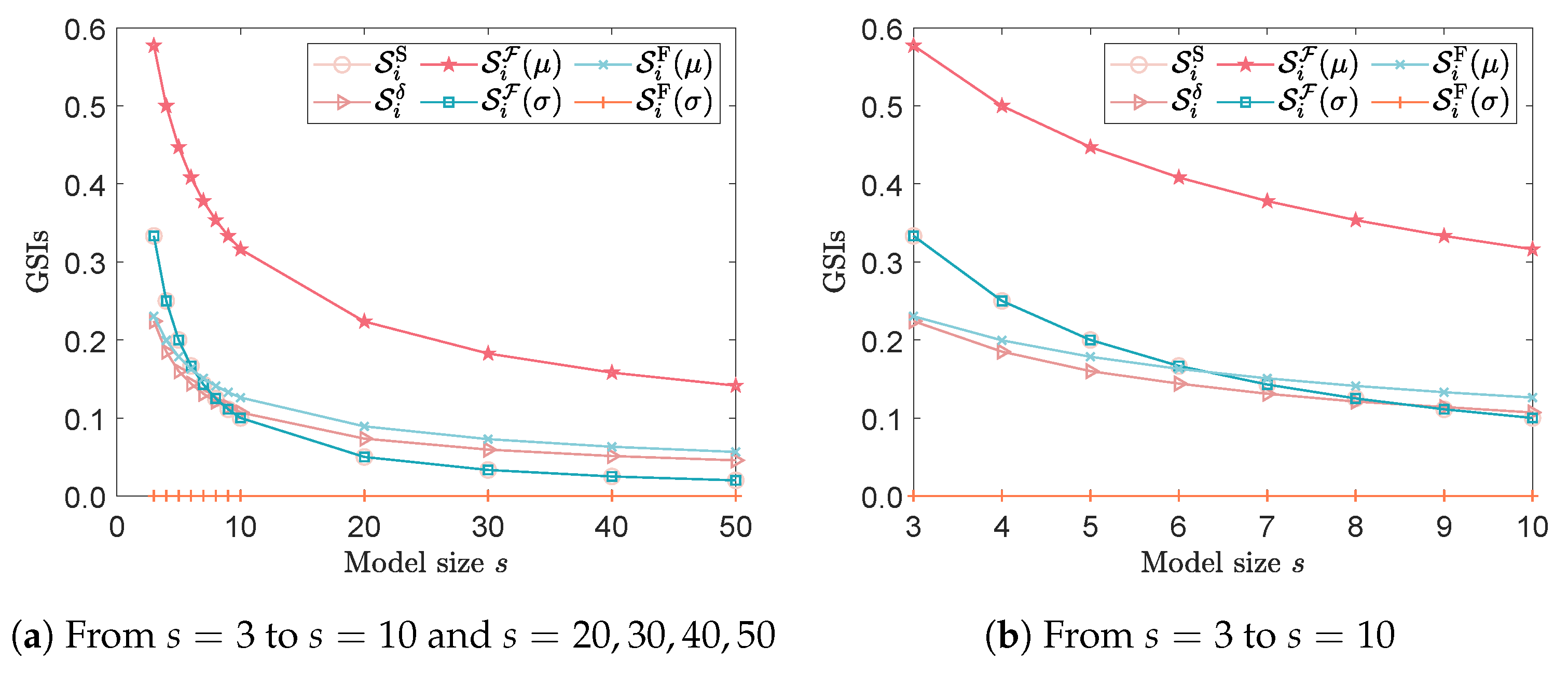
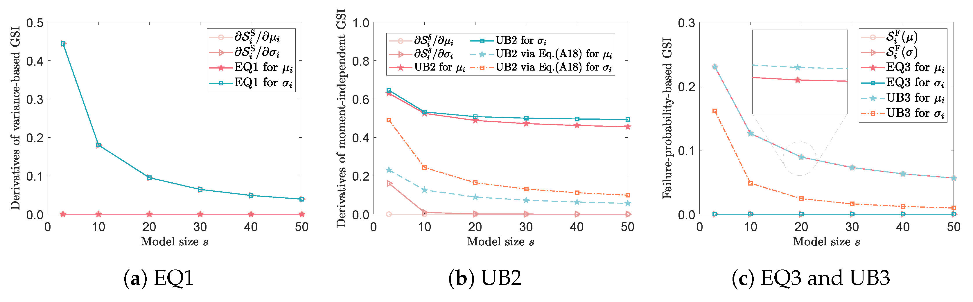
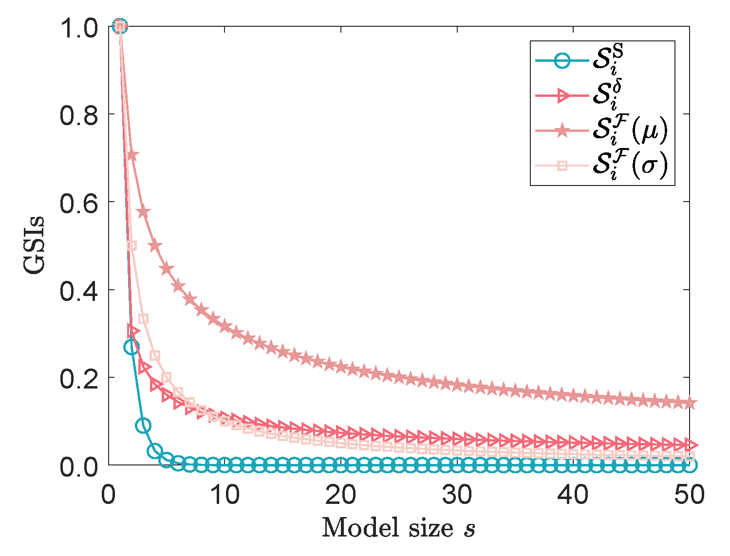
5.3. Example 3: Borgonovo’s Growing Size Model

Consider Borgonovo’s growing size model [16] as follows:

$$X=\sum _{i=1}^s{\mathrm{\Theta }}_i,$$

(39)

where the ${\mathrm{\Theta }}_i$’s are i.i.d. normal random variables with mean value ${\mu }_i$ and standard deviation ${\sigma }_i$, and s stands for the size of the model. Obviously, X follows the normal distribution with mean value ${\mu }_X={\sum }_{i=1}^s{\mu }_i$ and variance ${\sigma }_X^2={\sum }_{i=1}^s{\sigma }_i^2$. The derivatives of PDF of X with respect to ${\mu }_i$ and ${\sigma }_i$ for $i=1,2,\cdots ,s$ can be read as follows:

$$\left\{\begin{array}{cc}\hfill {\displaystyle \frac{\partial p_X}{\partial {\mu }_i}}& ={\displaystyle \frac{x-{\mu }_X}{{\sigma }_X^2}}{p}_X(x;{\mu }_X,{\sigma }_X),\hfill \\ \hfill {\displaystyle \frac{\partial p_X}{\partial {\sigma }_i}}& ={\displaystyle \frac{{(x-{\mu }_X)}^2-{\sigma }_X^2}{{\sigma }_X^3}}{\displaystyle \frac{{\sigma }_i}{{\sigma }_X}}{p}_X(x;{\mu }_X,{\sigma }_X).\hfill \end{array}\right.$$

(40)

Note that for the normal distribution with mean value ${\mu }_i$ and standard deviation ${\sigma }_i$ there are [10]

$$\left\{\begin{array}{cc}\hfill ∥{\displaystyle \frac{\partial p_{{\mathrm{\Theta }}_i}({\theta }_i;{\mu }_i,{\sigma }_i)}{\partial {\mu }_i}}∥& ={\displaystyle \frac{1}{\sqrt{2\pi }{\sigma }_i}},\hfill \\ \hfill ∥{\displaystyle \frac{\partial p_{{\mathrm{\Theta }}_i}({\theta }_i;{\mu }_i,{\sigma }_i)}{\partial {\sigma }_i}}∥& ={\displaystyle \frac{2}{\sqrt{2\pi }{\sigma }_i}}{e}^{-1/2}.\hfill \end{array}\right.$$

(41)

Then, the analytical IMs from the Fre-GSIs in terms of ${\mu }_i$ and ${\sigma }_i$ are ${\sigma }_i/{\sigma }_X$ and ${\sigma }_i^2/{\sigma }_X^2$, respectively.

Let ${\mu }_i=0$ and ${\sigma }_i=1$ for $i=1,2,\cdots ,s$. Obviously, the variance-based GSI for ${\mathrm{\Theta }}_i$ is $1/s$. The conditional PDF $X|{\mathrm{\Theta }}_i$ admits $\mathcal{N}({\mathrm{\Theta }}_i,\sqrt{s-1})$; therefore, the moment-independent GSI can be numerically computed by

$$S_i^{\delta }={\displaystyle \frac{1}{2}}{\mathbb{E}}_{{\mathrm{\Theta }}_i}\left[{\int }_{{\mathrm{\Omega }}_X}\left|\mathcal{N}(0,\sqrt{s})-\mathcal{N}({\mathrm{\Theta }}_i,\sqrt{s-1})\right|\mathrm{d}x\right],$$

(42)

and the IMs computed from the Fre-GSIs in terms of ${\mu }_i$ and ${\sigma }_i$ are $1/\sqrt{s}$ and $1/s$, respectively. The failure-probability-based GSIs can be obtained by integrating Equation (40) in the failure domain, whose formulas are omitted for the sake of brevity.

Let the model size s grow from 3 to 50. The values of the four GSIs with increasing s are summarized in Figure 8. Since the failure-probability-based GSI is dependent on the failure domain, we set ${\mathrm{\Omega }}_{\mathrm{F}}:x>0$, which ensures that the same failure probability equals $0.5$ as the model size increases. The four GSIs decrease expectedly as s increases, which is in accordance with our intuition [16]: one out of 3 summed i.i.d. inputs plays a more important role than one out of 50 summed i.i.d. inputs on one’s degree of belief. This result can also be observed in Figure 9, where the amplitude of Fre-GSI decreases as the model size increases. The analytical values of $\partial S_i^{\mathrm{S}}/\partial {\mu }_i$ and $\partial S_i^{\mathrm{S}}/\partial {\sigma }_i$ are 0 and $2(s-1)/s^2$, respectively, while $\partial S_i^{\delta }/\partial {\mu }_i$ and $\partial S_i^{\delta }/\partial {\sigma }_i$ are calculated with the central difference scheme using the difference size of $0.1$. Again, the proposed links of the Fre-GSI with the other GSIs are verified in Figure 10. Additionally, a lower UB2 can be obtained by Equation (A17) in Appendix A.4 if the total variation distance between the conditional and unconditional PDFs of X is available. Otherwise, the proposed UB2 in Equation (31) may be a good alternative.

Moreover, in Figure 8, one can see that $S_i^{\mathrm{S}}$ decreases faster than $S_i^{\delta }$, $S_i^{\mathcal{F}}\left(\mu \right)$ and $S_i^{\mathrm{F}}\left(\mu \right)$. Note that $S_i^{\mathcal{F}}\left(\mu \right)$ has the largest value among the GSIs, while $S_i^{\mathrm{F}}\left(\sigma \right)$ is zero, thus cannot provide informative results for global sensitivity analysis. Another feature of the variance-based GSI can be observed when considering Borgonovo’s growing size model with a multiplicative structure [16], i.e.,

$$X=\prod _{i=1}^s{\mathrm{\Theta }}_i,$$

(43)

where ${\mathrm{\Theta }}_i$ is independently distributed with the lognormal distribution $\mathcal{LN}({\theta }_i;{\mu }_i,{\sigma }_i)$, in which ${\mu }_i$ and ${\sigma }_i$ are the mean value and standard deviation of $ln{\mathrm{\Theta }}_i$, respectively.

Denote ${\mu }_i=0$ and ${\sigma }_i=1$ for $i=1,2,\cdots ,s$. In this case, $S_i^{\delta }$, $S_i^{\mathcal{F}}\left(\mu \right)$ and $S_i^{\mathcal{F}}\left(\sigma \right)$ remain the same as the case in Equation (39), while $S_i^{\mathrm{S}}$ changes to [16]

$$S_i^{\mathrm{S}}=1-{\displaystyle \frac{e^s-e}{e-1}},$$

(44)

where s ranges from 1 to 50. In Figure 11, it is seen that $S_i^{\mathrm{S}}$ decreases rapidly as the model size grows. Further, we extend Borgonovo’s interpretation [16] to explain why the moment-independent GSI, and especially the Fre-GSI, can deliver more information on the sensitivity analysis than the variance-based GSI. Considering the case $s=5$ that $S_i^{\mathrm{S}}=0.012$, $S_i^{\delta }=0.160$, $S_i^{\mathcal{F}}\left(\mu \right)=0.447$ and $S_i^{\mathcal{F}}\left(\sigma \right)=0.200$. If the standard deviation of ${\mathrm{\Theta }}_i$ is reduced by around $0.01$, then, based on $S_i^{\mathrm{S}}$ the decision-maker, we may conclude that knowing ${\mathrm{\Theta }}_i$ with certainty would not have a remarkable effect on its uncertainty. Instead, both $S_i^{\delta }$ and $S_i^{\mathcal{F}}\left(\sigma \right)$ show that fixing one out of the five inputs will result in a non-negligible shift in the PDF of X. In addition, $S_i^{\mathcal{F}}\left(\mu \right)$ implies that the PDF of X is more sensitive to the mean value than to the standard deviation. Nevertheless, the variance-based GSI and the moment-independent GSI would not deliver this information.

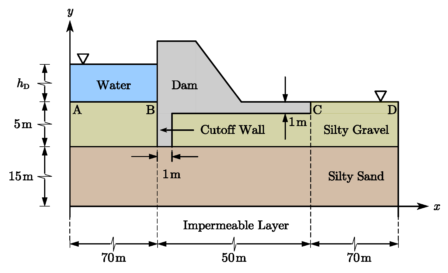
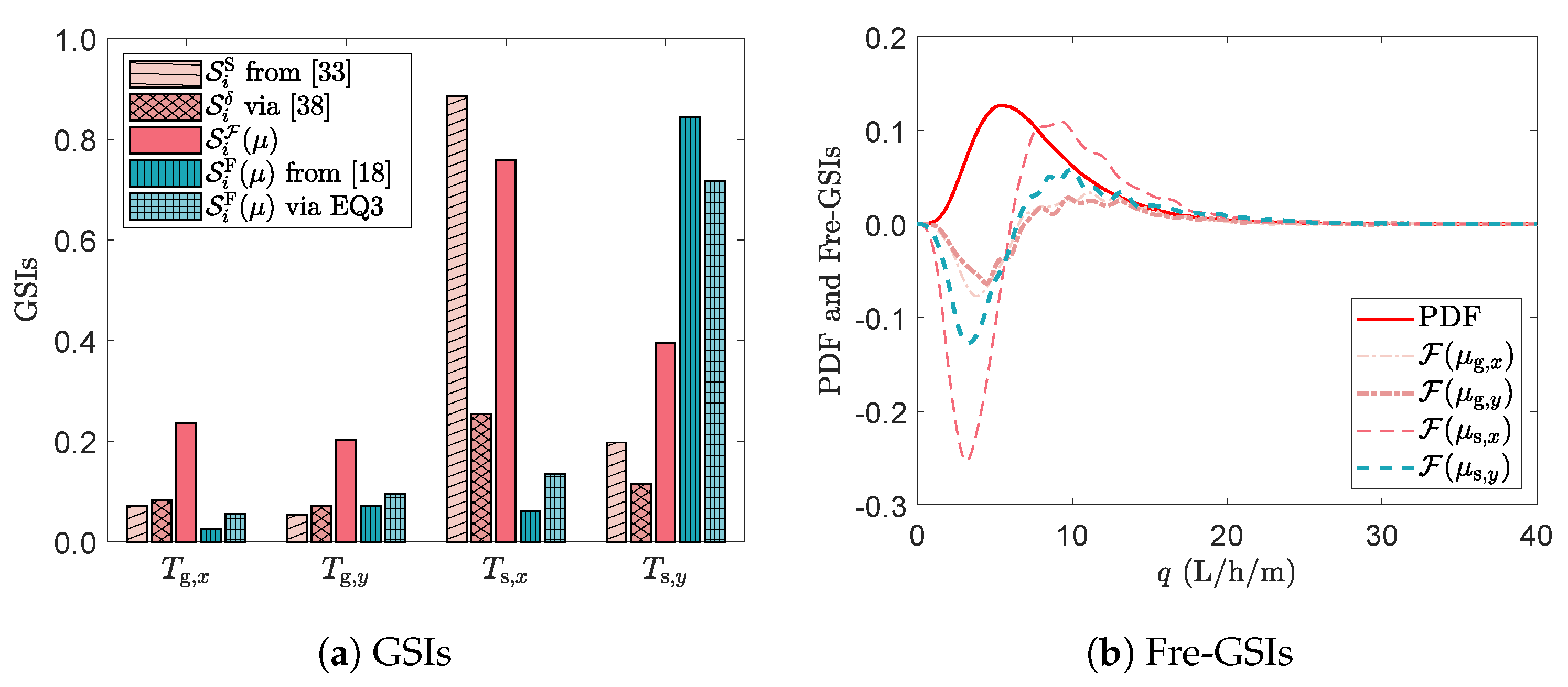
5.4. Example 4: A Dam Seepage Model

The last example involves the sensitivity analysis of a steady-state confined seepage below a dam [18], as shown in Figure 12. During the analysis, it is assumed that the seepage is anisotropic and uniform. The permeability parameters of the silty gravel layer are denoted as $T_{\mathrm{g},x}$ (in x-direction) and $T_{\mathrm{g},y}$ (in y-direction), while those of the silty sand layers are defined by $T_{\mathrm{s},x}$ (in x-direction) and $T_{\mathrm{s},y}$ (in y-direction).

The governing equation of the seepage problem in Figure 12 reads as follows:

$$\left\{\begin{array}{c}\hfill T_{\mathrm{g},x}{\displaystyle \frac{{\partial }^2{h}_{\mathrm{W}}}{\partial x^2}}+T_{\mathrm{g},y}{\displaystyle \frac{{\partial }^2{h}_{\mathrm{W}}}{\partial y^2}}=0,\\ \hfill T_{\mathrm{s},x}{\displaystyle \frac{{\partial }^2{h}_{\mathrm{W}}}{\partial x^2}}+T_{\mathrm{s},y}{\displaystyle \frac{{\partial }^2{h}_{\mathrm{W}}}{\partial y^2}}=0,\end{array}\right.$$

(45)

and the seepage discharge q at the downstream side of the dam is calculated by

$$q=-{\int }_{{\mathrm{\Omega }}_{\mathrm{CD}}}{T}_{\mathrm{g},y}{\displaystyle \frac{\partial h_{\mathrm{W}}(x,y)}{\partial y}}\mathrm{d}x,$$

(46)

where the hydraulic head $h_{\mathrm{W}}$ on the AB segment is equal to $20+h_{\mathrm{D}}$, and the failure event is defined when the seepage discharge q exceeds the threshold $q_{\lim }=30$ (L/h/m). In the dam seepage model, the five input parameters $\left\{T_{\mathrm{g},x},T_{\mathrm{g},y},T_{\mathrm{s},x},T_{\mathrm{s},y},h_{\mathrm{D}}\right\}$ are considered independent random variables, where their probabilistic information is listed in

Table 2. Uncertain parameters in the dam seepage model (Example 4).

Parameters	Distribution	(Mean, SD)
$T_{\mathrm{g},x}$	Lognormal	$(5\times {10}^{-6}, 5\times {10}^{-6})$ (m/s)
$T_{\mathrm{g},y}$	Lognormal	$(2\times {10}^{-6}, 2\times {10}^{-6})$ (m/s)
$T_{\mathrm{s},x}$	Lognormal	$(5\times {10}^{-7}, 5\times {10}^{-7})$ (m/s)
$T_{\mathrm{s},y}$	Lognormal	$(2\times {10}^{-7}, 2\times {10}^{-7})$ (m/s)
$h_{\mathrm{D}}$	Uniform	$(8.5,\sqrt{3}/2)$ (m)

. The deterministic analysis of Equation (45) is conducted by the finite element method with a total of 3413 nodes and 1628 quadratic triangular elements.

Different GSIs of the first four parameters in Table 2 are calculated for the sensitivity analysis, including the variance-based GSI $S_i^{\mathrm{S}}$, the moment-independent GSI $S_i^{\delta }$, the importance measures $S_i^{\mathcal{F}}\left(\mu \right)$ based on the Fre-GSI (with respect to the mean value), and the failure-probability-based GSI $S_i^{\mathrm{F}}\left(\mu \right)$ (with respect to the mean value). The GSA results are presented in Figure 13, where $S_i^{\mathrm{S}}$ and $S_i^{\mathrm{F}}\left(\mu \right)$ are adopted from [18], respectively; $S_i^{\delta }$ is calculated by using ${10}^6$ MCS samples, while $S_i^{\mathcal{F}}\left(\mu \right)$ is computed via the central difference method [10] by taking $10\%$ of the mean value as the difference size. Note that the absolute value of $S_i^{\mathrm{F}}\left(\mu \right)$ is much higher than 1, since the mean value of the permeability parameter is very small. Hence, to facilitate discussion, all the results of $S_i^{\mathrm{F}}\left(\mu \right)$ shown in Figure 13a are after normalization, i.e., $S_i^{\mathrm{F}}\left(\mu \right)\to S_i^{\mathrm{F}}\left(\mu \right)/{\sum }_{i=1}^4{S}_i^{\mathrm{F}}\left(\mu \right)$.

From Figure 13a, it can be seen that the results of $S_i^{\mathrm{F}}\left(\mu \right)$ via EQ3 are very close to the ones from [18]. The results of $S_i^{\mathrm{F}}\left(\mu \right)$ indicate that the permeability of the silty sand layer in the y-direction, i.e., $T_{\mathrm{s},y}$ has the largest impact on the seepage discharge q, while the influence of $T_{\mathrm{g},x}$ can be ignored. However, according to the results of $S_i^{\mathrm{S}}$, $S_i^{\delta }$ and $S_i^{\mathcal{F}}\left(\mu \right)$, the permeability of the silty sand layer in the x-direction, i.e., $T_{\mathrm{s},x}$ accounts for the top contribution to the uncertainty of the seepage discharge, which can also be seen clearly from the Fre-GSIs shown in Figure 13b. The above results further substantiate the notion previously articulated that the implementation of a singular GSI for the GSA may yield relatively one-sided quantification outcomes.

6. Conclusions

In this work, three classical global sensitivity indices (GSIs), i.e., variance-based GSI, moment-independent GSI, and failure-probability-based GSI, are revisited, and some properties of a newly developed Fréchet-derivative-based GSI (Fre-GSI) are studied. A functional perspective of the stochastic parametric model of complex systems is proposed for revealing the physical meanings of the four GSIs in a unified description. Some practical links of the Fre-GSI with the other three GSIs are derived. Test examples are studied to verify the proposed links, and specific performances of the four GSIs are investigated as well. The main findings and conclusions are as follows:

• The importance measure and direction indicator are obtained from the Fre-GSI, whose basic properties are studied to illustrate the ability of Fre-GSI for global sensitivity analysis.
• The four GSIs can be clearly comprehended through a functional description, wherein the distinctions among the four GSIs stem from the definitions of stochastic distances computed by different operators.
• Some practical links of the Fre-GSI with other GSIs are analytically derived and verified numerically.
• The complementary nature of the four GSIs is revealed. The variance-based GSI can effectively reflect the model structure, while the moment-independent GSI can reflect the uncertainty in distribution. The failure-probability-based GSI is useful for quantifying the impact of different failure criteria, while the Fre-GSI has robust capabilities on the importance measure and the direction of sensitivity.

It is noteworthy to mention that while the selected examples are of a simplistic nature, they can serve as effective benchmarks for readers seeking a concise comprehension of the basic features of the four GSIs. Open issues remain to be studied in the future, e.g., the stronger connections between the Fre-GSI and the other GSIs (but not limited to the three types studied), especially for complex engineering structures involving high-dimensional and/or dependent inputs, as well as multivariate and/or time-dependent outputs.

References

1. Ehre, M.; Papaioannou, I.; Straub, D. Global sensitivity analysis in high dimensions with PLS-PCE. Reliab. Eng. Syst. Saf. 2020, 198, 106861. [Google Scholar] [CrossRef]
2. Papaioannou, I.; Straub, D. Variance-based reliability sensitivity analysis and the FORM α-factors. Reliab. Eng. Syst. Saf. 2021, 210, 107496. [Google Scholar] [CrossRef]
3. Wan, Z.Q.; Tao, W.F.; Ding, Y.Q.; Xin, L.F. Fréchet-derivative-based global sensitivity analysis of the physical random function model of ground motions. Dis. Prev. Res. 2023, 2, 8. [Google Scholar] [CrossRef]
4. Hong, X.; Wan, Z.Q.; Chen, J.B. Parallel assessment of the tropical cyclone wind hazard at multiple locations using the probability density evolution method integrated with the change of probability measure. Reliab. Eng. Syst. Saf. 2023, 237, 109351. [Google Scholar] [CrossRef]
5. Jung, W.H.; Taflanidis, A.A. Efficient global sensitivity analysis for high-dimensional outputs combining data-driven probability models and dimensionality reduction. Reliab. Eng. Syst. Saf. 2023, 231, 108805. [Google Scholar] [CrossRef]
6. Shang, Y.; Nogal, M.; Teixeira, R.; Wolfert, A. Extreme-oriented sensitivity analysis using sparse polynomial chaos expansion. Application to train–track–bridge systems. Reliab. Eng. Syst. Saf. 2024, 243, 109818. [Google Scholar] [CrossRef]
7. Derennes, P.; Morio, J.; Simatos, F. Simultaneous estimation of complementary moment independent and reliability-oriented sensitivity measures. Math. Comput. Simulat. 2021, 182, 721–737. [Google Scholar] [CrossRef]
8. Ma, Y.Z.; Jin, X.X.; Zhao, X.; Li, H.S.; Zhao, Z.Z.; Xu, C. Reliability-oriented global sensitivity analysis using subset simulation and space partition. Reliab. Eng. Syst. Saf. 2024, 242, 109794. [Google Scholar] [CrossRef]
9. Torii, A.J.; Novotny, A.A. A priori error estimates for local reliability-based sensitivity analysis with Monte Carlo Simulation. Reliab. Eng. Syst. Saf. 2021, 213, 107749. [Google Scholar] [CrossRef]
10. Chen, J.B.; Wan, Z.Q.; Beer, M. A global sensitivity index based on Fréchet derivative and its efficient numerical analysis. Probabilistic Eng. Mech. 2020, 62, 103096. [Google Scholar] [CrossRef]
11. Chen, J.B.; Yang, J.S.; Jensen, H. Structural optimization considering dynamic reliability constraints via probability density evolution method and change of probability measure. Struct. Multidiscip. Optim. 2020, 62, 2499–2516. [Google Scholar] [CrossRef]
12. Saltelli, A.; Tarantola, S.; Campolongo, F.; Ratto, M. Sensitivity Analysis in Practice: A Guide to Assessing Scientific Models; John Wiley & Sons: Chichester, UK, 2004. [Google Scholar]
13. Sobol’, I.M. Sensitivity estimates for nonlinear mathematical models. Math. Model. Comput. Exp. 1993, 1, 407–414. [Google Scholar]
14. Mara, T.A.; Tarantola, S. Variance-based sensitivity indices for models with dependent inputs. Reliab. Eng. Syst. Saf. 2012, 107, 115–121. [Google Scholar] [CrossRef]
15. Borgonovo, E. A new uncertainty importance measure. Reliab. Eng. Syst. Saf. 2007, 92, 771–784. [Google Scholar] [CrossRef]
16. Borgonovo, E.; Castaings, W.; Tarantola, S. Moment independent importance measures: New results and analytical test cases. Risk Anal. 2011, 31, 404–428. [Google Scholar] [CrossRef]
17. Wu, Y.T. Computational methods for efficient structural reliability and reliability sensitivity analysis. AIAA J. 1994, 32, 1717–1723. [Google Scholar] [CrossRef]
18. Valdebenito, M.A.; Jensen, H.; Hernández, H.B.; Mehrez, L. Sensitivity estimation of failure probability applying line sampling. Reliab. Eng. Syst. Saf. 2018, 171, 99–111. [Google Scholar] [CrossRef]
19. Perrin, G.; Defaux, G. Efficient evaluation of reliability-oriented sensitivity indices. J. Sci. Comput. 2019, 79, 1433–1455. [Google Scholar] [CrossRef]
20. Lemaître, P.; Sergienko, E.; Arnaud, A.; Bousquet, N.; Gamboa, F.; Iooss, B. Density modification-based reliability sensitivity analysis. J. Stat. Comput. Simul. 2015, 85, 1200–1223. [Google Scholar] [CrossRef]
21. Helton, J.C.; Johnson, J.D.; Sallaberry, C.J.; Storlie, C.B. Survey of sampling-based methods for uncertainty and sensitivity analysis. Reliab. Eng. Syst. Saf. 2006, 91, 1175–1209. [Google Scholar] [CrossRef]
22. Ghanem, R.; Higdon, D.; Owhadi, H. (Eds.) Handbook of Uncertainty Quantification; Springer International Publishing: Cham, Switzerland, 2017. [Google Scholar]
23. Borgonovo, E. Measuring uncertainty importance: Investigation and comparison of alternative approaches. Risk Anal. 2006, 26, 1349–1361. [Google Scholar] [CrossRef] [PubMed]
24. Iooss, B.; Le Gratiet, L. Uncertainty and sensitivity analysis of functional risk curves based on Gaussian processes. Reliab. Eng. Syst. Saf. 2019, 187, 58–66. [Google Scholar] [CrossRef]
25. Lamboni, M.; Kucherenko, S. Multivariate sensitivity analysis and derivative-based global sensitivity measures with dependent variables. Reliab. Eng. Syst. Saf. 2021, 212, 107519. [Google Scholar] [CrossRef]
26. Vuillod, B.; Montemurro, M.; Panettieri, E.; Hallo, L. A comparison between Sobol’s indices and Shapley’s effect for global sensitivity analysis of systems with independent input variables. Reliab. Eng. Syst. Saf. 2023, 234, 109177. [Google Scholar] [CrossRef]
27. Li, J.; Chen, J.B. The principle of preservation of probability and the generalized density evolution equation. Struct. Saf. 2008, 30, 65–77. [Google Scholar] [CrossRef]
28. Grigoriu, M. Stochastic Systems: Uncertainty Quantification and Propagation; Springer: London, UK, 2012. [Google Scholar]
29. Wan, Z.Q.; Chen, J.B.; Beer, M. Functional perspective of uncertainty quantification for stochastic parametric systems and global sensitivity analysis. Chin. J. Theor. Appl. Mech. 2021, 53, 837–854. [Google Scholar]
30. Rubinstein, R.Y. Sensitivity analysis and performance extrapolation for computer simulation models. Oper. Res. 1989, 37, 72–81. [Google Scholar] [CrossRef]
31. Homma, T.; Saltelli, A. Importance measures in global sensitivity analysis of model output. Reliab. Eng. Syst. Saf. 1996, 52, 1–17. [Google Scholar] [CrossRef]
32. Da Veiga, S.; Gamboa, F.; Iooss, B.; Prieur, C. Basics and Trends in Sensitivity Analysis; Society for Industrial and Applied Mathematics: Philadelphia, PA, USA, 2021. [Google Scholar]
33. Liu, Q.; Homma, T. A new importance measure for sensitivity analysis. J. Nucl. Sci. 2010, 47, 53–61. [Google Scholar] [CrossRef]
34. Wan, Z.Q.; Chen, J.B.; Li, J.; Ang, A.H.-S. An efficient new PDEM-COM based approach for time-variant reliability assessment of structures with monotonically deteriorating materials. Struct. Saf. 2020, 82, 101878. [Google Scholar] [CrossRef]
35. Borgonovo, E.; Plischke, E. Sensitivity analysis: A review of recent advances. Eur. J. Oper. Res. 2016, 248, 869–887. [Google Scholar] [CrossRef]
36. Torii, A.J. On sampling-based schemes for probability of failure sensitivity analysis. Probabilistic Eng. Mech. 2020, 62, 103099. [Google Scholar] [CrossRef]
37. Chen, J.B.; Wan, Z.Q. A compatible probabilistic framework for quantification of simultaneous aleatory and epistemic uncertainty of basic parameters of structures by synthesizing the change of measure and change of random variables. Struct. Saf. 2019, 78, 76–87. [Google Scholar] [CrossRef]
38. Zhao, Y.G.; Zhang, X.Y.; Lu, Z.H. A flexible distribution and its application in reliability engineering. Reliab. Eng. Syst. Saf. 2018, 176, 1–12. [Google Scholar] [CrossRef]
39. Li, J.; Chen, J.B. Stochastic Dynamics of Structures; John Wiley & Sons: Singapore, 2009. [Google Scholar]
40. Wan, Z.Q. Global sensitivity evolution equation of the Fréchet-derivative-based global sensitivity analysis. Struct. Saf. 2024, 106, 102413. [Google Scholar] [CrossRef]
41. Wainwright, H.M.; Finsterle, S.; Jung, Y.; Zhou, Q.L.; Birkholzer, J.T. Making sense of global sensitivity analyses. Comput. Geosci. 2014, 65, 84–94. [Google Scholar] [CrossRef]
42. Atkinson, K.; Han, W.M. Theoretical Numerical Analysis: A Functional Analysis Framework; Springer Science & Business Media: New York, NY, USA, 2009. [Google Scholar]
Figure 1. Illustration of the three classical GSIs.
Applsci 15 02703 g001
Figure 2. The functional perspective on the stochastic model and the Fréchet-derivative-based GSI.
Applsci 15 02703 g002
Figure 3. Illustration of the Fre-GSI and the corresponding direction indicator.
Applsci 15 02703 g003
Figure 4. A functional perspective to illustrate the essences of four classes of GSIs.
Applsci 15 02703 g004aApplsci 15 02703 g004b
Figure 5. Fre-GSIs of Equations (10) and (34) (Example 1).
Applsci 15 02703 g005
Figure 6. Analytical PDF of X and its corresponding Fre-GSIs (Example 2).
Applsci 15 02703 g006
Figure 7. F ( μ 2 ) with fixed μ 1 = 0 , σ 1 = σ 2 = 1 , and μ 2 [ 2 , 2 ] (Example 2).
Applsci 15 02703 g007
Figure 8. The four GSIs with increasing model size (Example 3).
Applsci 15 02703 g008
Figure 9. Fre-GSIs with growing model size s (Example 3).
Applsci 15 02703 g009
Figure 10. Verification of EQ1, UB2, EQ3, and UB3 (Example 3).
Applsci 15 02703 g010
Figure 11. GSIs for Borgonovo’s growing size model with a multiplicative structure (Example 3).
Applsci 15 02703 g011
Figure 12. Schematic representation of the dam seepage model (Example 4).
Applsci 15 02703 g012
Figure 13. Results of GSA (Example 4).
Applsci 15 02703 g013