Abstract
To address the challenge of simulating force–thermal environmental loads on morphing wings during flight, this study proposes and validates a force–thermal simulation method based on servo loading. First, the aerodynamic loads on a multi-stage telescopic wing under extreme conditions were systematically analyzed to identify the critical design loads. Subsequently, a force–thermal servo loading platform for multi-stage telescopic wings was designed and constructed to evaluate the performance of the wing’s morphing mechanism during flight. A dynamic multi-point equivalent method based on grid reconstruction was proposed and theoretically derived, along with simulations using a traditional multi-point load distribution method. Compared to the conventional equal-area division method, the simulation results demonstrated a significant improvement in deformation fitting accuracy using the proposed method. Finally, force–thermal servo loading experiments were conducted on a prototype of the multi-stage telescopic wing. The results verified that the proposed loading method can accurately simulate load variations during flight, with experimental trends closely aligning with simulation predictions. Additionally, the experiments demonstrated the loading system’s rapid response capability, confirming the feasibility and potential of the designed loading platform and theoretical model. This research provides critical technical support and theoretical foundations for the design, validation, and force–thermal environment simulation of future multidimensional morphing wings.
1. Introduction
As the complexity of aircraft applications in the aerospace field continues to grow, modern aircraft are required to operate across broader flight envelopes and speed ranges. Traditional fixed-geometry aircraft are unable to adapt to such variable flight environments and mission requirements, thereby limiting their performance under specific conditions [1,2]. In contrast, morphing aircraft can adjust their configurations based on mission demands, environmental conditions, and their own operational states, allowing them to adapt to diverse flight scenarios. To date, various morphing aircraft have entered service and demonstrated excellent adaptability [3,4,5,6,7]. Morphing wings are a critical research area within the broader domain of morphing aircraft. After their design is completed, these wings must undergo a series of tests to validate their performance, especially in terms of failure modes, operational reliability, and safety under different flight conditions. Unlike traditional fixed-wing loading methods, morphing wings can change their aerodynamic shape, necessitating continuous loading during ground testing to match their deformation process. Therefore, the loading system must provide servo-controlled loading synchronized with the wing’s deformation to ensure the accuracy of the test results [8,9,10].
Currently, research on servo-controlled loading devices for morphing wings remains limited. Zheng et al. designed an experimental setup for folding wing deployment, simulating lift loading during the deployment process using cylinders and bearing components. Their study found that lift had a significant impact on the deployment time of folding wings [11,12]. Beyond this, most related studies focus on servo-controlled loading devices for slat and flap morphing. For instance, Pang et al. analyzed the advantages and disadvantages of three servo-loading techniques, namely synthetic loading, pivot loading, and multi-degree-of-freedom separated loading, recommending methods based on specific objectives [13]. Zhang et al. proposed a dual-actuator servo-controlled loading technique with sliding carriages, addressing the challenge of changing normal load directions during the deflection of movable wing surfaces [14]. Li et al. utilized finite element analysis to divide wing deformation into multiple flight points, employing a dual-actuator servo system to maintain a high degree of perpendicularity between the loading force and wing surface during large deformations [15]. Du Feng et al. designed a separated servo-controlled loading device that was successfully applied in flap fatigue testing, achieving precise control of the load magnitude and direction [16]. However, most existing studies have targeted simpler deformation mechanisms with limited ranges, such as those in slats and flaps. In contrast, morphing wings exhibit large and complex deformations, making traditional static test methods inadequate for accurately simulating their actual deformation processes.
To better simulate aerodynamic loading, Sun highlighted common methods for transferring aerodynamic grid loads to finite element structural grids, including three-point, four-point, and multi-point methods [17]. Wang [18] provided a detailed implementation process for the multi-point method and applied it to the aerodynamic load distribution of an aircraft’s horizontal tail. Lei Li et al. [19] compared the three-point, four-point, and multi-point methods through case studies, concluding that these approaches effectively transfer aerodynamic grid loads to structural grids. When structural grid nodes coincide with predefined loading points, aerodynamic grid loads can be equivalently transferred to these points. While these methods work well for fixed-wing load equivalency, they are not suitable for morphing wings, where surface areas change dynamically during deformation.
In terms of thermal load simulation, research both domestically and internationally focuses on two primary approaches: convective and non-convective methods [20]. Jia et al. introduced a method for simulating the thermal environment of a hypersonic vehicle nose cone using high-temperature gas injection [21]. Wu et al. conducted thermal–vibration coupling experiments on lightweight thermal protection materials under conditions up to 1500 °C [22]. Tan et al. developed a thermal modal testing device for aircraft wing structures, performing a variety of heating experiments [23].
In summary, the dynamic loading conditions experienced by wings during flight are highly variable, and traditional static tests cannot fully represent the complex and variable coupled force–thermal loads encountered in real flight scenarios. Thus, conducting experimental research on servo-controlled force–thermal loading for the entire motion process of multi-stage telescopic wings is of significant importance for realistically simulating the environmental loads experienced during service.
This study focuses on a multi-stage telescopic wing designed for this purpose. The aerodynamic loads, particularly under extreme conditions, are analyzed to determine the design benchmark loads. A force–thermal servo-controlled loading platform is then developed to verify the performance of the wing’s deformation mechanism during flight. By integrating the multi-point load distribution method with grid reconstruction, a dynamic multi-point equivalency method is proposed to transfer aerodynamic loads to predefined loading points. Its feasibility and advantages are validated through comparison with the traditional equal-area distribution method. Finally, servo-controlled force–thermal loading experiments are conducted on the prototype of the multi-stage telescopic wing, verifying the capability of the proposed method to accurately simulate the load variation experienced by the wing during flight.
2. Aerodynamic Load and Deformation Analysis of Multi-Stage Telescopic Wings
As shown in Figure 1, to enable the aircraft to perform diverse flight profiles, such as long-duration cruising and high-speed penetration, while minimizing the occupation of internal space, this study proposes a high space-utilization multi-stage telescopic wing design. This design allows the telescopic wing to adapt to various flight mission profiles with almost no impact on the internal space of the aircraft. The lift-to-drag ratio of the telescopic wing changes by between 20% and 70% between the fully retracted and fully extended states. Consequently, the aerodynamic shape can be adjusted to suit different flight environments across varying speed regimes, significantly enhancing the wide-speed-range service performance of the aircraft.
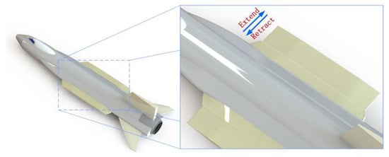
Figure 1.
Telescoping wing aircraft.
The geometric model of the multi-stage telescopic wing is shown in Figure 2. Figure 2a illustrates the motion mechanism, where the multi-stage telescopic wing adopts a lap joint configuration. In practical applications, the wing root is fixed to the aircraft structure to provide stable support, while the other end of the telescopic wing remains free. The first-stage and second-stage telescopic wings achieve rapid, synchronized, and repeatable extension and retraction under the actuation of a dual-screw–nut mechanism. This mechanism features a self-locking capability, allowing the telescopic wing to stop at any position, thereby enabling multiple configurations. The guide rail and slider provide directional constraints for the telescopic motion, while the second-stage wing extension is synchronized through a motor-driven screw mechanism.
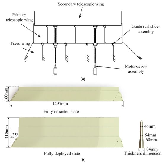
Figure 2.
Telescoping wing aircraft. (a) Schematic diagram of mechanism composition; (b) dimensional parameter model.
Figure 2b presents the key dimensional parameters of the multi-stage telescopic wing. The airfoil used in this study is a non-standard airfoil, defined through a 3D CAD model. The root chord length of the telescopic wing is 1495 mm, with a fixed-section wingspan of 150 mm, a first-stage telescopic wingspan of 140 mm, and a second-stage telescopic wingspan of 136 mm. The wall thickness of each wing section is 1.5 mm, while the wall thickness at the reinforced rib sections is designed to be 4 mm. The wing has a fixed sweep angle of 35° and a thickness-to-chord ratio of 5.62%. Additionally, the tip-to-root chord length ratio is 0.86. The total wingspan of the wing in its fully extended state is 410 mm, whereas in the fully retracted state, it is 160 mm.
The aerodynamic forces, aerodynamic heating, vibrations, and noise loads encountered in a hypersonic flight environment are extremely severe. Consequently, the load-bearing and transmission structures of the multi-stage telescopic wing impose stringent requirements on the comprehensive performance of materials under high-temperature conditions. High-temperature alloys exhibit superior strength at elevated temperatures, among which GH4169 demonstrates excellent oxidation resistance, fatigue resistance, and corrosion resistance over a wide temperature range of −253 °C to 700 °C. Notably, at temperatures not exceeding 650 °C, GH4169 possesses the highest strength among high-temperature alloys. Additionally, GH4169 offers excellent machinability, weldability, and long-term stability, enabling the fabrication of complex structural components. Therefore, GH4169 is selected as the primary material for the wing structure. The material has a density of 8240 kg/m3, and its mechanical properties, including elastic modulus and thermal expansion coefficient, vary with temperature. Detailed material properties are presented in Table 1.

Table 1.
Physical and thermal properties of GH4169.
2.1. Aerodynamic Analysis of Flight Environmental Loads
In the design and validation of a multi-stage telescopic wing, the aerodynamic load analysis under flight conditions is a critical step for evaluating wing performance and ensuring structural reliability. This section conducts a simulation analysis of force–thermal loads experienced by the telescopic wing in the flight environment.
2.1.1. Flow Field Model Establishment
The intended operational environment for the multi-stage telescopic wing corresponds to a maximum flight speed of Ma = 5 and a maximum flight altitude of 20 km. The aerodynamic analysis is conducted based on its maximum flight capability as the design condition. First, the standard atmospheric parameters under the specified design condition are determined, as listed in Table 2.
Table 2.
Atmospheric parameters under design conditions.
For flow field modeling, a rectangular computational domain is selected to minimize the influence of fluid domain inlets and outlets on the results and ensure an adequate fluid region around the telescopic wing. The telescopic wing is positioned at the center of the domain, with the front designated as the inflow inlet and the rear as the outflow outlet. The other four sides are set as flow field boundaries to avoid undesired interference. One of these boundary surfaces is defined as the connection interface between the telescopic wing and the fuselage. The spatial arrangement is shown in Figure 3.
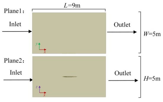
Figure 3.
Flow field of the telescoping wing.
The aerodynamic simulations employ a locally refined polyhedral mesh to enhance computational accuracy and optimize boundary layer resolution. The mesh resolution is adjusted to ensure that the dimensionless wall parameter y+ remains below 1, and a low-Reynolds-number wall treatment is adopted to enable full resolution of the viscous sublayer. The total number of mesh elements is approximately 1 × 10⁶, with the wing mesh element size set to 10−2 m. The height of the first-layer boundary layer mesh on the wing surface is set to 9 × 10⁻⁶ m, with a growth rate of 1.2 to ensure smooth mesh transitions.
In hypersonic flow conditions, the temperature distribution on the wing surface is influenced by viscous dissipation heating of the surrounding gas. Therefore, as illustrated in Figure 4, local mesh refinement is applied near the fluid–solid interface in the aerodynamic model to enhance computational accuracy and ensure high-quality boundary layer resolution.
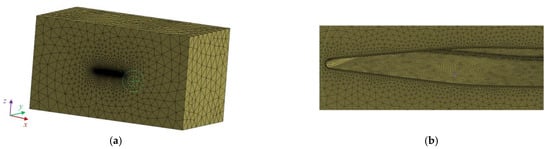
Figure 4.
Flow field meshing. (a) Global grid; (b) local grid.
After completing the flow field mesh division, the aerodynamic simulation solver and boundary conditions are configured. The most commonly used turbulence models in CFD analysis include the Spalart–Allmaras, k-ε, and k-ω models. Among these, the SST k-ω two-equation model combines the strengths of the k-ε model for free-stream flow and the k-ω model for near-wall flow by utilizing a blending function. This capability makes it particularly suitable for simulating large flow separations. The SST k-ω turbulence model is selected for solving the flow field.
Regarding boundary conditions, the inlet is set as a pressure far-field boundary with a static pressure of 5.5293 kPa, a temperature of 216.85 K, and an angle of attack of 5°. The outlet static pressure is set identical to the inlet. The wall boundary condition is modeled as an adiabatic no-slip wall. Given the influence of compressibility and thermal effects in the hypersonic flight environment of the multi-stage telescopic wing, the energy equation and compressible flow solver are activated in the simulation to ensure the accuracy of the computational results.
In ANSYS2021, the numerical solution of continuous problems relies on the finite element method (FEM), which discretizes the computational domain and approximates the distribution of unknown variables using a finite number of basis functions. First, the computational domain is established based on the geometric and physical characteristics of the study object. In the context of continuum mechanics, physical quantities are governed by partial differential equations. The weighted residual method is employed, and the Galerkin method is used to select appropriate interpolation functions, transforming the governing equations into an equivalent variational form, which is then approximately solved within finite elements. The computational domain is discretized into a finite number of elements, with variables defined at the nodes of each element. These variables are interpolated using shape functions to ensure continuity across the computational domain. After applying the appropriate boundary conditions, the discretized finite element equations are solved numerically to obtain the distributions of pressure, temperature, and other physical quantities, which are subsequently visualized for further analysis. In the static structural analysis, we adopted linear analysis under the small deformation assumption to ensure computational efficiency and solution convergence. For the driving force analysis, due to the presence of frictional contacts at multiple connection points, we employed a multi-step iterative method to solve the nonlinear problem. The time step was determined using the automatic time-stepping method (bisection approach) to ensure convergence at each computational step. Regarding mesh generation, considering the geometric complexity of some components and to avoid generating degenerate hexahedral elements, we used tetrahedral elements (Solid187). During structural simulations, the mesh size was set to 2 mm, resulting in approximately 1.5 × 10⁶ elements, which ensures sufficient computational accuracy and stability. The material model was defined according to the parameters listed in Table 1, while detailed descriptions of the boundary conditions, loading methods, and contact settings are provided in the corresponding analysis sections.
2.1.2. Aerodynamic Simulation Analysis
After establishing the flow field model, a systematic mesh convergence analysis is conducted to ensure that the computational results remain independent of mesh size. The primary objective of the mesh convergence analysis is to assess the influence of mesh resolution on aerodynamic force calculations and to determine the optimal mesh size that balances computational accuracy and efficiency. Therefore, all model parameters remain unchanged, with only the mesh size being varied to analyze the convergence behavior of lift and drag forces. In this study, a mesh size of 10−2 m is selected as the reference medium-resolution grid. Additionally, two finer mesh configurations and two coarser mesh configurations are generated to evaluate the effect of mesh refinement on computational accuracy.
Figure 5 illustrates the variations in lift and drag forces as a function of mesh size. The results indicate that as the mesh resolution increases, the computed values of lift and drag gradually converge. When the mesh size is further refined below 10−2 m, the numerical error is reduced to less than 0.2%, indicating that the computational discrepancy is within an acceptable threshold. Considering both numerical accuracy and computational cost, a mesh size of 10−2 m is deemed optimal, as further refinement has a negligible impact on the results. Thus, this study adopts a mesh size of 10−2 m to ensure computational accuracy while maintaining efficiency.
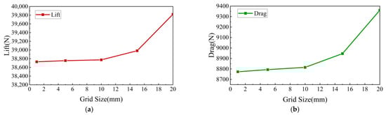
Figure 5.
Grid convergence analysis. (a) Lift variation; (b) drag variation.
The analysis is performed under the design flight conditions of Mach 5.0 at an altitude of 20 km. The aerodynamic and thermal loads on the wing are evaluated for these conditions. The wing’s aerodynamic and thermal load distribution contour maps are shown in Figure 6. As illustrated in Figure 6a, the wing surface pressure is predominantly within the range of 15 kPa.
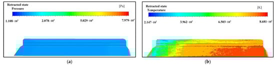
Figure 6.
Wing surface load aerodynamic simulation contour map. (a) Force load; (b) thermal load.
From the aerodynamic thermal load contour map of the wing surface shown in Figure 6b and the corresponding simulation dataset, the thermal load distribution of the wing is presented in Figure 7. Due to the impact effects of high-speed airflow and aerodynamic heating, the leading edge of the wing exhibits a higher temperature, reaching up to 600 °C. The temperature across the wing surface varies between 300 °C and 500 °C. The majority of the wing surface shows a relatively uniform temperature distribution, with temperatures stabilizing around 500 °C. This indicates that the aerodynamic heating effects rapidly diminish toward the rear part of the wing surface, and the thermal environment in most areas remains relatively stable. Based on these temperature distribution characteristics, to ensure representativeness and coverage during thermal experiments, the temperature of 500 °C, representative of the majority of the wing surface area, should be selected as the test criterion.
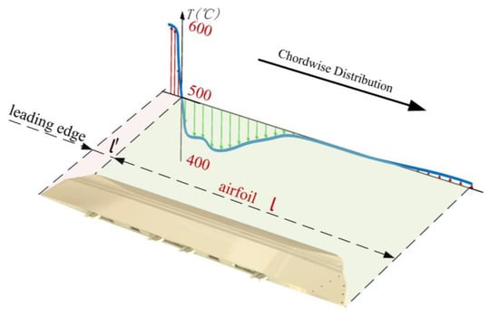
Figure 7.
Chordwise distribution of thermal load on wing surface.
Based on the aerodynamic simulation results of the service environment loads for the multi-stage telescopic wing, it is recommended to use an aerodynamic load of 15 kPa and an aerodynamic heating temperature of 500 °C as the evaluation conditions to simulate extreme flight scenarios. This selection not only simplifies the experimental conditions but also effectively covers the primary heat-affected regions of the wing surface under actual operating conditions, ensuring that the experimental results hold significant engineering relevance and practical guidance value.
2.2. Simulation Analysis of Deformation Process of Multi-Stage Telescopic Wing
To evaluate the deformation characteristics of the multi-stage telescopic wing under the prescribed loading conditions and verify the feasibility of its structural design, a simulation analysis was conducted to investigate its deformation behavior during the deployment process. The simulation model is illustrated in Figure 8, where a fixed constraint is applied at the wing root, and three distinct loading conditions are imposed on the skin surface: (1) aerodynamic loading only, (2) thermal loading only, and (3) combined force–thermal loading.
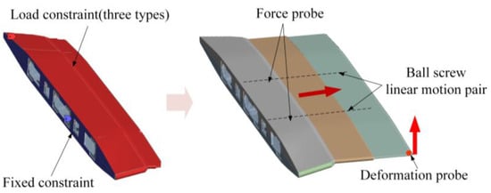
Figure 8.
Deformation process simulation model.
In the simulation setup, the contact interactions between the wing surfaces and moving components are defined as frictional contact, while rigidly connected regions are set as bonded contact. To precisely capture the structural response, a Z-direction deformation probe is placed at the intersection of the wingtip trailing edge and chordwise direction, while a force probe is embedded at the lead screw joint. Additionally, the displacement input of the lead screw is prescribed to simulate the transition of the multi-stage telescopic wing from a fully retracted state to a fully deployed state. The deflection of the wingtip and the driving force are subsequently recorded and analyzed to investigate the deformation behavior and mechanical characteristics of the structure.
Under the evaluation load conditions, a simulation analysis of the deformation process of the multi-stage telescopic wing was conducted to assess the feasibility of the structural design based on its deformation performance during deployment. In the simulation, fixed constraints were applied at the root of the wing, and three loading conditions were defined: (1) aerodynamic load only, (2) thermal load only, and (3) combined aerodynamic and thermal loads. Figure 9 illustrates the simulated tip deflection curves of the multi-stage telescopic wing under these three loading conditions during deployment. The results show that the deflection changes are smooth throughout the deployment process, with no sudden transitions, indicating that the structure’s response to combined aerodynamic and thermal loads is stable. This preliminary analysis validates the load-bearing capability of the multi-stage telescopic wing.
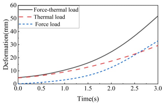
Figure 9.
Simulation of deflection deformation during the telescoping process.
Figure 10 shows the time-dependent curves of the driving force required for the deployment of the telescopic wing under three loading conditions. The driving force under coupled aerodynamic and thermal loads is significantly higher than that under aerodynamic loads alone. The driving force under thermal loads alone is nearly identical to that under coupled aerodynamic and thermal loads. This indicates that the driving force in the coupled condition is primarily influenced by thermal loads, and the impact of aerodynamic loads on the driving force is negligible in the presence of thermal loads.
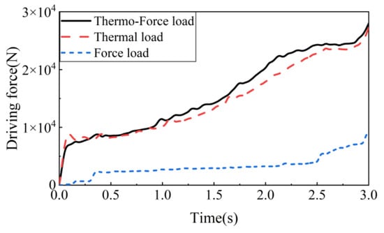
Figure 10.
Driving force under different operating conditions.
Table 3 shows the peak values of deformation and driving parameters during the unfolding process of the telescoping wing under three different conditions, based on simulation measurements. Through the analysis of the deformation curve and the driving force variation curve, it is observed that the deformation curve exhibits a smooth and continuous trend, while the driving force variation curve shows no abrupt fluctuations or sudden changes. This indicates that the mechanism can operate stably under the investigated conditions, with no noticeable discontinuities or unexpected transient behaviors during its motion. These findings fully demonstrate the actuation stability of the mechanism under force–thermal coupling effects, further supporting the rationality of its structural design and providing strong validation for its engineering application in complex loading environments. However, to ensure the reliability and practicality of the design, further ground simulation experiments under the assessment load conditions are necessary to complete the full verification of the structural design.
Table 3.
Peak values of measurement parameters.
3. Dynamic Force–Thermal Follow-Up Loading Method for Multi-Stage Telescopic Wings
3.1. Design of the Force–Thermal Follow-Up Loading Platform
To conduct force–thermal follow-up loading experiments under assessment conditions for deformable wings and enhance the experimental efficiency, this study proposes a design for a force–thermal follow-up loading platform for multi-stage telescopic wings of aircraft. As illustrated in Figure 11, the system comprises a multi-stage telescopic wing prototype, thermal load application units, force load application units, a supporting platform, and an associated control system. The telescopic wing prototype is mounted on the supporting platform, while the modular thermal and force load units are installed at predesignated positions on the wing surface, aligned with the prototype’s movement direction. A dynamic multi-point distribution equivalence method based on grid reconstruction is proposed to simulate aerodynamic loads. This method equivalently transforms the varying aerodynamic loads during motion into time-varying loads at predefined loading points, enabling follow-up loading throughout the entire process. Both the thermal and force load units are equipped with sensors, such as load cells and thermocouples, to collect real-time loading state data. These sensors connect to the control system, which provides feedback regulation to ensure that the experimental loads accurately follow the predefined loading conditions.
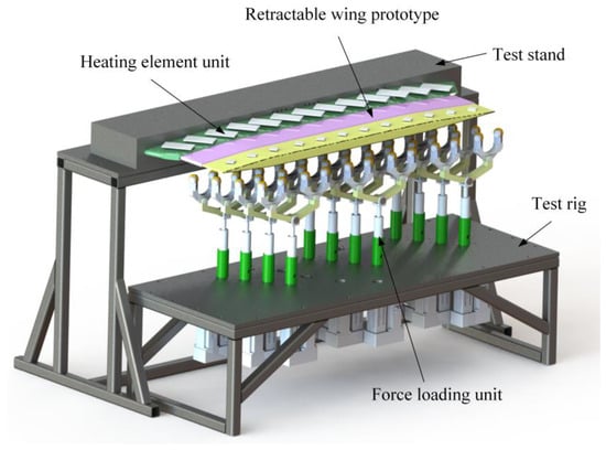
Figure 11.
Telescopic wing force–thermal follow-up loading platform.
A load unit design analysis is conducted for the multi-stage telescopic wing. Given that the force distribution along the chordwise direction of the wing is nearly uniform, the telescopic wing can be equivalently modeled as a cantilever beam along the spanwise direction, as illustrated in Figure 12. In this equivalent model, the wing root is assumed to be fixed, while the other end remains free. Corresponding cantilever beam models are established to analyze the structural response under both aerodynamic and concentrated loads.
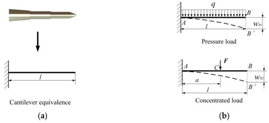
Figure 12.
Establishment of the cantilever equivalent model for multi-stage telescopic wings. (a) Cantilever equivalence; (b) equivalent model under different loads.
When the equivalent model is subjected to a uniformly distributed pressure load q, the deflection at the free end (point B), denoted as wB1, is given by the following Equation (1):
where l represents the wingspan, E is the elastic modulus of the material, and I is the moment of inertia of the cross-section.
When the equivalent model is subjected to a concentrated load F, the deflection at the free end (point B), denoted as wB2, is given by the following Equation (2):
where a represents the distance from the fixed end to the point of load application.
As the number of concentrated loads increases, the accuracy of simulating the uniformly distributed load improves progressively. As shown in Figure 13, with an increasing number of concentrated loads, the distribution characteristics of shear force and bending moment in the equivalent model more accurately approximate those under a uniformly distributed load. This indicates that increasing the number of concentrated loads within a reasonable range enhances the accuracy of equivalent modeling, thereby providing a more precise representation of the effects of a uniformly distributed load on the structure.
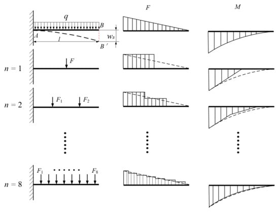
Figure 13.
Deflection variation under different numbers of concentrated loads.
Figure 14 illustrates the variation in deflection error at the free end as the number of equivalent concentrated loads increases. The results indicate that when the number of spanwise concentrated load points reaches four or more, the error reduction rate falls below 2%. Additionally, within the range of [4,8] concentrated load points, the equivalent loading error remains below 10%. When the number of spanwise concentrated loads reaches four or more, further increasing the number of concentrated loads reduces the deflection fitting error by less than 2%. Therefore, arranging four or more spanwise loading units meets the acceptable error requirements. Considering the design constraints of the actual drive sources and installation space, four spanwise loading units are selected as the final design configuration.
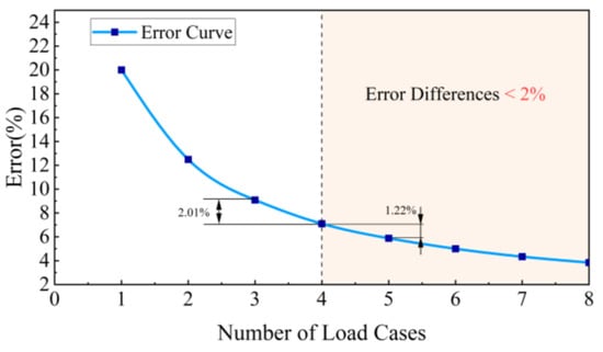
Figure 14.
Variation in error with the number of concentrated loads.
The number and positions of chordwise loading points are determined through comparative simulation analyses. As shown in Figure 15, the deformation of 10 characteristic nodes in the fully extended state of the telescopic wing is used as the basis. With 4 spanwise loading units, 4 comparative simulations were conducted for chordwise loading point counts of 3, 6, 9, and 12. These simulations evaluate the deflection deformation under uniformly distributed pressure loads acting on the wing surface. All finite element models were configured identically, differing only in the number of chordwise loading points applied to the wing. The simulation results, presented in Table 4, indicate that when 36 or more loading points are used, further increases in the number of loading points result in error reduction rates of less than 0.5%. Consequently, 48 loading points are selected as the final configuration.
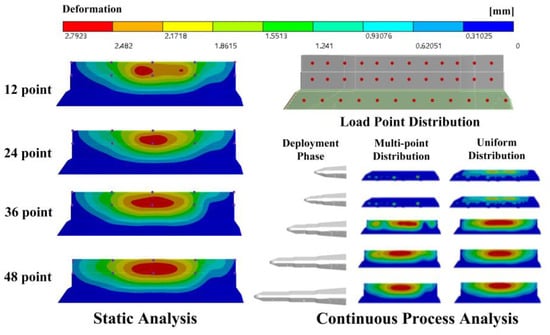
Figure 15.
Simulation analysis of load point positions.
Table 4.
Fitting errors under different numbers of concentrated loads.
Based on the design of modular loading units, the aerodynamic loads acting on the wing surface during follow-up loading need to be equivalent to time-varying concentrated loads at predefined loading points. This paper proposes a dynamic multi-point distribution equivalence method for aerodynamic loads, introducing dynamic grid reconstruction to achieve equivalent load simulation under minimum strain energy conditions. Taking the equivalent model of the multi-stage telescopic wing as an example, a grid sensitivity analysis of this method was conducted. The proposed load simulation method was then applied to map the assessment loads onto predefined loading points, resulting in load curves for each loading point throughout the loading process. These results were compared with those obtained using the traditional empirical equal-division method. Finally, an equivalent control system model for the loading units was established. Mechanical and control system models of the designed force–thermal follow-up loading platform were built in simulation software, and simulation analyses were conducted to verify the loading system’s response capabilities.
3.2. Dynamic Multi-Point Distribution Equivalence Method for Aerodynamic Loads
Existing research on load equivalence methods for loading experiments primarily relies on empirical methods, such as equal-area averaging. These methods divide the wing surface into multiple equal-area regions and distribute the aerodynamic loads across these regions, approximating them as concentrated loads to satisfy static equivalence conditions. In contrast, this study adopts the commonly used multi-point distribution method for mapping aerodynamic loads to structural grid points. This method is extended to calculate load equivalence at loading points by incorporating dynamic grid reconstruction, thus proposing the dynamic multi-point distribution equivalence method, which achieves full-process equivalence of time-varying loads.
The basic concept of the multi-point distribution method is as follows: in finite element analysis, after obtaining the aerodynamic loads acting on the wing structure, these loads are mapped from the aerodynamic grid to the structural grid. This is necessary because the grids used for aerodynamic analysis and those for static structural analysis do not perfectly correspond. When the number of structural grid points is sufficiently small, they can be regarded as predefined equivalent loading points.
As shown in Figure 16, given the position coordinates and corresponding loads of i × k aerodynamic grids on a certain wing surface, the goal is to equivalently transfer all aerodynamic grid loads to predefined loading points{(xk, yk), k = 1, 2, 3, …, n}. Taking a particular aerodynamic grid as an example, consider the aerodynamic load po acting on the grid at point o(xu, yq). It is assumed that all the predefined loading points and the aerodynamic grid o are connected by a virtual beam (of length lk), and they both act as cantilever beams with the fixed end at point o. The deformation energy when the load pk is applied to the loading point is as follows:
where EJ represents the bending stiffness of the virtual beam element.
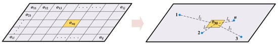
Figure 16.
Schematic of the multi-point distribution method.
The loads distributed to each structural point should satisfy the following static equilibrium condition:
where k represents the kth loading point, with its value ranging from 1 to n, while n denotes the total number of loading points.
The Lagrangian function is constructed using the method of Lagrange multipliers, as follows:
where , , and are the Lagrange operators for the static equivalent condition construction function, represents the difference in the x-coordinate between loading point k and the aerodynamic grid, and represents the difference in the y-coordinate between loading point k and the aerodynamic grid.
Taking the derivative and setting it equal to zero yields the following:
By combining Formula (3), we can obtain the following:
By solving λ and substituting it into Equation (4), the aerodynamic load of each aerodynamic grid point ouq (u = 1, 2, 3, …, i; q = 1, 2, 3, …, j) is distributed to the corresponding structural grid points. Using the above method, the aerodynamic loads on the wing surface are equivalently allocated to the predefined structural grid points.
The above multi-point distribution method completes the load equivalence of aerodynamic grid loads on the wing surface to the predefined loading points at a specific moment. Building on this, a dynamic multi-point distribution method is proposed by incorporating the mesh reconstruction technique, enabling time-varying loads with changing areas to be equivalently distributed to fixed predefined loading points.
The dynamic multi-point distribution method operates as follows: The entire motion process is discretized into a finite number of time steps at regular intervals, converting the dynamic process into a series of quasi-static processes. At each time step, the aerodynamic grid on the wing surface is re-meshed to achieve dynamic grid updates. The multi-point distribution method is then applied at each time step to allocate the aerodynamic grid loads to the predefined loading points. The loads throughout the discretized process are interpolated and fitted, resulting in the load distribution across all loading points during the motion. This distribution ensures that the equivalent conditions of force and moment are satisfied at all times while minimizing the additional strain energy introduced by load equivalence.
As shown in Figure 17, during the wing deformation process, the entire process is discretized into t1 to tn, representing n finite moments. At each moment, the wing profile undergoes dynamic grid updates. The selection of the time step Δt depends on the adopted time discretization strategy, which is typically determined based on the maximum wave speed of the material cmax and the minimum mesh size Lmin. In this study, the Courant–Euler–Lagrange (CEL) stability condition is applied, as follows:
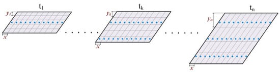
Figure 17.
Discretization of the dynamic multi-point distribution method.
This condition ensures the numerical computation remains stable and accurate, allowing for the precise capture of dynamic physical phenomena. To guarantee that the simulation results accurately reflect the real-world physical process, the time step Δt in numerical simulations should be consistent with the characteristic timescale of the physical process.
During the deformation process of the multi-stage telescopic wing, the spanwise length dynamically changes with the deployment state, necessitating an investigation into the influence of mesh size on computational convergence. To address this issue, this study proposes a mesh update strategy based on a fixed total number of mesh elements, ensuring uniformity in mesh distribution throughout the simulation and preventing errors caused by uneven mesh sizes. Since planar meshing is employed in this study, maintaining a constant mesh size across different deployment states would result in varying mesh densities in different regions, potentially affecting computational accuracy. Therefore, instead of fixing the mesh size directly, a strategy of maintaining a constant total number of mesh elements along a specific direction is adopted. This allows the mesh size to adapt dynamically to changes in the spanwise dimension, ensuring consistent meshing across different deformation states. By analyzing the error variations in aerodynamic load calculations under different mesh element counts, the minimum required mesh number for achieving computational convergence is determined. This approach not only guarantees mesh consistency under varying deformation states but also enhances computational efficiency by avoiding unnecessary over-refinement, thereby improving the overall stability and reliability of the numerical simulation.
The sensitivity analysis is performed at the state of t1, with a total of 12 loading points acting on the wing surface. Sensitivity to grid quantity is analyzed separately for chordwise and spanwise directions. The first analysis examines the influence of chordwise grid quantity, and the second analysis examines the influence of spanwise grid quantity.
- (1)
- Sensitivity Analysis of Chordwise Grid Quantity
The initial value of the spanwise grid quantity is set to 100, and the chordwise grid quantity is increased from 5 to 300 in increments of 5 to analyze the changes in the load equivalence at the 12 loading points, as shown in Figure 18. The results indicate that the loading force at each unit becomes nearly unaffected by further increases in the grid quantity once it exceeds 50.
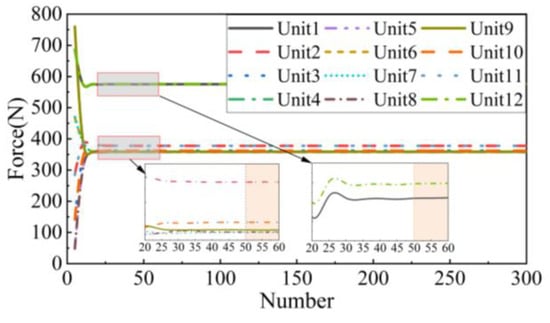
Figure 18.
The effect of the chordwise grid quantity on the equivalent load.
- (2)
- Sensitivity Analysis of Spanwise Grid Number
The number of spanwise grids is initially set to 50, and the spanwise grid number is increased from 50 to 3000 in increments of 50. The variations in the load equivalence at 12 loading points are analyzed, as shown in Figure 19. The loads with significant variations, after the number increases to 1500 or more, show an absolute error of less than 0.2 N when compared to the final convergent value. The force load distribution is almost no longer affected by the change in the number of grids.
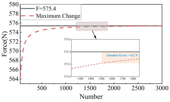
Figure 19.
The effect of the spanwise grid quantity on the equivalent load.
Based on the grid sensitivity analysis, the increase in grid number has a certain impact on the load equivalence results. However, once the grid number reaches a certain threshold, the change in grid number has minimal effect on the load equivalence results. Therefore, the grid update method for each moment is to keep the grid unchanged based on a certain number. The chordwise grid length remains unchanged as the wing does not deform in the chordwise direction, while the spanwise grid length gradually increases. In subsequent analyses, the grid reconstruction number is determined to be 50 for the chordwise direction and 1500 for the spanwise direction. In this study, the minimum mesh size Lmin is determined to be 0.107 mm, while the maximum wave speed of the selected material GH4169 is calculated as 4901.781 m/s. Consequently, based on the CEL condition, the time step Δt required to maintain computational stability is calculated as follows:
3.3. Method Comparison and Validation
3.3.1. Load Calculation
In existing research, a commonly used load equivalence method is to divide the wing surface into multiple equal-area regions, set loading points, and directly distribute the loads based on the total force acting on the wing surface, using the equal-area allocation method. Equation (10) is as follows:
where P represents the pressure load acting on the wing, S denotes the loaded area, and n indicates the number of equally divided area sections. Fi represents the load value assigned to the i-th loading point.
That is, the wing surface is divided into multiple regions of equal area, with a loading point set in each region. The resultant force of the loads at multiple loading points, Fi, is equal to the total load acting on the wing surface, while the position design also considers the equivalence of the moment. This method can somewhat simulate aerodynamic loads that are relatively evenly distributed. However, when applied to complex and variable aerodynamic loads, this method struggles to achieve a good fit. Therefore, one advantage of the dynamic multi-point allocation method studied in this paper is its ability to fit and equivalently simulate complex aerodynamic loads on the wing surface with high accuracy. Similarly, when handling uniformly distributed aerodynamic loads, the method proposed in this paper still maintains a high level of fitting accuracy. Below, using the multi-stage telescopic wing equivalent model as the object, both methods will be applied to compare the fitting accuracy of wing surface load deformation trends to verify the superiority of the method studied in this paper.
First, the variation in wing surface loads during the entire telescopic process of the multi-stage telescopic wing under the 15 kPa test load will be analyzed. When the multi-stage telescopic wing extends, the extension speed is constant, and the change in area per unit time is a fixed value. Under the pressure load, the aerodynamic load on the wing surface increases linearly. The fixed wing area remains constant, while the middle and outer wings extend synchronously. The resultant forces on each wing surface, i.e., Ff, Fm, and Fo, are as follows:
where Sf refers to the loaded area of the fixed wing, Sm denotes the loaded area of the intermediate wing, Sm1 represents the initial loaded area of the intermediate wing, lm is the chord length of the intermediate wing, So refers to the loaded area of the outer wing, So1 represents the initial loaded area of the outer wing, lo is the chord length of the outer wing, and v is the extension speed.
The total aerodynamic force F acting on the wing surface is as follows:
The change curve of the total force acting on the wing surface is shown in Figure 20.
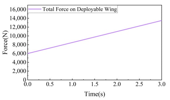
Figure 20.
The change curve of the total force acting on the telescoping wing.
The aerodynamic load equivalence distribution is performed using both the traditional equal-area division method and the dynamic multi-point allocation method. The results are shown in Figure 21 and Figure 22, respectively.
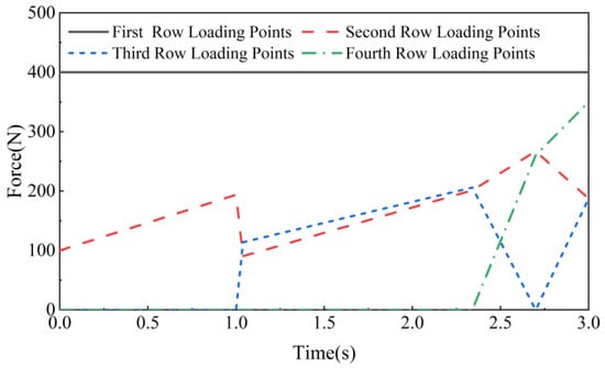
Figure 21.
Time-varying force curve for loading points using the equal-area allocation method.
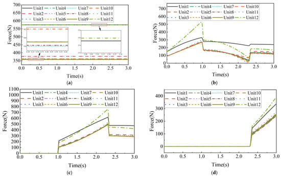
Figure 22.
Load curve allocated by the dynamic multi-point distribution method. (a) Time-varying force curve for the first set of loading points; (b) time-varying force curve for the second set of loading points; (c) time-varying force curve for the third set of loading points; (d) time-varying force curve for the fourth set of loading points.
3.3.2. Initial Moment Analysis and Validation
After obtaining the load distribution from both methods, a comparison analysis was conducted by simulating the deformation trend of the wingtip deflection under the equivalent loads and comparing the fitting degree with the aerodynamic load. The constraints for the initial moment analysis at 0 s are shown in Figure 23. The root of the equivalent wing was fixed, and simulations were carried out under the following three load conditions on the wing surface: ① the evaluation aerodynamic load, ② the equal-area distribution load, and ③ the dynamic multi-point allocation method equivalent load.
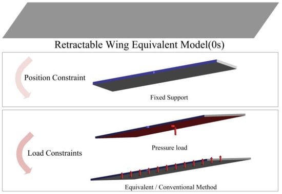
Figure 23.
Simulation constraints.
The initial moment data of the three load cases were input into the simulation model to obtain the simulation results, as shown in Figure 24. The wingtip deformation trajectories were extracted from the three results to analyze the fitting effects of different equivalent methods and aerodynamic loads. Figure 25 shows the extracted wingtip deformation trajectories under the three loading conditions.
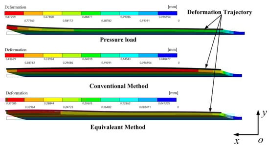
Figure 24.
Simulation wingtip trajectory.
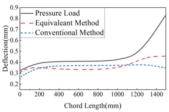
Figure 25.
The 0 s wingtip deformation trajectory.
To comprehensively evaluate the fitting performance of the proposed dynamic multi-point allocation method and the traditional equal-area allocation method in practical applications, this paper calculates two commonly used error metrics, namely root mean square error (RMSE) and the coefficient of determination (R2), for comparative analysis. RMSE is primarily used to measure the magnitude of fitting errors between the two methods, giving higher penalties to larger errors. R2, on the other hand, reflects the correlation between the model’s calculation results and actual values, indicating the model’s ability to explain data variability. Through the joint analysis of these two metrics, the fitting performance of the model can be more comprehensively assessed.
The root mean square error (RMSE) is a metric used to measure the difference between the fitted values and the true values. It is defined as the square root of the average of the squared differences between the fitted and actual values, as follows:
where ypred,i is the equivalent value for the i-th sample, ytrue,i is the aerodynamic load value, and n is the number of samples in the dataset. A smaller RMSE value indicates that the difference between the model’s fitting results and the actual results is smaller, meaning the fitting performance is better.
The coefficient of determination R2 measures the correlation between the model’s computed values and the actual values. Its formula is as follows:
where is the mean of the actual values. The R2 value ranges between 0 and 1, with a value closer to 1 indicating a stronger ability of the model to explain the data variability and a better fitting performance. This paper evaluates the superiority of the fitting performance of the two methods by comparing their performance based on RMSE and R2 metrics.
For the error analysis of the two methods at the initial state, RMSE and R2 values were calculated using the wingtip deflection simulation trajectory data. The fitting error results for the dynamic multi-point allocation method and the equal-area distribution method at the initial moment are shown in Table 5.
Table 5.
Fitting error at the initial moment.
The results show that, at the initial moment, the dynamic multi-point allocation method proposed in this paper outperforms the equal-area distribution method in both metrics. Specifically, the smaller RMSE indicates a better fitting effect, while the R2 value close to 1 for the dynamic multi-point allocation method indicates its excellent fitting performance, which is capable of explaining the variability in the data well.
3.3.3. Continuous Process Analysis and Validation
In practical load equivalence applications, the telescoping wing undergoes a continuous deformation process, requiring the equivalent aerodynamic loads to be applied throughout the entire process. During the equivalence, the entire process is discretized into a finite number of time instances, and the equivalent time-varying load curve for the whole process is fitted. To compare the dynamic process, the method proposed in this paper is contrasted with the traditional empirical method. Several typical working conditions during the entire process are selected for dynamic process comparison, as shown in Table 6. The selected working conditions include moments when the number of loading points changes and intermediate instances.
Table 6.
Typical operating conditions.
For different operating conditions, comparative simulation models are established, with the same constraints as described in the previous section. The load data at different time instances are input into the simulation model, and the results are obtained. The wingtip deformation trajectories are extracted from the three sets of results to analyze the fitting effects of different equivalence methods under aerodynamic load conditions. Figure 26 shows the extracted wingtip deformation trajectories under the three loading conditions at different time instances.
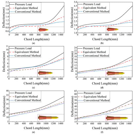
Figure 26.
Wingtip deformation trajectories for various conditions. (a) Wingtip deformation trajectory at 0.1 s; (b) wingtip deformation trajectory at 0.54 s; (c) wingtip deformation trajectory at 1.11 s; (d) wingtip deformation trajectory at 1.77 s; (e) wingtip deformation trajectory at 2.46 s; (f) wingtip deformation trajectory at 3 s.
The RMSE and R2 values are calculated using the wingtip deflection simulation trajectory data for each operating condition. The fitting error results for the dynamic multi-point distribution method and the area-based distribution method at each time instance are shown in Table 7.
Table 7.
Fitting errors at different moments.
Figure 27 visualizes the fitting error results at different time instances. From the figure, it can be observed that the dynamic multi-point distribution method proposed in this study outperforms the area-based distribution method in both RMSE and R2 metrics at all time instances. In terms of RMSE, the dynamic multi-point method slightly outperforms the traditional method in the early stage and continues to maintain a lower error as the wing extends. Meanwhile, the R2 value of the dynamic multi-point distribution method starts at 0.84 and rapidly approaches 1, maintaining a value close to 1 throughout the wing extension. This indicates that, in the entire equivalence process, the dynamic multi-point method provides a better fit to the aerodynamic loads compared to the area-based method, demonstrating a stronger ability to adapt to the variation in the load.
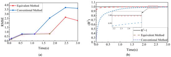
Figure 27.
Comparison of fitting errors. (a) RMSE; (b) R2.
From the above comparative analysis, it is evident that the two error metrics, namely RMSE and R2, evaluate the methods from different perspectives. RMSE focuses on the absolute difference between the fitted values and the actual values, with lower RMSE values indicating better performance in terms of absolute errors. On the other hand, R2 emphasizes the correlation between the fitted values and the actual values, with higher R2 values indicating that the method can better capture the variability in the data and has a stronger fitting capability.
Through the combined analysis of these two metrics, it can be observed that the area-based distribution method exhibits a relatively high RMSE and a lower R2 value. This suggests that the area-based method may not fully capture the variation in the load distribution in certain cases or that it may involve a significant fitting error. In contrast, the dynamic multi-point distribution method proposed in this study shows better fitting performance, particularly in terms of smaller errors and higher fitting accuracy.
3.4. Force–Thermal Follow-Up Loading System Modeling and Simulation Analysis
To ensure that each force loading unit can apply the preset force–load curve, a force feedback control system is designed for real-time feedback control of the loading unit’s force. The loading units are organized into a modular system, so an equivalent system model is established for a single loading unit. Figure 28 shows the equivalent impedance control model of the loading unit. The servo cylinder in the follow-up loading unit is simplified and equivalent to a moving slider with the mass md, with the driving input F(t) and displacement x1(t). The loading unit and the deformed wing surface are considered to be in constant contact during the loading process. kd is the equivalent stiffness of the disc spring in the loading unit, and cd is the system’s equivalent damping. The theoretical model for the follow-up loading unit is established as follows:
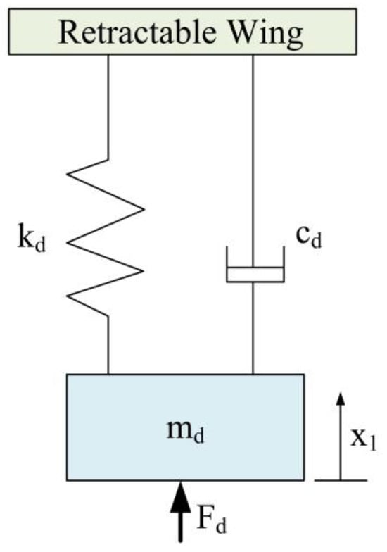
Figure 28.
Impedance control model.
Taking the Laplace transformation of Equation (13), the expression is obtained as follows:
Equation (14) represents the transfer function of the moving slider displacement x1 corresponding to the driving input force F in the deformable wing tracking loading control system, as follows:
Based on the transfer function from Equation (19), the control program block diagram of the tracking loading system is provided, as shown in Figure 29. The input force Fd serves as the system input, and the equivalent spring force F during the tracking process is the output, which is fed back to the PID controller. The PID controller adjusts the tracking loading unit to ensure the output force follows the desired force. The output of the PID algorithm is shown in Equation (16):
where F(t) is the output of the controller; e(t) is the response error; and Kp, Ki, Kd are the coefficients for the proportional, integral, and derivative terms, respectively.
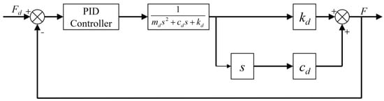
Figure 29.
Block diagram of the control system.
According to the design scheme of the force–thermal follow-up loading platform, a mechanical system model was established and imported into ADAMS2020. The material properties of each component were defined, appropriate motion pairs and contacts were added at the joints, and the corresponding driving conditions were applied to construct the loading platform mechanical system, as shown in Figure 30. Combining the established control system model, a control system simulation program block diagram was built. The integrated simulation of the follow-up loading platform with force feedback control was conducted to analyze the loading force error and the stability of the control system.
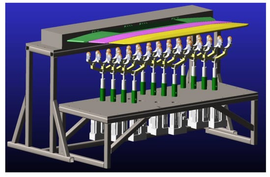
Figure 30.
Mechanical system model.
Figure 31 shows the entire process of dynamic loading. The twelve force loading units of the dynamic loading platform are divided into four rows, with three loading units in each row. The loading units in the same row act on the same section of the wing surface. For the analysis of the loading process, the four rows of loading units are taken as an example from the side view. The dynamic loading process is as follows: In the initial state, the four rows of loading units are positioned away from the external surface of the telescoping wing. During the loading process, the first two rows of loading units apply force to the telescoping wing. As the wing extends, the resultant force from the loading units acting on the wing increases. When the wing extends to the position of the third row of loading units, the third row of loading units rises and makes contact with the external surface of the wing, applying force. Similarly, when the wing extends to the position of the fourth row of loading units, the fourth row of loading units rises to make contact and applies force. This process continues until the wing is fully extended. During retraction, the process is reversed. When the telescoping wing retracts to the corresponding loading unit position, the loading units separate from the wing surface until complete retraction is achieved.
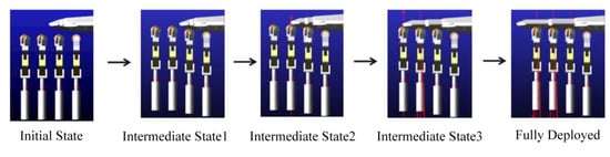
Figure 31.
Follow-up loading process of the multi-stage telescopic wing.
During the dynamic loading process, the resultant force applied by the loading points is equivalent to the resultant force acting on the wing under a uniform pressure load. The load–time curve for each loading unit throughout the entire process can be determined based on the position of each row of loading units and the extension speed of the telescoping wing. The force feedback control system program for each loading unit is shown in the figure. The program mainly adopts the PID control method, specifying the force curve for each loading unit, so that the force feedback control system can apply the specified force to the wing surface of the telescoping wing.
The feedback curve for the given force curve in the force feedback control system is shown in Figure 32. For a constant force loading system, force control follow-up can be achieved within 0.2 s. For time-varying loads, the loading system can also achieve load follow-up within 0.4 s with good accuracy. Simulation analysis shows that the loading error is within 1%. As seen in the figure, during the deformation process, the applied loading force can stably follow the input force curve.
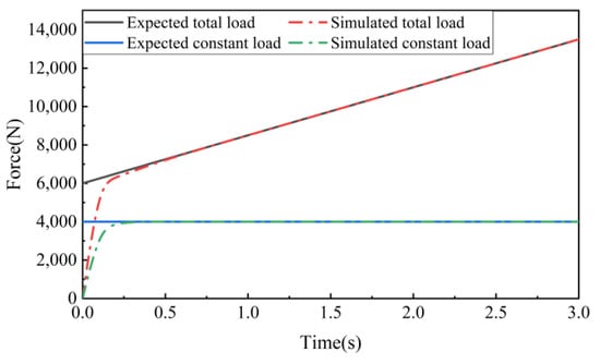
Figure 32.
Load tracking simulation results.
4. Experimental Verification
To validate the practical effectiveness of the proposed method and assess its applicability in real-world scenarios, this study evaluates the accuracy and reliability of the method by comparing the experimental results with the simulation data. The consistency of trends between the experimental and simulation data serves as a critical measure of the method’s performance in replicating actual conditions. A force–thermal loading experiment was conducted on a multi-stage telescopic wing to verify the method. The study compared the dynamic deflection curves and driving force variations under force–thermal loads with their corresponding simulation results. Error metrics were calculated to quantitatively analyze the differences. Figure 33 illustrates the experimental setup for the force–thermal loading system. The primary components include a prototype of the multi-stage telescopic wing, the force–thermal loading unit, ceramic heating elements, and a laser displacement sensor.
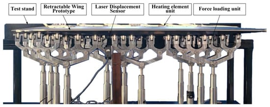
Figure 33.
Multi-stage telescopic wing force–thermal follow-up loading platform.
4.1. Force Load Regulation Experiment
First, experimental testing was conducted on the force loading system to evaluate its PID regulation and load-following capability under constant and time-varying load conditions. Since the follow-up loading system is composed of multiple units, the response of a single unit was tested. To verify the system’s response and tracking performance, a constant force of 4000 N and the equivalent calculated time-varying total load were set as the predefined input forces. The loading system was activated to test the response of the follow-up loading unit to the input forces.
As shown in Figure 34, the blue curve represents the experimental response of the loading force. Throughout the motion process, the experimental response oscillates slightly around 4000 N. An error analysis comparing the experimental and simulation results reveals a maximum load error of 208.4 N. The system’s response speed is also within 0.2 s, indicating that the load following is achieved within a short response time, with the experimental error remaining within 5% of the simulation values. The experimental data show fluctuations in the force load, likely caused by precision errors in the servo motor controller. Overall, the experimental response curve aligns with the simulation response curve in terms of trends, and the error is within an acceptable range.
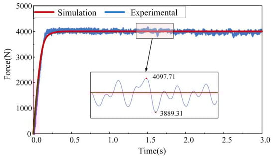
Figure 34.
Constant force load regulation experiment.
When the pre-applied load is changed to a time-varying load, Figure 35 shows the load-following behavior. The loading system rapidly achieves load following, similar to the constant load case, within 0.4 s, with the maximum loading error remaining under 5%. This further verifies the accuracy of the theoretical and simulation analyses, as well as the responsiveness of the force–thermal follow-up loading platform.
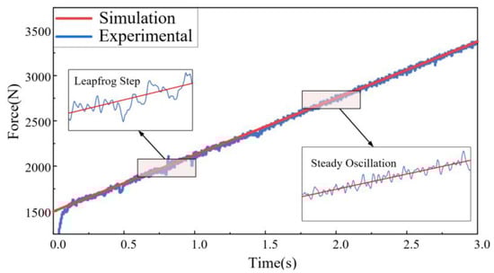
Figure 35.
Time-varying force load control experiment.
4.2. Force–Thermal Follow-Up Loading Experiment
4.2.1. Deflection Deformation Experiment
After completing the loading system capability tests, a force–thermal follow-up loading experiment was conducted on the multi-stage telescopic wing. The applicability of the loading method was analyzed based on the deflection deformation trend of the wingtip during the telescoping process.
The experimental conditions were set to be the same as the simulation analysis conditions described earlier. The evaluation conditions were set as follows: (1) only force load acting, (2) only thermal load acting, and (3) combined force and thermal loads acting. During the experiment, the force load was applied based on the time-varying distributed force load calculated using the dynamic multi-point equivalent method proposed in this study, and the thermal load was applied through conductive heating using the thermal loading unit. The wingtip deformation during the movement of the multi-stage telescopic wing was recorded under different loading conditions and compared with the simulation results. The comparison results of the experiment and simulation are shown in Figure 36 and Figure 37. The deformation trends of the wingtip under all loading conditions were similar to the simulation results, but the deformation trends in the experiment were somewhat larger than those in the simulation. The reason for this difference is that, during the actual installation of the experimental setup, there were certain installation gaps between components. This resulted in the loading time gaps, causing some motion in the wingtip, which led to a certain deformation error and, thus, a reduction in the stiffness in the experimental tests.
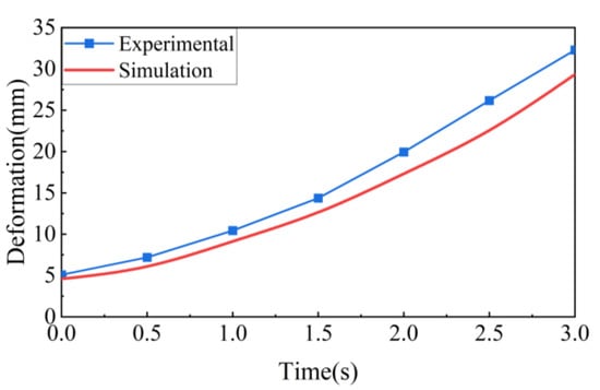
Figure 36.
Wingtip deformation versus time curve under thermal load only.
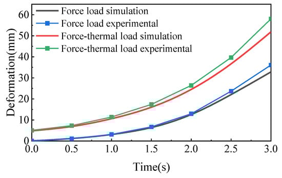
Figure 37.
Deflection change curves under force load only and under a combined force–thermal load.
Table 8 shows the maximum errors between the experimental results and the simulation results under various conditions. It can be seen that the maximum deformation errors are all within 10%. In all three cases, the RMSE values of deflection deformation are relatively small, and the R2 values are all above 0.9, which is close to 1. Both indicators suggest that the differences between the experimental and simulation results are minimal. The equivalent loads obtained using the dynamic multi-point distribution method can, to some extent, fit the wingtip deflection deformation behavior.
Table 8.
Deflection deformation errors.
4.2.2. Driving Force Experiment
Driving force experiments were conducted during the extension process of the telescopic wing under three different loading conditions. The experimental results were compared with the previously presented simulation model calculations for analysis. During the experiments, the force load was derived from the time-varying distributed load calculated using the dynamic multi-point distribution method proposed in this study, while the thermal load was applied through conductive heating using thermal loading units.
To evaluate the consistency between the experimental data and simulation results, this study presents a trend comparison of experimental and simulation outcomes under three different loading conditions. The driving force variation trends under the three loading scenarios are depicted in Figure 38.
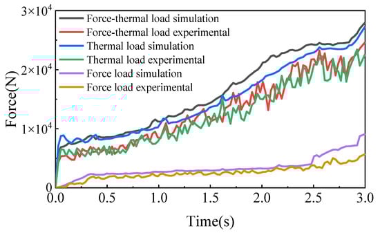
Figure 38.
Comparison of driving force under force–thermal conditions.
In all three cases, the experimental and simulation results exhibit generally consistent trends. However, the experimentally measured driving force is generally lower than the simulation data. The primary reason is attributed to the strict constraints applied in the simulation settings, which tightly restrict component deformation. This leads to significant differences in deformation across different regions, particularly under thermal loading conditions. Non-uniform deformation increases friction, resulting in higher driving forces in simulations. Conversely, during the experiment, installation gaps and errors allow for a certain degree of free thermal expansion deformation in various directions, reducing the required driving force to some extent. Nevertheless, the overall deformation trends under identical loading conditions remain consistent between the experimental and simulation results.
To quantitatively evaluate the consistency between the experimental and simulation results for driving force, two error estimation metrics were calculated: the root mean square error (RMSE) and the coefficient of determination (R2). Table 9 presents the error calculation results for the driving force. From the comparison between experimental and simulation results, all three loading conditions exhibited good trend consistency. In particular, under the force-only loading condition, the experimental and simulation results showed the highest agreement, with a small RMSE value and an R2 of 0.9508, indicating that the simulation model under force-only loading is highly accurate. However, under thermal loading and combined force–thermal loading, the discrepancies between the experimental and simulation results increased. Specifically, under force–thermal coupled loading, the RMSE value was larger, suggesting a decline in model prediction accuracy under multi-load coupling.
Table 9.
Driving force error.
In the experimental section, the response capability of the follow-up loading system was first tested, verifying its high follow-up response capability. Subsequently, experimental tests were conducted under three loading conditions, namely thermal load, force load, and combined force–thermal load, focusing on performance metrics, such as deflection deformation and driving force. These results were compared with simulation data. By calculating RMSE and R2, the fitting accuracy between experimental and simulation results was analyzed, validating the feasibility of the proposed force–thermal follow-up loading method and the correctness of the theoretical and simulation analysis.
5. Conclusions and Prospects
This study proposed a force–thermal follow-up loading method for multi-stage telescopic wings and investigated the dynamic multi-point distribution equivalence method for transferring aerodynamic loads to predefined loading points during dynamic processes. Comparison with the traditional equal-area distribution method demonstrated the significant advantage of the proposed method in accurately fitting wingtip deformation trajectories, achieving a full-process fitting accuracy with R2 >0.9. The research indicates that the proposed force–thermal follow-up loading method not only effectively achieves static loading, constant force–thermal follow-up loading, and time-varying force–thermal follow-up loading, but also exhibits good scalability, making it applicable to loading experiments for multi-dimensional morphing wings, such as telescopic folding and telescopic swept wings.
The theoretical model of the follow-up force loading system for multi-stage telescopic wings was derived in this study. Based on this model, simulation models of the follow-up force loading control system and mechanical system were established. Simulations verified that the system’s response capability reached within 0.4 s with an error margin of less than 1%, providing a theoretical foundation for the design and application of future loading systems.
A force–thermal follow-up loading platform for multi-stage telescopic wings was developed and utilized to conduct ground simulation experiments. Experimental results showed that the loading system achieved a response speed within 0.4 s, with a load-following error maintained within 10%. Additionally, a comparison of the experimental results of wingtip deflection deformation and driving force during the telescoping process revealed consistent trends with the simulation results, further validating the feasibility and effectiveness of the designed force–thermal follow-up loading platform and its simulation analysis.
This study proposes and validates the effectiveness of the dynamic multi-point row equivalence method in force–thermal follow-up loading experiments for multi-stage telescopic wings. However, to further enhance the applicability and accuracy of this method, the following research directions should be explored in the future: (1) optimization of the loading method: improving the arrangement of loading points and load distribution strategies based on experimental and simulation feedback to enhance load simulation accuracy. (2) Experimental studies under complex conditions: conducting comprehensive experiments under broader flight conditions, such as high-speed aerodynamic loads and non-uniform temperature fields, to improve the engineering applicability of the method. (3) Multi-physics coupling simulations: establishing high-precision simulation models that incorporate aero-structural and thermodynamic coupling for more accurate representations of actual flight conditions. (4) Expansion of engineering applications: promoting the application of this method in the structural optimization of morphing aircraft, thereby improving the engineering practicality of multi-stage telescopic wings.
These future studies will further refine the dynamic multi-point row equivalence method, enhance the accuracy of force–thermal follow-up loading experiments, and provide a solid theoretical and experimental foundation for the engineering application of high-performance morphing wings.
Author Contributions
Conceptualization, S.L.; methodology, S.L.; software, S.L.; validation, S.L.; formal analysis, S.L.; investigation, S.L.; resources, S.L.; data curation, S.L.; writing—original draft preparation, S.L.; writing—review and editing, S.L., H.L. and C.L.; visualization, S.L.; supervision, H.X., H.G. and J.T.; project administration, H.G.; funding acquisition, H.X., H.G. and G.Y. All authors have read and agreed to the published version of the manuscript.
Funding
This research has received grants from the National Natural Science Foundation of China (NSFC) through grants Nos. 52192633, T2388101, 52405013, and U2341237, and the China Postdoc-toral Science Foundation (No. 2023T160168).
Institutional Review Board Statement
Not applicable.
Informed Consent Statement
Not applicable.
Data Availability Statement
The original contributions presented in this study are included in the article. Further inquiries can be directed at the corresponding authors.
Conflicts of Interest
The authors declare no conflict of interest.
References
- Barbarino, S.; Bilgen, O.; Ajaj, R.M.; Friswell, M.I.; Inman, D.J. A Review of Morphing Aircraft. J. Intell. Mater. Syst. Struct. 2011, 22, 823–877. [Google Scholar] [CrossRef]
- Li, D.; Zhao, S.; Da Ronch, A.; Xiang, J.; Drofelnik, J.; Li, Y.; Zhang, L.; Wu, Y.; Kintscher, M.; Monner, H.P.; et al. A review of modelling and analysis of morphing wings. Prog. Aerosp. Sci. 2018, 100, 46–62. [Google Scholar] [CrossRef]
- Ajaj, R.M.; Beaverstock, C.S.; Friswell, M.I. Morphing aircraft: The need for a new design philosophy. Aerosp. Sci. Technol. 2016, 49, 154–166. [Google Scholar] [CrossRef]
- Ai, Q.; Azarpeyvand, M.; Lachenal, X.; Weaver, P.M. Aerodynamic and aeroacoustic performance of airfoils with morphing structures. Wind Energy 2016, 19, 1325–1339. [Google Scholar] [CrossRef]
- Xu, X.D.; Chen, G.G.; Li, S.; Lv, T.G. Design and dry wind tunnel test of progressive flexible variable bending wing. Aeronaut. J. 2024, 128, 1011–1036. [Google Scholar] [CrossRef]
- Weisshaar, T.A. Morphing Aircraft Technology œ New Shapes for Aircraft Design; RTO: Neuilly-sur-Seine, France, 2006. [Google Scholar]
- Xiao, H.; Yang, G.; Guo, H.; Liu, R.; Tao, J.; Deng, Z. Application status and future prospect of aircraft morphing wing. J. Mech. Eng. 2023, 59, 1–23. [Google Scholar]
- Zhang, X.; Xie, C.; Liu, S.; Yan, M.; Xing, S. Development needs and difficulty analysis for smart morphing aircraft. Acta Aeronaut. Astronaut. Sin. 2023, 44, 529302. [Google Scholar]
- Chu, L.; Qi, L.; Feng, G.; Du, X.; He, Y.; Deng, Y. Design, modeling, and control of morphing aircraft: A review. Chin. J. Aeronaut. 2022, 35, 220–246. [Google Scholar] [CrossRef]
- Phoenix, A.A.; Rogers, R.E.; Maxwell, J.R.; Goodwin, G.B. Mach Five to Ten Morphing Waverider: Control Point Study. J. Aircr. 2019, 56, 493–504. [Google Scholar] [CrossRef]
- Zheng, Y.; Wu, B.; Yang, S. Folding wing mechanism load-unfolding experimental system design and simulation. J. Equip. Environ. Eng. 2013, 10, 38–42+95. [Google Scholar]
- Li, D. Design and Development of Folding Wing Unfolding Mechanism and Its Testing Device. Master’s Thesis, Zhejiang Sci-Tech University, Foshan, China, 2014. [Google Scholar]
- Pang, B.; Dong, D.; Gong, Y.; Chang, W. Study on the method for load simulation of movable trailing-edge surfaces of slotted flaps. J. Mech. Sci. Technol. 2014, 33, 1590–1593. [Google Scholar]
- Zhang, Z.; Zhang, Y.; Yang, Z.; He, Y.; Gou, L. Trajectory-based adaptive loading technology of movable surfaces and its applications. Sci. Technol. Eng. 2019, 19, 324–328. [Google Scholar]
- Li, X.; Zhang, L. Study on the experimental adaptive loading system of high aspect ratio wings. Prog. Aerosp. Eng. 2019, 10, 221–227. [Google Scholar]
- Du, F. Research on the adaptive loading technology of the slotted flap fatigue experimental system for a certain aircraft. Eng. Exp. 2017, 57, 68–73. [Google Scholar]
- Sun, W.M. Distributing Three-Dimensional Aerodynamic Load to FEM Nodes. In Proceedings of the 7th Asia Conference on Mechanical and Materials Engineering (ACMME 2019), Tokyo, Japan, 14–17 June 2019; Volume 293. [Google Scholar]
- Wang, Z. FEM Node Load Calculation of Wing Structure. Hongdu Sci. Technol. 2007, 1, 7–14. [Google Scholar]
- Lei, L.; Han, Q.; Zhong, X. Comparative Analysis of Conversion Distribution Methods for Wing Structural Node Loads. Adv. Aeronaut. Sci. Eng. 2014, 5, 383–389. [Google Scholar]
- Chu, P.; Marksberry, C.; Saari, D. High temperature storage heater technology for hypersonic wind tunnels and propulsion test facilities. In Proceedings of the AIAA/CIRA 13th International Space Planes and Hypersonics Systems and Technologies Conference, Capua, Italy, 16–20 May 2005; p. 3442. [Google Scholar]
- Jia, Z.; Zhang, W.; Wu, Z.; Kong, F.; Liu, B. Progress on active thermal protection and experimental technology for aerospace vehicles. Strength Environ. 2017, 44, 13–20. [Google Scholar]
- Wu, D.; Lin, L.; Ren, H. Thermal/vibration joint experimental investigation on lightweight ceramic insulating material for hypersonic vehicles in extremely high-temperature environment up to 1500. Ceram. Int. 2020, 46, 14439–14447. [Google Scholar] [CrossRef]
- Tan, G.; Li, Q.; Deng, J. Experimental study and analysis of structural natural vibration characteristics under thermal environment. Acta Aeronaut. Astronaut. Sin. 2016, 37, 32–37. [Google Scholar]
Disclaimer/Publisher’s Note: The statements, opinions and data contained in all publications are solely those of the individual author(s) and contributor(s) and not of MDPI and/or the editor(s). MDPI and/or the editor(s) disclaim responsibility for any injury to people or property resulting from any ideas, methods, instructions or products referred to in the content. |
© 2025 by the authors. Licensee MDPI, Basel, Switzerland. This article is an open access article distributed under the terms and conditions of the Creative Commons Attribution (CC BY) license (https://creativecommons.org/licenses/by/4.0/).