Forward Modeling Analysis in Advanced Exploration of Cross-Hole Grounded-Wire-Source Transient Electromagnetic Method

Abstract

To address the challenge of accurately detecting hidden water inrush hazards ahead of working faces, a cross-hole transient electromagnetic (TEM) method utilizing a grounded-wire source is proposed. The technique positions a step-current-driven grounded-wire source within a working-face borehole, while electrode arrays in adjacent boreholes measure secondary electric field responses. This configuration minimizes interference from metal supports or machines, thereby enhancing the signal-to-noise ratio of the TEM signals. A theoretical analysis based on the unstructured finite-element (FE) method is used to investigate the configuration. The collected data are processed using differential techniques, and the results confirm the method’s effectiveness in detecting anomalies. This paper investigates the response of our cross-hole method to anomalies in terms of size, resistivity contrasts, and spatial location, with anomaly boundaries quantitatively delineated via first-order differential analysis. This significantly enhances the capability of TEM detection in identifying anomalies. A comparison between our cross-hole method and the traditional roadway–borehole TEM method, using the trapped column model, demonstrates that the proposed cross-hole device more effectively locates anomalies and improves accuracy. Furthermore, this technique enables the formation of a 3D observation framework by utilizing existing boreholes, presenting promising prospects for future applications.

1. Introduction

Various infrastructure projects, such as railway, subway, and coal mining operations, require extensive underground roadway construction. During excavation, unforeseen geological hazards, like water inrush and mudflows, frequently arise. To ensure the uninterrupted progress of these projects, it is critical to anticipate such hazards in advance. The transient electromagnetic (TEM) method is widely employed for the prediction and exploration of underground disasters, owing to its high resolution in detecting low-resistance anomalies, ease of operation, and cost-effectiveness [1]. The TEM method is a time-domain method that utilizes a grounded wire or loop to inject pulsed currents into the subsurface, subsequently measuring the spatiotemporal decay patterns of secondary electromagnetic fields induced by eddy currents. The TEM method is widely employed to investigate a variety of geological issues, providing valuable insights into subsurface structures [2].

Common TEM configurations include surface TEM (STEM), mining TEM (MTEM), and surface-to-roadway TEM (SRTEM) methods [3]. However, when the TEM transmitter and receiver are positioned far from the underground roadway, detection accuracy for deeper targets is often inadequate [4]. Additionally, low-resistance overburden may shield underground conductors, hindering the precise localization of anomalies [5]. In response to the needs of underground engineering exploration, the MTEM method has been proposed [6]. The MTEM method typically uses a multi-turn, overlapping rectangular loop as the transmitter to suit the limited space within roadways, with side lengths ranging from 2 to 5 m. During the exploration process, EM field parameters in various directions are acquired by rotating the coil [7]. The MTEM method offers a longer exploration range and improved directivity. However, it is influenced by detection blind zones and significant interference from metallic structures, which degrade data quality [8]. The SRTEM method is a novel approach proposed in recent years. It involves a transmitter on the ground while receivers are within the roadway, effectively minimizing interference from the complex underground environment [9]. This configuration necessitates real-time communication between the surface and the roadway, yet it faces the challenge of inadequate shallow-depth resolution. When integrated with the STEM method, it allows for the detection of targets at greater depths [10]. It is clear that conventional EM exploration techniques have limitations when applied in underground environments. In contrast, drilling directly provides geological information during excavation. Consequently, the advanced exploration of underground hazards currently mainly relies on boreholes, supplemented by geophysical methods [11]. Due to cost constraints, existing boreholes may not offer comprehensive coverage of the target area. Therefore, neither EM exploration nor borehole coring alone can achieve optimal outcomes. Given that boreholes are spatially closer to the target and are less affected by electromagnetic interference, while EM methods provide multi-directional depth detection, deploying EM configurations within boreholes represents a promising approach. This has led to the development of in-borehole EM methods [12]. Borehole EM methods typically employ either frequency-domain or time-domain methods [13,14]. The frequency-domain borehole controlled-source electromagnetic (CSEM) method is commonly used to detect large-scale geological targets, such as geothermal resources, metal deposits, and hydrocarbons, by utilizing surface-based borehole stations [15,16,17,18,19,20]. In contrast, EM exploration in underground engineering focuses on small-scale and low-resistivity targets, such as water-bearing zones, making the borehole TEM method more widely used [21]. Currently, the TEM configurations used in boreholes include surface-to-borehole TEM (SBTEM), roadway-to-borehole TEM (RBTEM), and borehole TEM (BTEM) methods.

The SBTEM method has early applications in geophysics, where the source consists of grounded wires or large loops deployed on the surface, with receivers positioned along boreholes to detect nearby electrical conductors [22,23]. This method is widely utilized not only for detecting oil and gas reservoirs [24,25] but also for various engineering applications, such as monitoring coal seam roof grouting [26], CO₂ injection [27], etc. Over time, the SBTEM method has evolved from theoretical development to practical implementation. Key issues, such as casing effects, anisotropic media, and zero-band distribution, have been addressed through forward modeling [28,29]. In terms of inversion, the focus has shifted from one-dimensional (1D) to three-dimensional (3D) models, with advancements moving from single SBTEM inversions to joint inversions that combine STEM and SBTEM data [30,31]. The SBTEM method allows for the deployment of large loops or long wires at the surface, thus providing a stronger source signal. However, considering the cost implications associated with much deeper boreholes in underground engineering, the SBTEM method is more suitable for exploring shallow geological targets [32]. The RBTEM and BTEM methods are widely used in coal mines and underground engineering. In the RBTEM method, transmitters are placed within roadways, while the BTEM method positions transmitters inside boreholes; both methods deploy receivers exclusively in boreholes [33,34]. They operate under a full-space framework, which is a key distinction from surface-based methods. These techniques leverage underground conditions to enhance proximity to target structures and bypass complex surface topography, thereby improving detection accuracy and simplifying deployment [35,36,37]. However, technical limitations persist; both methods employ small coils that generate weak induced signals. Increasing coil turns amplifies self- and mutual-inductance effects, further degrading signal quality [38]. Additionally, grounded-wire sources which offer stronger signals are incompatible with roadway environments due to explosion risks from gas leakage. Consequently, resolving this source constraint remains a critical unsolved challenge in underground exploration [39].

This paper proposes a cross-hole grounded-wire-source TEM exploration technique for the purpose of isolating it from the roadway space. The method involves placing a grounded-wire source in existing boreholes along the direction of the roadway, with data acquisition conducted in other boreholes. This method enhances electromagnetic detection resolution while mitigating interference in the roadway, thereby optimizing the signal-to-noise ratio. It also provides a practical solution for pinpointing water inrush hazards. To investigate the feasibility of this new TEM detection technique, numerical forward modeling is employed, utilizing the vector finite-element (FE) method [32] to construct 3D models and calculate the electromagnetic field. After validating the accuracy and efficiency of the algorithm, we analyze the response characteristics of the three components of the electric field, summarizing the diffusion behavior in full space. Subsequently, the response patterns and detection capabilities for anomalous bodies with different properties and locations are explored. The paper adopts first-order finite-difference calculations to process multi-channel data, thereby enhancing the ability to identify anomaly boundaries. Finally, the effectiveness of the proposed method is further validated by integrating a complex trap column model with a multi-borehole receiver configuration, demonstrating its potential for the reliable detection of subsurface anomalies. Together, the numerical examples demonstrate that the cross-hole grounded-wire TEM method proposed in this paper is more effective for detecting targets far away from the surface. This approach not only yields a stronger response signal but also effectively mitigates various types of metal interference within the roadway. It meets the requirements for the deep, accurate detection of hidden water-bearing targets and provides a viable solution for precise and overdetermined exploration in field applications.

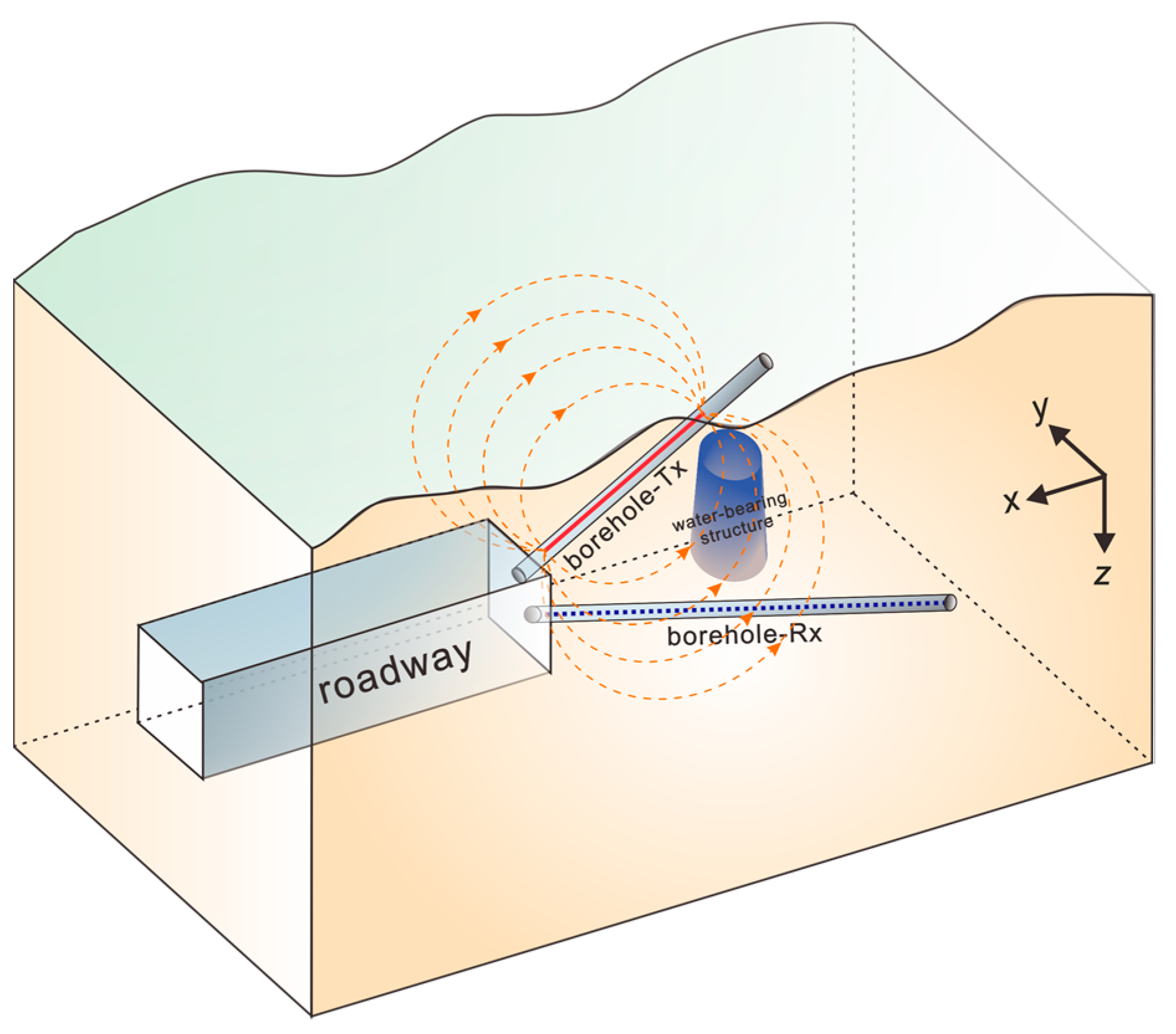
2. Cross-Hole Grounded-Wire-Source Transient Electromagnetic System

This paper introduces a novel transient electromagnetic (TEM) method utilizing a cross-hole grounded-wire source, as depicted in Figure 1. In this method, a grounded current supply conductor is placed in a borehole ahead of the working face. A step current is supplied through a connected transmitter, while a receiving probe is positioned in a borehole on the opposite side to perform point-by-point measurements. This configuration is designed to capture the distribution of the secondary electromagnetic field generated by induced eddy currents, enabling both the time and spatial signal observation of the geological target surrounding the borehole. The secondary field, which propagates through the rock mass with lower attenuation compared to air, produces higher signal amplitudes, leading to improved signal-to-noise ratios and lateral resolution. This results in the more effective detection of geological features. Furthermore, the grounded-wire-source configuration facilitates long-range, high-precision exploration. Depending on the number of boreholes in front of the working face, multiple survey lines and sources can be deployed [40]. This setup can generate a 3D observation pattern, which provides a theoretical foundation for subsequent 3D inversion. In practical engineering applications, following the completion of preliminary geophysical exploration, drilling verification is necessary. Hence, utilizing existing boreholes for our cross-hole method requires minimal additional investment. Moreover, this approach mitigates the limitation of relying on a single borehole, thereby providing more comprehensive data for advanced exploration.

3. Three-Dimensional Finite Element Method Forward Modeling Theory

3.1. Three-Dimensional Finite Element Method Algorithm

Boreholes in roadways are typically not arranged vertically but inclined at a certain angle relative to the working face. This configuration places higher demands on the forward modeling algorithms. The finite difference (FD) and integral equation (IE), which rely on structured grids, have limitations in accurately representing this inclined borehole model. As a result, the finite-element (FE) method using unstructured tetrahedral grids [41] is employed for modeling. In this approach, the computational domain Ω is initially divided into a finite number of tetrahedral meshes, as illustrated in Figure 2. The forward modeling of the cross-hole grounded-wire-source TEM is based on full-space theory, which simplifies the background model as it does not need to consider the influence of air.

Starting from Maxwell’s equations and using the Galerkin weighted residual method [42], the residual $R$ of the electric field diffusion equation can be expressed as

$$\begin{array}{l}{R}^e=\\ {{\displaystyle \iiint }}_{{\mathsf{\Omega }}^s}\mathbf{w}\cdot \left({\displaystyle \frac{1}{\mu }}\nabla \times \nabla \times \mathbf{E}\left(t\right)+\sigma {\displaystyle \frac{\partial \mathbf{E}\left(t\right)}{\partial t}}+{\displaystyle \frac{\partial j\left(t\right)}{\partial t}}\right)d\nu \end{array},$$

(1)

where $\mu$ and $\sigma$ are the magnetic and electric permeability, respectively, $E_{\left(t\right)}$ and $j_{\left(t\right)}$ are the electric field and current density at the time t, ${\mathsf{\Omega }}^e$ is the volume of the e-th element, and $w$ is the weight function. Furthermore, the interpolated basis function $N$ is the same as the weight function; Equation (1) can then be rewritten as

$$\begin{array}{l}{R}_i^e={\displaystyle \frac{1}{\mu }}{\displaystyle \sum }_{j=1}^6{E}_j^e\left(t\right){{\displaystyle \iint }}_{{\mathsf{\Omega }}^e}\nabla \times N_i\cdot \nabla \times N_{j}d\nu \\ +{\displaystyle \sum }_{j=1}^6{\displaystyle \frac{\partial E_j^e\left(t\right)}{\partial t}}{{\displaystyle \iiint }}_{{\mathsf{\Omega }}^e}{N}_i\sigma N_{j}d\nu +{{\displaystyle \iiint }}_{{\mathsf{\Omega }}^e}{N}_i\cdot {\displaystyle \frac{\partial j\left(t\right)}{\partial t}}d\nu \end{array},$$

(2)

The global system is constructed by assembling the elements in the computational domain with the weighted residuals $R=0$, so that Equation (2) can be expressed as a linear equation:

$$M{\displaystyle \frac{dE\left(t\right)}{dt}}+SE\left(t\right)+J=0,$$

(3)

where $M$ is the mass matrix, $S$ is the stiffness matrix, and $J$ is the source term matrix. The time derivative in Equation (3) is discretized by second-order backward Euler equation to obtain the following form:

$$\left(3M+2\mathsf{\Delta }tS\right)E^{i+2}=M\left(4E^{i+1}-E^i\right)-2\mathsf{\Delta }t{J}^{i+2},$$

(4)

where $E^{i+2}$, $E^{i+1}$, and $E^i$ denote the electric field at the (i + 2)-th, (i + 1)-th, and i-th moments, and $J^{i+2}$ is the source term at the (i + 2)-th moment. $\mathsf{\Delta }t$ denotes the time step, which is taken as a step growth in the calculations in this paper [43]. In this way, only Equation (4) needs to be solved to obtain the values of the electric field at all edges of the computational region and, thus, we can obtain the electromagnetic field parameters at the locations of the receivers. This leads to the following large linear equation:

$$KE=b,$$

(5)

The matrix form can be expressed as

$$\left(\begin{array}{cccccc}3M+2\mathsf{\Delta }{t}_{1}S& & & & & \\ -4M& 3M+2\mathsf{\Delta }{t}_{2}S& & & & \\ M& -4M& 3M+2\mathsf{\Delta }{t}_{3}S& & & \\ & M& -4M& 3M+2\mathsf{\Delta }{t}_{4}S& & \\ & & \ddots & \ddots & \ddots & \\ & & & M& -4M& 3M+2\mathsf{\Delta }{t}_{n}S\end{array}\right)\left(\begin{array}{c}{E}^1\\ E^2\\ E^3\\ E^4\\ ⋮\\ E^n\end{array}\right)=-\left(\begin{array}{c}2\Delta t_1{J}^1-3M{E}^0\\ 2\Delta t_2{J}^2+M{E}^0\\ 2\Delta t_3{J}^3\\ 2\Delta t_4{J}^4\\ ⋮\\ 2\Delta t_n{J}^n\end{array}\right),$$

(6)

Here, $n$ is the number of all discrete time steps. Subsequently, the Dirichlet boundary conditions are applied. The resulting electric field parameters for each moment are obtained by solving the linear Equation (6) with a direct solver [43]. The forward modeling programming in this paper was written in Fortran, which was executed with a personal workstation with a 3.20 GHz main frequency and 128 GB of RAM. In the numerical examples presented in this paper, a uniform grid refinement ratio of 1.4 was employed, with localized mesh refinement conducted at the receivers, sources, and boundary surfaces of the anomalous bodies.

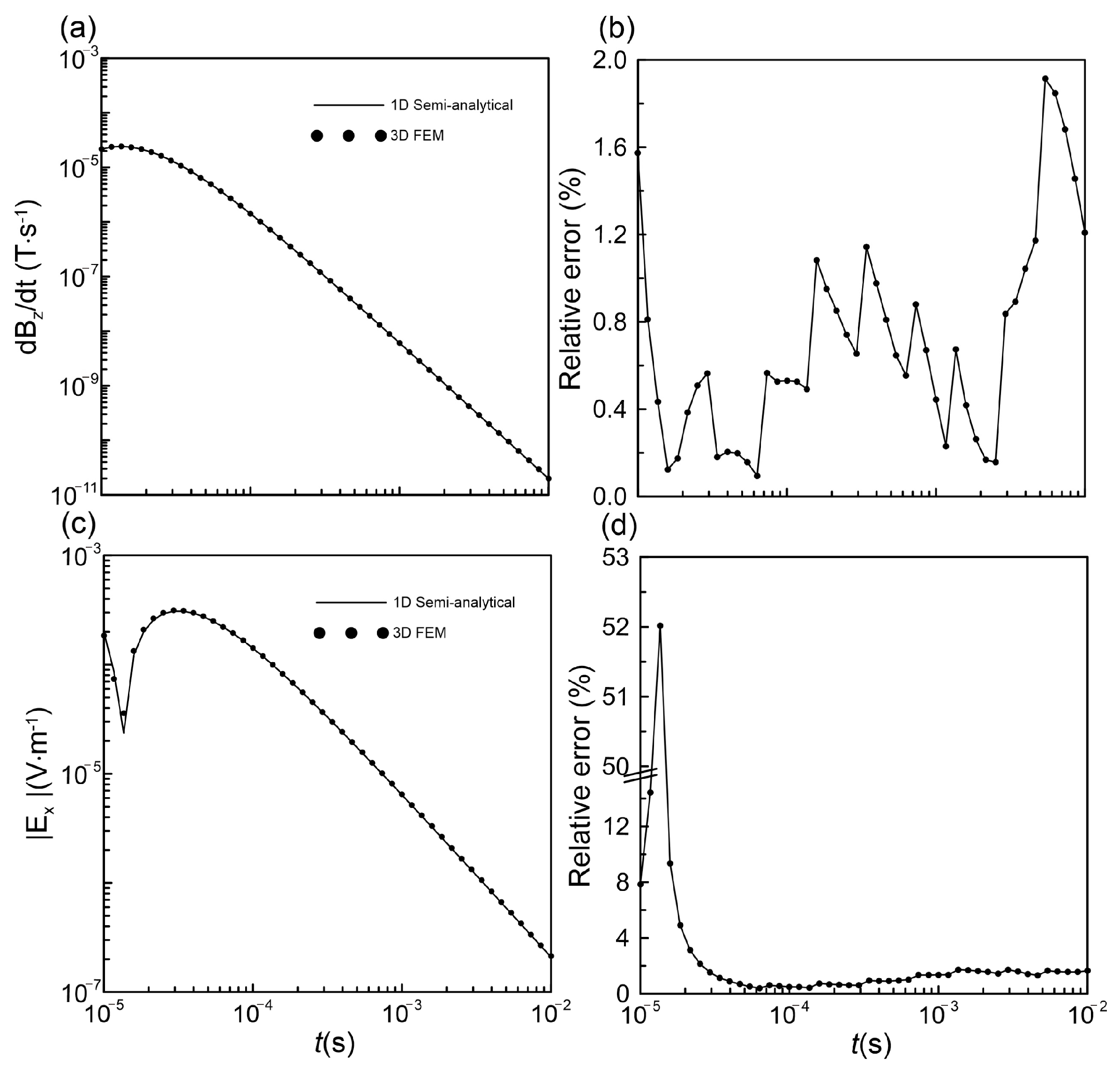
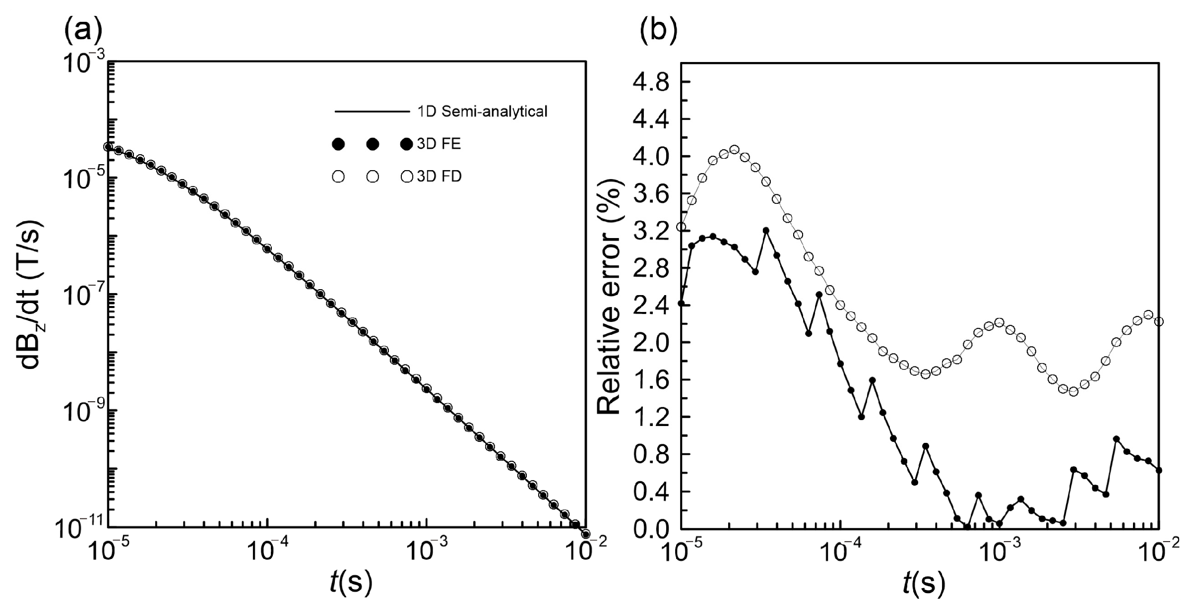
3.2. Validation Against Semi-Analytic Solution

In this paper, the semi-analytical solution of a 100 Ω·m full-space model was employed to verify the accuracy of our FE presented here. The transmitter consisted of a 100 m-long wire oriented along the x-direction, with the receivers positioned 100 m away from the source along its central axis. The forward modeling encompassed a total of 270,270 tetrahedral elements, comprising 316,559 edges, thereby defining a model with 316,559 degrees of freedom (DOFs). The extended boundary domain spanned 200 km × 200 km × 200 km in all three directions. The forward calculation involved 1100 time channels, increasing in a stepwise manner. For interpolation, 46 time channels between 10⁻⁵ s and 10⁻² s were selected to present the computed results of the electric field and induced electromotive force (EMF), which were then compared with 1D semi-analytical solutions for accuracy. The results are displayed in Figure 3. Both the electric field and EMF exhibited good agreement with the semi-analytical solutions. The relative errors for the EMF parameters were all below 2%. However, the electric field parameters exhibited a sign change between 0.1166 × 10⁻⁴ s and 0.1359 × 10⁻⁴ s, resulting in larger errors near the sign transition. Beyond 2.512 × 10⁻⁵ s, the relative errors also remained within 2%. It is evident that the FE presented in this paper demonstrated high numerical accuracy. To better illustrate the computational efficiency,

Table 1. Parameters for the full-space model using the FE method.

Elements	DOFs	Time Channel	Relative Error (%)	Time (s)	Max Memory (GB)
270,270	316,559	1100	0.70	550	41

lists the computational parameters for the EMF parameters, with all computation times and memory usage falling within reasonable limits. Thus, the results of the forward modeling study for the borehole TEM method using grounded-wire sources, conducted with the algorithms and codes presented in this paper, are reliable.

Taking the half-space model as an example, we considered a scenario where the resistivity of the air was 10⁻⁸ Ω·m and the background was 10⁻² Ω·m. We compared our results with those obtained using the established SLDMEM code using the finite-difference (FD) method, which was based on the work by Druskin and Knizhnerman [44] and was executed on servers. The results and parameters computed by the two algorithms are presented in Figure 4 and

Table 2. Parameters for the half-space model using the FE and FD methods.

Method	Elements	DOFs	Relative Error (%)	Time (s)
FE	363,546	424,425	1.31	770
SLDMEM	71 × 71 × 71	357,911	2.44	694

, respectively. It can be observed that the relative errors between the FE method presented in this paper and the semi-analytical solution for the half-space model were all below 3%, which were superior to those from the FD method. By further comparing the computational parameters of the two codes, we conclude that our FE code could achieve solutions with higher accuracy under similar numbers of DOFs while maintaining comparable computation times.

4. Results and Analysis of Three-Dimensional Forward Modeling

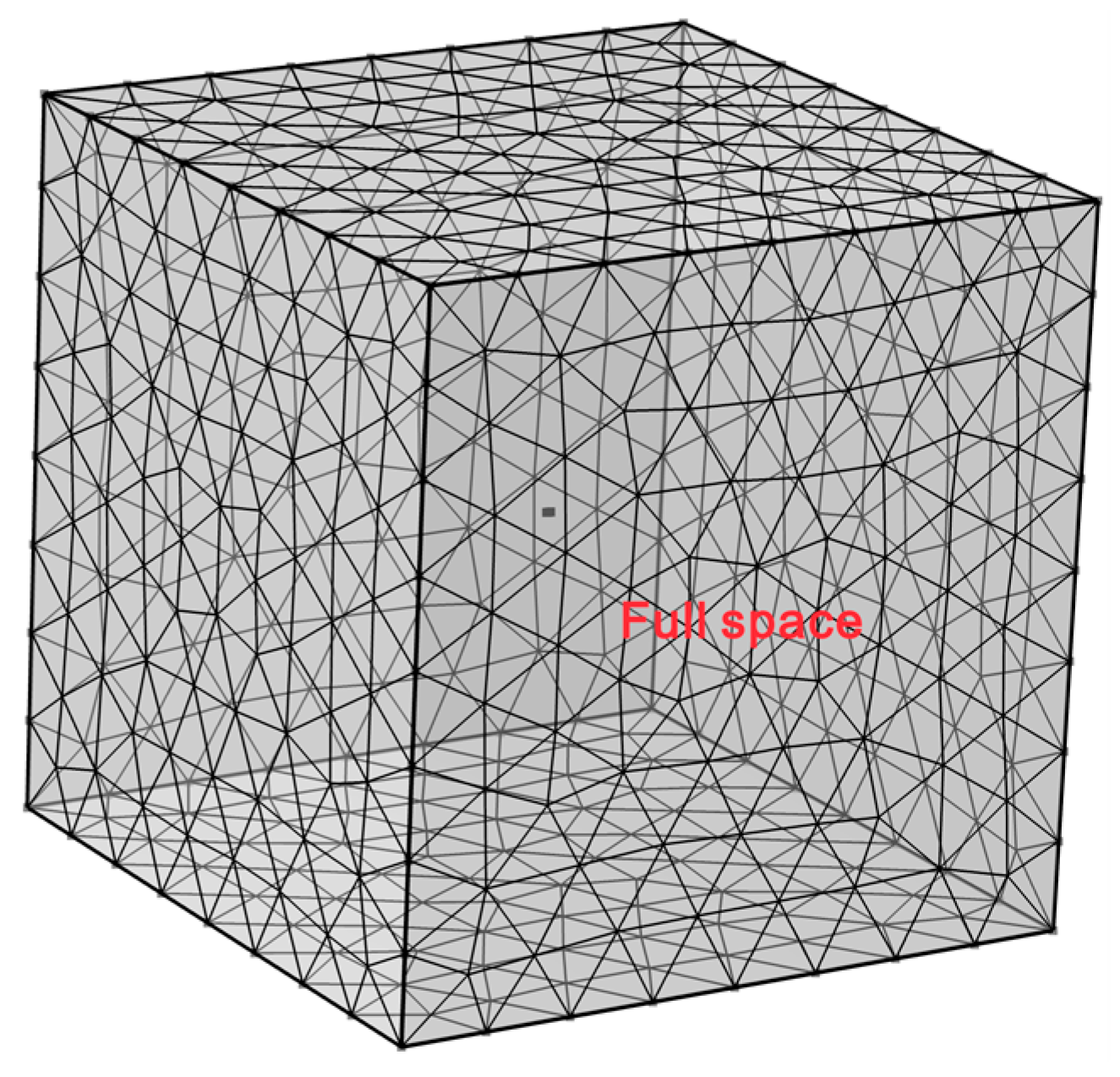
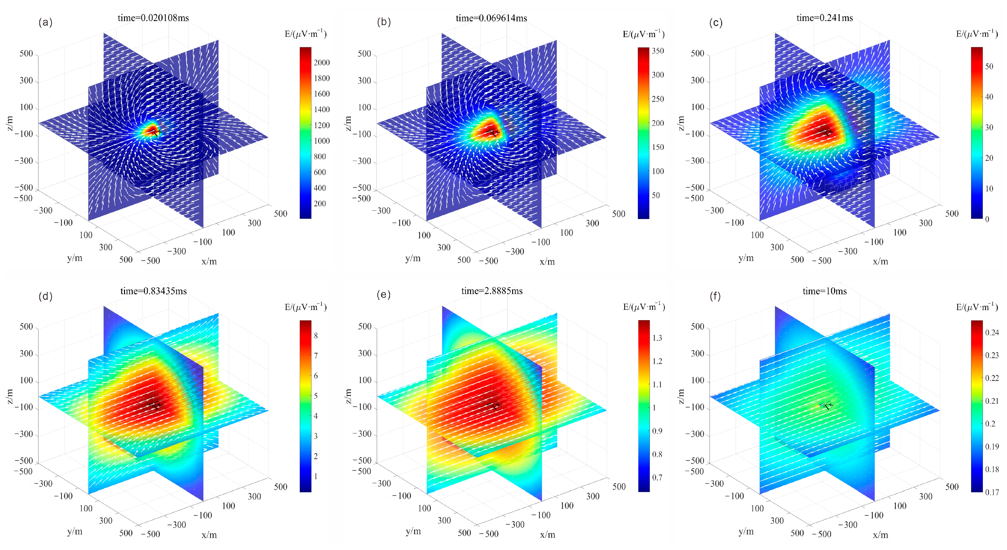
4.1. Full-Space Model

The cross-hole grounded-wire-source TEM model, employed for advanced exploration, is typically located at depths of up to 500 m below the surface, which can be approximated as a full-space environment. Consequently, this study modeled a 100 Ω·m full-space background, with the emitting source wires deployed along the x-direction, extending 100 m in length. Figure 5 illustrates the electric field diffusion, where the electric field components are represented by a color bar, with arrows indicating their directions. At early times, the electric field was stronger near the wire, originating from the positive terminal and returning to the negative terminal in a vortex-like pattern. As time progressed, the center of the electric field remained at the source, but its strength gradually diminished. Furthermore, the direction of the electric field evolved over time. At a later time, the x-component of the electric field near the source became the dominant component, while the y- and z-components approached zero. This indicates that the electric field diffusion was more prominently aligned with the wire direction. In the TEM geoelectric model of the cross-hole grounded-wire source, the borehole was not aligned with the model coordinate axes but was tilted at an angle. Therefore, the final forward modeling calculations required transforming the electric field components into the receiver’s directional coordinates.

4.2. Single-Anomaly Model

To evaluate the detection capability of the configuration shown in Figure 1, a 3D model was designed to analyze the response of anomalous bodies under various scenarios. After obtaining the receivers along the survey line, the boundaries of the anomalous bodies could be identified through differentiation, as expressed below:

$$E^{\prime }={\left[\begin{array}{cccc}{\displaystyle \frac{\partial E_1}{\partial r}}& {\displaystyle \frac{\partial E_2}{\partial r}}& \cdots & {\displaystyle \frac{\partial E_t}{\partial r}}\end{array}\right]}^{\prime },$$

(7)

Since it is difficult to observe a spatially continuous electric field in practice and only spatially discrete electric fields can be measured, the difference in Equation (7) is expressed in following matrix:

$${\mathit{E}}_{t\times \left(n-1\right)}^{\prime }={\displaystyle \frac{1}{\mathsf{\Delta }\mathrm{r}}}\left[\begin{array}{cccc}{E}_{11}& E_{12}& \cdots & E_{1n}\\ E_{21}& E_{22}& \cdots & E_{2n}\\ ⋮& ⋮& \ddots & ⋮\\ E_{t1}& E_{t2}& \cdots & E_{tn}\end{array}\right]{\left[\begin{array}{cccc}-1& & & \\ 1& -1& & \\ & 1& \ddots & \\ & & \ddots & -1\\ & & & 1\end{array}\right]}_{n\times \left(n-1\right)},$$

(8)

where r represents the direction vector of the survey line and $\mathsf{\Delta }\mathrm{r}$ is the distance between receivers, with $t$ and $n$ denoting the number of time moments and measuring electrodes. In this paper, we focus our attention on the EM response of the cross-hole grounded-wire-source TEM model. Taking multiple forward models as examples, we verified the effectiveness of this exploration method and assessed its sensitivity to parameters such as the size, resistivity contrast, and spatial location of the anomalous bodies.

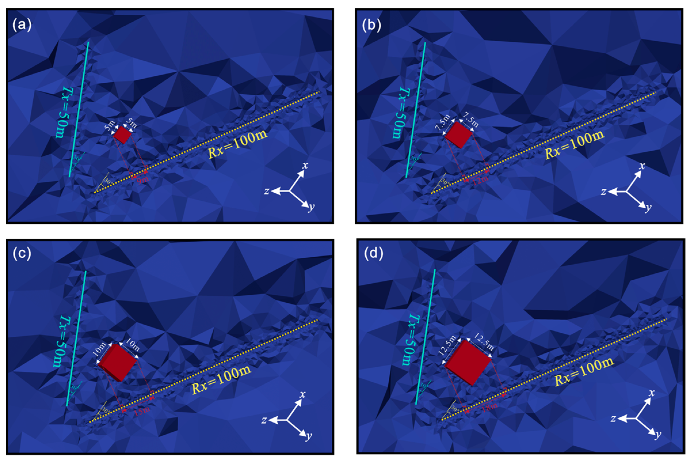
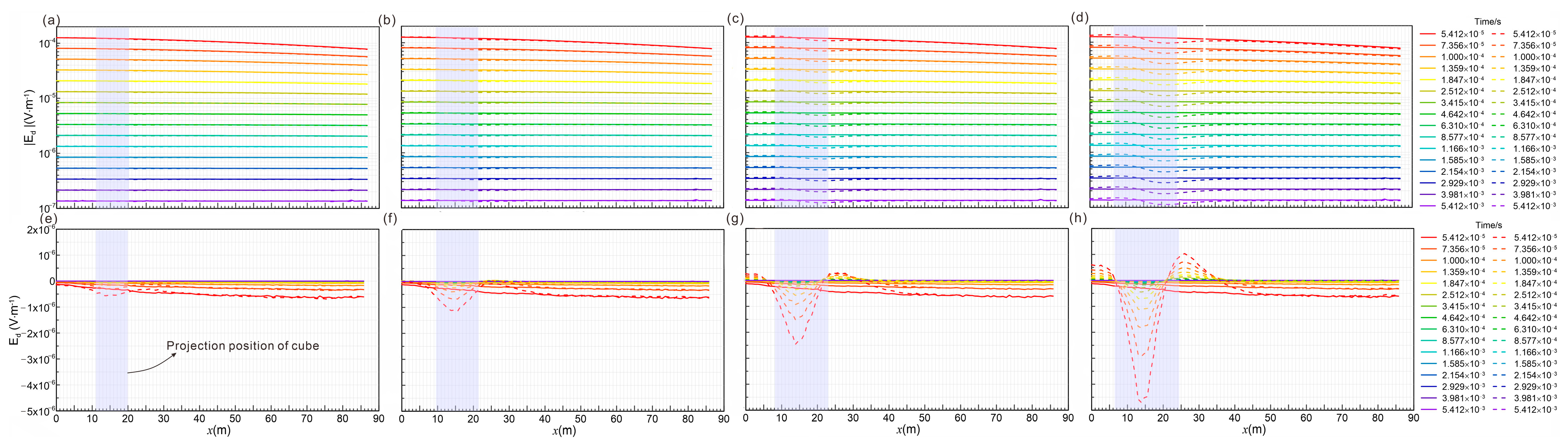
4.2.1. Individual Anomalies with Different Edge Lengths

To assess the feasibility of detecting anomalies using our cross-hole grounded-wire-source TEM method, four 10 Ω·m cubic anomaly models with a common central point, located between the transmitters and receivers, were designed. The side lengths of the cubes were 5 m, 7.5 m, 10 m, and 12.5 m, with a background resistivity of 100 Ω·m, as shown in Figure 6. In the z = 0 plane, two boreholes, zk1 and zk2, were positioned at angles of 30° and −30° along the y-axis. The grounded-wire source was placed in borehole zk1, with a length of 50 m, while the survey line was positioned in borehole zk2, with a 1 m spacing between measuring electrodes, resulting in a total of 101 points. The arrangement parameters were consistent with those used in the following models.

For the model described above, the EM forward modeling of our configuration was performed using the 3D FE algorithm, and the simulation results are presented in Figure 7. Figure 7a–d show the multi-channel electric field curves along the zk2 direction, where solid and dashed lines represent the full-space background model and the low-resistance anomaly model. The cubic anomalies are highlighted as purple blocks, corresponding to their projected locations along the survey line. When the cube’s volume was small (r = 5), the electric field curve closely matched the background. As the cube size increased (r = 7.5, 10 m, 12.5 m), the anomalies became more discernible, with the electric field exhibiting an “S”-shaped oscillation compared to the background. In Figure 7e–h, the solid and dashed lines represent the first-order differential results of the electric field for the full-space and low-resistance anomaly models. These differential results reveal a negative region at the anomaly positions and positive regions on either side when compared to the full-space model. The boundaries of the anomalous body are clearly defined by the positive and negative interfaces. As the cube volume increased, both the electric field response and the differential parameter showed larger value ranges, making the anomalies easier to detect. These results demonstrate that the cross-hole grounded-wire-source EM method was effective in detecting anomalies. Moreover, applying first-order differential processing to the electric field data enhanced anomaly detection sensitivity, allowing for the more precise identification of anomaly boundaries.

4.2.2. Individual Anomalies with Different Distances and Resistivities

The resistivity of the target anomaly body, such as water-bearing structures or air-filled goafs, typically varies. Therefore, target anomalies can be designed to be low-resistance or high-resistance. In this example, the resistivity of low-resistance anomalies was 10 Ω·m, and that of high-resistance anomalies was 1000 Ω·m, with the background resistivity set to 100 Ω·m. The anomalies were positioned at different locations along the centerline between the transmitters and receivers (Figure 8), and the relationship between the anomaly response and distance was investigated.

As shown in Figure 9a,b,e,f, the electric field responses were opposite for the locations of high- and low-resistance anomalies. The differential curves show a negative region for the high-resistance cube with positive regions on both sides and a narrower value range compared to for the low-resistance cube. Furthermore, it is evident from Figure 9 that both the electric field value range and the differential value range gradually decreased as the distance increased. At a distance of 50 m, the electric field closely matched the half-space model, but the difference curve still shows a noticeable disparity. At 75 m, the difference between the two models became minimal, indicating that the differential parameter was more sensitive to anomalies. Moreover, the regions of variation in the model’s electric field parameters and the differential boundaries corresponded well with the anomaly locations.

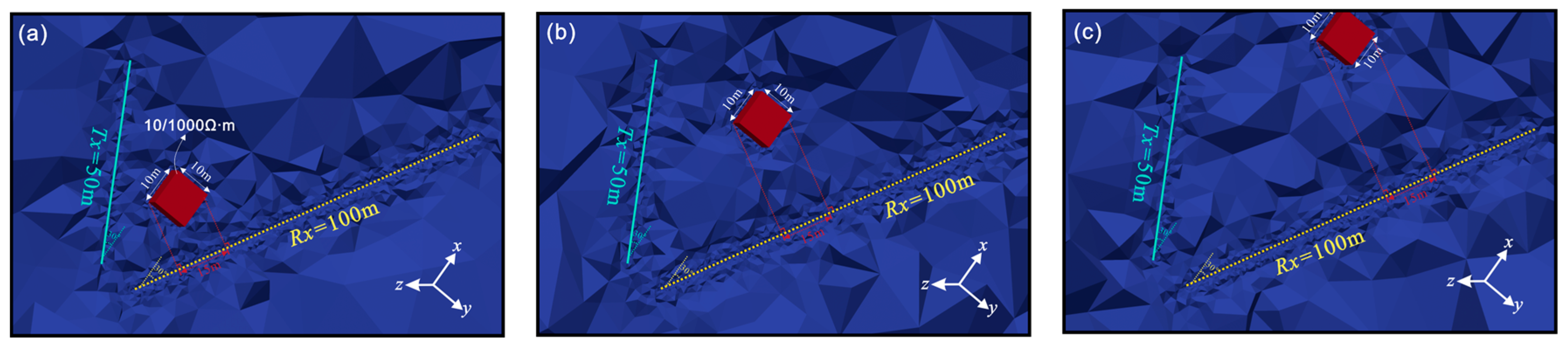
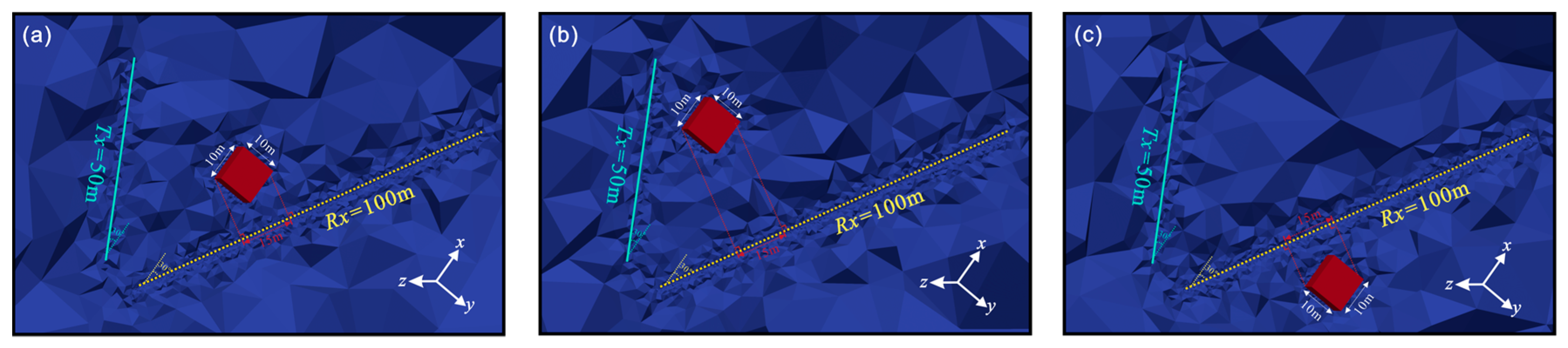
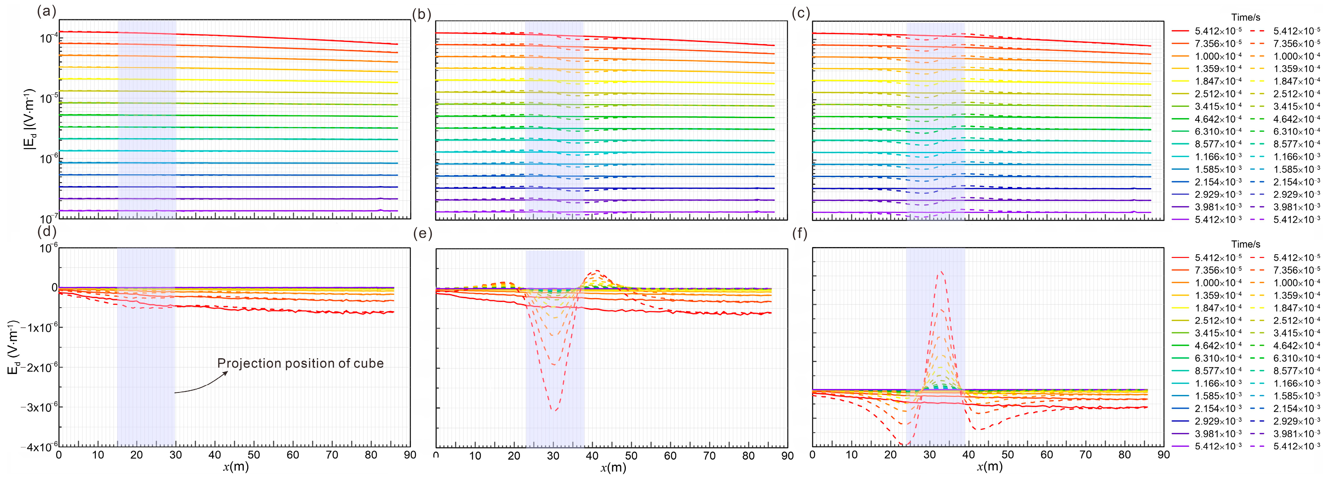
4.2.3. Individual Anomalies at Different Locations

This study also investigated models where the anomalous body was positioned at different locations. Specifically, the anomaly was placed near the grounded wire (Figure 10a), close to the survey line (Figure 10b), and outside the survey line (Figure 10c), with all other parameters consistent with those in Figure 6c. Figure 11 presents the forward modeling results for these scenarios. The anomaly near the transmitter showed a minimal response, making it more challenging to detect. In contrast, anomalies near the inner or outer areas of the survey line yielded larger and distinctly opposite responses. According to electromagnetic field diffusion theory, if the anomaly is near the source, the primary field arriving at the anomaly is stronger, inducing a stronger secondary field. However, since the anomaly was farther from the receivers, the received response was weaker due to attenuation. Conversely, when the anomaly was closer to the receivers, the primary field was weaker, but the secondary field underwent less attenuation, resulting in a stronger response. Additionally, when the anomalies were located on the outer side of the survey line, the electric field and first-order differential were opposite to those on the inner side, due to variations in the spatial distribution of the electric field.

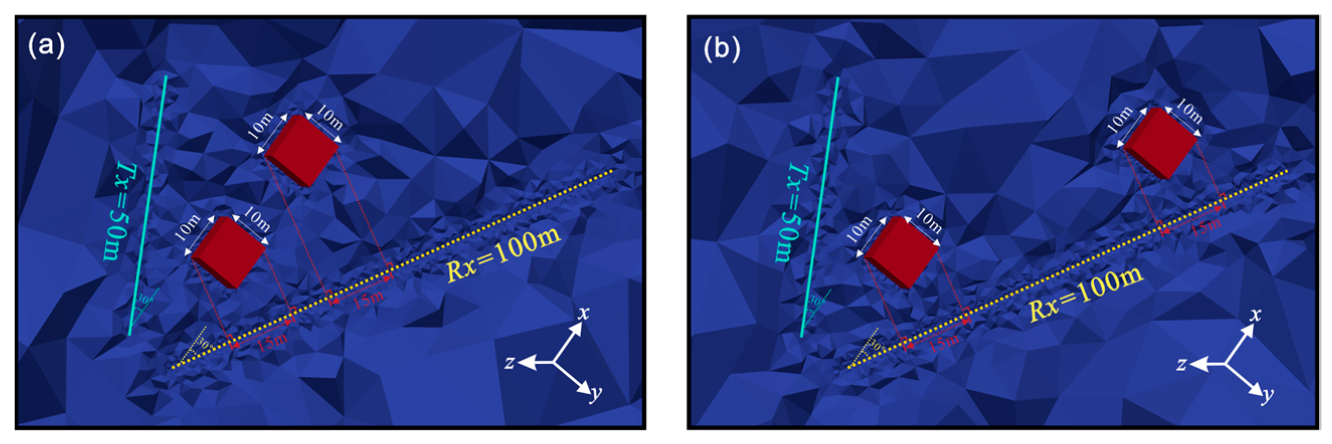
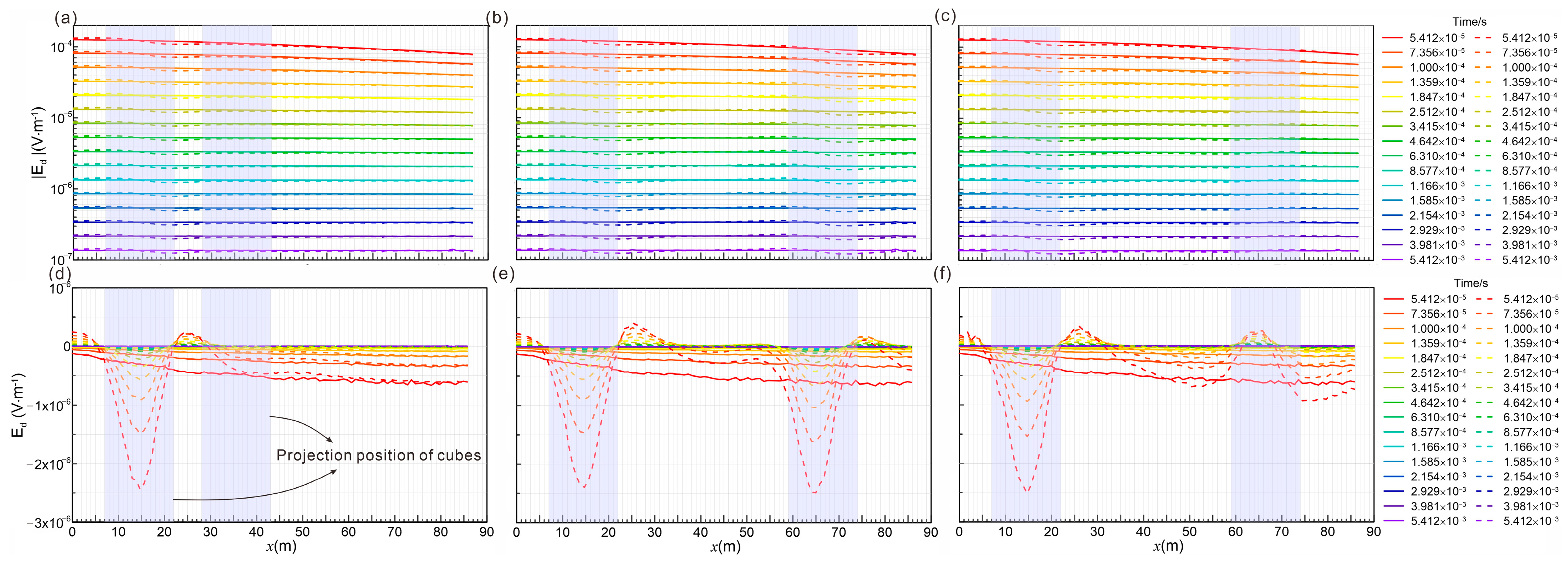
4.2.4. Two Anomalies’ Response and Localization

The previous calculations demonstrate the significant impact of the spatial positioning of anomalies on the electric field responses. In this section, we explore two scenarios involving two anomalies: (1) anomalies of 10 Ω·m positioned along the centerline between the grounded-wire source and the survey line (Figure 12a) and (2) anomalies located near the survey line (Figure 12b). For the latter configuration, two cases were considered: (a) both cubes had a resistivity of 10 Ω·m and (b) the left cube had a resistivity of 10 Ω·m while the right cube had a resistivity of 1000 Ω·m.

In Figure 13a, the anomaly on the left side is closer to both the transmitter and receiver, leading to a wider range and larger amplitude in the electric field. The proximity of the two anomalies causes the response from the right anomaly to be overshadowed by the left anomaly, making it nearly indistinguishable. In contrast, as shown in Figure 12b, both anomalies are positioned near the survey line but are farther apart. In the case where both anomalies are of low resistance (Figure 13b,e), or one anomaly is low-resistance and the other high-resistance (Figure 13c,f), the proposed configuration successfully distinguishes and identifies the anomalies. These results reinforce the importance of anomaly proximity to the survey line: the closer anomalies are to the survey line, the stronger their electric field responses. Therefore, maximizing the number of survey lines in our cross-hole exploration is essential to improve the detection and localization of surrounding anomalies.

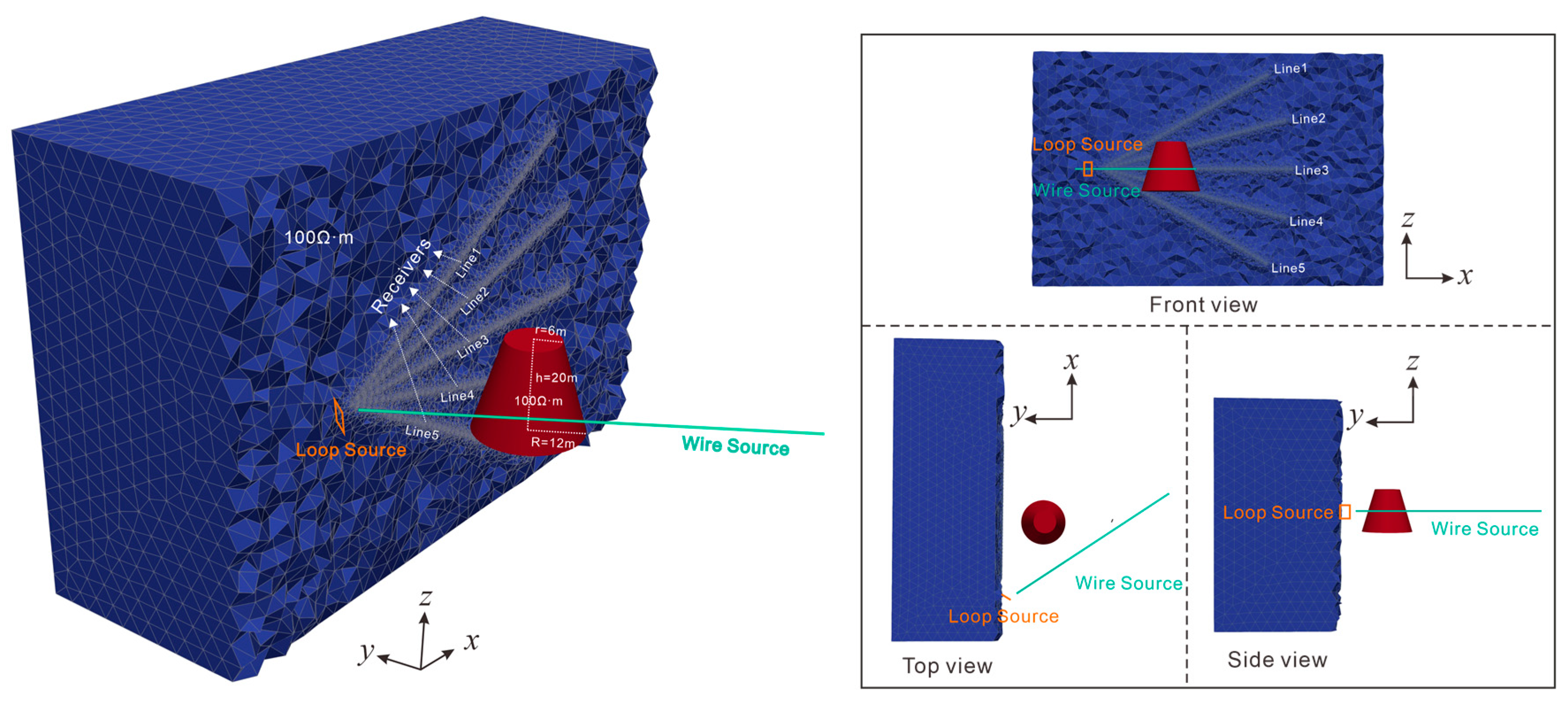
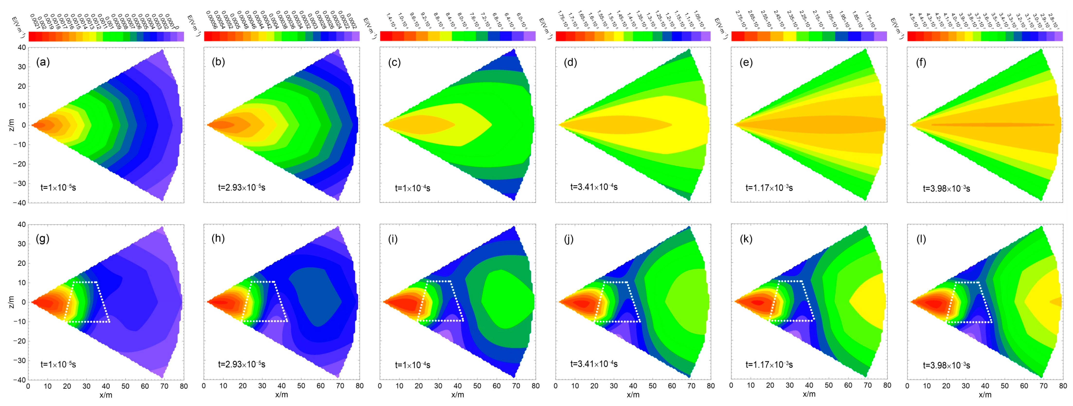
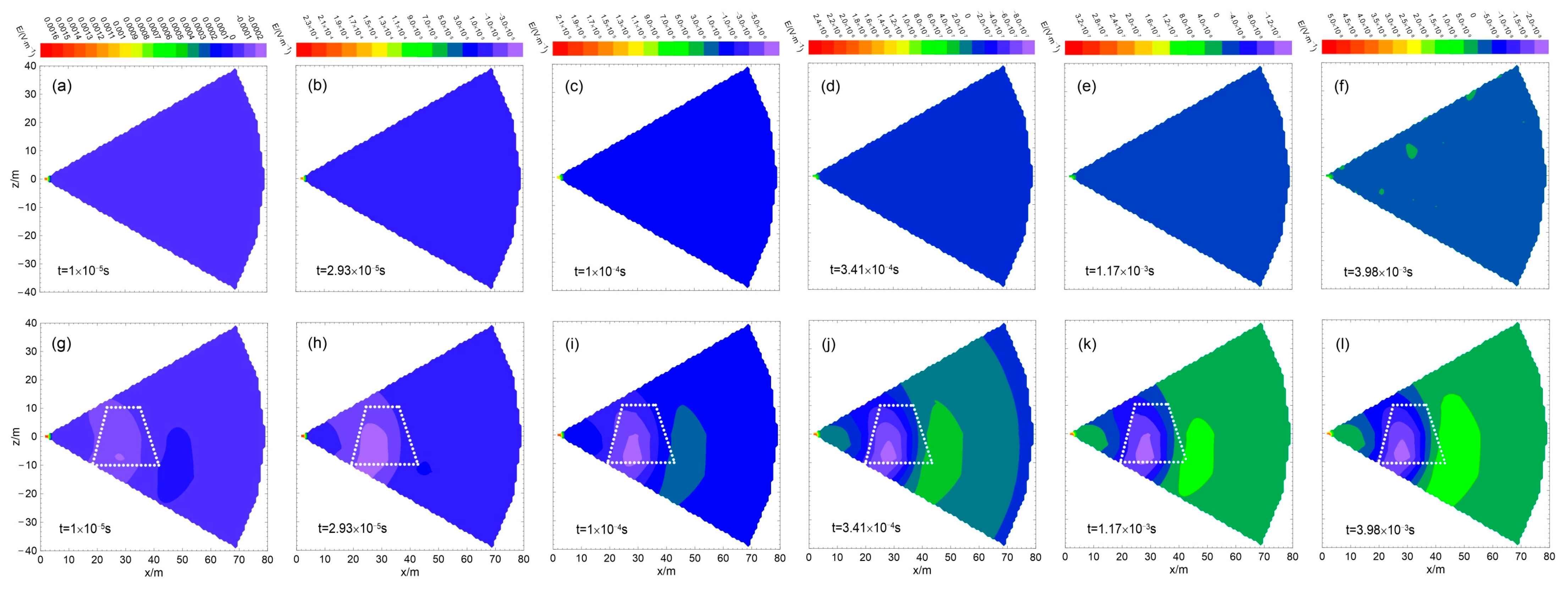
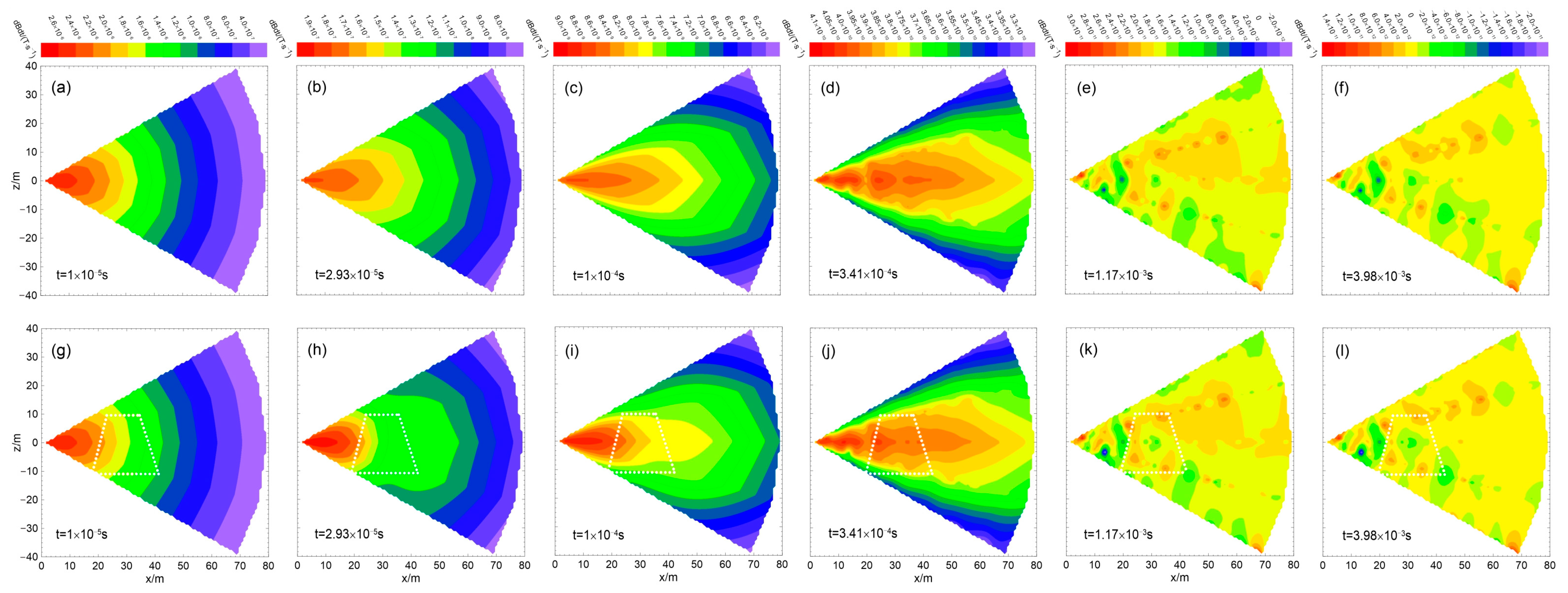
4.3. Detection of Water-Bearing Trap Columns by Cross-Hole EM with Multiple Grounded-Wire Source

In practical exploration, multiple boreholes are typically present within roadways. These boreholes can be used to deploy receivers for the 2D observation of anomalies, as illustrated in Figure 14. The survey consisted of five lines, arranged in a fan-shape within the x-z plane, with a 15° angular separation between adjacent lines. Each line had 41 electrodes, spaced 2 m apart. The grounded-wire source, 85 m in length, was positioned at a 60° angle to the survey plane. Between the grounded-wire source and the survey lines lay a dome-shaped trap column, with a resistivity of 1 Ω·m, a height of 20 m, and a top and bottom radius of 6 m and 12 m.

We present contour maps of the electric field responses for the five survey lines at different time steps, based on two models: the full-space model (Figure 15a–f) and the trap column model (Figure 15g–l). Both models share the same color bar for each time channel, with the locations of the trap columns indicated by white dashed lines. As the survey lines diverge from the grounded-wire source, the distance between them increases along the receiver coordinates. In the full-space model, the electric field decrease as the distance increases. However, in the trap column model, the presence of the water-bearing trap alters the electric field distribution, creating a low-value band in the trap column and generating high-value anomalies beyond the boundary. This effect becomes more pronounced over time, leading to a broader range of electric field response values.

Similarly, we performed differential calculations of the electric field in Figure 16. For the full-space model, the color bar has a broad range of values, resulting in differential results with minimal variation. In contrast, the electric field parameters from the trap column model more clearly delineate the location of the low-resistance anomaly, which appears as a negative center, with positive regions on either side. This differential analysis demonstrates that the anomaly boundary could be more precisely localized through first-order differential calculations.

In this study, comparisons with other configurations were also considered. However, due to the need to control for a single variable, direct comparisons between MTEM and STEM methods were not straightforward. To address this, we adopted the RBTEM method, which is based on boreholes. In this setup, the transmitting coil (orange line) was placed in the roadway, with a side length of 5 m, as shown in Figure 14. The measuring electrodes remained positioned in the borehole, and the location of the water-bearing trap column was consistent with that in the previous example. As a result, we obtained the contour maps of the EMF. Figure 17a–f display the responses for different time channels for the full-space model without anomalies, while Figure 17g–l show the responses of the water-bearing trap column. Notably, at middle times, the response values near the low-resistivity anomalous body decreased, indicating the presence of the water-bearing trap column. However, compared to the configuration proposed in this paper, it was more challenging to identify the boundaries of the anomalous body in this case. This was due to the inherently smaller EMF values observed and the weaker late-time signals. In contrast, the cross-hole grounded-wire-source configuration used in this paper produced stronger signals, allowing the anomalous body to be identified across almost all time channels.

4.4. Discussion

The case studies presented in this paper, based on 1D and 2D measurements, demonstrate that the proposed configuration effectively identified the characteristics of anomalous bodies. However, for more complex 3D observations, additional boreholes oriented in various directions were required to provide adequate support, which is a crucial consideration for future practical applications. With sufficient exploration data, more accurate 3D inversion becomes feasible. It is noteworthy that boreholes in roadways are often distributed in different directions and at varying depths, which can complicate the processing and interpretation of inversion. Nevertheless, since this exploration method improves detection accuracy, the ability to achieve 3D detection and inversion is expected to offer new opportunities for the precise exploration of underground spaces.

5. Conclusions

This paper addresses the challenges of severe interference and limited detection accuracy in advanced underground exploration by proposing an innovative cross-hole grounded-wire-source TEM. A detailed equipment arrangement scheme is presented, and the technique is validated using flexible unstructured FE methods for forward modeling. The following conclusions are drawn:

(1)

Larger volumes, lower resistivity values, and closer proximity of anomalous bodies result in larger response amplitudes, thereby improving detection effectiveness.

(2)

High-resistivity and low-resistivity anomalous bodies produce opposite anomalies (positive and negative, respectively) in the electric field. The system is more sensitive to low-resistivity anomalous bodies, making it particularly useful for detecting water-bearing targets in coal mines.

(3)

The position of the receivers has a greater impact on the final response strength than the source location. This suggests that the borehole-based arrangement proposed in this paper improves detectability.

(4)

The proposed setup can effectively determine key parameters, such as the anomalous body’s size, resistivity contrasts, and spatial position by analyzing changes in the electric field and first-order differential derivatives. This allows for the approximate localization of the anomaly’s boundary. Moreover, the cross-hole arrangement takes advantage of borehole spatial positioning, offering multi-directional information about the detected target.

(5)

In the collapse column model with multiple survey lines, both the electric field response and first-order differential results clearly delineate the boundary of the collapse column, demonstrating significantly improved detection accuracy over the traditional BRTEM method. Additionally, this configuration enables 2D/3D observations in roadway environments.

Overall, the cross-hole grounded-wire-source TEM proposed herein demonstrates excellent detection performance, particularly in water-bearing target exploration in underground spaces. This study introduces the technical concept of the method and establishes a theoretical foundation for future work, which will involve field data acquisition and validation.

References

1. Xue, G.Q.; Li, X.; Di, Q.Y. The progress of TEM in theory and application. Prog. Geophys. 2007, 22, 1195–1200. [Google Scholar]
2. Nabighian, M.N. Time-domain electromagnetic methods of exploration. Geophysics 1984, 49, 849–853. [Google Scholar] [CrossRef]
3. Sun, H.; Zhang, Y.; Zhao, Y.; Liu, Y. Present study situation review of borehole transient electromagnetic method. Coal Geol. Explor. 2022, 50, 85–97. [Google Scholar]
4. Xue, G.; Pan, D.; Yu, J. Review the applications of geophysical methods for mapping coal-mine voids. Prog. Geophys. 2018, 33, 2187–2192. [Google Scholar]
5. Cheng, J.; Li, F.; Peng, S.; Sun, X. Research and development direction on advanced detection in mine roadway working face using geophysical methods. J. China Coal Soc. 2014, 39, 1742–1750. [Google Scholar]
6. Yu, J.C. Exploration Prospecting for TEM in Mine; China University of Mining and Technology Press: Xuzhou, China, 2017. (In Chinese) [Google Scholar]
7. Jiang, Z.; Yue, J.; Liu, S. Mine transient electromagnetic observation system of small multi-turn coincident configuration. J. China Coal Soc. 2007, 32, 1152–1156. [Google Scholar]
8. Su, M.; Xia, T.; Xue, Y.; Mao, D.; Qiu, D.; Zhu, J.; Wang, P. Small fixed-loop transient electromagnetic in tunnel forward geological prediction. Geophys. Prospect. 2020, 68, 1399–1415. [Google Scholar] [CrossRef]
9. Chen, W.; Song, W.; Lei, K.; Zhu, Y. Application of surface-to-roadway TEMs for detecting deep aquifers in coal fields: An example from North China. J. Appl. Geophys. 2023, 219, 105242. [Google Scholar] [CrossRef]
10. Jiang, Z.; Liu, L.; Liu, S.; Yue, J. Surface-to-underground transient electromagnetic detection of water-bearing goaves. IEEE Trans. Geosci. Remote Sens. 2019, 57, 5303–5318. [Google Scholar] [CrossRef]
11. Yuan, L.; Zhang, P. Development status and prospect of geological guarantee technology for precise coalmining. J. China Coal Soc. 2019, 44, 2277–2284. [Google Scholar]
12. Spies, B. Electrical and electromagnetic borehole measurements: A review. Surv. Geophys. 1996, 174, 517–556. [Google Scholar] [CrossRef]
13. Cuevas, N.H. Insights on electromagnetic scattering by steel casings in surface-to-borehole and borehole-to-surface methods. Lead. Edge 2022, 41, 93–99. [Google Scholar] [CrossRef]
14. Castillo-Reyes, O.; Queralt, P.; Marcuello, A.; Ledo, J. Land CSEM simulations and experimental tests using metallic casing in geothermal exploration Vallès Basin (NE Spain) case study. IEEE Trans. Geosci. Remote Sens. 2022, 60, 1–13. [Google Scholar] [CrossRef]
15. Castillo-Reyes, O.; Queralt, P.; Pias-Varas, P.; Ledo, J.; Rojas, O. Electromagnetic subsurface imaging in the presence of metallic structures: A review of numerical strategies. Surv. Geophys. 2024, 45, 1–35. [Google Scholar] [CrossRef]
16. Cuevas, N.H. An approximate inversion scheme for surface-borehole electromagnetic in the presence of steel casing: 1D implementation. Geophysics 2021, 86, E111–E121. [Google Scholar] [CrossRef]
17. Cuevas, N.H. Insights on electromagnetic field distribution due to a vertical electric dipole source inside an infinite steel casing. Geophysics 2024, 89, E47–E59. [Google Scholar] [CrossRef]
18. Heagy, L.J.; Oldenburg, D.W. Impacts of magnetic permeability on electromagnetic data collected in settings with steel-cased wells. Geophys. J. Int. 2023, 234, 1092–1110. [Google Scholar] [CrossRef]
19. Heagy, L.J.; Oldenburg, D.W. Modeling electromagnetics on cylindrical meshes with applications to steel-cased wells. Comput. Geosci. 2019, 125, 115–130. [Google Scholar] [CrossRef]
20. Heagy, L.J.; Oldenburg, D.W. Electrical and electromagnetic responses over steel-cased wells. Lead. Edge 2022, 41, 83–92. [Google Scholar] [CrossRef]
21. Yang, H.; Yue, J.; Hu, W.; Li, F.; Liu, Z. The characteristics of the early signal in TEM affected by self-induction of multiturn coil. Comput. Tech. Geophys. Geochem. Explor. 2007, 29, 96–98. [Google Scholar]
22. West, R.C.; Ward, S.H. The borehole transient electromagnetic response of a three-dimensional fracture zone in a conductive half-space. Geophysics 1988, 53, 1469–1478. [Google Scholar] [CrossRef]
23. Paggi, J.; Macklin, D. Discovery of the Eureka volcanogenic massive sulphide lens using downhole electromagnetics. Explor. Geophys. 2016, 47, 248–257. [Google Scholar] [CrossRef]
24. Pardo, D.; Torres-Verdín, C.; Zhang, Z. Sensitivity study of borehole-to-surface and crosswell electromagnetic measurements acquired with energized steel casing to water displacement in hydrocarbon-bearing layers. Geophysics 2008, 73, F261–F268. [Google Scholar] [CrossRef]
25. Li, J.; He, Z.; Xu, Y. Three-dimensional numerical modeling of surface-to-borehole electromagnetic method for monitoring reservoir. Appl. Geophys. 2017, 14, 559–569. [Google Scholar]
26. Su, B.; Yu, J.; Królczyk, G.; Gardoni, P. Innovative Surface-Borehole Transient Electromagnetic Method for Sensing the Coal Seam Roof Grouting Effect. IEEE Trans. Geosci. Remote Sens. 2022, 60, 1–9. [Google Scholar] [CrossRef]
27. Li, K.; Sun, H.; Cheng, M.; Guo, J. CO2 injection monitoring using transient electromagnetic in ground-borehole configuration. J. Environ. Eng. Geophys. 2018, 23, 335–348. [Google Scholar] [CrossRef]
28. Cuevas, N.H.; Pezzoli, M. On the effect of the metal casing in surface-borehole electromagnetic methods. Geophysics 2018, 83, E173–E187. [Google Scholar] [CrossRef]
29. Wang, L.; Yin, C.; Liu, Y.; Su, Y.; Ren, X.; Hui, Z.; Zhang, B.; Xiong, B. Three-dimensional forward modeling for the SBTEM method using an unstructured finite-element method. Appl. Geophys. 2021, 18, 101–116. [Google Scholar]
30. Guo, Q.; Mao, Y.; Yan, L.; Chen, W.; Yang, J.; Xie, X.; Zhou, L.; Li, H. Key Technologies for Surface-Borehole Transient Electromagnetic Systems and Applications. Minerals 2024, 14, 793. [Google Scholar] [CrossRef]
31. Chen, W.; Han, S.; Khan, M.Y.; Chen, W.; He, Y.; Zhang, L.; Hou, D.; Xue, G. A surface-to-borehole TEM system based on grounded-wire sources: Synthetic modeling and data inversion. Pure Appl. Geophys. 2020, 177, 4207–4216. [Google Scholar] [CrossRef]
32. Wang, L.; Liu, Y.; Yin, C.; Su, Y.; Ren, X.; Zhang, B. Three-Dimensional Dual-Mesh Inversions for Sparse Surface-to-Borehole TEM Data. Remote Sens. 2023, 15, 1845. [Google Scholar] [CrossRef]
33. Krivochieva, S.; Chouteau, M. Whole-space modeling of a layered earth in time-domain electromagnetic measurements. J. Appl. Geophys. 2002, 50, 375–391. [Google Scholar] [CrossRef]
34. Fan, T. Experimental study on the exploration of coal mine goaf by dynamic source and fixed reception roadway-borehole TEM detection method. J. China Coal Soc. 2017, 42, 3229–3238. [Google Scholar]
35. Fan, T.; Li, P.; Qi, Z.; Zhao, Z.; Fang, X.; Yan, B.; Zhao, R.; Liu, L.; Li, Y.; Fang, Z. Borehole transient electromagnetic stereo imaging method based on horizontal component anomaly feature clustering. J. Appl. Geophys. 2022, 197, 104537. [Google Scholar] [CrossRef]
36. Li, X.; Han, D.; Wang, C.; Fan, T.; Li, B. Application of roadway-borehole TEM in water-bearing and water conducting structure prospecting. Coal Geo. China 2019, 31, 77–82. [Google Scholar]
37. Sun, Q.; Ding, H.; Sun, Y.; Yi, X. Borehole transient electromagnetic response calculation and experimental study in coal mine tunnels. Meas. Sci. Technol. 2024, 35, 045112. [Google Scholar] [CrossRef]
38. Li, H.; Li, X.; Qi, Z.; Cao, K. Seismic prediction of unfavorable geobodies in tunnels using the borehole-roadway transient electromagnetic method. Geophys. Geochem. Explor. 2024, 48, 1215–1222. [Google Scholar]
39. Chen, D.; Cheng, J.; Wang, A. Numerical simulation of drillhole transient electromagnetic response in mine roadway whole space using integral equation method. Chinese J. Geophys. 2018, 61, 4182–4193. [Google Scholar]
40. Li, X.; Hu, W.; Xue, G. 3D modeling of multi-radiation source semi-airborne transient electromagnetic response. Chinese J. Geophys. 2021, 64, 716–723. [Google Scholar]
41. Qiu, C.; Güttel, S.; Ren, X.; Yin, C.; Liu, Y.; Zhang, B.; Egbert, G. A block rational Krylov method for 3-D time-domain marine controlled-source electromagnetic modelling. Geophys. J. Int. 2019, 218, 100–113. [Google Scholar] [CrossRef]
42. Li, J.; Lu, X.; Farquharson, C.; Hu, X. A finite-element time-domain forward solver for electromagnetic methods with complex-shaped loop sources. Geophysics 2018, 83, E117–E132. [Google Scholar] [CrossRef]
43. Yin, C.; Qi, Y.; Liu, Y. 3D time-domain airborne EM forward modeling with topography. J. Appl. Geophys. 2016, 134, 11–22. [Google Scholar] [CrossRef]
44. Druskin, V.; Knizhnerman, L. Spectral approach to solving three dimensional Maxwell’s diffusion equations in the time and frequency domains. Radio Sci. 1994, 29, 937–953. [Google Scholar] [CrossRef]
Figure 1. Schematic diagram of cross-hole grounded-wire-source transient electromagnetic method.
Applsci 15 02672 g001
Figure 2. Grid subdivision for full-space EM model.
Applsci 15 02672 g002
Figure 3. The forward modeling responses of the full-space model along with the relative errors compared to the 1D semi-analytical solution, where (a,b) are the results for the induced electromotive force (EMF), while (c,d) are those of the electric field.
Applsci 15 02672 g003
Figure 4. A comparison between the results obtained using our FE and FD methods for a half-space model. Specifically, (a) shows the EMF parameters, while (b) displays the relative errors compared to the 1D semi-analytical solution.
Applsci 15 02672 g004
Figure 5. Diffusion of electric field response of grounded-wire-source EM method for full space model for time channel of (a) 0.020108 ms; (b) 0.069614 ms; (c) 0.241 ms; (d) 0.83435 ms; (e) 2.8885 ms; and (f) 10 ms.
Applsci 15 02672 g005
Figure 6. The forward modeling grid for a single cube with side lengths of (a) 5 m; (b) 7.5 m; (c) 10 m; and (d) 12.5 m.
Applsci 15 02672 g006
Figure 7. Multi-channel electric field and differential curves for cubes with (a,e) 5 m side length; (b,f) 7.5 m side length; (c,g) 10 m side length; and (d,h) 12.5 m side length.
Applsci 15 02672 g007
Figure 8. Cubic anomalies located at (a) 25 m (resistivity of 10 Ω·m or 1000 Ω·m), (b) 50 m, and (c) 75 m in the midline of the transmitters and receivers.
Applsci 15 02672 g008
Figure 9. Multi-channel electric field curves and differential curves for cube located at (a,e) 25 m (resistivity of 10 Ω·m), (b,f) 25 m (resistivity of 1000 Ω·m), (c,g) 50 m, and (d,h) 75 m in the midline of the transmitters and receivers.
Applsci 15 02672 g009
Figure 10. The cubes (a) close to the transmitters; (b) on the inner side and close to the survey line; and (c) on the outer side and close to the survey line.
Applsci 15 02672 g010
Figure 11. Multi-channel and difference curves for cubic anomalies (a,d) close to the transmitters; (b,e) on the inner side and close to the survey line; and (c,f) on outer side and close to the survey line.
Applsci 15 02672 g011
Figure 12. The positioning of the two anomalies (a) along the centerline between the grounded-wire source and the survey line and (b) near the survey line.
Applsci 15 02672 g012
Figure 13. Multi-channel electric field and differential curves for two cubic anomalies: (a,d) aligned along the centerline between the grounded-wire source and survey line; (b,e) located near the survey line with both anomalies of low resistance; (c,f) located near the survey line with one anomaly of low resistance and the other of high resistance.
Applsci 15 02672 g013
Figure 14. Model of water-bearing trap column and three-view drawing.
Applsci 15 02672 g014
Figure 15. Contour plots of electric field obtained by (af) full-space model and (gl) water-bearing trap column model.
Applsci 15 02672 g015
Figure 16. Contour plots of first-order difference in electric field obtained by (af) full-space model and (gl) water-bearing trap column model.
Applsci 15 02672 g016
Figure 17. Contour plots of EMF obtained by (af) full-space model and (gl) water-bearing trap column model.
Applsci 15 02672 g017