Intelligent Scheduling of a Pulsating Assembly Flow Shop Considering a Multifunctional Automated Guided Vehicle

Abstract

The pulsating assembly line is widely used in modern manufacturing, particularly in high-precision industries such as aerospace, where it greatly enhances production efficiency. To achieve overall optimization, both product scheduling and Automated Guided Vehicle (AGV) scheduling must be simultaneously optimized. However, existing research predominantly focuses on product scheduling, with limited attention given to AGV scheduling. This paper proposes an optimized solution for the pulsating assembly line scheduling problem, incorporating multifunctional AGV scheduling. A mathematical model is developed and three AGV selection strategies and three AGV standby strategies are designed to optimize AGV scheduling and control. To improve scheduling efficiency, nine heuristic strategies are introduced, along with the Variable Neighborhood Descent (VND) algorithm as a metaheuristic method for product scheduling. The VND algorithm refines the solution through multiple neighborhood searches, enhancing both the precision and efficiency of product scheduling. Our experimental results demonstrate that the proposed strategies significantly improve the production efficiency of pulsating assembly workshops, reduce AGV scheduling costs, and optimize overall production workflows. This study offers novel methods for intelligent scheduling in pulsating assembly workshops, contributing to the advancement of manufacturing toward “multiple varieties, small batches, and customization”.

1. Introduction

In recent years, advances in science and technology have increasingly shifted the manufacturing industry toward ‘multiple varieties, small batches, and customization’ [1]. Enterprises need to enhance production efficiency to reduce costs effectively. Zhang et al. developed an intelligent scheduling framework addressing complex issues such as optimizing lock progress, ship entry times, and ship positioning within lock cabins [2]. Momenikorbekandi et al. introduced a reinforcement learning (RL) model to improve scheduling performance in flexible job shop problems (FJSPs) [3]. Xu et al. proposed a deep reinforcement learning-based scheduling method to address workshop production challenges posed by crane complexity and dynamics [4]. Leyva-Pupo et al. proposed an intelligent scheduling reconfiguration (ISR) method leveraging machine learning to automate reconfiguration processes [5]. Zhao et al. developed an AGV scheduling application utilizing the Spring framework [6]. Jin et al. designed a model-free, end-to-end scheduling agent capable of interacting with cloud environments, outputting virtual machine task details, and handling cloud platform tasks [7]. Zhang et al. implemented an intelligent scheduling model and optimization algorithm in mining operations, achieving autonomous vehicle path planning [8]. Ibhaze et al. proposed an intelligent scheduling system. By using the DSSM algorithm [9]. Yang et al. developed an intelligent model for engine manufacturing and scheduling [10]. Shi et al. introduced deep reinforcement learning to schedule automated production lines, avoiding manual feature extraction and overcoming the lack of structured data sets [11]. Liu et al. developed an intelligent job scheduling method that can quickly and effectively generate process plans by combining the advantages of digital twins and hypernetworks [12]. Li et al. proposed a bulk cargo loading scheduling efficiency optimization method based on deep reinforcement learning [13]. Zou et al. proposed an intelligent scheduling method for the energy-saving operation of multiple trains based on a genetic algorithm and regenerative kinetic energy [14].

The pulsating assembly flow shop represents a significant approach to enhancing assembly efficiency in modern manufacturing. It is characterized by advanced industrialization, robust production rhythms, and high levels of digitization. This method is widely utilized in modern manufacturing, particularly within the aerospace industry. In 2000, Boeing pioneered the first pulsating assembly line, employing it for the production of Apache helicopters. The workflow of a pulsating assembly flow shop, illustrated in Figure 1, encompasses several stages. These stages include preliminary preparation, pulsation assembly line design, and continuous improvement [15].

The scheduling problem for pulsating assembly flow shops is a critical aspect of production planning. However, in practical scenarios, the complexity of assembly and resource constraints often result in assembly line imbalances. Assembly line balancing represents a typical NP-combinatorial optimization problem. This challenge has been extensively studied by researchers. Corominas et al. developed a mixed-integer linear programming method to enhance class E assembly line efficiency by optimizing station numbers and cycle times [16]. Similarly, Sikora et al. investigated welding process assembly lines, addressing multiple identical tasks in simple assembly line balancing problems through a mixed-integer linear programming model and branch-and-bound approach [17]. Zou et al. studied the multi-AGV scheduling problem with unloading safety detection in a matrix manufacturing workshop [18]. Li et al. proposed an indoor AGV positioning method combining vision and ultra wideband [19]. Wu et al. designed an intelligent manufacturing assembly line layout optimization model considering AGV path planning [20]. Lou et al. proposed the digital-twin-driven AGV scheduling and routing framework, aiming to deal with uncertainties in ACT [21].

The large volume of parts in pulsating assembly flow shops necessitates the use of AGVs for distribution. To reduce the number of required AGVs, multi-functional AGVs are employed, enabling each AGV to transport a variety of products. Efficient AGV scheduling is thus critical in pulsating assembly flow shops, playing a pivotal role in the production process and demanding careful attention. However, existing research on pulsating assembly flow shop scheduling primarily focuses on production scheduling, with limited attention given to AGV scheduling.

For example, Liang et al. proposed a three-stage integrated scheduling algorithm for AGV routing planning [22]. Meng et al. designed a belt-guided AGV car with a lifting module according to the design requirements of the production line of a drip irrigation belt rolling AGV car, which improved the production efficiency of the drip irrigation belt [23]. Vancea et al. developed an independent AGV that can operate autonomously and make decisions based on changes in the environment [24]. Popper et al. proposed a reinforcement learning multi-agent system for job scheduling and vehicle planning to optimize FJSP, such as AGV coordination [25]. Wang et al. developed a set of AGV scheduling system architectures based on the already successfully developed outdoor heavy AGV [26].

Addressing the research gap identified above, this paper explores the pulsating assembly flow shop scheduling problem with multifunctional AGVs (PAFSP_AGV). To tackle this issue, a mathematical model is established. We propose three AGV selection strategies and three AGV standby strategies. Additionally, three metaheuristic algorithms are introduced to solve the problem. Finally, the effectiveness of the AGV scheduling strategy and algorithms is validated through test cases.

The contributions of this paper are as follows:

(1) We proposed the architecture for solving the studied PAFSP_AGV problem and modeled the problem by establishing MILP models.

(2) We designed four AGV selection strategies and three AGV standby strategies for the studied PAFSP_AGV by considering specific problem characteristics.

(3) We proposed a heuristic algorithm and three meta-heuristics to solve the studied PAFSP_AGV to provide scheduling schemes under different computing times.

The remainder of this paper is organized as follows. Section 2 describes and models the problem under study. In Section 3, the AGV scheduling strategies are designed. Section 4 introduces the heuristic algorithms. Section 5 presents the metaheuristic algorithms. In Section 6, the experimental results are analyzed and discussed. Finally, Section 7 concludes the paper and outlines future work.

2. Materials and Methods

2.1. The AGV Scheduling Problem in the Pulsating Assembly Flow Shop

In the flow job shop scheduling problem, the processing system consists of machine tools with various functions. Each workpiece involves multiple processes. Each process is assigned to a specific machine tool, with identical processing routes for all workpieces. There is a sequential constraint between the processes of each workpiece. The flow shop scheduling problem is typically described as n jobs, each with m processes to be processed on m machines, where each process must be assigned to a different machine, and the processing order is identical for all jobs. The objective is to determine the processing sequence and start time for each workpiece on the machines to optimize a specific performance index (Figure 2).

In the PAFSP_AGV, it is assumed that n jobs, each consisting of m processes, are processed on m machines, with AGVs available in the workshop. Each process must be assigned to a distinct machine. The processing order is identical across all jobs, and AGVs are tasked with transporting each job. Each AGV can transport one job at a time, and only one AGV can be stationed near each machine. Before each process begins, the AGV must travel from the standby position to the pickup location and then transport the workpiece to the delivery position before the machine starts. The objective is to determine the processing sequence and start times for each workpiece on each machine to optimize a specific performance index.

At the start of production, all workpieces are stored in the Warehouse Management System (WMS), and all AGVs are docked in the charging room. The first workpiece to be processed is selected from the processing sequence, and the AGV scheduling system assigns an AGV to perform the task according to the selected strategy. The scheduling task is divided into three stages as follows. First, the AGV moves from the standby position to the workpiece pick-up location, from the charging room to the WMS; second, the AGV transports the workpiece from the pick-up location to the delivery position, moving from the WMS to the first processing machine of the first workpiece; finally, the AGV selects a docking position based on the scheduling strategy. Once the processing machine receives the workpiece, it begins the processing task. Once processing is complete, the call operation begins. The AGV scheduling system then performs the next task based on the call operation. This continues until all processes for all workpieces are completed and transported to the finished product buffer (BF).

2.2. Mathematical Model

Symbolic notes:

j: Job index, 1 ≤ j ≤ n.

i: Processing machine index, 1 ≤ I ≤ m.

k: AGV vehicle index, 1 ≤ k ≤ a.

h: AGV docking position index, 1 ≤ h ≤ b.

$u^v$: The cost of each AGV.

$u^d$: Unit distance cost of travel distance.

$n^c$: Number of charging piles.

n: Number of jobs.

m: Number of processing machines.

a: The number of AGVs.

b: The number of AGV stops.

$n^{wms}$: Number of three-dimensional garage parking spaces.

$n^{bf}$: Number of parking spaces in the finished product cache area.

$n^m$: Number of parking spaces per processing machine.

$\alpha$: Unit tardiness penalty.

N = {1,2,…,n }: The set of jobs.

M = {1,2,…,m }: The set of processing machines.

A = {1,2,…,a }: AGV set.

Parameters

$t_{j i}^p$: The processing time of workpiece j on machine i.

$t_{h1 h2}^m$: Transport time of vehicles between stops.

Decision variables:

$t_{j i}^C$: The completion time of job j on machine i.

$t_{n m}^C$: The completion time of the last process of the last job.

$x_{ijk}$: If AGV k transports workpiece i to machine j, then $x_{ijk}=1$; otherwise $x_{ijk}=0$.

$s_{s l}^k$: The moving distance of AGV k from the standby position to the pickup position.

$s_{l u}^k$: The moving distance of AGV k from the pickup position to the delivery position.

$s_{u s}^k$: The moving distance of AGV k from the delivery position to the standby position.

$t_{s l}^k$: The movement time of AGV k from the standby position to the pickup position.

$t_{l u}^k$: The movement time of AGV k from the pickup position to the delivery position.

$t_{u s}^k$: The movement time of AGV k from the delivery position to the standby position

${\pi }_{now}$: AGV current position sequence.

${\pi }_{target}$: AGV target position sequence.

${\pi }_{standby}$: AGV is currently in a standby state sequence.

Objective function:

$$minF\left(i,j,a\right)=\alpha \times t_{n m}^C+\sum _{j=1}^n\sum _{i=1}^m\sum _{k=1}^a{x}_{ijk}\times u^d\times \left(s_{s l}^k+s_{l u}^k+s_{u s}^k\right)+a\times u^v$$

(1)

The objective function of the PAFSP_AGV problem is given by Equation (1), which minimizes the sum of production delay cost, AGV transportation cost, and AGV usage cost.

Constraint conditions:

$$\sum _{j=1}^n\sum _{k=1}^a{x}_{ijk}=\mathrm{n},\forall i\in M$$

(2)

The transportation of all workpieces by AGVs to each processing machine is ensured by Equation (2).

$$\sum _{i=1}^m\sum _{k=1}^a{x}_{ijk}=\mathrm{m},\forall j\in N$$

(3)

The constraint in Equation (3) ensures that each workpiece is moved by AGVs to all processing machines.

$$\sum _{j=1}^n\sum _{i=1}^m{x}_{ijk}\ge 1,\forall k\in A$$

(4)

The constraint in Equation (4) ensures that each AGV participates in processing and transportation.

$$t_{j i}^C\ge max\left\{t_{j-1 i}^C+t_{j i-1}^C\right\}+t_{s l}^k+t_{l u}^k+t_{j i}^p$$

(5)

The constraint in Equation (5) limits the completion time of job j on machine i.

$$b=n^c+n^{wms}+n^{bf}+n^m$$

(6)

The constraint in Equation (6) specifies the number of stops for AGVs.

3. Design AGV Scheduling Strategies

3.1. AGV Selection Strategy

When a production task arrives, the scheduling system selects an AGV for logistics transport based on the task’s specific requirements. The system first checks the current status of all AGVs to determine if there are any idle vehicles available for the task. If no idle AGVs are available at the time, the system will update the system time to reflect the earliest idle AGV across all queues. For the selection of an idle AGV, different strategies can be followed to optimize the scheduling process and ensure timely task completion. These strategies can include Random Choice (RC), Sequential Choice (SC), and Nearby Choice (NC), each of which offers distinct advantages depending on the production environment and task characteristics.

(1) In the RC strategy, the system queries the idle AGV queue and randomly selects an AGV to perform the task. This strategy helps balance the workload across AGVs and avoid overburdening a single AGV. If no idle AGVs are available, the system updates the time to the earliest idle AGV in all queues, ensuring that the task begins as soon as an AGV is available.

(2) In the SC strategy, the system selects the first idle AGV from the queue to perform the task. This strategy follows a first-come-first-served approach, ensuring that AGVs are assigned tasks in the order they become available. If no idle AGVs are found in the queue, the system updates the time to the earliest standby time point across all AGV queues, ensuring timely task initiation.

(3) In the NC strategy, the system selects the idle AGV closest to the task’s starting point. This strategy minimizes travel time, especially for tasks involving long distances. If no idle AGVs are available, the system updates the time to the earliest standby point across all AGV queues, ensuring that the scheduling is based on the earliest availability of any AGV.

Each of these strategies offers different benefits depending on the nature of the tasks and the distances between workstations. Choosing the right strategy can optimize AGV utilization, reduce task completion time, and maintain a smooth production flow.

3.2. AGV Standby Strategy

The AGV standby strategy is a critical factor in optimizing the efficiency of automated production systems. It determines how AGVs operate after completing their current tasks, directly influencing the execution efficiency of subsequent tasks. A well-designed standby strategy minimizes delays between tasks, ensures that AGVs are ready to begin the next task on time, and maximizes their utilization. If the standby position of an AGV is far from the location of the next task, the initiation of the task may be delayed, ultimately impacting the production schedule. Therefore, selecting an appropriate standby strategy is essential for improving production efficiency and maintaining a stable production pace. The three AGV standby strategies involved in this study are as follows:

(1) In the Charging Room Standby (CRS) strategy, the AGV returns to the charging room after completing its task and waits for the next assignment. This strategy ensures that the AGV maintains sufficient battery levels, making it suitable for production environments that require periodic charging. However, if the next task is far from the charging room, the AGV’s travel time may cause production delays.

(2) The Current Position Standby (CPS) strategy requires the AGV to stay at its position after completing a task. It waits there for the next assignment. This strategy reduces the AGV’s travel distance. It works well when tasks are close to each other. However, if the next task is far away, this strategy can cause the AGV to block other operations. This reduces overall efficiency.

(3) In the Next Task Standby (NTS) strategy, the AGV moves in advance to the starting position of the next task. This reduces the transition time between tasks. This strategy works well in production environments where tasks are farther apart. It improves operational efficiency. However, it requires precise scheduling and prediction. This prevents the AGV from remaining idle for extended periods.

The AGV standby strategy significantly impacts production efficiency. Each strategy has its advantages and drawbacks, and the optimal choice depends on the layout of the production environment and the distribution of tasks. The selection of AGV scheduling strategies in this study is based on both practical industrial requirements and theoretical considerations. The Random Choice strategy serves as a baseline approach, ensuring an even distribution of AGV workload. The Sequential Choice strategy is inspired by traditional first-come-first-served principles, prioritizing AGVs in order of availability to maintain scheduling stability. The Nearby Choice strategy, on the other hand, introduces a distance-based optimization aspect, aiming to minimize unnecessary AGV travel and improve response time. The novelty of our approach lies in the integration of these strategies with a pulsating assembly flow shop environment, where dynamic AGV assignments play a critical role in optimizing production efficiency. Furthermore, by combining these AGV selection strategies with different standby strategies, we systematically evaluate their impact on scheduling performance under varied conditions, which has not been extensively explored in previous studies.

4. Heuristic Methods

This study explores two interrelated scheduling types: product scheduling and AGV scheduling. Product scheduling specifies the processing order of products, while AGV scheduling enhances AGV movement for material transport between workstations.

In this section, a heuristic algorithm is employed to handle both scheduling types. Product scheduling employs the Shortest Processing Time (SPT) strategy, prioritizing shorter tasks to minimize total production time. AGV scheduling utilizes nine strategies to improve AGV movement, allocation, and standby behavior. Details of the nine AGV scheduling strategies are provided below.

Nine heuristic algorithms were developed based on AGV selection and standby strategies: C1S1, C1S2, C1S3, C2S1, C2S2, C2S3, C3S1, C3S2, and C3S3. SPT was applied to determine the workpiece processing sequence, prioritizing the workpiece with the shortest total processing time. The pseudo-code for the heuristic algorithm is provided below (Algorithm 1).

Algorithm 1 Heuristics for the studied problem

1. Acquiring the set of jobs Sb

2. Obtain the workpiece sequence Sb’ according to the ascending order of the total processing time

3. Initiate the AGV standby position as the charging room standby position AGV_now

4. Initiating the completion time C time of each process of each job

5. i, j = 0

6. While C time[i_max, j_max] == 0:

7.              for ii in range (1, machine_num + 1 + 1):

8.                            for iii in range(ii):

9.                                 Select AGV ‘to perform scheduling tasks according to the selection strategy:

10.                                   AGV process (ii − iii − 1, iii)

11.                                   After the completion of the scheduling task, AGV ‘updates the current position AGV_now’ according to the standby strategy

12.                                   Execute the machining task after the workpiece arrives Update the completion time C time [ii – iii − 1, iii]’

13.              for iii in range (1, job_num- machine_num):

14.                            for ii in range(machine_num + 1):

15.                                   Select AGV ‘to perform scheduling tasks according to the selection strategy:

16.                                   AGV process (machine_num-ii, iii + ii − 1)

17.                                   After the completion of the scheduling task, AGV ‘updates the current position AGV_now’ according to the standby strategy

18.                                   Execute the machining task after the workpiece arrives and update the completion time C time [machine_num-ii, iii + ii − 1]’

19.              for ii in range (1, machine_num + 2):

20.                            for iii in range(machine_num-ii + 2):

21.                                   Select AGV ‘to perform scheduling tasks according to the selection strategy:

22.                                   AGV process (machine_num-iii, job_num- machine_num + iii + ii − 2)

23.                                   After the completion of the scheduling task, AGV ‘updates the current position AGV_now’ according to the standby strategy.

24.                                   Execute the processing task and update the completion time C time [machine_num-iii, job_num-machine_num + iii + ii − 2]’ after the workpiece arrives.

25. end while

26. return C time [i, j]’

5. Metaheuristic Algorithms

This study integrates two primary scheduling challenges: product scheduling and AGV scheduling. For AGV scheduling, we utilize the nine strategies discussed previously, while product scheduling is optimized using the VND algorithm.

The algorithm, an extension of the Variable Neighborhood Search (VNS) method, systematically explores different neighborhood structures in a deterministic manner, starting with simpler, more efficient ones and progressing to more complex ones. This multi-level search approach helps avoid local optima and is especially effective for complex job shop scheduling problems. The algorithm begins with an initial solution, searches within the first neighborhood, and moves to the next structure if no improvements are found, continuing until no further improvement is possible. If a better solution is found in a new neighborhood, the algorithm returns to the first neighborhood and repeats the search, ensuring a thorough exploration of the solution space.

The pseudo-code for the metaheuristic algorithm is provided below (Algorithm 2).

Algorithm 2 Pseudo-code of the VND algorithm

1. Acquiring the set of jobs Sb

2. Randomly generate the initial job sequence Sb’

3. Calculate the production time t _ min of the current job sequence Sb’

4. i, max_i = 1,5

5. while i < max_i do

6.              Shaking: sb’_now = pick a random solution form the neighbourhood of sb’

7.              j, max_j = 1,3

8.              while j < max_j does

9.                               Find the best neighbor sb’’ of sb’_now in Nj(sb’_now);

10.                          If f(sb’’) <f(sb’_now) then sb’_now = sb’’; j = 1

11.                          Otherwise, j = j + 1;

12.                         Move or not;

13.                         If local optimum is better than sb’ Then

14.                                          sb’ = sb’’;

15.                                          Continue to search with Nj(i = 1);

16.                           Otherwise, i = i + 1;

17.            Return Best found solution.

6. Experimental Comparison and Analysis

This chapter validates the performance of the heuristics and VND algorithm through multi-factor experiments and Analysis of Variance (ANOVA). The chapter includes experimental design, data comparison, and analysis of scheduling accuracy and computational efficiency. Ultimately, by comparing the performance of different algorithms, it evaluates their adaptability, stability, and efficiency in complex scheduling tasks, further demonstrating the superiority of the VND algorithm in solving the pulsating assembly flow shop scheduling problem.

6.1. Experimental Design

According to the relevant literature, a verification example and a test example are designed. For the verification example, through the combination of the number of workpieces n, the number of machines m, and the number of AGVs a, a total of 36 sets of verification examples were randomly generated, and each set of examples was repeated three times, resulting in a total of 108 sets of examples. To further validate the practicality of our proposed approach, we designed the simulation environment based on real-world pulsating assembly flow shops. Specifically, we referenced production settings from aerospace manufacturing workshops, where AGVs are widely used for material handling in complex assembly processes. The simulation design in this study is carefully aligned with real-world manufacturing applications. The experimental settings, including the number of jobs n = {20, 30, 50, 100}, machines m = {4, 6, 8}, and AGVs a = {4, 6, 8}, were selected based on actual pulsating assembly flow shop configurations observed in industry. These values are also consistent with established benchmark problems in flow shop scheduling [27,28,29], ensuring that the proposed model and scheduling strategies are applicable to practical production scenarios. By incorporating realistic constraints and parameters, the proposed scheduling framework closely reflects real-world operations, strengthening its applicability and robustness.

The selection of problem sizes in this study is based on real-world pulsating assembly flow shops, particularly in aerospace and automotive manufacturing. Small-scale instances (n = 20, 30) represent low-volume, high-mix production environments, where customized products require frequent scheduling adjustments. Medium-scale instances (n = 50) correspond to standard production lines with moderate batch sizes, while large-scale instances (n = 100) reflect high-volume production workshops, where efficient AGV scheduling is crucial for maintaining throughput. These problem sizes were chosen to ensure that the proposed scheduling strategies remain applicable across various manufacturing scenarios, from flexible production lines to large-scale automated assembly systems.

The parameter values of the production data in the example are set as follows: The processing time of each workpiece in different machines obeys the uniform distribution of [1, 99], that is, U [1, 99], which is commonly used in scheduling research to reflect variability in manufacturing tasks and the transportation time of the AGV between each workstation is scaled according to the station distance.

The algorithm program and experimental environment were programmed in Python 3.9, and the experiment was carried out on the same computer. The computer configuration is 11th Gen Intel(R) Core (TM) i7-1165G7 @ 2.80 GHz 2.80 GHz, 16.0 GB RAM.

All algorithms were evaluated using the Relative Percentage Deviation (RPD), as shown in Equation (7). Among them, ${ObjVal}_{alg}$ represents the target value calculated by an algorithm and ${ObjVal}_{best}$ represents the optimal target value obtained by all algorithms in the entire experiment.

$$RPD={\displaystyle \frac{{ObjVal}_{alg}-{ObjVal}_{best}}{{ObjVal}_{best}}}\times 100\mathrm{\%}$$

(7)

6.2. Comparison of Heuristic Algorithms

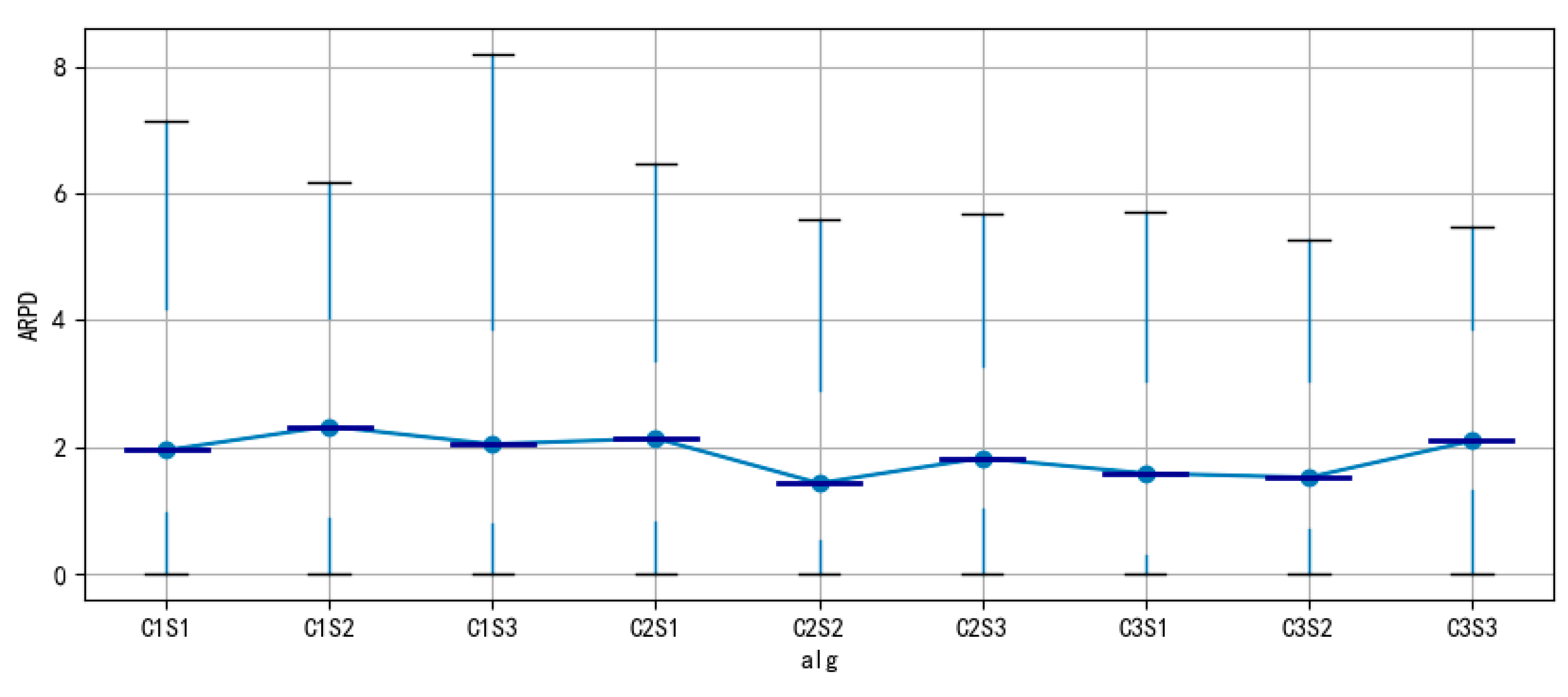
Evaluation of the performance of the nine heuristic algorithm strategies was conducted by comparing the relevant data for each strategy. Figure 3 presents the Average Percentage Relative Deviation (APRD) for all strategies. The results indicate that C1S3 exhibits the largest fluctuations, with a deviation span of approximately 8. In terms of numerical values, all strategies are closely clustered around 2, with C2S2 showing the smallest deviation and C1S2 showing the largest.

Table 1. The APRD value of each policy on the comparison instances.

Numerical Example		APRD									CT(s)
		C1S1	C1S2	C1S3	C2S1	C2S2	C2S3	C3S1	C3S2	C3S3
n	20	16.28	17.48	17.77	9.85	12.28	21.65	15.12	14.73	22.57	238.42
	30	32.41	21.09	28.42	28.03	7.11	20.69	21.17	23.95	27.08	357.78
	50	18.50	38.11	19.54	31.87	17.72	19.57	17.31	17.85	17.29	503.44
	100	23.08	20.09	29.91	24.18	28.64	19.46	13.54	17.94	24.86	1129.22
m	4	27.17	31.31	30.16	30.90	18.99	35.62	10.04	17.47	25.92	544.87
	6	35.18	38.35	36.34	36.75	21.22	30.80	25.92	26.91	36.17	631.96
	8	26.78	21.84	34.00	26.29	18.42	16.51	23.05	27.04	29.15	909.66
a	4	46.46	46.42	48.53	39.44	19.33	31.22	28.80	36.75	37.87	721.32
	6	27.65	32.14	25.11	35.29	30.23	29.70	25.00	22.13	31.39	725.63
	8	16.16	18.21	22.00	19.20	16.19	20.45	13.34	15.59	22.54	781.91

provides a more detailed description of the nine strategies, including both APRD and Computation Time (CT). The data presented were obtained from multiple experiments, comparing each strategy under different combinations of workpiece quantity (n), machine quantity (m), and AGV quantity (a). The table shows that CT increases as n, m, and a rise, particularly when n = 100, where CT reaches a maximum of 1129.22 s, significantly higher than the 238.42 s observed when n = 20. This indicates that an increase in the number of workpieces, machines, and AGVs directly affects the complexity of the scheduling problem, resulting in a substantial rise in computation time.

Overall, the data presented in the table highlight the strengths and weaknesses of the various heuristic strategies across different configurations. C2S2 consistently outperforms C1S1 in terms of APRD, especially when n = 3 and a = 6, where it approaches the optimal solution more closely. Within the same AGV selection strategy, changes in the AGV standby strategy led to an increase in APRD, suggesting that different standby strategies have a direct impact on the algorithm’s scheduling accuracy.

The average APRD values for the combinations of n, m, and a across the strategies C1S1, C1S2, C1S3, C2S1, C2S2, C2S3, C3S1, C3S2, and C3S3 are as follows: 22.57%, 24.20%, 23.91%, 23.48%, 16.44%, 20.34%, 16.78%, 18.62%, 22.95%, 29.71%, 30.50%, 33.50%, 31.31%, 19.54%, 27.64%, 19.67%, 23.81%, 30.41%, 30.09%, 32.26%, 31.88%, 31.31%, 21.92%, 27.12%, 22.38%, 24.82%, and 30.60%. Based on the average values across the strategies, C2S2 performs the best, followed by C3S1, while C1S2 and C1S3 perform comparatively poorly.

To further analyze the impact of different AGV selection strategies under varying operational constraints, we examined their performance across different job sizes, machine configurations, and AGV quantities. The results indicate that the choice of selection strategy significantly influences scheduling efficiency, particularly in scenarios with high job arrival rates or limited AGV availability. For instance, the Nearby Choice (NC) strategy exhibited superior performance in minimizing idle time when AGVs were scarce, whereas the Sequential Choice (SC) strategy provided more stable performance across different workload intensities. These findings highlight the importance of selecting an appropriate AGV scheduling strategy based on specific operational constraints. Future work could extend this analysis by incorporating additional real-time constraints such as AGV battery levels and dynamic traffic conditions.

To further evaluate the robustness of the proposed AGV scheduling strategies, we conducted a sensitivity analysis under varying operational conditions. Specifically, we analyzed the impact of different job sizes (n = {20, 30, 50, 100}), machine configurations (m = {4, 6, 8}), and AGV quantities (a = {4, 6, 8}) on scheduling performance. The results indicate that the Nearby Choice (NC) strategy performs best when AGVs are scarce, while the Sequential Choice (SC) strategy maintains stable performance across different machine and job configurations. Additionally, we observed that standby strategies significantly influence scheduling efficiency in high-load scenarios, whereby the Next Task Standby (NTS) strategy proved most effective in reducing idle time. This analysis highlights the importance of selecting AGV scheduling strategies based on specific production constraints, ensuring adaptability to different manufacturing environments. Future work could extend this study by incorporating real-time dynamic factors such as AGV battery life and unexpected job arrivals.

6.3. Comparison of Metaheuristics

The effectiveness of the proposed scheduling algorithms was assessed by comparing them with two well-established metaheuristic algorithms: Iterated Greedy (IG) and the Genetic Algorithm (GA). For the VND algorithm, no hyperparameters exist. For the IG algorithm and the GA, we used the best parameter settings suggested in the original paper for the parameters of the IG algorithm [30] and the GA [27].

Table 2. The average RPD and CPU time of the VND, IG, and GA algorithms on the comparison instances.

Numerical Example		VND		IG		GA
		ARPD (%)	CT (min)	ARPD (%)	CT (min)	ARPD (%)	CT (min)
n	20	0.07	3.02	3.41	18.78	2.97	18.00
	30	0.00	11.74	12.28	6.18	5.69	12.80
	50	0.00	11.64	74.01	17.50	65.55	21.83
m	4	0.03	7.21	17.74	13.35	13.65	16.32
	6	0.01	8.41	27.92	13.80	22.67	17.28
	8	0.00	10.59	37.42	13.49	31.06	18.12
a	4	0.03	7.84	26.52	14.06	21.67	17.03
	6	0.02	8.50	29.36	14.11	24.17	17.45
	8	0.02	9.31	32.11	14.18	26.62	17.90

shows that the ARPD of the VND algorithm is significantly lower than that of the IG algorithm and the GA across all test configurations. For instance, when the number of workpieces n = 20, the ARPD of the VND algorithm is 0.07%, while the ARPDs for IG and the GA are 3.41% and 2.97%, respectively. As n increases, for instance, when n = 50, the ARPD of the VND algorithm drops to 0%, while the ARPDs of IG and the GA sharply increase to 74.01% and 65.55%, respectively. Additionally, as the number of machines m and AGVs a increases, the ARPD of the VND algorithm remains consistently low. For instance, when m = 8 and a = 8, the ARPD of the VND algorithm is 0.00% and 0.02%, respectively, whereas the corresponding values for IG and the GA are 37.42%, 32.11% and 31.06%, 26.62%. These trends indicate that the VND algorithm demonstrates greater robustness and adaptability when handling more complex scheduling tasks.

In terms of CT, although the VND algorithm requires slightly more computation time in some configurations (for example, when n = 30, its CT is 11.74 min, higher than the 6.18 min for IG and 5.69 min for the GA), as the task size increases (for example, when n = 50), the CT of the VND algorithm is only 11.64 min, while the CT of IG and the GA rises to 17.50 min and 21.83 min, respectively. This performance shows that the VND algorithm outperforms the other two algorithms in terms of computational efficiency when handling larger problems.

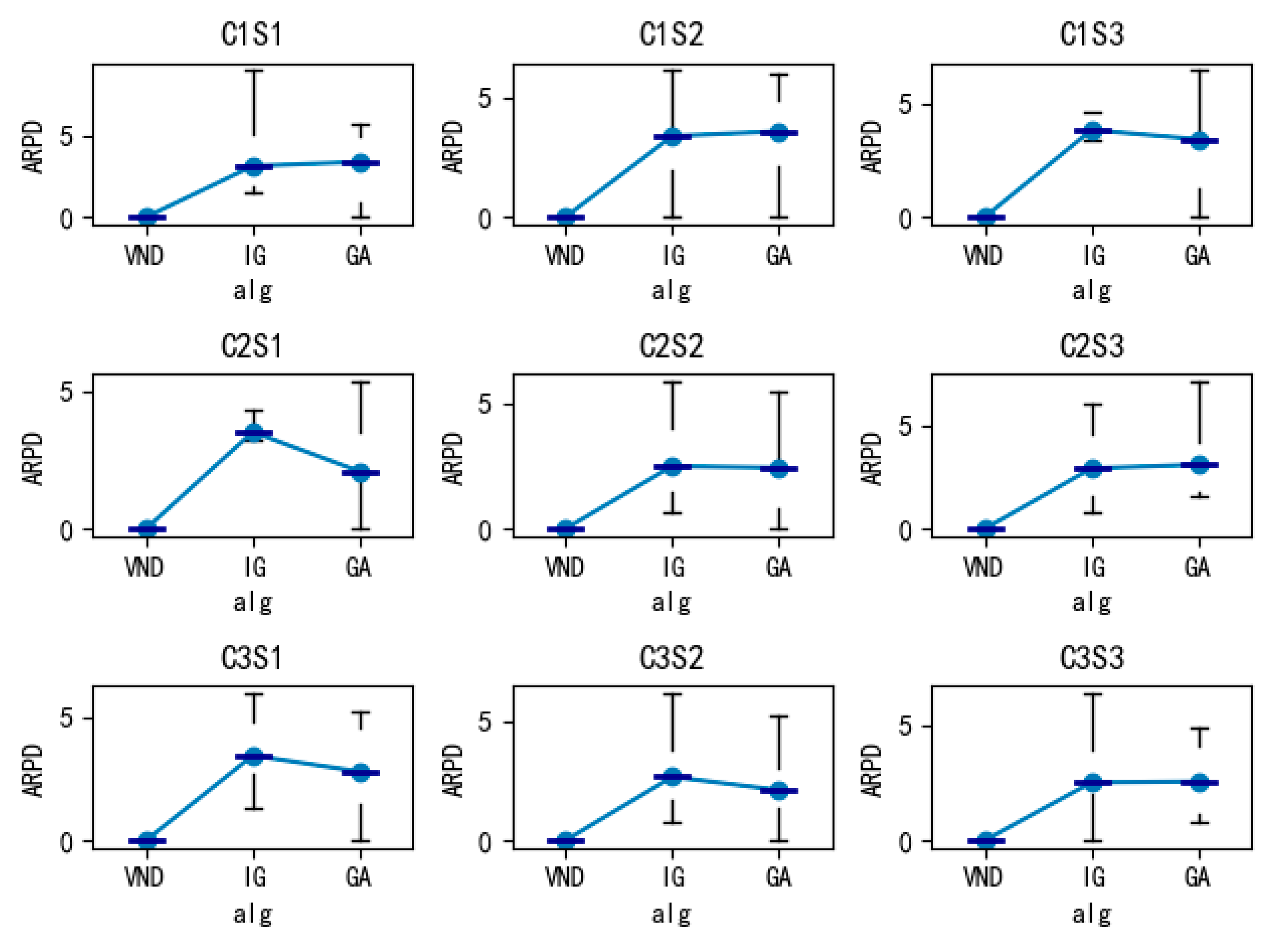
A comparison of the performance of the three algorithms under different strategies is shown in Figure 4. The ARPD values of the VND algorithm are consistently close to 0 across the nine strategies, indicating its significant superiority. In contrast, the ARPD values of IG and the GA fluctuate across strategies, with notably larger increases when strategy complexity is higher, suggesting that these algorithms have weaker adaptability to complex scheduling tasks.

The VND algorithm outperforms both the IG algorithm and the GA in scheduling accuracy and computational efficiency, highlighting its effectiveness in solving the pulsating assembly flow shop scheduling problem. While the proposed VND algorithm demonstrates strong performance in terms of scheduling accuracy and computational efficiency, certain limitations exist. The computational time increases with the problem size, particularly when the number of jobs and machines grows significantly. Although VND outperforms IG and the GA in large-scale instances, its efficiency could be further improved through parallel computing or hybrid optimization approaches. Additionally, the model assumes ideal conditions without considering unexpected disruptions such as machine breakdowns or AGV failures. Future research could explore robustness strategies, such as dynamic rescheduling and real-time decision-making, to enhance the model’s adaptability in real-world applications.

While this study focuses on optimizing AGV scheduling under predefined operational conditions, real-world uncertainties such as AGV speed variations, battery constraints, and machine breakdowns can significantly impact scheduling performance. Future research could extend the proposed model by incorporating adaptive scheduling mechanisms that dynamically adjust AGV assignments based on real-time battery levels and speed constraints. Additionally, integrating predictive maintenance strategies could enhance the model’s robustness against machine failure, further improving overall system reliability and efficiency.

7. Conclusions

This study addresses the pulsating assembly flow shop scheduling problem, with a particular focus on the integration of AGV scheduling. While existing research has primarily concentrated on solving the pulsating assembly flow shop scheduling problem, few studies have explored the specific role of AGV scheduling within this context. By filling this gap, our research not only enhances the efficiency of pulsating assembly line scheduling but also contributes to the broader trend of manufacturing toward “multiple varieties, small batches, and customization”.

In this study, we have established a comprehensive mathematical model to describe the scheduling problem, taking into account both product processing and AGV logistics. To optimize AGV scheduling, we designed three AGV selection strategies and three AGV standby strategies, each aimed at improving the overall production flow and reducing bottlenecks. Furthermore, we proposed metaheuristic algorithms to solve the problem efficiently under different production scenarios. The experimental results validate the effectiveness of the proposed AGV scheduling strategies and algorithms, demonstrating their ability to improve production efficiency, reduce AGV operational costs, and optimize the overall production rhythm. The outcomes of this research provide a valuable framework for enhancing the intelligence of pulsating assembly flow shops, offering practical solutions that align with modern manufacturing needs.

Future research could focus on enhancing the robustness and adaptability of the scheduling system by incorporating uncertainties in processing times, AGV performance, and other dynamic factors commonly encountered in real-world manufacturing environments. Additionally, integrating machine learning techniques or real-time data analytics for predictive scheduling could further optimize performance, enabling even greater efficiency and responsiveness in future pulsating assembly workshops. By addressing these uncertainties and leveraging advanced technologies, the system’s performance could be significantly improved to meet the demands of dynamic production environments.