Compact Multi-Channel Long-Wave Wideband Direction-Finding System and Direction-Finding Analysis for Different Modulation Signals

Abstract

This paper presents an optimized long-wave (10–300 kHz) wideband direction-finding system for scientific research. The antenna unit of the system comprises one vertical electric field sensor and two horizontal magnetic field sensors oriented in the north–south and east–west directions, respectively. The overall design prioritizes compactness, engineering feasibility, and ease of deployment, enabling the effective reception of long-wave radio signals within the 10–300 kHz range. The magnetic field sensitivity reaches $8fT/\sqrt{\mathrm{Hz}}@10\mathrm{kHz}$, while the electric field sensitivity achieves $3.2\mathsf{\mu }\mathrm{V}/\mathrm{m}/\sqrt{\mathrm{Hz}}@10\mathrm{kHz}$. The overall sensitivity of the receiver is $1\mathsf{\mu }\mathrm{V}$ (300 Hz bandwidth, 10 dB signal-to-noise ratio). The synchronization accuracy of the system is within 10 ns. Theoretically, with a baseline length of 5 km and a signal incidence angle ranging from 9.9° to 170.1°, the direction finding error is less than 2°. Additionally, direction-finding methods for MSK and ASK modulated signals are analyzed. To evaluate the system’s actual performance, initial measurements were conducted in Qingdao, Shandong.

1. Introduction

Research on long-wave radio science dates back to the late nineteenth century. Early telegraph operators occasionally heard sounds from telephone receivers, which they described as “clicks”, “grinders”, and “sizzles”. These sounds were generated by rapid changes or pulsations in currents caused by sunspots, geomagnetic currents, and auroras, which coupled with the telephone lines [1]. By the 1950s, research on long-wave radio had become a relatively mature field. The experiences gained during World War II subsequently highlighted the value of radio research in communication and navigation, sparking renewed interest in electromagnetic waves in the long-wave band. The demand for submarine navigation and communication, as well as reliable global military communication, has indirectly driven the development of VLF and ELF wave propagation theories and experiments over the past fifty years [2,3].

Before the advent of GPS, the United States established the first global navigation system, “Omega”, which consisted of eight VLF transmitter beacons [4]. However, with the emergence of GPS, long-wave navigation systems have gradually become supplementary in environments where GPS signals are limited or unavailable, due to GPS’s high precision and convenience.

Subsequent research has shown that VLF signals are highly suitable for remote sensing of the lower ionosphere (60–90 km) [5,6]. Measuring electron density in the lower ionosphere is difficult except through VLF techniques. High-frequency radio signals (e.g., those used in incoherent scatter radars) often suffer from insufficient reflection amplitudes, making them prone to being obscured by noise or interference. At these altitudes, the air density is too high for satellites, leading to excessive drag. Although rockets can provide satisfactory results, they are costly and can only offer instantaneous data, which are insufficient to address diurnal, seasonal, and latitudinal variations. In particular, the infrequent nighttime flights yield unreliable results [7].

Over the past thirty years, monitoring long-wave radio signals has primarily been used to study geophysical phenomena, such as lightning discharge signals [8,9,10,11,12,13,14], remote sensing and modeling of the ionospheric atmosphere [6,15,16,17,18], and observing relativistic runaway breakdown phenomena within thunderstorms [19]. As research into these phenomena progresses, the requirements for signal reception accuracy, sensitivity, signal-to-noise ratio, and bandwidth continue to rise. Increased sensitivity and bandwidth, along with more electromagnetic field components, enable the extraction of more information from long-wave signals, potentially revealing previously overlooked data. Furthermore, higher timing accuracy in multi-station cooperative direction finding and localization enhances both direction-finding and localization precision.

Previous studies have proposed and an deployed various long-wave receivers with different performance characteristics, tailored to specific scenarios. For example, the Los Alamos Sferic Array (LASA) has a bandwidth of 200 Hz to 500 kHz, a timing precision of $2\mathsf{\mu }\mathrm{s}$, and a sensitivity of $0.2\mathrm{V}/\left(\mathrm{m}\sqrt{\mathrm{Hz}}\right)$. It can record lightning discharges over thousands of kilometers, making it suitable for detecting lightning activity, localization, and conducting thunderstorm research [20]. Palmer Station in Antarctica provides a bandwidth of 100 Hz to 50 kHz, a timing precision of 100 ns, and records lightning discharges over thousands of kilometers for studies on the correlation between lightning discharges and terrestrial gamma-ray flashes (TGFs) [21,22]. A broadband digital low-frequency radio receiver with a bandwidth of 4 Hz to 400 kHz, a timing precision of 12 ns, and amplitude resolution of approximately $35\mathsf{\mu }\mathrm{V}/\left(\mathrm{m}\sqrt{\mathrm{Hz}}\right)$ was developed to observe radio signals from relativistic breakdown [19]. The Low Frequency Atmospheric Weather Electromagnetic System for Observation, Modeling, and Education (LF AWESOME) has a bandwidth of 0.5 kHz to 470 kHz, timing accuracy of 15–20 ns, magnetic field sensor sensitivity of $0.03fT/\sqrt{\mathrm{Hz}}$, and electric field sensor sensitivity of $0.677\mathrm{nV}/\left(\mathrm{m}\sqrt{\mathrm{Hz}}\right)$. It can be used for global detection of lightning discharges, monitoring transmission signals in the long- and medium-wave bands, undersea and subsurface sensing and communications, navigation and timing, and remote sensing of the ionosphere and magnetosphere [23,24].

Based on the previous literature, we summarize the overall performance of long-wave broadband receivers proposed in recent years, as shown in

Table 1. List of parameters for existing long-wave broadband receivers.

Reference	Year	Bandwidth	Electric/Magnetic Sensitivity	Antenna Size	Time Precision
Ref1 [19]	2009	4 Hz–400 kHz	N/A *	1.55 m	$\sim 12$ ns
Ref2 [25]	2010	300 Hz–30 kHz	$10fT/\sqrt{\mathrm{Hz}}$	2.6 m	$\sim 40$ ns
Ref3 [23]	2018	17–120 kHz	$1fT/\sqrt{\mathrm{Hz}}$	56 cm	15–20 ns
Ref4 [26]	2019	1–500 kHz	$7\mathrm{nV}/\mathrm{m}\sqrt{\mathrm{Hz}}$	1 m	15–20 ns
Ref5 [24]	2021	DC-470 kHz	$45\mathrm{nV}/\mathrm{m}\sqrt{\mathrm{Hz}}$	2 m	15–20 ns
This work	2025	10–300 kHz	$3.2\mathsf{\mu }\mathrm{V}/\mathrm{m}\sqrt{\mathrm{Hz}}$, $8fT/\sqrt{\mathrm{Hz}}$	20 cm(E-sensor), 35 cm (B-sensor)	<10 ns

* Not mentioned in the literature.

. This table briefly lists the parameters of sensors or receivers proposed in key studies over the past 20 years. Notably, some sensitivity parameters mentioned in the abstracts of these papers represent the theoretical limits achievable with large antenna configurations (25 m²) within the operating bandwidth, and sensitivity can fluctuate significantly across this bandwidth. This aligns with the focus of their research, which primarily examines the limits of such sensors, the effects of different design methods on sensor parameters, or requires a detailed study of specific physical phenomena. In contrast, our work primarily focuses on designing a more stable, compact long-wave receiver system with consistent sensitivity across the operating bandwidth. As a result, these parameters are not directly comparable to our work, and specific values should be carefully reviewed in the original papers for a more accurate comparison. The parameters provided in the table are those proposed in these studies and can be compared with our work, though they may differ from the general descriptions in prior works. However, both descriptions are correct in their respective contexts.

Based on the information from the table and the specific literature cited, in the work presented in this paper, we have designed a receiver with high synchronization accuracy and a minimal antenna size, while meeting the sensitivity requirements for the application. The high timing accuracy (10 ns) ensures higher direction-finding accuracy and resolution when constructing an interference network. The device’s ability to simultaneously collect horizontal magnetic field and vertical electric field signals, combined with its compact size, significantly enhances its versatility. Furthermore, our receiver exhibits an exceptionally flat sensitivity response across the operating bandwidth, a feature not present in most of the receivers discussed above. This ensures that wideband signals, such as lightning signals, remain undistorted across the entire bandwidth. The system can be effectively applied in direction finding, ionospheric remote sensing, lightning signal research, and other related fields.

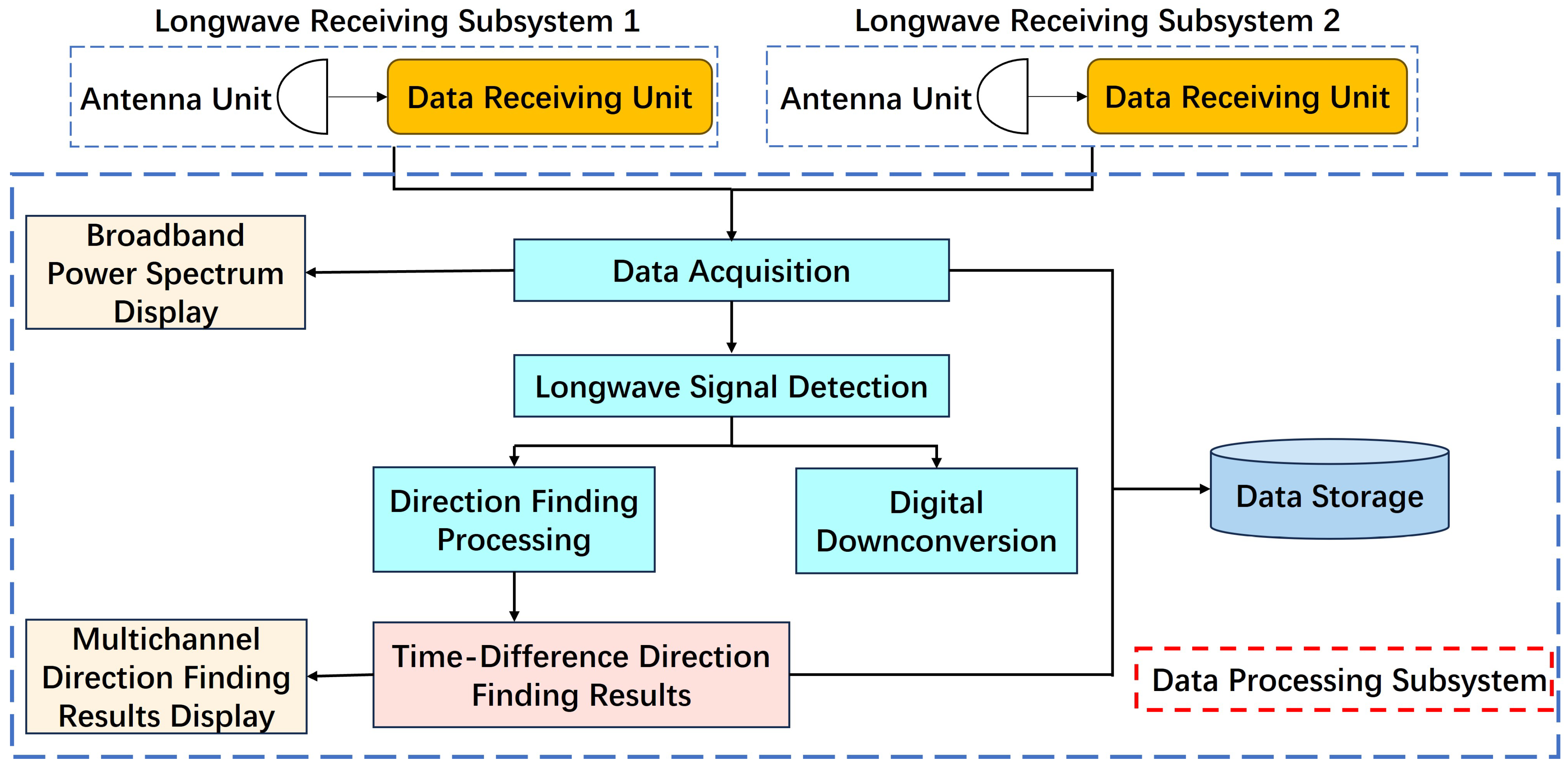
2. System Description

This paper first introduces the general design of the long-wave wideband direction-finding system, which primarily monitors long-wave communication signals globally. To achieve global coverage of submarine-to-submarine communication signals, it is necessary to leverage the transmission characteristics of electromagnetic waves in the Earth-ionosphere waveguide. Thus, the operating frequency must fall within the VLF/LF bands. Considering the operating frequencies of global long-wave radio stations, the system’s frequency coverage was selected to range from 10 kHz to 300 kHz. The LPF-B0R3+ low-pass filter was chosen to meet the bandwidth requirements and cover the primary target radios. To effectively sample long-wave signals within this frequency band, the sampling frequency, according to the sampling theorem, must be greater than twice the signal bandwidth. The system selects a 1 MHz sampling rate, providing slight redundancy without imposing excessive demands on subsequent processing and storage.

The long-wave wideband direction-finding system consists of two long-wave receiving subsystems and one data processing subsystem, as illustrated in the system block diagram in Figure 1.

The Longwave Receiving Subsystem is primarily used for long-wave broadband signal reception. Longwave Receiving Subsystem 1 and Subsystem 2 denote the main and ref receivers, respectively, with each subsystem comprising an antenna unit and a receiver unit. The antenna unit comprises one vertical electric field sensor and two horizontal magnetic field sensors. The electric field sensor is oriented vertically, while the magnetic field sensors are aligned in the north–south and east–west directions, respectively. For vertically polarized electromagnetic waves, the vertical electric field sensor exhibits high sensitivity and effectively captures weak signals. The horizontal magnetic field sensor measures the horizontal magnetic field, and the magnetic direction-finding method determines the orientation of long-wave signals, thereby providing more information [23,24]. The receiver unit collects the electromagnetic signals received by the antenna and transmits them to the data processing subsystem. The data processing subsystem comprises both hardware and software components. The hardware includes high-performance computers, storage devices, communication equipment, and display and control units. The software component is mainly utilized for wideband detection of long-wave signals, downconversion, outputting wideband power spectra, time-difference direction finding, display, storage, and transmission. As illustrated in Figure 2, which shows the schematic distribution of the long-wave receiving antennas, the vertical electric antenna uses parallel-plate capacitors and a low-noise amplifier to capture the vertical electric field component of long-wave signals. The horizontal magnetic antenna employs two orthogonal inductive magnetic antennas to separately receive the east–west and north–south components of the magnetic field. Each inductive magnetic antenna comprises multi-turn induction coils and low-noise circuitry.

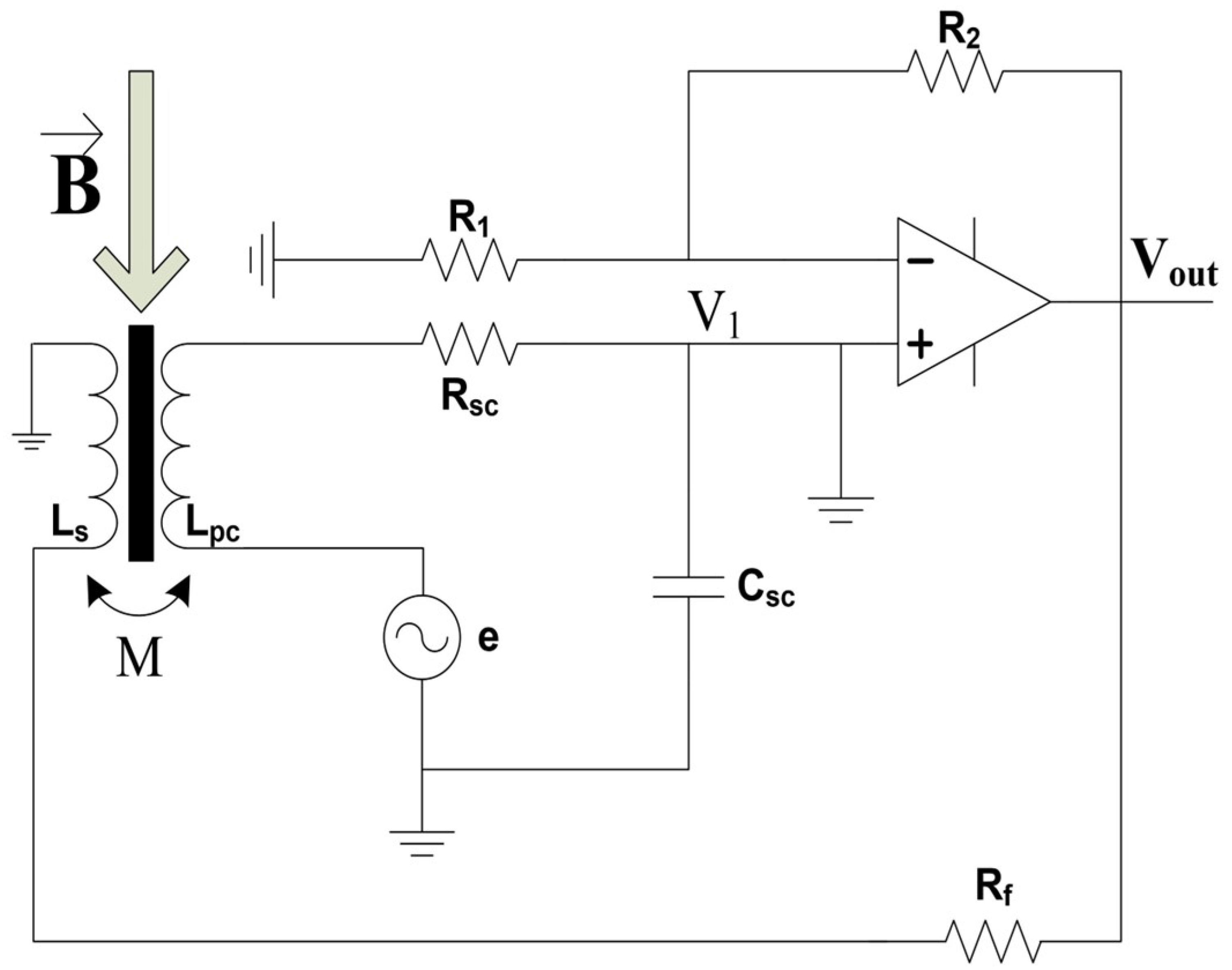
2.1. Horizontal Magnetic Field Sensor

Based on the system performance requirements outlined in the previous section and the design principles for magnetic field sensors, we have designed the system’s magnetic field sensor as follows. First, the equivalent circuit diagram of the flux negative feedback type broadband inductive magnetic field sensor, utilizing a feedback coil, is shown in Figure 3.

The primary coil is modeled as an inductor $L_{pc}$ in series with a resistor $R_{sc}$, which is then paralleled with a capacitor $C_{sc}$. The resistors $R_1$ and $R_2$ determine the amplification factor of the amplifier. The amplifier circuit primarily uses the instrumentation amplifier OPA128. The input voltage and current noise levels of the OPA128 are $8\mathrm{n}V/\sqrt{\mathrm{Hz}}$ and $300fA/\sqrt{\mathrm{Hz}}$, respectively, within a frequency range above 1 kHz. The output voltage $V_{out}$ is connected to the feedback coil through the feedback resistor $R_f$. The feedback coil has an inductance $L_s$ and its resistance is negligible. The feedback coil and the primary coil are mutually coupled with a mutual inductance M, where $L_{pc}=1.7H$, $C_{sc}=12pF$, and $R\_sc=51\Omega$.

Let the induced voltage in the coil be denoted as e:

$$e\left(\omega \right)=-j\omega {\mu }_{app}NSB,$$

(1)

where ${\mu }_{app}$ is the magnetic permeability, N is the number of turns of the coil, S is the effective cross-sectional area of the coil, and B is the magnetic field induction strength.

Therefore, when the gain applied to the induced voltage e is G, the output $V_{out}$ of this equivalent circuit in the frequency domain is expressed as follows:

$$V_{out}\left(\omega \right)={\displaystyle \frac{e\times G}{1+j\omega (C_{sc}{R}_{sc}+\frac{MG}{R_f+j\omega L_s})+{\left(j\omega \right)}^2{L}_{pc}{C}_{sc}}},$$

(2)

Analyzing the parameters in the denominator of equation, within the bandwidth range of 10 kHz to 300 kHz, the value of $R\_f$ is a few thousand ohms, and $L_s$ is on the order of tens of $\mu H$. In this range, $R_f$ is much larger than $j\omega L_s$, so $j\omega L_s$ can be neglected. Given that $C_{sc}=12pF$, $R\_sc=51\Omega$, M is a fraction of a few henries, and G is a large value in the thousands, the value of ${\displaystyle \frac{MG}{R_f}}$ is much larger than $C_{sc}{R}_{sc}$, so $C_{sc}{R}_{sc}$ can be ignored. After substituting these simplified results into Equation (2), the conversion factor $FS$ for the flux negative feedback-type broadband inductive magnetic field sensor in the low-frequency range up to 1000 kHz is

$$FS\left(\omega \right)={\displaystyle \frac{V_{out}}{B}}={\displaystyle \frac{-j\omega {\mu }_{app}NS\times G}{1+j\omega \frac{MG}{R_f}+{\left(j\omega \right)}^2{L}_{pc}{C}_{sc}}},$$

(3)

Analyzing the analytical expression of the conversion factor reveals that, in the low-frequency range, the amplitude of $FS$ increases linearly with frequency. As the frequency increases to a certain point, the amplitude of becomes frequency-independent and remains constant. When frequency increases further, the amplitude of decreases linearly with frequency. In summary, $FS$ forms a band-pass transfer function determined by two frequency inflection points.

Based on the aforementioned design principles, a wideband magnetic field sensor can be realized by adjusting the parameters of the feedback coil and circuit components. By optimizing the coil-circuit matching, the sensor’s operating frequency band is designed to be 10 kHz–300 kHz (within 3 dB attenuation), as shown in Figure 4.

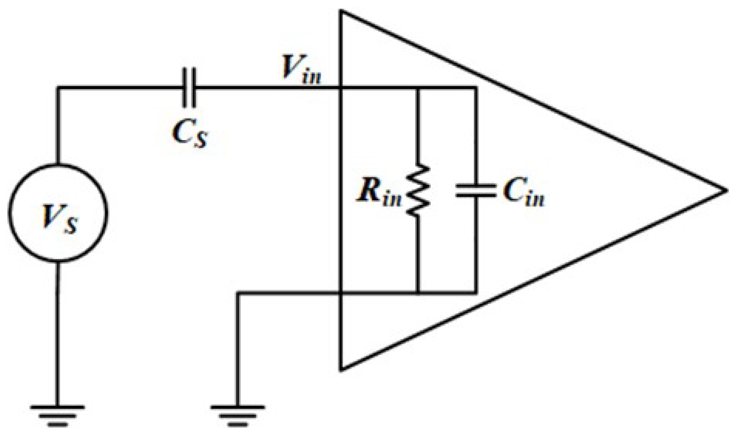
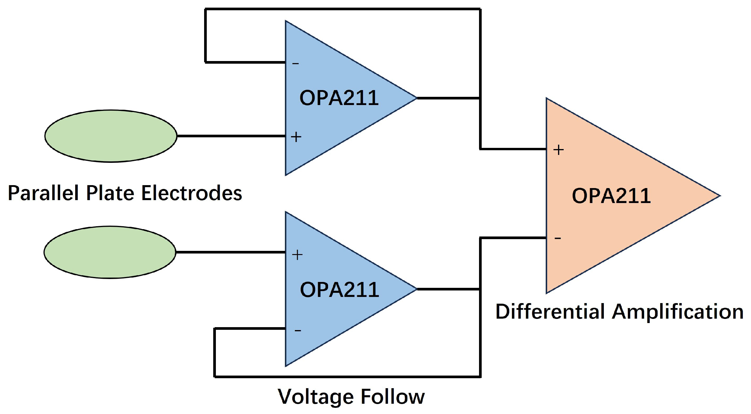
2.2. Vertical Electric Field Sensor

For electrodes placed in free space, the presence of an electric field causes a portion of charge to accumulate on the electrodes, thereby generating a certain potential. This can be equivalently modeled as a voltage source $V_s$. The electrodes themselves possess a certain capacitance $C_s$ relative to an infinite distance. The preamplifier can be equivalently represented as a parallel combination of input impedance $R_{in}$ and input capacitance $C_{in}$, as illustrated in Figure 5, which depicts the working principle of the electric field sensor.

According to the voltage division principle:

$${\displaystyle \frac{V_{in}}{V_s}}={\displaystyle \frac{Z_{in}}{Z_s+Z_{in}}}={\displaystyle \frac{\frac{l}{\frac{l}{R_{in}}+j\omega C_{in}}}{\frac{l}{j\omega C_s}+\frac{l}{\frac{l}{R_{in}}+j\omega C_{in}}}}={\displaystyle \frac{j\omega C_{\mathrm{s}}{R}_{in}}{l+j\omega C_{in}{R}_{in}+j\omega Cs{R}_{in}}},$$

(4)

If $\omega C_s{R}_{in}>>1$, then

$$\eta ={\displaystyle V_{in}{V}_s=\frac{C_s}{C_{in}+C_s}}$$

(5)

Since the sensor’s inherent capacitance is in the picofarad ($pF$) range, measuring low-frequency electric field signals (where $\omega$ is very small) requires $R_{in}$ to be extremely large (${10}^{10}\Omega$). Under these conditions, the reception efficiency is frequency-independent and primarily depends on the ratio of $C_s$ to $C_{in}$. It is evident from the above that a larger inherent capacitance of the electric field sensor leads to a higher input impedance of the preamplifier and a smaller input capacitance. This configuration facilitates the detection of low-frequency signals and improves coupling efficiency.

In this work, the schematic of the parallel-plate capacitors and low-noise amplification circuit is shown in Figure 6. The electric field sensor uses a bipolar plate made of FR4 copper-clad material with a diameter of 12 cm. The electric field antenna amplifier utilizes the OPA211, with a differential instrumentation amplification structure chosen to suppress common-mode noise.

Based on the design parameters, the inherent capacitance of the electrode plate, $C_s$, is approximately 10 pF (estimated based on the size of the electrode plates) [27], and the amplifier’s equivalent input impedance, $R_{in}$, is ${10}^{10}\Omega$. When $\omega C_s{R}_{in}=100$, the condition $\omega C_s{R}_{in}>>1$ is considered satisfied, resulting in a frequency $\omega$ of 1.6 kHz, which corresponds to the lower limit frequency. The upper limit frequency of the electric field sensor is determined by the cutoff frequency of the low-pass filter, which is set at 500 kHz in the design. The distance between the two pole plates is 20 cm, and the diameter of each pole plate is 15 cm (electrode plate and circuit boards combined), making the sensor compact. With the help of the front matching circuit, the antenna achieves an effective length of 1.5 m. Compared to a rod antenna, the capacitance between the two plates is larger, allowing the sensor to handle high-frequency measurements while maintaining better low-frequency performance. Overall, the electric field sensor operates within a frequency range of 1.6 kHz to 500 kHz, meeting the design requirements of 10 kHz to 300 kHz.

2.3. Sensitivity Analysis

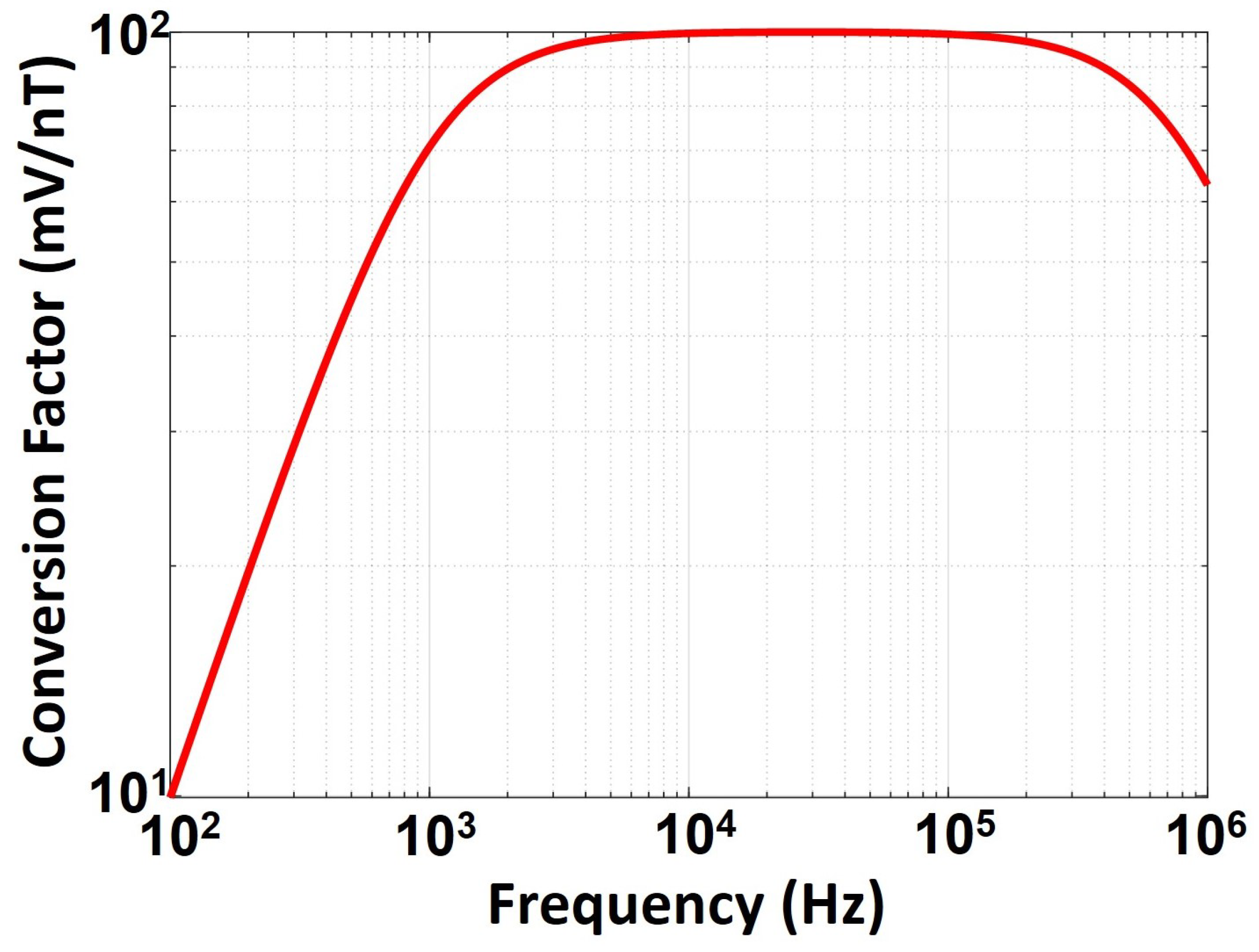
2.3.1. Magnetic Field Sensor Measurement Sensitivity Analysis

The sensitivity of a magnetic field sensor is defined as the power spectral density of its intrinsic noise in the frequency domain.

As a tool for measuring magnetic flux density, one of the most critical parameters of an inductive magnetic field sensor is its sensitivity, also referred to as equivalent input magnetic field noise. This type of noise originates internally within the sensor, including contributions from the coils and the amplification circuitry. Consequently, it cannot be mitigated through shielding layers and represents the inherent noise of the sensor, which can only be reduced but not entirely eliminated. Unfortunately, in practical applications, this noise often determines the minimum measurable magnetic flux density of the sensor, as well as the overall performance and suitability of the sensor for specific applications. Therefore, the equivalent input magnetic field noise is a critical consideration in both the analysis and design of the sensor.

Overall, inductive magnetic field sensors primarily comprise three major noise sources: coil resistor thermal noise (TR noise), circuit equivalent input voltage noise (CV noise), and circuit equivalent input current noise (CI noise).

In practice, noise sources are influenced by changes in sensor parameters, temperature variations, and frequency fluctuations. Therefore, the sensitivity of the sensor should be evaluated based on the actual design model and operating environment of the sensor, and ultimately verified through laboratory testing. The following sections analyze these three types of noise in detail.

• Coil Noise

For inductive magnetic field sensors, the coil comprises thousands of turns and can be modeled as a series combination of an ideal inductor ($L_{pc}$) and resistor ($R_{sc}$), which is then placed in parallel with an ideal capacitor ($C_{sc}$). Therefore, the noise introduced by the coil can be equivalently represented by the noise introduced by the resistor $R_{sc}$.

The thermal noise (TR noise) in the resistor arises from internal electronic motion. This type of noise was first experimentally verified by Johnson in 1928 and later theoretically derived by Nyquist. Therefore, the thermal noise in the resistor is also referred to as Nyquist noise. Let $k_B$ denote Boltzmann’s constant ($1.380649\times {10}^{-23}J/K$), and $T_c$ represent the absolute temperature. The equivalent input voltage noise ($e_{TR}$) at the sensor input due to TR noise is expressed as follows:

$$e_{TR}\left(f\right)=\sqrt{4k_B{T}_c{R}_{sc}}(V/\sqrt{\mathrm{Hz}}).$$

(6)

• Circuit-Induced Noise

Noise introduced by the amplification circuitry is one of the significant sources of noise in inductive magnetic field sensors and can generally be categorized into two types: equivalent input voltage noise and equivalent input current noise. In reality, all components on the circuit board, including both active and passive devices, contribute to the total noise, making it difficult to isolate and measure each component’s contribution individually. In this work, the overall noise from the circuit is equivalently modeled as a voltage source, namely CV noise ($e_{w1}$), and a current source, namely CI noise ($i_w$). These two noise sources are modeled and analyzed using direct measurement methods.

Similar to resistors, the noise introduced by the amplification circuit can also be decomposed into a white noise component and a $1/f$ noise component. The primary characteristic is that at high frequencies, white noise dominates, whereas at low frequencies, $1/f$ noise prevails. The frequency at which white noise equals $1/f$ noise is referred to as the noise corner frequency of the circuit’s equivalent input noise. For the sensors in this project, operating in the high-frequency range, the noise is predominantly dominated by the white noise from the first-order amplifier.

In summary, considering the operating environment of the sensors and omitting smaller noise terms, the equivalent input voltage noise ($e_{IM}$) of the inductive magnetic field sensor is given by

$$e_{IM}\left(f\right)=\sqrt{{e_{Rsc}}^2+{e_{w1}}^2+{\left[\right(i_w)\times |R_{sc}+j2\pi f{L}_{pc}\left|\right]}^2},$$

(7)

The equivalent input magnetic field noise ($b_{IM}$) is then

$$b_{IM}\left(f\right)={\displaystyle \frac{e_{IM}}{|2\pi f{\mu }_{app}NS|}}$$

(8)

Based on the above analysis and the parameters provided in Section 2.1, an inductive magnetic field sensor is designed in this project to serve as the magnetic field antenna for a long-wave broadband receiver, with its noise level shown in Figure 7.

Magnetic field sensors must be tested in an environment free from magnetic noise. In this study, a magnetically shielded room, isolated from urban electromagnetic interference, with a grounded enclosure was used. The chamber is made of high-permeability and high-inductance materials, providing a shielding factor greater than 90 dB at frequencies above 10 Hz, which effectively shields against low-frequency electric and magnetic field noise. The sensor under test was placed at the center of the shielded room, and measurements were taken using a digital signal analyzer (Agilent, Santa Clara, CA, USA, 35,670 A) outside the room. The results are shown in Figure 8.

As shown, the sensor’s noise power spectral density is less than $8fT/\sqrt{\mathrm{Hz}}@10kHz$, meeting the design requirements.

2.3.2. Electric Field Sensor Measurement Sensitivity Analysis

The electric field sensor in this design uses the parallel-plate capacitor principle to measure electric fields, consisting of a pair of parallel plate electrodes and the associated amplification circuitry. The amplification circuit is implemented using a two-stage amplification method, where the first stage is a voltage follower and the second stage is a differential amplifier with a gain of 37.5 times. While the amplification circuit enhances the electric field signal and improves the sensor’s frequency characteristics, it also introduces noise, thereby limiting the sensor’s electric field detection sensitivity.

The primary source of antenna noise is thermal noise, defined by $e_d=\sqrt{4kT{R}_a}$, where k is Boltzmann’s constant, T is the ambient temperature in Kelvin, and $R_a$ is the antenna’s ohmic resistance. However, in this frequency band, noise from voltage-following and back-amplification circuits dominates the antenna noise [24,26].

The test results from the shielded room are shown in Figure 9, with the test method being similar to that used for magnetic sensors.

It can be seen that the output voltage noise of the electric field sensor (including the amplifier circuit) reaches $3.2\mathsf{\mu }\mathrm{V}/\mathrm{m}\sqrt{\mathrm{Hz}}@10kHz$.

2.3.3. Receiver Sensitivity Analysis

Sensitivity represents a receiver’s ability to detect weak signals. The weaker the signal a receiver can detect, the higher its sensitivity. The sensitivity of a digital receiver is typically expressed as the minimum detectable signal power ($S_{min}$). When the input signal power to the receiver reaches $S_{min}$, the receiver can successfully detect and output the signal. If the signal power falls below this threshold, the signal becomes submerged in noise.

The sensitivity of a receiver is not only related to the signal bandwidth but also depends on factors such as the sampling frequency and the noise figure of the analog front-end. In this analysis, we primarily examine the relationship between receiver sensitivity and reception bandwidth. According to the actual application and design experience requirements, under the conditions of a 300 Hz bandwidth and a 10 dB signal-to-noise ratio, the receiver detection sensitivity is required to be $1\mathsf{\mu }\mathrm{V}$ to meet the equipment specifications.

If the detection sensitivity index is based on a peak value of $1\mathsf{\mu }\mathrm{V}$ and the matching resistance is $50\Omega$, the corresponding signal power is

$$P_{signal}={\displaystyle \frac{V_{\mathrm{rms}}^2}{R}}={\displaystyle \frac{{(0.707\times {10}^{-6}\mathrm{V})}^2}{50\Omega }}=-110\mathrm{dBm},$$

(9)

where $V_{rms}$ is the effective voltage and R is the matching resistance.

When the receiving bandwidth is 300 Hz, the receiver thermal noise can be theoretically calculated as

$$\begin{array}{cc}\hfill P_n\left(\mathrm{dBm}\right)& =P_{n0}(\mathrm{dBm}/\mathrm{Hz})+10{log}_{10}\left(B\right)\hfill \\ & =-174dBm/Hz+10{log}_{10}(300Hz)\hfill \\ & \approx -149\mathrm{dBm},\hfill \end{array}$$

(10)

where −174 dBm/Hz is the thermal noise power density per Hz bandwidth at room temperature (∼290 K), derived from basic theoretical thermal noise calculations, and B is the signal bandwidth.

Additionally, the noise figure (NF) of the analog front-end is relatively high due to the variable gain characteristic of the receiver. The noise figure is defined as the ratio of the additional noise introduced by the receiver front-end to the thermal noise, typically expressed in dB. In this paper, based on the system design and the specifications of the analog front-end components, a noise figure of 12 dB is assumed. Additionally, a minimum signal-to-noise ratio (SNR) threshold is required to ensure reliable signal detection. A signal-to-noise ratio (SNR) criterion of 10 dB is chosen in this paper, a common design parameter used to ensure the signal is significantly above the noise level for accurate detection by the receiver. Combining these factors, the overall thermal noise power $P_{total}$ of the circuit is calculated as follows:

$$\begin{array}{cc}\hfill P_{\mathrm{total}}\left(\mathrm{dBm}\right)& =P_n\left(\mathrm{dBm}\right)+NF\left(\mathrm{dB}\right)+SNR\left(\mathrm{dB}\right)\hfill \\ & =-149\mathrm{dBm}+12\mathrm{dB}+10\mathrm{dB}=-127\mathrm{dBm},\hfill \end{array}$$

(11)

In this design, the ADC is a 24-bit converter with a maximum effective dynamic range of 103 dB and an input range of ±2.5 V. Consequently, the corresponding quantization noise power is −98 dBm, which is significantly higher than the overall circuit thermal noise. To ensure accurate signal detection, the signal power should exceed the maximum noise power by 10 dB. When the gain of the pre-amplification analog circuit exceeds 22 dB, a $1\mathsf{\mu }\mathrm{V}$ signal is amplified to above −88 dBm, thereby satisfying the sensitivity detection requirements.

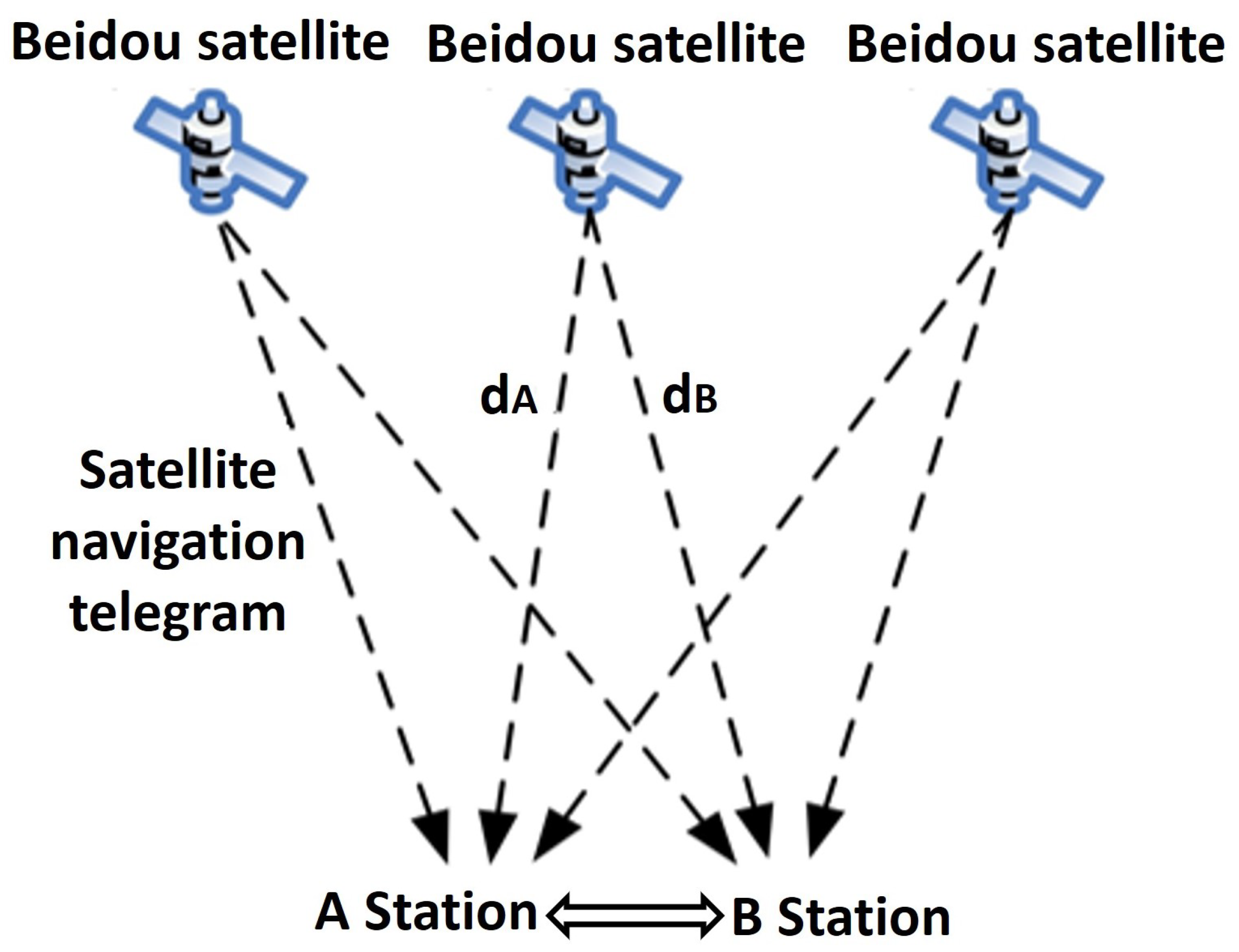
2.4. Time Synchronization Precision

Time synchronization precision refers to the accuracy of synchronization between multiple receivers. This metric depends on the synchronization precision of the timing modules. In this design, the synchronization precision requirement between the two re-ceivers is within 10 ns. Therefore, the BeiDou co-view time-frequency transfer technology is proposed to synchronize the two long-wave receiving subsystems [28,29,30].

The principle of BeiDou co-view time-frequency transfer is shown in Figure 10:

The BeiDou receivers are positioned at two known locations, A and B. Let the clock time at location A be $t_A$, the clock time at location B be $t_B$, and the BeiDou satellite time be $t_{BD}$. Let $d_A$ and $d_B$ denote the path delays from the satellite to locations A and B, respectively. The co-view receivers at locations A and B simultaneously receive signals from the same satellite. The second pulses output by the receivers, representing BeiDou time, are sent to a high-precision time interval measurement module and compared with the local clock pulses. This process produces the time difference count values $\Delta t_{ABD}$ and $\Delta t_{BBD}$ for the receivers at locations A and B relative to the satellite, as expressed in the following equations:

$$\begin{array}{c}\hfill \Delta t_{ABD}=t_A-(t_{BD}+d_A),\\ \hfill \Delta t_{BBD}=t_B-(t_{BD}+d_B),\end{array}$$

(12)

The data from locations A and B are transmitted to each other’s computers through a communication link. The path delays $d_A$ and $d_B$ can be calculated using ephemeris data. By subtracting the two equations above, the time difference between the two locations can be calculated, as shown below:

$$\Delta t_{ABD}-\Delta t_{BBD}=(t_A-t_{BD}-d_A)-(t_B-t_{BD}-d_B)=(t_A-t_B)-(d_A-d_B),$$

(13)

BeiDou co-view time-frequency transfer eliminates clock discrepancies by establishing co-view data communication and employing a weighted mutual difference algorithm for co-view fitting values. This reduces path delay errors effectively.

In this design, BeiDou co-view technology is applied using an optimized high-precision clock disciplining algorithm to tame the built-in high-stability crystal oscillator, thereby achieving high-precision BeiDou timing services. The absolute timing precision is better than 10 ns, and the system has strong independent time-keeping capabilities. Additionally, it outputs timing signals, including 10 MHz and 1 PPS, meeting the precise timing and synchronization requirements of the long-wave receivers.

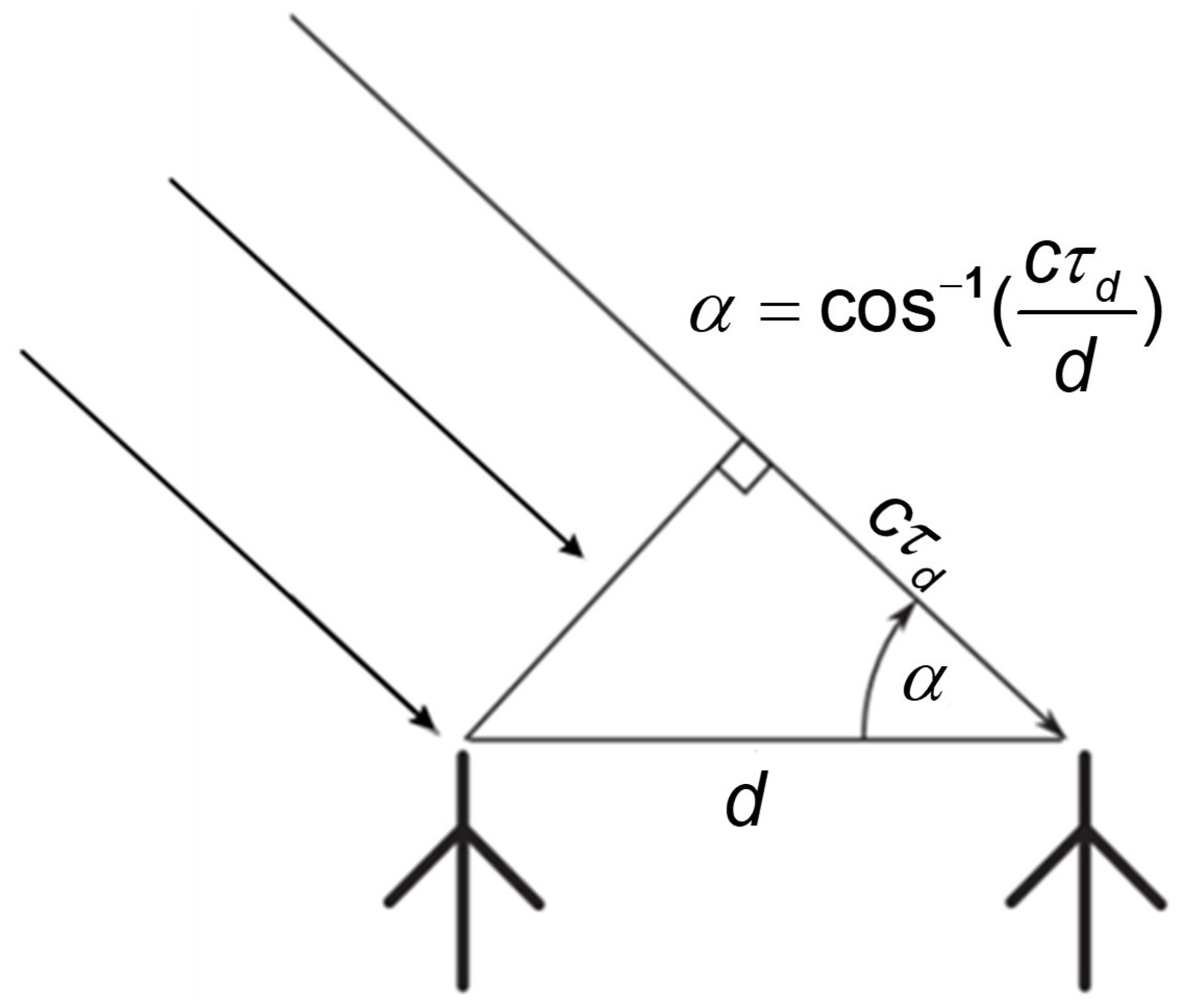
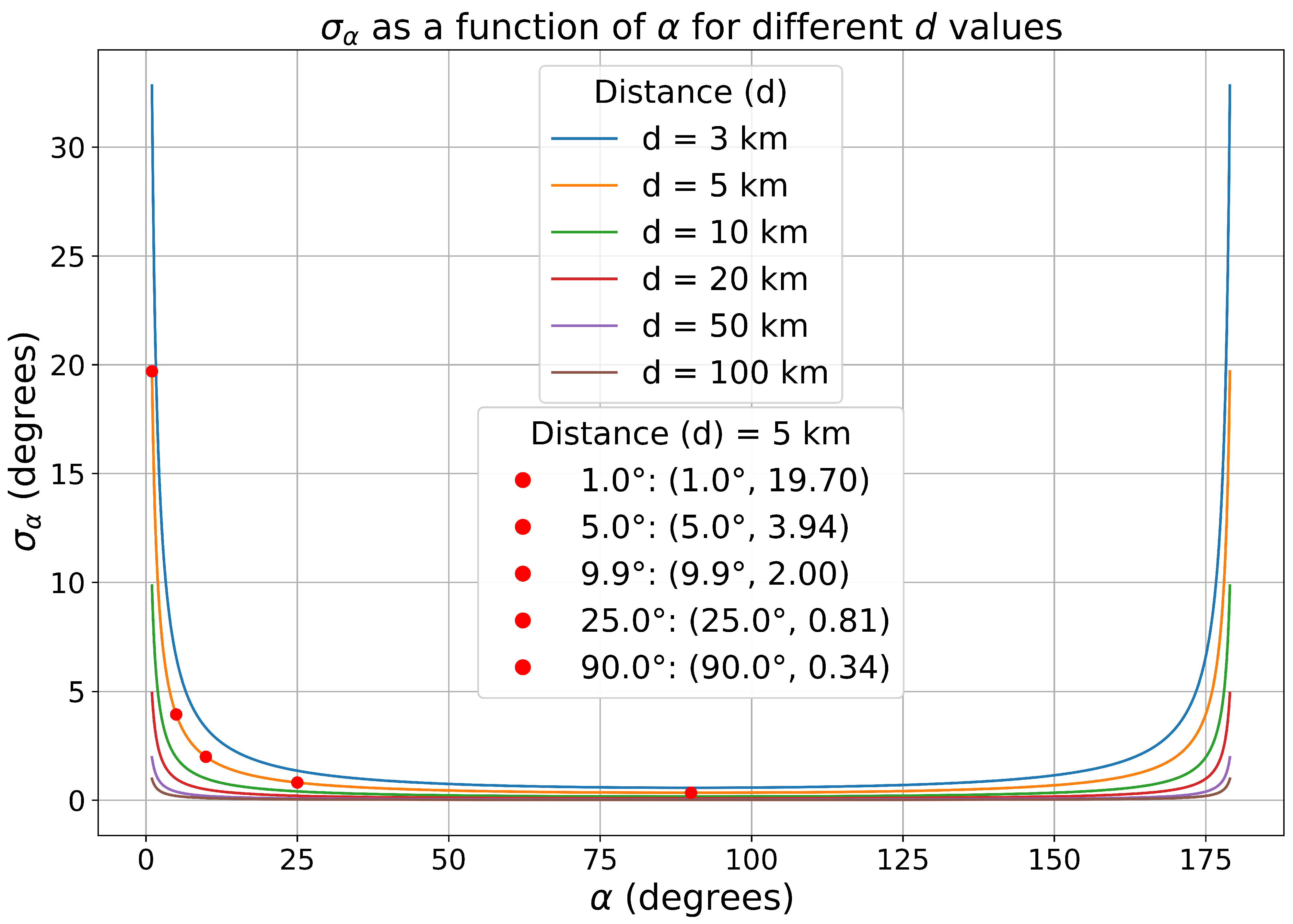
2.5. Direction-Finding Accuracy

For two array elements spaced by a distance d, as shown in Figure 11, the time difference $\tau$ of long-wave signals arriving at the elements is related to the angle of arrival $\alpha$ as follows:

$$\alpha ={cos}^{-1}\left({\displaystyle \frac{c{\tau }_d}{d}}\right),$$

(14)

where c is the speed of light. By calculating the time difference ${\tau }_d$, the direction cosine $cos\alpha$ of the arriving long-wave signal can be determined.

By taking the partial derivatives of the parameters with respect to the errors, the error propagation function is derived as follows:

$${\sigma }_{\alpha }={\displaystyle \frac{\tau {\sigma }_c+c{\sigma }_{\tau }+\frac{c\tau }{d}{\sigma }_d}{\sqrt{d^2-{\left(c{\tau }_d\right)}^2}}},$$

(15)

where ${\sigma }_{\alpha }$ represents the direction finding error, and ${\sigma }_{\tau }$ denotes the time difference error, which contributes the system’s inherent error. The baseline length error ${\sigma }_d$ can be neglected under precise measurement conditions, and ${\sigma }_c$ represents the velocity error caused by the propagation of electromagnetic waves in the ionosphere-ground waveguide model. In traditional systems, ${\sigma }_c$ is often neglected or set to a specific value of the speed of light (e.g., $0.9922c$), and we have

$$\tau ={\displaystyle \frac{d·cos\alpha }{c}},$$

(16)

By substituting Equation (16) into Equation (15), neglecting ${\sigma }_c$ and ${\sigma }_d$, and treating ${\sigma }_{\tau }$ as a fixed value, ${\sigma }_{\alpha }$ becomes a function of

$${\sigma }_{\alpha }={\displaystyle \frac{c·{\sigma }_{\tau }}{d·sin\alpha }}(0<\alpha <{180}^{\circ }),$$

(17)

From the above equation, it is evident that for a fixed system, without considering errors in the speed of light, both the speed of light c and the baseline length d are fixed values. The direction finding error ${\sigma }_{\alpha }$ is determined by the incident angle $\alpha$ at which the signal arrives at the array elements and the time difference error ${\sigma }_{\tau }$. The time difference error includes both the receiver synchronization error and the propagation error: the receiver synchronization error is 10 ns, and the propagation error is typically assumed to be $1\mathsf{\mu }\mathrm{s}$ per 100 km. Therefore, for a site spacing of 5 km, the propagation error is approximately 50 ns. Considering other uncontrollable factors, with a total time difference error of 100 ns, the distribution of ${\sigma }_{\alpha }$ with $\alpha$ is shown in Figure 12. The longer the baseline length, the better the direction finding error ${\sigma }_{\alpha }$. Considering site and terrain constraints, the baseline length is set to approximately 5.18 km. At this baseline length, when the signal incident angle is between 9.9° and 170.1°, the direction finding error is less than 2°, which is within the acceptable range.

2.6. Direction Finding of ASK and MSK Modulated Signals

In long-wave radio direction finding, different modulation methods may require distinct techniques. In the ASK modulation mode, which primarily modulates the signal amplitude without affecting the carrier phase, the arrival time difference can be directly calculated from the phase difference of the narrowband data measured by the two receivers:

$${\tau }_d\left(t\right)={\displaystyle \frac{\Delta {\varphi }_0\left(t\right)}{2\pi f_c}},$$

(18)

where $\Delta {\varphi }_0\left(t\right)$ represents the phase difference between the two receivers at time t, and $f_c$ is the carrier frequency of the wave source. By combining Equations (14) and (18), the angle of the wave source can be determined. However, it is important to note that during low-power periods of ASK modulation, noise can significantly affect the signal phase. Therefore, stable phase differences must be extracted during high-power periods for accurate direction finding.

However, the MSK modulation method can affect the signal phase due to its frequency modulation and the path delay in receiving the two MSK signals. When calculating the phase difference between the two receivers, this difference includes not only the carrier phase shift but also the phase shift introduced by the MSK baseband signal [16]. If the phase of the narrowband signal is directly used for time difference estimation, errors will occur. The ideal MSK modulated signal is shown below:

$$s\left(t\right)=cos\left[2\pi f_{c}t+b\left(t\right){\displaystyle \frac{\pi t}{2T}}+\theta \left(t\right)\right],$$

(19)

where T is the symbol period, and $b\left(t\right)$ represents the bit stream,

$$\begin{array}{cc}\hfill & b\left(t\right)=\left\{\begin{array}{cc}+1,\hfill & a_I\left(t\right)\ne a_Q\left(t\right),\hfill \\ \\ -1,\hfill & a_I\left(t\right)=a_Q\left(t\right),\hfill \end{array}\right.\hfill \\ \hfill & \theta \left(t\right)=\left\{\begin{array}{cc}0,\hfill & a_I\left(t\right)=1,\hfill \\ \\ \pi ,\hfill & a_I\left(t\right)=-1.\hfill \end{array}\right.\hfill \end{array}$$

(20)

with ${\alpha }_I$ and ${\alpha }_Q$ representing in-phase and quadrature coding, respectively. The phase of the baseband signal is then

$${\varphi }_{\mathrm{MSK}}\left(t\right)={\displaystyle \frac{\pi }{2T}}{\int }_{-\infty }^{t}b\left(t\right)dt=b\left(t\right){\displaystyle \frac{\pi t}{2T}}+\theta \left(t\right),$$

(21)

Since the signal sources and device parameters of the two receivers are identical, and the propagation path of one receiver is an extension of the other, the signals received by the two receivers can be expressed as follows:

$$\begin{array}{cc}& s_1\left(t\right)=cos\left[2\pi f_c(t-{\tau }_0\left(t\right))+{\varphi }_{\mathrm{MSK}}(t-{\tau }_1\left(t\right))\right],\hfill \\ & s_2\left(t\right)=cos\left[2\pi f_c(t-{\tau }_0\left(t\right)-{\tau }_d\left(t\right))+{\varphi }_{\mathrm{MSK}}(t-{\tau }_1\left(t\right)-{\tau }_d\left(t\right))\right],\hfill \end{array}$$

(22)

where ${\tau }_0$ and ${\tau }_1$ represent the propagation delays caused by the common path and device effects, respectively, at that moment, and ${\tau }_d$ is the time difference when the signal reaches the two receivers. The instantaneous phase difference between the two signals at this moment can be expressed as follows:

$$\begin{array}{cc}\hfill \Delta \varphi \left(t\right)& =\left\{2\pi f_c\left(t-{\tau }_0\left(t\right)\right)+{\varphi }_{\mathrm{MSK}}\left(t-{\tau }_1\left(t\right)\right)\right\}\hfill \\ & -\left\{2\pi f_c\left[\left(t-{\tau }_0\left(t\right)\right)-{\tau }_d\left(t\right)\right]+{\varphi }_{\mathbf{MSK}}\left[\left(t-{\tau }_1\left(t\right)\right)-{\tau }_d\left(t\right)\right]\right\}\hfill \\ & =\underset{\mathit{carrier}\mathit{phase}\mathit{difference}}{\underbrace{2\pi f_c{\tau }_d\left(t\right)}}+\underset{\mathrm{MSK}\mathrm{baseband}\mathrm{phase}\mathrm{difference}}{\underbrace{\left[{\varphi }_{\mathrm{MSK}}\left(t-{\tau }_1\left(t\right)\right)-{\varphi }_{\mathrm{MSK}}\left(\left(t-{\tau }_1\left(t\right)\right)-{\tau }_d\left(t\right)\right)\right]}}\hfill \\ & =2\pi f_c{\tau }_d\left(t\right)+\Delta {\varphi }_{\mathrm{MSK}}\left(t\right),\hfill \end{array}$$

(23)

hence,

$${\tau }_d\left(t\right)={\displaystyle \frac{\Delta \varphi \left(t\right)-\Delta {\varphi }_{\mathrm{MSK}}\left(t\right)}{2\pi f_c}},$$

(24)

where,

$$\begin{array}{cc}\hfill \Delta {\varphi }_{\mathrm{MSK}}\left(t\right)& ={\displaystyle \frac{\pi }{2T}}{\int }_{-\infty }^{t-{\tau }_1\left(t\right)}b\left(t\right)dt-{\displaystyle \frac{\pi }{2T}}{\int }_{-\infty }^{t-{\tau }_1\left(t\right)-{\tau }_d\left(t\right)}b\left(t\right)dt\hfill \\ & ={\displaystyle \frac{\pi }{2T}}\left[{\int }_{t-{\tau }_1\left(t\right)-{\tau }_d\left(t\right)}^{t-{\tau }_1\left(t\right)}b\left(t\right)dt\right].\hfill \end{array}$$

(25)

To simplify the expression, assuming ${\tau }_d$ is a small quantity (i.e.,${\tau }_d\ll T$) and that ${\tau }_1$ changes slowly, it can be approximated that $b\left(t\right)$ remains constant within the interval $[t-{\tau }_1\left(t\right)-{\tau }_d\left(t\right),t-{\tau }_1\left(t\right)]$.

Let $b(t-{\tau }_1\left(t\right))=b_k$; that is, the current symbol is $b_k$, then

$$\Delta {\varphi }_{\mathrm{MSK}}\left(t\right)\approx {\displaystyle \frac{\pi }{2T}}·b_k·{\tau }_d\left(t\right).$$

(26)

This approximation holds when the path delay ${\tau }_d$ is much smaller than the symbol period T. For common MSK signals, T typically ranges between 4–10 ms. In this system, the maximum path delay ${\tau }_d$ is approximately $17.3\mathsf{\mu }\mathrm{s}$, which satisfies the approximation condition. At this time,

$${\tau }_d\left(t\right)\approx {\displaystyle \frac{\Delta \varphi \left(t\right)}{2\pi f_c+\frac{\pi }{2T}·b_k}}.$$

(27)

Since ${\displaystyle \frac{\pi }{2T}}·b_k$ is much smaller than $2\pi f_c$, and $b(t-{\tau }_d)=\pm 1$, over a certain period of integration, if the number of positive and negative terms of $b_k$ is roughly equal and $\Delta \varphi$ is not extremely small, this term can be neglected. Therefore,

$${\tau }_d\left(t\right)\approx {\displaystyle \frac{\Delta \varphi \left(t\right)}{2\pi f_c}}.$$

(28)

To more effectively eliminate the influence of term ${\displaystyle \frac{\pi }{2T}}·b_k$, i.e., to remove the MSK phase modulation and better track the phase variation of the carrier frequency, we set

$$\begin{array}{cc}\hfill {\varphi }_0\left(t\right)& \equiv -2\pi f_c{\tau }_0\left(t\right),\hfill \\ \hfill {\varphi }_1\left(t\right)& \equiv -{\displaystyle \frac{\pi {\tau }_1\left(t\right)}{2T}}.\hfill \end{array}$$

(29)

The MSK signal with delay received by the receiver can be expressed as follows:

$$\begin{array}{cc}\hfill x\left(t\right)& =cos\left[2\pi f_{c}t+{\varphi }_0\left(t\right)+{\varphi }_{\mathrm{MSK}}(t-{\tau }_1\left(t\right))\right]\hfill \\ & =cos\left[2\pi f_{c}t+{\varphi }_0\left(t\right)+b(t-{\tau }_1\left(t\right))\left({\displaystyle \frac{\pi t}{2T}}+{\varphi }_1\left(t\right)\right)+\theta (t-{\tau }_1\left(t\right))\right].\hfill \end{array}$$

(30)

After performing a series of operations such as downconversion and filtering on the wideband signal, we obtain

$$z\left(t\right)=A\left(t\right)e^{j\varphi \left(t\right)}=A\left(t\right)exp\left[j{\varphi }_0+j{\varphi }_{\mathrm{MSK}}(t-\tau )\right].$$

(31)

By squaring the signal $z\left(t\right)$, since $2\theta (t-{\tau }_1\left(t\right))=0\mathrm{or}2\pi$, the $\theta (t-{\tau }_1\left(t\right))$ term can be eliminated, resulting in

$$\angle {\left[z\left(t\right)\right]}^2=2{\varphi }_0\left(t\right)\pm {\displaystyle \frac{\pi t}{T}}\pm 2{\varphi }_1.$$

(32)

In this equation, the signs of the latter two terms are determined by the instantaneous symbol of $b(t-{\tau }_1\left(t\right))$. Let

$${\varphi }_{\pm }=2{\varphi }_0\pm 2{\varphi }_1,$$

(33)

Assuming that ${\varphi }_0$ and ${\varphi }_1$ remain stable during the integration period, we have

$${\varphi }_{\pm }=\angle \left\{{\displaystyle \frac{1}{t_1-t_0}}{\int }_{t_0}^{t_1}{\displaystyle \frac{{\left[z\left(t\right)\right]}^2}{{\left[A\left(t\right)\right]}^2}}{e}^{\mp j\pi t/T}\mathrm{d}t\right\}.$$

(34)

By estimating ${\varphi }_{\pm }$ within a given time range, the carrier phase ${\varphi }_0$ can be estimated as follows:

$$\widehat{{\varphi }_0}={\displaystyle \frac{{\varphi }_{+}+{\varphi }_{-}}{4}}.$$

(35)

Thus, by isolating and differencing the MSK carrier phases of the signals received by the two receivers, the time difference can be more accurately estimated:

$${\tau }_d\left(t\right)=-{\displaystyle \frac{\Delta {\widehat{\varphi }}_0\left(t\right)}{2\pi f_c}}.$$

(36)

3. Results and Discussion

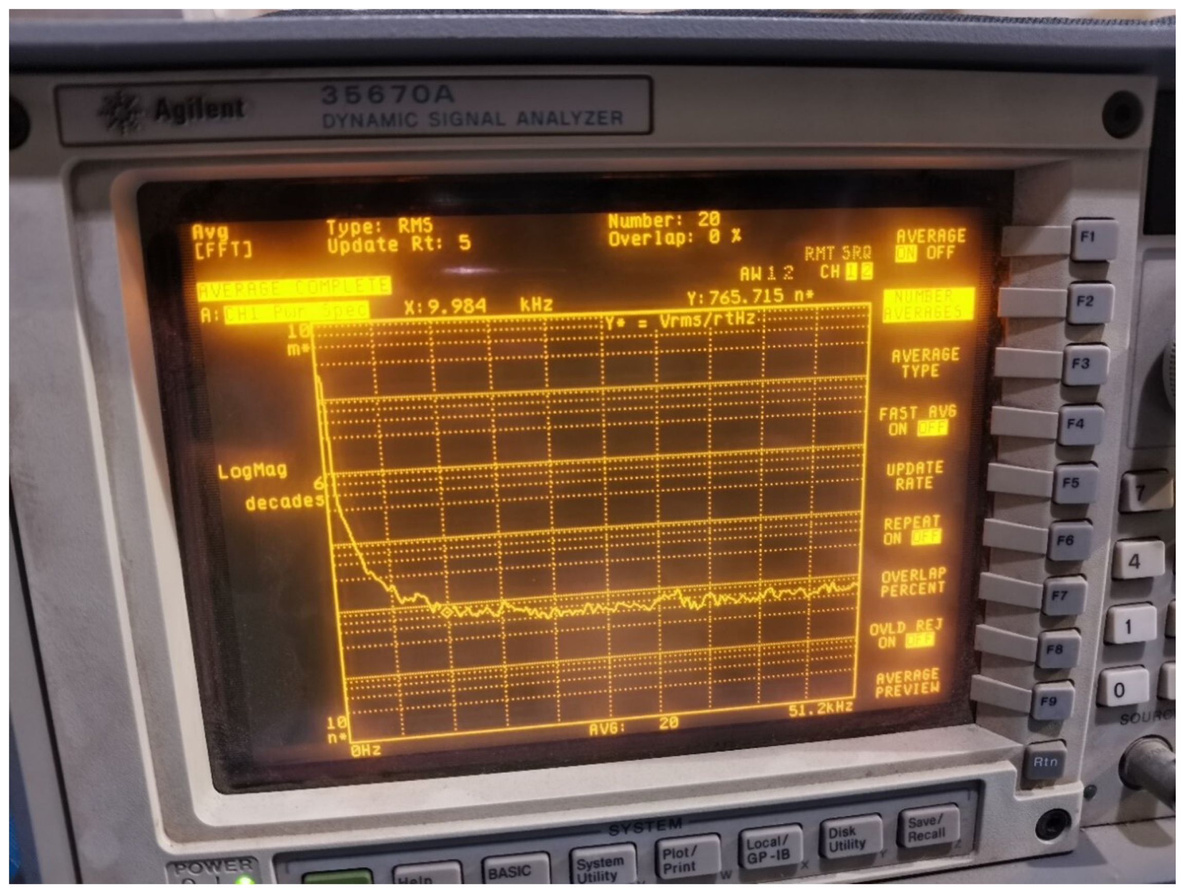
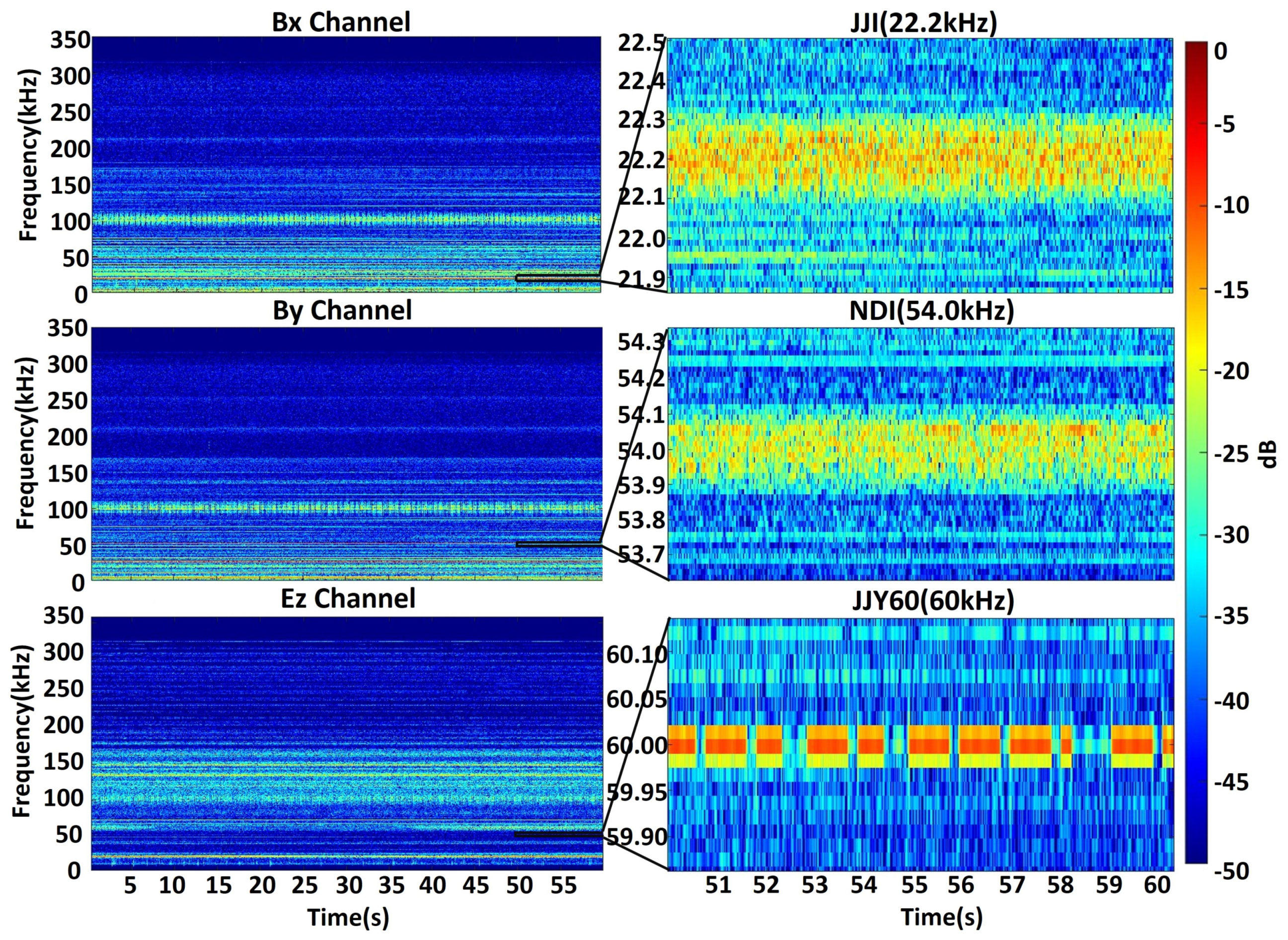
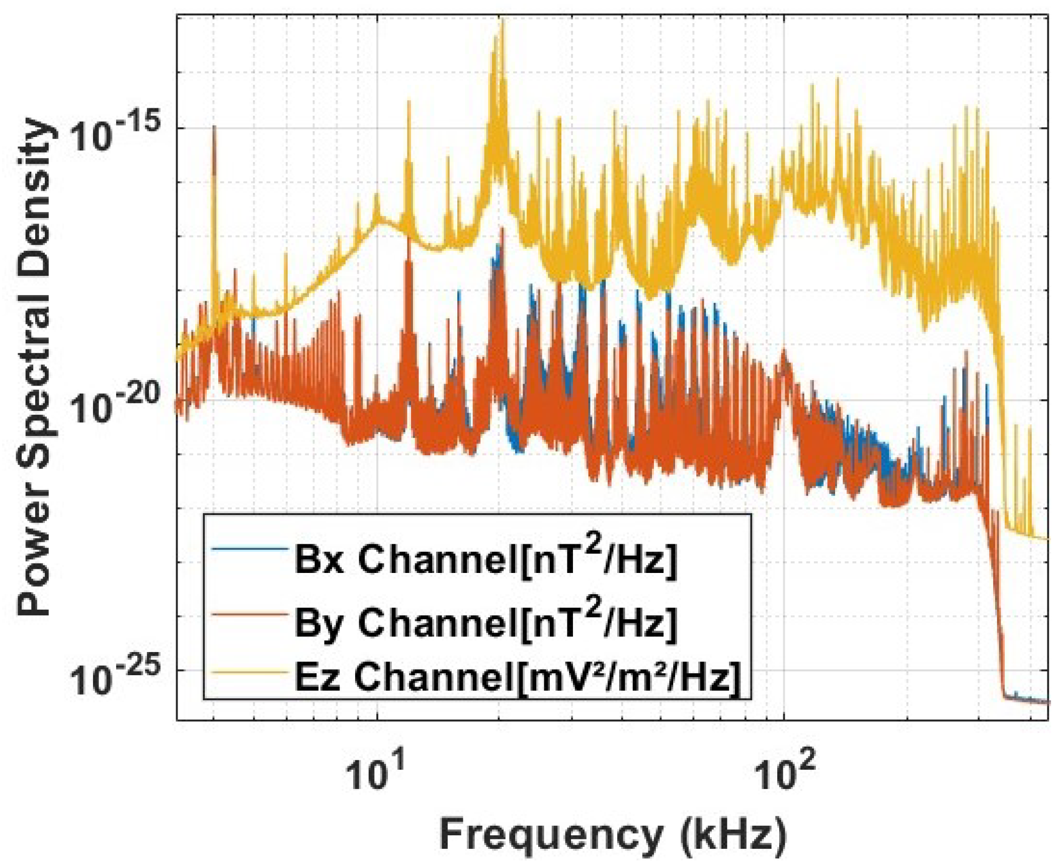
3.1. Measured Wideband Data Analysis

Figure 13 shows the experimental locations of the direction-finding system and the distribution of nearby long-wave stations. The two receivers are arranged in a north–south orientation, with geographic coordinates of 36.37° N, 120.37° E (main) and 36.33° N, 120.37° E (reference). The distance between the receivers is approximately 5.18 km, and their positions nearly overlap on the map. In the figure, the BPC (68.5 kHz) (34.47° N, 115.84° E) transmitter corresponds to the Shangqiu low-frequency time-code broadcasting station [31], NDI (54 kHz) (26.32° N, 127.85° E) is a US Navy submarine communications transmitter station in Okinawa, Japan, and JJI (22.2 kHz) (32.04° N, 130.81° E), also known as the Ebino VLF transmitter (Transmission Station, Ebino Soshinsho), is a transmitter operated by the Japan Maritime Self-Defense Force located in Ebino City, Miyazaki Prefecture, Japan [32]. JJY60 (60 kHz) (33.47° N, 130.18° E) and JJY40 (40 kHz) (37.37° N, 140.85° E) are call signs for low-frequency time signal stations in Japan [33]. Among these, BPC, JJY60, and JJY40 use ASK modulation, while JJI and NDI use MSK modulation [34,35].

Figure 14 displays the time-frequency spectrum of the main receiver’s magnetic and electric antennas for a one-minute. The figure displays amplified time-frequency spectra for the JJI (22.2 kHz), NDI (54 kHz), and JJY60 (60 kHz) frequency bands, focusing on a ten-second segment of data. It is evident that JJI and NDI use MSK modulation, with energy uniformly distributed over time and concentrated within a 200 Hz bandwidth. In contrast, JJY60 uses ASK modulation, with its energy distribution appearing discrete over time.

Figure 15 displays the power spectral density measured by the receiver in Qingdao, Shandong, China. The spectral range from approximately 3 kHz to 300 kHz is primarily dominated by various long-wave radio transmitters (approximately 11 kHz–257 kHz), ocean navigation (LORAN) transmitters (approximately 70 kHz–130 kHz), radio-controlled clocks (approximately 60 kHz–77.5 kHz), and lightning discharges (around 5 kHz–50 kHz) [19].

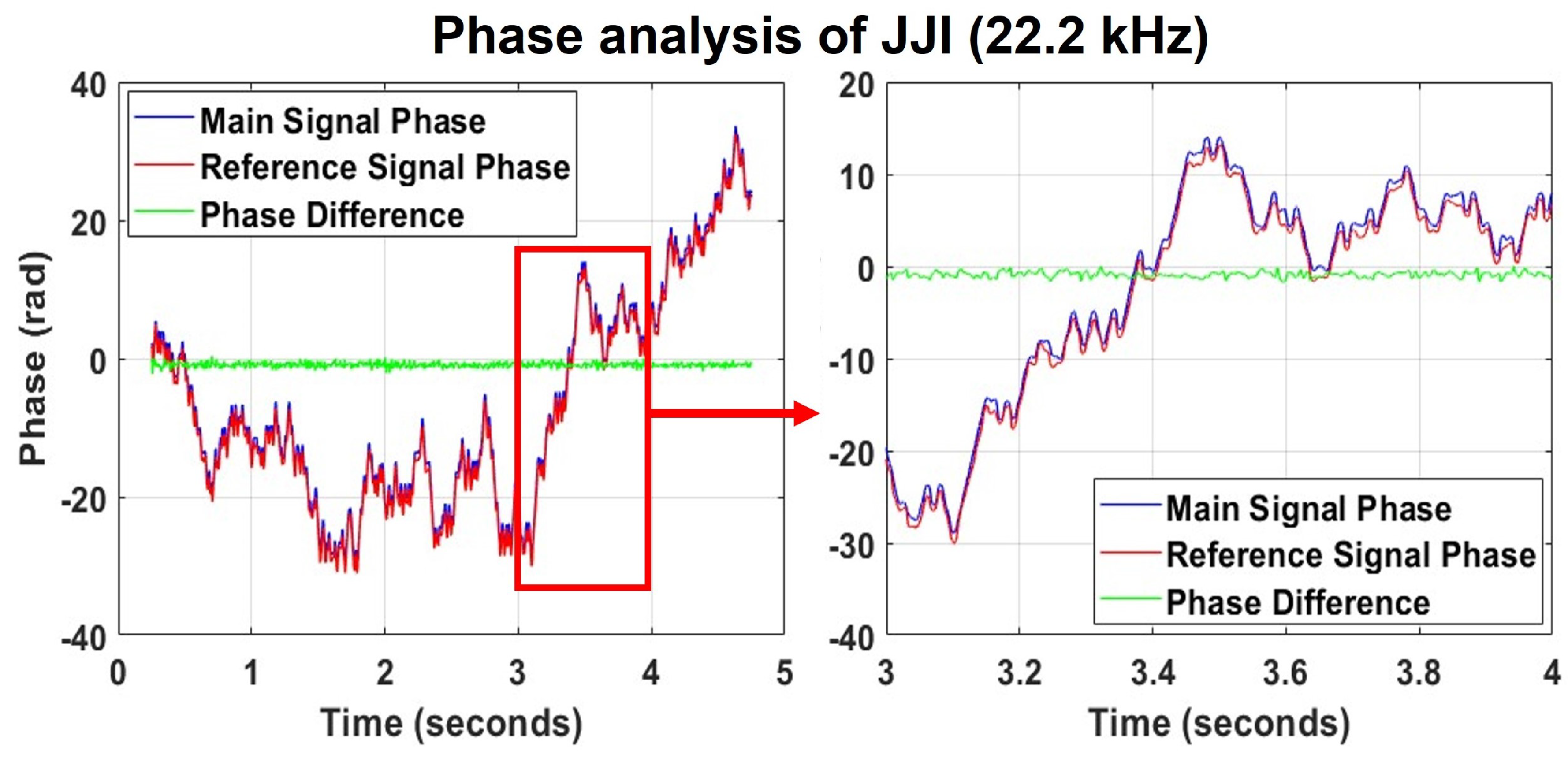
3.2. Narrowband Signal Analysis and Direction Finding

After downconversion and filtering the wideband data to isolate the JJI (22.2 kHz) signal, MSK demodulation was applied. The demodulation results are shown in Figure 16. The three subplots illustrate the relationships between amplitude, frequency, and phase over time between the original signal and the reconstructed demodulated signal. The reconstructed demodulated signal closely matches the original signal, indicating a high degree of fit.

Direction finding was performed on the JJI (22.2 kHz) signal without removing the MSK phase modulation. The phase difference between the two receivers is shown in Figure 17. To avoid filter boundary effects, the data at both ends were truncated. The average phase difference measured over five seconds was −0.90873 radians, resulting in a direction finding result of 112.5624° (due to the two receivers not being strictly aligned north–south, a compensation of +0.42° was applied). The actual azimuth angle was 112.6771°, yielding a direction finding error of 0.1147°. The phase difference introduces minor errors due to MSK modulation; however, averaging over a certain time period can partially mitigate these errors. Experimental results indicate that, without removing the MSK phase modulation, the direction finding results sufficiently meet the requirements. After removing the MSK phase modulation from the same data segment and applying carrier phase direction finding, the result was 112.6596°, with a direction finding error of 0.0175°, improving accuracy.

Direction finding was also performed on the JJY60 (60.0 kHz) signal. Since JJY uses ASK modulation, noise can easily interfere with the signal phase during low-power periods. Furthermore, phase unwrapping introduces phase ambiguities. To obtain stable and reliable results, all stable time segments within a period were extracted, and phase ambiguities were eliminated. The phase analysis results are presented in Figure 18. “Global” refers to the complete segment of raw, unprocessed direction finding data, while “Stable” refers to the phase-stable segment obtained by removing the low-power, phase-unstable segment of the ASK modulation. Within five seconds of data, five phase-stable segments were identified, with an average phase difference of −1.7852 radians. The direction finding result was 106.3202°, compared to the actual azimuth angle of 106.3412°, yielding a direction finding error of 0.0210°.

4. Conclusions

In this study, we designed a compact and highly sensitive long-wave broadband direction-finding system. The system uses two magnetic antennas and one electric antenna, operating over a bandwidth of 10 kHz to 300 kHz. The diameter of the receiving equipment is limited to 45 cm, while maintaining exceptionally high sensitivity. Furthermore, both the magnetic and electric field sensors exhibit flat sensitivity across the device’s operating bandwidth, a feature not found in other devices in existing research. The flat sensitivity across a wide bandwidth ensures that broadband signal waveforms, such as lightning pulses, remain undistorted upon reception, facilitating a more accurate study of their characteristics.

The miniaturization of the equipment enables adaptation to a wider range of application scenarios with minimal site requirements. For direction finding, the system primarily relies on magnetic antennas, supplemented by electric antennas. The use of multiple antennas ensures accurate direction finding of global long-wave radios in various electromagnetic environments, maintaining a maximum direction finding error of less than 2° across a range of angles from 9.9° to 170.1°.

This paper also analyzes the signal characteristics of two modulation modes commonly used in long-wave radios and proposes distinct direction-finding algorithms based on the characteristics of these modulation signals, which have not been discussed in previous studies and provide theoretical support for subsequent long-wave radio direction finding and positioning. The device can serve not only as a precise positioning tool for mobile platforms when GPS is unavailable, but also has potential applications in detecting and localizing lightning pulses and diagnosing ionospheric D-regions.

However, the miniaturization of the device results in a slight reduction in sensitivity, particularly when compared to larger antennas, making it unable to detect extremely weak or distant signals. Future research should focus on optimizing sensor sensitivity, such as by refining the amplifier circuit design for the electrical sensors to achieve a lower noise level.

References

1. Preece, W.H. Earth currents. Nature 1894, 49, 554. [Google Scholar] [CrossRef]
2. Barr, R.; Jones, D.; Rodger, C. ELF and VLF radio waves. J. Atmos. Sol. Terr. Phys. 2000, 62, 1689–1718. [Google Scholar] [CrossRef]
3. Batlló, J. La Radiació ElectromagnèTica: CièNcia, TèCnica, Guerra I Pau. Quad. D’HistÒRia L’Eng. 2004, 6, 331–333. [Google Scholar]
4. Swanson, E. Omega. Proc. IEEE 1983, 71, 1140–1155. [Google Scholar] [CrossRef]
5. Thomson, N. Experimental daytime VLF ionospheric parameters. J. Atmos. Sol. Terr. Phys. 1993, 55, 173–184. [Google Scholar] [CrossRef]
6. Thomson, N.R.; Clilverd, M.A.; McRae, W.M. Nighttime ionospheric D region parameters from VLF phase and amplitude. J. Geophys. Res. Space Phys. 2007, 112, 271. [Google Scholar] [CrossRef]
7. Sechrist, C. Comparisons of techniques for measurement of D-region electron densities. Radio Sci. 1974, 9, 137–149. [Google Scholar] [CrossRef]
8. Kelley, M.C.; Siefring, C.L.; Pfaff, R.F.; Kintner, P.M.; Larsen, M. Electrical measurements in the atmosphere and the ionosphere over an active thunderstorm: 1. Campaign overview and initial ionospheric results. J. Geophys. Res. Space Phys. 1985, 90, 9815–9823. [Google Scholar] [CrossRef]
9. Betz, H.; Schmidt, K.; Oettinger, P.; Wirz, M. Lightning detection with 3-D discrimination of intracloud and cloud-to-ground discharges. Geophys. Res. Lett. 2004, 31, 11. [Google Scholar] [CrossRef]
10. Pessi, A.T.; Businger, S.; Cummins, K.L.; Demetriades, N.W.S.; Murphy, M.; Pifer, B. Development of a Long-Range Lightning Detection Network for the Pacific: Construction, Calibration, and Performance. J. Atmos. Ocean. Technol. 2009, 26, 145–166. [Google Scholar] [CrossRef]
11. Marshall, R.A.; Inan, U.S. Two-dimensional frequency domain modeling of lightning EMP-induced perturbations to VLF transmitter signals. J. Geophys. Res. Space Phys. 2010, 115, 761. [Google Scholar] [CrossRef]
12. Liu, Z.; Koh, K.L.; Mezentsev, A.; Enno, S.; Sugier, J.; Füllekrug, M. Variable phase propagation velocity for long-range lightning location system. Radio Sci. 2016, 51, 1806–1815. [Google Scholar] [CrossRef]
13. Li, J.; Dai, B.; Zhou, J.; Zhang, J.; Zhang, Q. Preliminary Application of Long-Range Lightning Location Network with Equivalent Propagation Velocity in China. Remote. Sens. 2022, 14, 560. [Google Scholar] [CrossRef]
14. Li, J.; Song, L.; Zhang, Q.; Wang, S.; Yang, J.; Ge, Q. Optimizing lightning location accuracy: A study of propagation velocity and time of arrival in long-range lightning location algorithms. Measurement 2024, 234, 114754. [Google Scholar] [CrossRef]
15. Bertoni, F.C.P.; Raulin, J.; Gavilán, H.R.; Kaufmann, P.; Rodriguez, R. Lower ionosphere monitoring by the South America VLF Network (SAVNET): C region occurrence and atmospheric temperature variability. J. Geophys. Res. Space Phys. 2013, 118, 6686–6693. [Google Scholar] [CrossRef]
16. Gross, N.C.; Cohen, M.B.; Said, R.K.; Gołkowski, M. Polarization of Narrowband VLF Transmitter Signals as an Ionospheric Diagnostic. J. Geophys. Res. Space Phys. 2018, 123, 901–917. [Google Scholar] [CrossRef]
17. McCormick, J.C.; Cohen, M.B.; Gross, N.C.; Said, R.K. Spatial and Temporal Ionospheric Monitoring Using Broadband Sferic Measurements. J. Geophys. Res. Space Phys. 2018, 123, 3111–3130. [Google Scholar] [CrossRef]
18. Richardson, D.K.; Cohen, M.B. Seasonal Variation of the D-Region Ionosphere: Very Low Frequency (VLF) and Machine Learning Models. J. Geophys. Res. Space Phys. 2021, 126, e2021JA029689. [Google Scholar] [CrossRef]
19. Füllekrug, M. Wideband digital low-frequency radio receiver. Meas. Sci. Technol. 2010, 21, 015901. [Google Scholar] [CrossRef]
20. Shao, X.M.; Stanley, M.; Regan, A.; Harlin, J.; Pongratz, M.; Stock, M. Total Lightning Observations with the New and Improved Los Alamos Sferic Array (LASA). J. Atmos. Ocean. Technol. 2006, 23, 1273–1288. [Google Scholar] [CrossRef]
21. Wood, T.G.; Inan, U.S. Localization of individual lightning discharges via directional and temporal triangulation of sferic measurements at two distant sites. J. Geophys. Res. Atmos. 2004, 109, 5204. [Google Scholar] [CrossRef]
22. Inan, U.S.; Cohen, M.B.; Said, R.K.; Smith, D.M.; Lopez, L.I. Terrestrial gamma ray flashes and lightning discharges. Geophys. Res. Lett. 2006, 33, 2085. [Google Scholar] [CrossRef]
23. Cohen, M.B.; Said, R.K.; Paschal, E.W.; McCormick, J.C.; Gross, N.C. Broadband longwave radio remote sensing instrumentation. Rev. Sci. Instruments 2018, 89, 094501. [Google Scholar] [CrossRef] [PubMed]
24. Gurses, B.V.; Whitmore, K.T.; Cohen, M.B. Ultra-sensitive broadband “AWESOME” electric field receiver for nanovolt low-frequency signals. Rev. Sci. Instruments 2021, 92, 024704. [Google Scholar] [CrossRef] [PubMed]
25. Cohen, M.; Inan, U.; Paschal, E. Sensitive Broadband ELF/VLF Radio Reception with the AWESOME Instrument. IEEE Trans. Geosci. Remote. Sens. 2010, 48, 3–17. [Google Scholar] [CrossRef]
26. Gurses, B.V.; Whitmore, K.T.; Cohen, M.B. Electric Field Sensor Design for Longwave Radio Reception. In Proceedings of the 2019 SoutheastCon, Huntsville, AL, USA, 11–14 April 2019; pp. 1–2. [Google Scholar] [CrossRef]
27. Krupka, M.A.; Matthews, R.; Say, C.; Hibbs, A.D.; Delory, G.D. Development and Test of Free Space Electric Field Sensors with Microvolt Sensitivity. Nasa Sti/Recon Tech. Rep. 2001, 3, 14007. [Google Scholar]
28. Lu, X.; Chen, L.; Shen, N.; Wang, L.; Jiao, Z.; Chen, R. Decoding PPP corrections from BDS B2b signals using a software-defined receiver: An initial performance evaluation. IEEE Sensors J. 2020, 21, 7871–7883. [Google Scholar] [CrossRef]
29. Yang, Y.; Liu, L.; Li, J.; Yang, Y.; Zhang, T. Featured services and performance of BDS-3. Sci. Bull. 2021, 66, 2135–2143. [Google Scholar] [CrossRef]
30. Dong, D.P.; Wu, H.S.; Guo, Q.F.; Yang, J.W.; Li, X. Research on high-precision time synchronisation technology for sea mobile platforms. Int. J. Inf. Commun. Technol. 2024, 24, 57–70. [Google Scholar] [CrossRef]
31. Feng, P.; Wu, G.; Bai, Y.; Ding, X. Additional spread spectrum modulation timing method in BPC. In Proceedings of the Sixth International Symposium on Precision Engineering Measurements and Instrumentation, Hangzhou, China, 8–10 August 2010; Volume 7544, pp. 500–505. [Google Scholar] [CrossRef]
32. Wu, C.; Qiu, S.; Wang, N.; Denisov, O.; Qiu, J.; Molebny, V. A Simple Analysis of The Development and Future of Long-wave Transmitting Antenna. In Proceedings of the 2023 6th International Conference on Electronics Technology (ICET), Chengdu, China, 12–15 May 2023; pp. 277–281. [Google Scholar] [CrossRef]
33. Basak, T.; Hobara, Y.; Pal, S.; Nakamura, T.; Izutsu, J.; Minatohara, T. Modeling of Solar Eclipse effects on the sub-ionospheric VLF/LF signals observed by multiple stations over Japan. Adv. Space Res. 2024, 73, 736–746. [Google Scholar] [CrossRef]
34. Yamazaki, S.; Onishi, K.; Goto, T.n.; Mikada, H.; Konishi, N. Feasibility study of subsurface electromagnetic exploration using longwave radio-clock time-signal. In Proceedings of the 9th SEGJ International Symposium. Society of Exploration Geophysicists of Japan, Sapporo, Japan, 12–14 October 2009; pp. 1–4. [Google Scholar] [CrossRef]
35. Ohya, H.; Suzuki, T.; Tsuchiya, F.; Nakata, H.; Shiokawa, K. Variation in the reflection height of VLF/LF transmitter signals in the D-region ionosphere and the possible source: A 2018 meteoroid in Hokkaido, Japan. Radio Sci. 2024, 59, 1–10. [Google Scholar] [CrossRef]
Figure 1. Information flow diagram of the long-wave wideband direction-finding system.
Applsci 15 02570 g001
Figure 2. Schematic of the E-field and B-field sensors.
Applsci 15 02570 g002
Figure 3. Equivalent circuit diagram of the flux feedback type broadband inductive magnetic field sensor.
Applsci 15 02570 g003
Figure 4. Conversion factor of the inductive magnetic field sensor.
Applsci 15 02570 g004
Figure 5. Schematic diagram of the electric field sensor working principle.
Applsci 15 02570 g005
Figure 6. Schematic of parallel-plate capacitor and low-noise amplifier circuit.
Applsci 15 02570 g006
Figure 7. Equivalent noise level of the sensor.
Applsci 15 02570 g007
Figure 8. Magnetic field antenna noise test results: 765 nV at 10 kHz, with a conversion factor of 100 mV/nT, corresponding to a noise level of 7.65 f T / Hz .
Applsci 15 02570 g008
Figure 9. Electric field antenna noise test results: 3.2 μ V at 10 kHz, with a conversion factor of 1 V/m, corresponding to a noise level of 3.2 μ V / m Hz .
Applsci 15 02570 g009
Figure 10. Time-frequency transmission principle diagram of Beidou co-viewing.
Applsci 15 02570 g010
Figure 11. Schematic diagram of the one-dimensional interferometric measurement principle.
Applsci 15 02570 g011
Figure 12. Distribution of direction finding error σ α with incident angle α .
Applsci 15 02570 g012
Figure 13. Position distribution of transmitter and receiver and electromagnetic propagation path.
Applsci 15 02570 g013
Figure 14. Time-frequency spectrum of three channels within one minute.
Applsci 15 02570 g014
Figure 15. Power spectral density of three antennas of the main receiver within one minute.
Applsci 15 02570 g015
Figure 16. MSK demodulation results of the main receiver for the JJI (22.2 kHz) signal.
Applsci 15 02570 g016
Figure 17. Phase analysis of signals from main and reference receivers within five seconds in the JJI (22.2 kHz) signal bandwidth.
Applsci 15 02570 g017
Figure 18. Phase analysis of signals from main and reference receivers within five seconds in the JJY60 (60.0 kHz) signal bandwidth.
Applsci 15 02570 g018