Local Balance and Information Aggregation: A Method for Identifying Central Influencers in Networks

Abstract

In complex networks, identifying critical nodes plays an important role in information dissemination. Due to the dual property of nodes to both propagate and receive information, information is propagated repeatedly in a restricted area where critical nodes are closely connected, making it impossible to accurately identify key nodes. In this paper, we propose a new method for identifying critical nodes—LBIA (local balance and information aggregation). The method first defines a metric named “local balance” as the propagation information, and also proposes an algorithm that combines the probability and k-shell (PKs) to encapsulate the node’s individual information. Subsequently, by simulating the dissemination of information in the real world, the propagation information is aggregated with the node’s individual information to accurately identify key nodes. The Kendall and Jaccard coefficients measure the consistency of node ranking results with SIR results, as well as the number of matching nodes, while monotonicity evaluates the algorithm’s capacity to distinguish nodes and prevent identical values for distinct nodes. Experiments conducted on both densely interconnected networks and general networks reveal that LBIA achieves an average Kendall value of 0.7330, a Jaccard coefficient ranging from 0.6 to 0.8, and a monotonicity of 1. These results highlight LBIA’s precision in identifying key nodes and its robust applicability across diverse network structures.

1. Introduction

In complex networks, nodes play different roles and have different functions. A small number of nodes possess the capability to exert a substantial influence on the structure and functionality of the network. The identification of influential nodes is crucial for ensuring network stability and facilitating efficient information dissemination [1]. Evaluating and ranking the influence of nodes is a vital aspect of research in spreading dynamics. This approach helps locate influential nodes in complex networks, enhancing the understanding and control of propagation processes within the networks [2], such as in biological sciences [3], management sciences [4], computer sciences [5], and intrusion detection [6], among others. Besides its theoretical significance, it has practical applications as well. For example, in disease control [7], the key issue in accelerating or controlling the spread of epidemics in complex networks is to choose an appropriate set of initial spreaders (or immunization nodes) [8], where the spread of disease can be effectively stopped by tracking and managing key persons. A similar function is used in tracking public opinion [9,10] and rumor detection [11]. In terrorist and insurgent networks [12], terrorist network service communication channels are disabled by strategically removing critical nodes. In transportation networks [13], the paralysis of critical nodes can have significant impacts on the connectivity, access efficiency, and capacity allocation of the entire transportation network.

Existing algorithms can be categorized into local, semi-local, and global algorithms based on the characteristics of the nodes in the network. Lü et al. proposed an algorithm named Weight LeaderRank [14], which assigns degree-related weights to links associated with nodes. This algorithm outperforms the PageRank [15] algorithm in identifying important nodes, is more tolerant of noisy data, and is more robust against attacks. Guiqiong Xu et al. proposed a local propagation probability (LPP) [16] model to identify key nodes by recursively calculating the local propagation probability of each node, respectively seeking the propagation influence score between neighboring nodes of the same and different orders, and separating the nodes layer by layer based on the hierarchical structure score of the nodes. Jie Zhao et al. measure the global importance of each node (GIN) [17], considering the influence of the node itself and its neighbors, which enables a more accurate identification. The k-shell algorithm identifies important nodes by decomposing the network layer by layer to examine their relative positions. However, it suffers from coarse granularity in identification. Local algorithms have a low time complexity but limited granularity, whereas global algorithms achieve higher accuracy at the cost of computational efficiency. Consequently, semi-local algorithms are often the superior choice.

Due to the property of nodes to both propagate and receive information, information is repeatedly propagated in restricted areas where nodes are closely connected. Based on this, this paper proposes a semi-local algorithm called LBIA, which accurately identifies key nodes in the restricted region while maintaining a low time complexity. The main contributions of LBIA are outlined below.

Contributions

In this paper, we propose a new method for identifying critical nodes—LBIA. This algorithm solves the problem of the rough identification strength in the k-shell algorithm, and it can accurately identify important nodes in the restricted area. It has a low time complexity as it only considers information from neighbors. Through experiments on both densely interconnected networks and general networks, the average Kendall coefficient value is 0.7330, the Jaccard coefficient value is 0.6 to 0.8, and the monotonicity value is 1. The recognition ability is more advantageous compared to the comparison algorithms, while it is suitable for most network types.

The rest of this paper is organized as follows. Section 2 provides an overview of related work, including traditional classical algorithms and recently proposed advanced algorithms. Section 3 introduces key definitions, the SIR model used in this paper, and the k-shell algorithm. Section 4 presents the PKs algorithm and $L{B}_v$, describes the core idea of the LBIA algorithm, and provides concrete examples to facilitate understanding. Section 5 details the experimental setup, dataset, and evaluation metrics, followed by extensive comparative experiments for analysis and discussion. Finally, Section 6 provides conclusions and a vision for future work.

2. Related Work

The node centrality method is typically used to measure the influence of a node’s relative position in a network. These algorithms provide an intuitive way to assess node importance. Degree centrality (DC) [18] determines a node’s importance by directly counting the number of neighbors of the node. However, it is not able to distinguish the relative importance between nodes with the same number of neighbors. Closeness centrality (CC) measures the average distance of a node from all other nodes in the network, favoring more centrally located nodes. While this approach provides a global perspective, it also has high time complexity. Betweenness centrality (BC) [19] quantifies the frequency with which a node appears in the shortest paths between pairs of other nodes. A higher betweenness centrality value indicates that a node is more likely to serve as a crucial mediator in information flow. Similar to closeness centrality, BC also suffers from high time complexity.

In recent years, several advanced algorithms have been proposed to identify key nodes in networks. The Local Clustering H-index (LCH) [20] incorporates neighborhood topology, node degree, and node quality, integrating local network characteristics with the clustering coefficient’s influence, thereby enhancing the accuracy of key node identification. Zareie et al. introduced the Extended Cluster Coefficient Ranking Measure (ECRM) [21], which refines node identification by incorporating hierarchical structures and layering the network at a finer granularity. Chen and Lü [22] proposed a semi-local centrality measure as a trade-off between low-correlation centrality and computationally expensive metrics, significantly reducing computational complexity. Hajarathaiah et al. developed the Nearest Neighborhood Trust PageRank (NTPR) [23], which leverages structural attributes of both neighbors and nearest neighbors. This method defines ranking metrics based on degree ratio, node similarity, and the trust values of neighboring nodes. Ramya et al. extended this idea by collecting information from multiple levels of neighborhoods, introducing the Global Structural Influence (GSI) [24] method, which considers both local and global influences within the network.

In addition to these algorithmic improvements, some researchers have combined existing algorithms with a variety of fields. Yang et al. combined the k-shell algorithm with the gravitational formulation from physics, proposing an improved gravity centrality measure called KSGC [25]. This approach refines gravitational centrality by considering node positions in advance, thereby improving identification accuracy. Zhou et al. [26] proposed the PW algorithm, which utilizes the eigenvectors of the maximum and minimum eigenvalues of the Laplacian matrix to identify optimal nodes for optimizing the coupling range, and to control or influence the overall network behavior by ‘pinning’ these nodes. Sun et al. proposed the IDME (Information Diffusion and Matthew Effect Aggregation) [27] method by using the Matthew effect to aggregate information from multiple neighboring layers.

Existing algorithms typically identify critical nodes by evaluating node characteristics and network topology. The LBIA algorithm builds upon this framework by incorporating the dynamic properties of information propagation, considering both the information reception and dissemination capabilities of nodes to achieve the more accurate identification of critical nodes. This approach effectively integrates the high resolution of global algorithms with the computational efficiency inherent in local algorithms, thereby offering a more refined and efficient solution for critical node identification.

3. Background

In this section, we will introduce some basic definitions used to characterize the tightness of connections between nodes. Next, we analyze the specific process of the k-shell algorithm to identify its limitations and propose improvements. Finally, we introduce the SIR propagation model used in this paper.

3.1. Definition

Consider a given complex network $G=(V,E)$, where V represents the set of vertices and E represents the set of edges. Furthermore, denote the number of vertices and edges as $\left|V\right|$ and $\left|E\right|$. The node degree and clustering coefficient can be used to describe the degree of connection between nodes. The Jaccard coefficient can measure the number of common neighbors between two nodes. By formalizing these basic definitions, the LBIA algorithm can be explained more concisely and accurately.

Definition 1

(Node Degree [18]). The degree of a node is the number of edges connected to it. It serves as a important metric for describing network connectivity. It is often used to measure the centrality and importance of a node within the network; where d represents the degree of a node in the undirected network G and is shown in Equation (1):

$$d_x=\sum _{j=1}^N{a}_{xj}$$

(1)

Definition 2

(Clustering Coefficient [28]). The clustering coefficient mainly determines whether a node is tightly connected or not by the ratio of the number of connecting edges that actually exist between the neighbors of the node to the number that theoretically exist. It is shown in Equation (2):

$$C_x={\displaystyle \frac{2\ast m_x}{d_x\ast (d_x-1)}}$$

(2)

Definition 3

(Jaccard Coefficient [29]). In a graph, the Jaccard coefficient is used to describe the number of common neighbors between two nodes, the larger the coefficient, the more connected the nodes are. It is shown in Equation (3):

$$J_{xy}={\displaystyle \frac{|{\varphi }_x\cap {\varphi }_y|}{|{\varphi }_x\cup {\varphi }_y|}}$$

(3)

where ${\varphi }_x$ represents the first-order neighbor set of node x and ${\varphi }_y$ represents the first-order neighbor set of node y. Here, we add the node itself to the set of neighbors.

3.2. k-Shell Algorithm

The k-shell decomposition algorithm (ks) [30] is a classical and efficient algorithm for measuring the node influence in networks based on node position information. Moving from the outermost layer to the innermost layer, the relative importance of nodes increases. 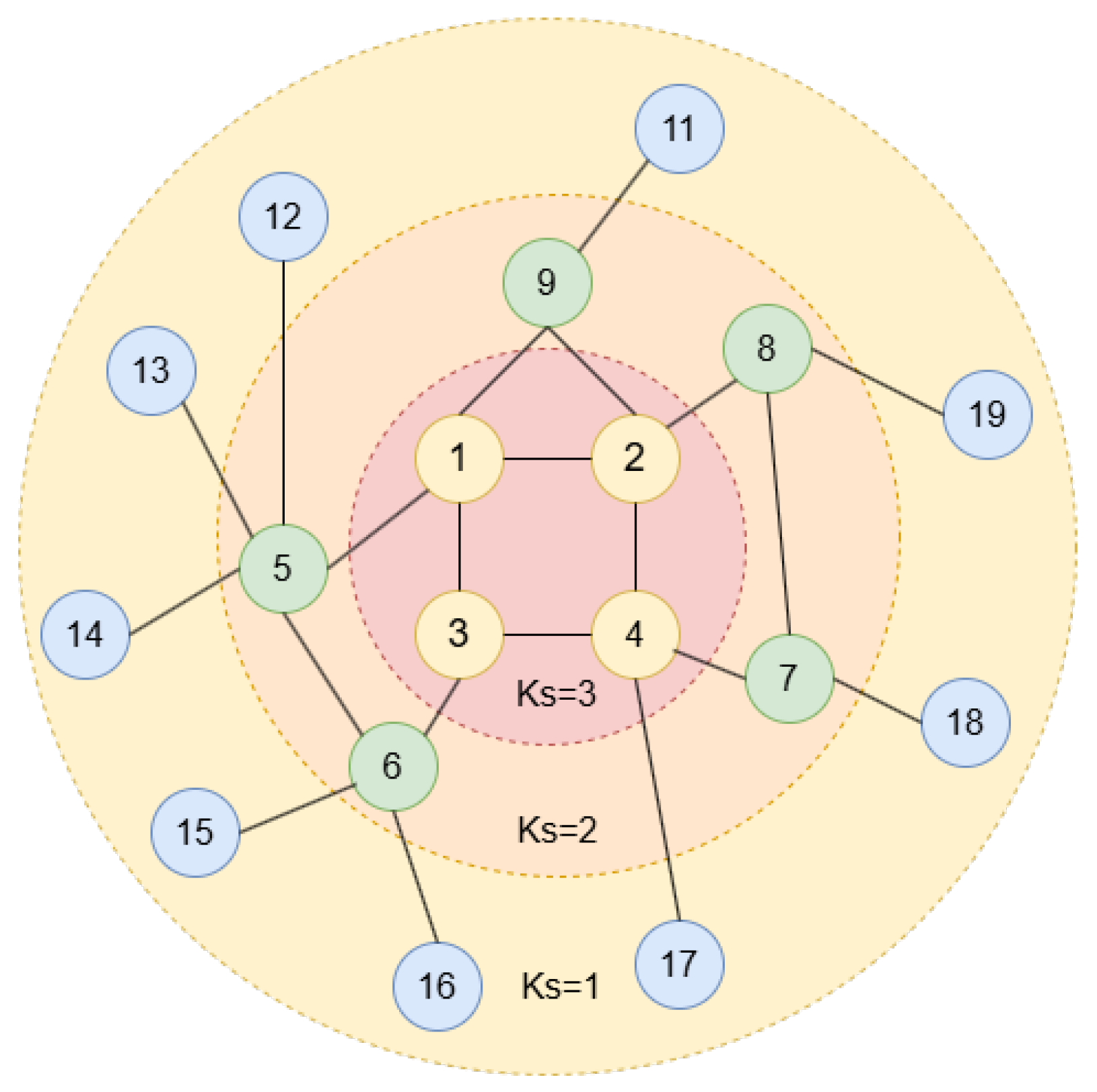One advantage of this method is its low computational complexity; however, the k-core decomposition process does not consider the topological position of nodes, leading to poor node identification [31]. The steps are as follows:

• First, remove all isolated nodes from the network. Then, all the nodes in the network whose degree value is 1 are noted as $k_s=1$, and then remove these nodes from the network with their connected edges to obtain a new network. Consecutively perform the same steps until there are no nodes whose degree value is 1 in the network;
• After, mark all the nodes in the network whose degree value is 2 as $k_s=2$, and then remove these nodes with connected edges from the network similarly, repeating the steps until all nodes with a degree value of 2 are removed;
• Continue repeating the above steps. After each operation, the degree value is increased by 1, and the $k_s$ value is also increased by 1, until all the nodes in the network are deleted. At this point, all nodes’ $k_s$ values are obtained, which better describes the hierarchical structure of the nodes in the network.

The decomposition process is shown in Figure 1. Nodes in higher layers are more important; however, the importance among multiple nodes in the same layer cannot be judged.

3.3. SIR Model

The SIR model is an epidemiological model used to describe the spread of infectious diseases in a population [32] and has been a foundational model in epidemiology for nearly a century. It illustrates fundamental trade-offs and provides a simple framework that can be easily built on. Subsequent work in epidemiological theory has extended the model in various ways, and modern epidemiological forecasts typically work with variants that are more flexible in a number of dimensions [33]. The SIR model divides the population into three categories: Susceptible—this group is not immune and can be infected; Infected—this group is already infected with the disease and can spread it to susceptible people; Recovered—this population has recovered and gained immunity and is no longer infected or transmitting the disease. The modeled transmission process can be described by Equation (4):

$$\left\{\begin{array}{c}{\displaystyle \frac{dS}{dt}=-\beta \ast S\ast I}\hfill \\ {\displaystyle \frac{dI}{dt}=\beta \ast S\ast I-\gamma }\hfill \\ {\displaystyle \frac{dR}{dt}=\gamma \ast I}\hfill \end{array}\right.$$

(4)

where S represents the number of susceptible persons, I represents the number of infected persons, R represents the number of recovered persons, $\gamma$ is the immunization rate, indicating the number of recovered persons per unit time, and $\beta$ is the infection rate, indicating the number of infected persons that can transmit to susceptible persons per unit time.

The propagation process of the SIR model is as follows: A node is initially designated as the source node and set to the infected state. During the first infection, its neighboring nodes are randomly infected based on a given propagation probability. After the infection is completed, the source node is set as a recovered node. At this point, newly infected nodes continue to spread the infection in subsequent rounds until only susceptible and recovered nodes remain in the network.

4. The Proposed Method

This paper introduces a critical node identification algorithm named LBIA, which represents a novel method to accurately identifying important nodes in complex networks by integrating local balance and information aggregation. The information primarily consists of two components: the PKs algorithm solves the problem of the rough identification strength in the k-shell algorithm while encapsulating the individual information of nodes. $L{B}_v$ can solve the problem of bias in the recognition of nodes in the restricted area while encapsulating propagation information between nodes. Subsequently, the LBIA algorithm aggregates the propagation information with the individual information of the nodes to accurately identify the important nodes. In this section, the PKs algorithm, $L{B}_v$ and LBIA algorithm are introduced.

4.1. PKs (Probability and k-Shell)

During propagation, changes in the probability of propagation affect the extent to which a node can propagate. This is because a lower probability of propagation puts the entire network in a state of complete immunity before it is fully propagated. Therefore, changes in the propagation probability can have a significant impact on node identification. The k-shell algorithm has the disadvantage that the nodes in the same layer cannot recognize the cruciality, and the recognition granularity is coarse. The influence level of nodes in the network changes with the propagation probability, which means that the ranking of nodes by their influence level will also change accordingly. Based on this, this paper proposes the PKs (probability and k-shell) algorithm, which combines the propagation probability with the k-shell algorithm, thereby addressing the issue of coarse recognition strength.

For a particular node, when the propagation probability is low, greater consideration should be given to the number of nodes with higher influence levels in its immediate neighbors. Conversely, when the propagation probability is high, more emphasis should be placed on the number of nodes with higher influence levels in its distant neighbors. Then, the value $P{K}_s$ for node i is shown in Equation (5):

$$P{K}_s\left(i\right)=({\beta }_{max}-\beta )\ast k_s\left(i\right)+\beta \ast \sum _{j\in N\left(i\right)}{k}_s\left(j\right)$$

(5)

where ${\beta }_{max}$ is the maximum propagation probability, $\beta$ is the current propagation probability, $k_s\left(i\right)$ is the k-shell value of node i, and N(i) is the first-order neighbor set of node i.

4.2. Local Balance Value

In complex networks, during a propagation process, since nodes can both transmit and receive information, when nodes in a region are too closely connected to each other, the information will be propagated repeatedly in that region, which may lead to bias in the process of identifying critical nodes.

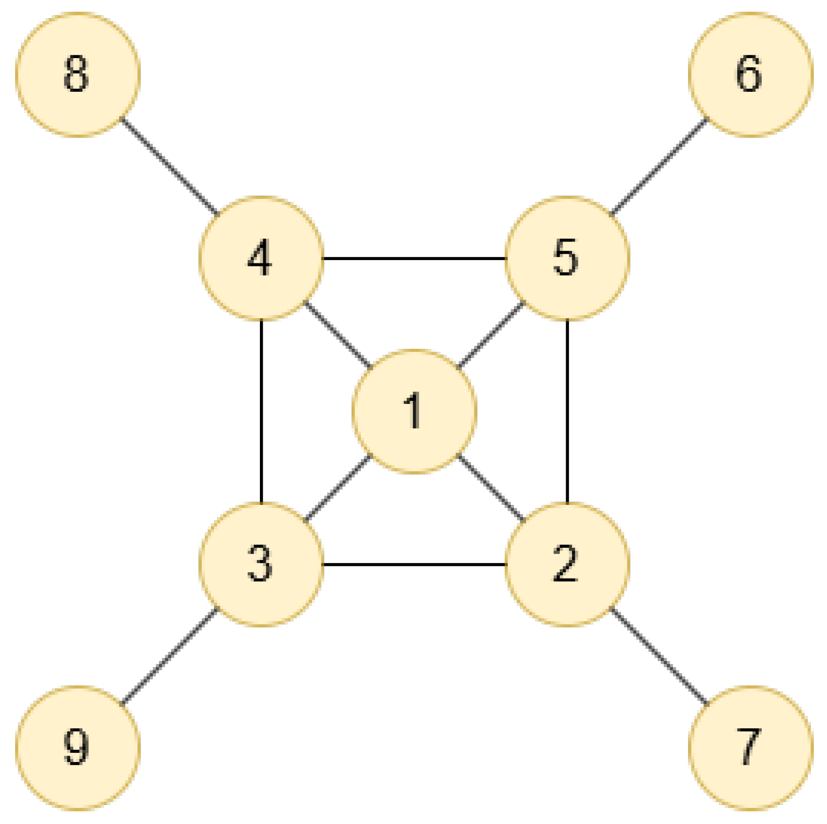
For example, as shown in Figure 2, assuming the initial information value of each node is 1 and taking node 1 as an example, the information from its first- and second-order neighbors is aggregated. The information value of node 2 becomes 4 after aggregating its first-order neighbors. Similarly, the aggregated information values of the remaining first-order neighbors are computed. Finally, by aggregating the information of nodes 2, 3, 4, and 5 along with its own information, the result is 17. Similarly, the final information values of nodes 2, 3, 4, and 5 are calculated as 13. However, when node 1 is removed, information can still propagate between the remaining nodes, maintaining the overall connectivity of the network. If node 2 is removed, however, information cannot propagate from the main part of the network to node 7, and similar situations occur when nodes 3, 4, or 5 are removed. Therefore, from the perspective of overall network connectivity and information propagation, the contribution of node 1 to information diffusion is relatively low, while the role of node 2 becomes significantly more important.

This indicates that the importance of a node depends on the number of its direct neighbors as well as the number of actual connected edges. The clustering coefficient in the network is used to describe the actual connection between the nodes. When the clustering coefficient is 1, it means that there are connecting edges between all the nodes in the region formed by the node and its neighboring nodes; so, the higher the clustering coefficient of a node, the more the information has been re-propagated, the higher the degree of a node, and the more nodes it can transmit information to. To balance the importance of the nodes and make them more representative, we comprehensively considered the clustering coefficient and degree value of each node in the network, and propose the concept of the local balance value $\left(L{B}_v\right)$, as shown in Equation (6):

$$L{B}_v\left(i\right)={\displaystyle \frac{d_i-1}{c_i+{\sum }_{j\in N\left(i\right)}{c}_j+1}}$$

(6)

where $d_i$ is the degree of node i, $c_i$ is the clustering coefficient of node i, and N(i) is the first-order neighbor set of node i. This value can effectively address the issue of bias in assessing node importance.

Through the calculation of Equation (6), $L{B}_v=1$, $L{B}_v(2,3,4,5)=9/8$, and $L{B}_v(6,7,8,9)=0$. The results show that node 6, 7, 8, and 9 are in marginal positions and are, therefore, less important. $L{B}_v\left(1\right)$ is lower than $L{B}_v(2,3,4,5)$. Thus, the local balance value can accurately identify critical nodes within the restricted area.

4.3. LBIA Algorithm

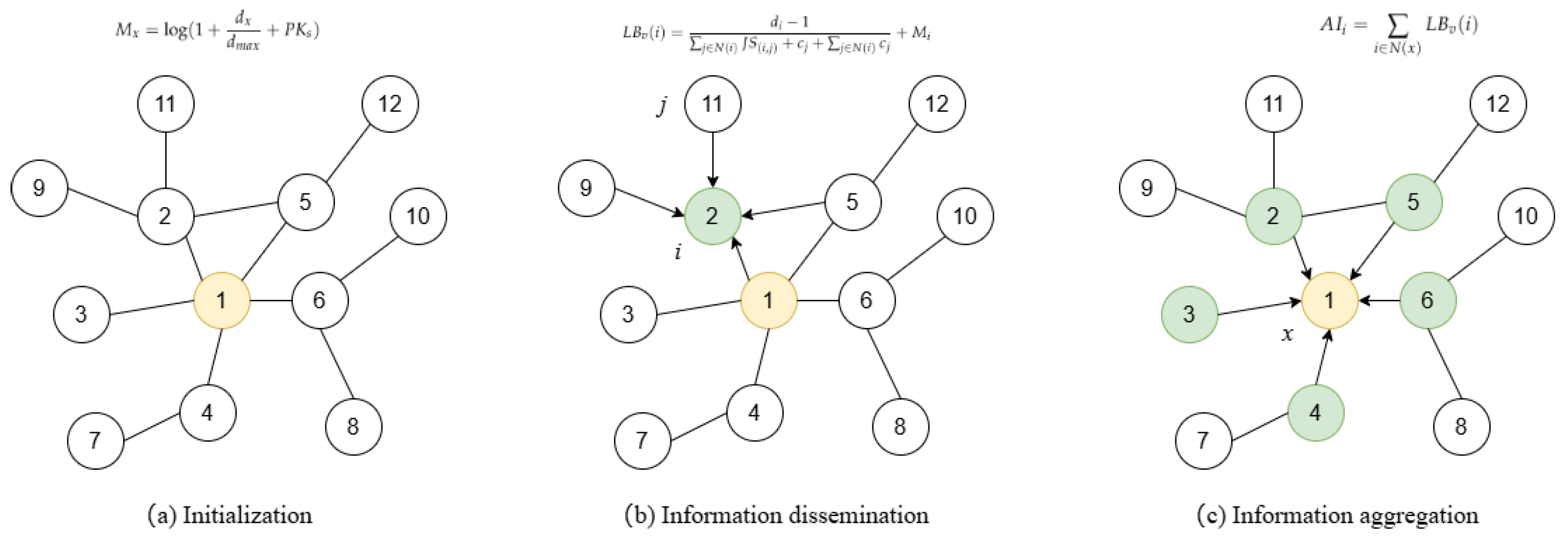
In this section, we will describe the proposed algorithm. Figure 3 shows the procedures of information dissemination and information aggregation between nodes in the toy network.

4.3.1. Algorithm Process

The algorithm process is as follows:

• Assign initial information to each node in the network. The initial information $M_x$ for each source node x in the LBIA algorithm is defined as shown in Equation (7):

  $$M_x=log(1+{\displaystyle \frac{d_x}{d_{max}}}+P{K}_s)$$

  (7)
• Select a node and calculate the information propagated by all its neighboring nodes. The propagation information $L{B}_v$ from node j to node i is defined as shown in Equation (8):

  $$L{B}_v\left(i\right)={\displaystyle \frac{d_i-1}{{\sum }_{j\in N\left(i\right)}J{S}_{(i,j)}+c_j+{\sum }_{j\in N\left(i\right)}{c}_j}}+M_i$$

  (8)

  where $M_i$ represents the initial information of node i, $J{S}_{(i,j)}$ represents the Jaccard coefficient between node i and node j, $c_i$ represents the clustering coefficient of node i, and N(i) is the first-order neighbor set of node i;
• Aggregate the propagated information from all neighboring nodes, and the aggregation information (AI) of node i is defined as shown in Equation (9):

  $$A{I}_i=\sum _{i\in N\left(x\right)}L{B}_v\left(i\right)$$

  (9)
• Considering both the node’s own information and the aggregation information from its neighbors. The final value LBIA is defined as shown in Equation (10):

  $$LBI{A}_x=L{B}_v\left(x\right)+A{I}_i$$

  (10)
• Finally, repeat steps II, III, and IV to calculate the LBIA values for all nodes in the network.

4.3.2. The Details of the Algorithm

In the first step, degree normalization and PKs are used to calculate the initial information of each node. The propagation ability is considered to be proportional to its degree value and positional information. The degree of a node can reflects its ability to disseminate information; the larger the degree value, the more paths the information may choose. PKs represents an optimized measure of the node’s position. There is an area of the network consisting of multiple important nodes, which belongs to the core of the network, and nodes in the state of the core are more efficient at propagating information.

In a network, information propagation between nodes is achieved through connections and interactions between nodes. Information propagates from the source node through the network, first to the surrounding nodes and then outward. This propagation usually creates a wave propagation effect in the network, gradually affecting more nodes, and each node receives information from its neighbors. The Jaccard similarity can describe the common information between two nodes. The higher the similarity, the higher the number of common neighbors between the nodes; therefore, the information dissemination will also be limited to a small area. By comprehensively considering the Jaccard coefficient, we extend the previously mentioned local balance value (Equation (5)) as the information propagated between nodes.

4.4. Example Analysis

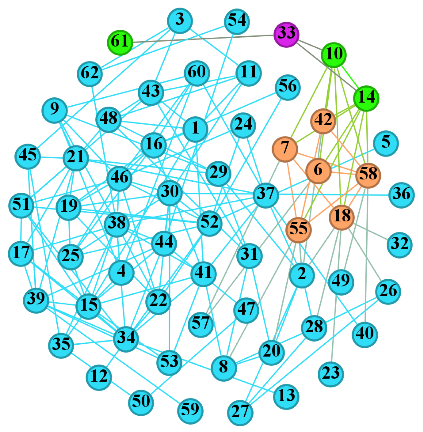
The higher the average clustering coefficient of the network, the more connected edges exist between nodes in the network, and the more closely connected they are. Due to the ease of visualization of the Dolphins network as well as its high average clustering coefficient, in this section, the Dolphins network is taken as an example to introduce the computation process of the LBIA algorithm. Figure 4 depicts the Dolphins network, which includes 62 nodes and 159 edges. Node 33 was selected as the source node, and its first- and second-order neighbors were generated, where purple indicates the source nodes, green is the first-order neighbor node, and orange is the second-order neighbor node.

First, the information value of the source node 33 was calculated according to Equation (7):

$$M\left(33\right)=log(1+3/12+0.42)\approx 0.58$$

Next, we took the first-order neighbor node 10 as an example:

$$L{B}_v\left(10\right)\approx {\displaystyle \frac{6}{3.58+0.52+3.05}}+1.93\approx 2.76$$

Then, $L{B}_v\left(14\right)\approx 2.90$, $L{B}_v\left(61\right)\approx 0.33$, which were summed to obtain $A{I}_{33}\approx 6$, and the final result is $LBI{A}_{33}\approx 7.91$ using Equation (10). Similarly, we found the impact value of the other nodes, and arranged all the nodes in descending order according to their impact values, thereby obtaining a ranked list of the nodes, where a higher rank indicates that the node occupies a more important position in the network.

5. Experiment

5.1. Experimental Setup

To evaluate the performance of LBIA, we compared it with eight representative critical node identification algorithms: betweenness centrality (BC) [19], cluster centrality (CC), degree centrality (DC) [18], PageRank [15], KSGC [25], LCH [20], NTPR [23], and IDME [27]. These algorithms cover segmentation by centrality, improvements to classical algorithms, and algorithms that analyze the network structure in terms of its structure. It is more convincing to compare LBIA with algorithms identified from these different perspectives. For the scientific validity of the results, experiments were conducted on the accuracy of different algorithms in terms of recognition ability.

In various diffusion networks, infectious disease models such as SIR are utilized to detect critical nodes [34]. A low propagation probability will result in the under-propagated of information, while a high propagation probability will lead to rapid propagation in a short period, which is of no research significance. In order not to lose generality, the propagation probability was set to 0.1. When the recovery probability was set to 1, the infected nodes were immune in the next round, which effectively reduced the time required by the algorithm. Since there may be situations where no node is infected during the first propagation, we ran 1000 iterations of the SIR model to obtain the average propagation value of the nodes.

5.2. Dataset

The higher the density of connections within regions of a network, the greater its average clustering coefficient. To enhance the generalizability of the experiment, the networks analyzed were categorized into two distinct types: the tightly interconnected networks—USAir97, Bio-celegans, Soc-hamster, CA-GrQc; and the general networks—Dolphins, Eurroad, Rt-assad, CiteSeer, CA-Erdos992. These datasets can be found at https://networkrepository.com/index.php (accessed on 20 October 2024), and their structural features are shown in

Table 1. Real network dataset.

DataSet	n	e	$\langle \mathit{k}\rangle$	$\langle \mathit{AC}\rangle$	${\mathit{d}}_{\mathit{m}\mathit{a}\mathit{x}}$
Dolphins	62	159	5.13	0.25	12
USAir97	332	2126	12.80	0.75	139
Bio-celegans	453	2025	8.95	0.65	237
Eurroad	1174	1417	2.41	0.02	10
Rt-assad	2139	2788	2.00	0.02	152
Soc-hamster	2426	16,630	13.71	0.54	273
CiteSeer	3264	4536	2.80	0.24	99
CA-GrQc	5242	14,496	5.53	0.53	81
CA-Erdos992	6100	7515	2.95	0.28	61

, where n is the number of nodes, e is the number of edges, $\langle k\rangle$ denotes the average degree, $\langle AC\rangle$ denotes the average clustering coefficient, and $d_{max}$ is the maximum degree in the network.

5.3. Evaluation Index

To assess the performance of each comparison method from different perspectives, we utilized three widely recognized metrics to evaluate the effectiveness of key node identification.

5.3.1. Kendall Coefficient

The Kendall coefficient [35] is also known as the Kendall rank correlation coefficient. It is a statistical index that measures the sequential correlation of two random variables. It measures whether two variables are in the same order. The value range is usually between −1 and 1, where:

• A Kendall coefficient of −1 indicates a complete negative correlation, meaning the order of the two variables is entirely opposite;
• A Kendall coefficient of 1 indicates a complete positive correlation, meaning the order of the two variables is fully consistent;
• A Kendall coefficient close to 0 suggests no correlation, indicating the order of the two variables is unrelated.

The formula is shown in Equation (11):

$$\tau (R_1,R_2)={\displaystyle \frac{S_c-S_d}{0.5n(n-1)}}$$

(11)

where $S_c$ represents the number of consistent binary pairs and $S_d$ represents the number of inconsistent binary pairs.

5.3.2. Jaccard Coefficient

The Jaccard coefficient [29] is also known as the Jaccard similarity or Jaccard index. It is a statistical indicator used to measure the similarity between two sets. It is defined as the ratio of the size of the intersection of two sets to the size of the union. The value ranges from 0 to 1, where:

• A Jaccard coefficient of 0 indicates that the two sets have no common elements, meaning they are completely dissimilar;
• A Jaccard coefficient of 1 indicates that the two sets are exactly the same, meaning they are completely similar.

The formula is shown in Equation (3).

5.3.3. Monotonicity Function

In addition to evaluating the accuracy and effectiveness of the algorithm, the algorithm’s differentiation ability in the network is also crucial, and a good differentiation ability can effectively avoid the situation whereby different nodes are assigned the same value. Among them, the monotonicity [36] is an important indicator to evaluate the algorithm’s discriminatory ability. The higher the monotonicity value, the better the judgment ability, and it is an effective tool to measure the algorithm’s differentiation ability and recognition granularity. The formula is defined as shown in Equation (12):

$$MON\left(Z\right)={(1-{\displaystyle \frac{{\sum }_{z\in Z}{N}_z(N_z-1)}{N(N-1)}})}^2$$

(12)

where Z is the influence ranking vector of each node calculated by the algorithm, $N_z$ is the number of nodes with the same influence, and the range of $Mon$ is [0,1]. When $Mon=1$, it means that the node ranking value calculated by the algorithm is unique; conversely, when $Mon=0$, it means that all nodes have the same ordering value.

5.4. Experimental Analysis

5.4.1. Top-10 Nodes

In real networks, the nodes in key positions are few compared to the network’s size. For easier analysis, the node values obtained by the different algorithms are ranked in descending order, and the top-10 nodes are considered to be the important nodes in the network.

Table 2. Top-10 nodes for each comparison algorithm on the Dolphins network: nodes that agree with the SIR ranking list are marked in red, nodes that differ are marked in blue, and nodes that do not appear in the SIR ranking list are not colored.

BC	CC	DC	PageRank	KSGC	LCH	NTPR	IDME	LBIA	SIR
37	37	15	15	15	15	38	46	15	15
2	41	38	18	38	38	15	38	38	38
41	38	46	52	46	46	46	15	46	46
38	21	34	58	34	34	34	30	34	34
8	15	52	38	52	41	51	52	21	30
18	2	18	13	30	51	22	34	41	21
21	8	21	34	21	21	41	58	30	52
55	29	30	30	41	30	14	18	52	22
52	34	58	14	58	19	44	21	51	51
58	9	2	2	18	52	18	14	19	41

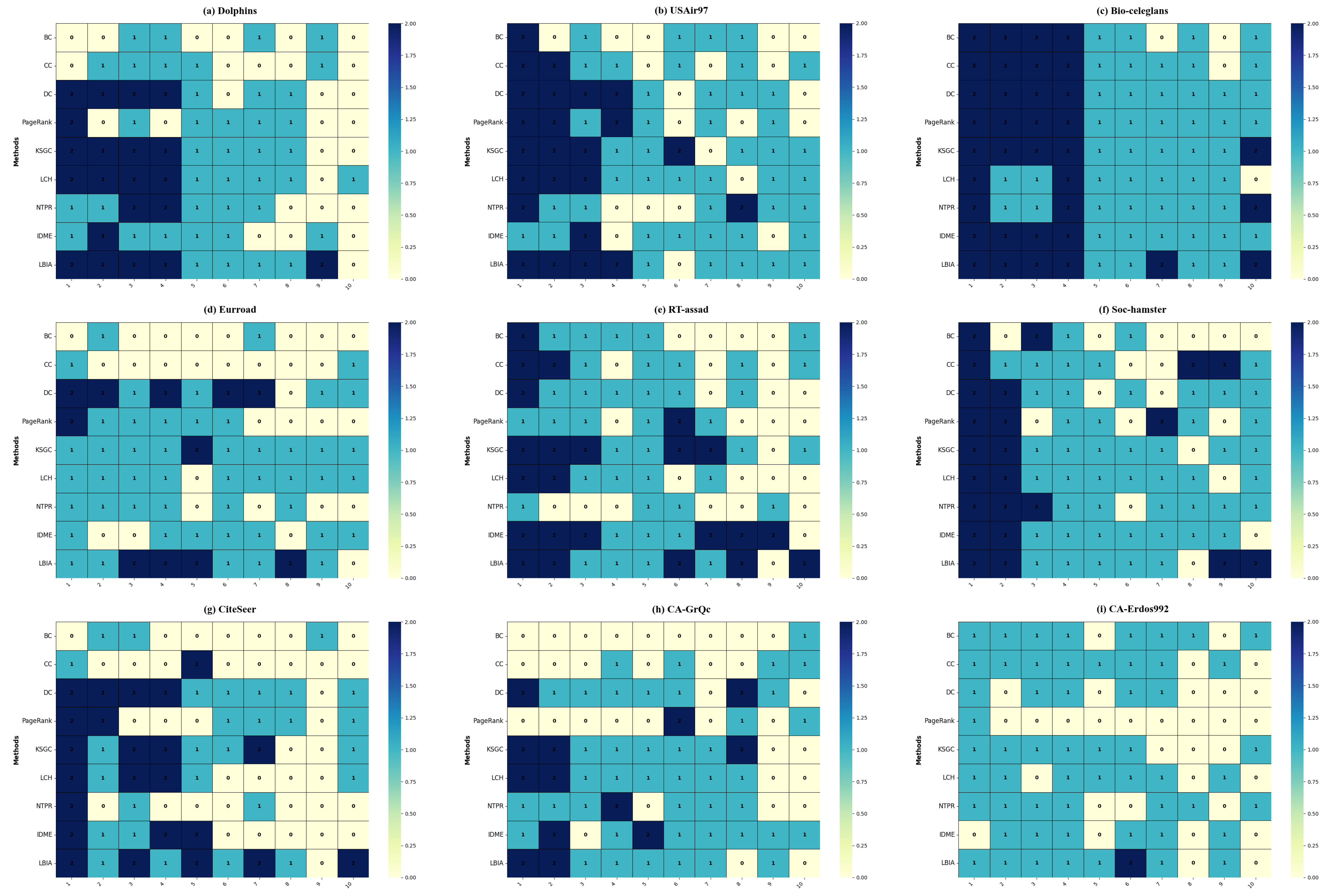
denotes the results of the top-10 nodes obtained by the different algorithms under the Dolphins network. Nodes that agree with the SIR ranking list are marked in red, nodes that differ are marked in blue, and nodes that do not appear in the SIR ranking list are not colored. Figure 5 summarizes the top-10 important nodes obtained from each comparison algorithm. Nodes that are consistent with the SIR ranking are colored dark blue, nodes with inconsistent rankings are colored blue, and nodes that do not appear in the SIR are colored yellow.

In the heatmap, each row represents the comparison between the important node ranking obtained by the algorithm and the SIR ranking. From the analysis, it can be observed that the LBIA algorithm achieved the highest number of nodes with consistent rankings with SIR on six networks: Dolphins, USAir97, Bio-celegans, Soc-hamser, CiteSeer, and CA-Erdos. It also had the largest number of identical nodes. Although the number of consistent nodes was not the highest on the Eurroad and RT-assad networks, it was second only to the algorithm with the highest count, and the number of identical nodes was the largest among the nine algorithms. On the CA-GrQc network, the LBIA algorithm also performed well for eight nodes and accurately identified the top-two nodes.

In summary, the LBIA algorithm was better at accurately identifying the top-10 key nodes in the network. Compared to the other algorithms, LBIA performed better in node ranking sequences.

5.4.2. Ranking Accuracy

To evaluate the performance of the LBIA algorithm more comprehensively, we used the Kendall metrics to assess the effectiveness of each algorithm. To make the results convincing, the infection probability $\beta$ in the SIR model started at 0.02 and increased by 0.01 each time. Different networks were propagated with different infection probabilities and the ranking results of each algorithm were compared. Figure 6 and the table demonstrate the Kendall values of each algorithm with different infection probabilities, which show that the LBIA algorithm achieved good results on the Dolphins, USAir97, Bio-celegans, Eurroad, RT-assad CA-GrQc, and CA-Erdos992 networks, and significantly outperformed the rest of the algorithms on the Soc-hamster and CiteSeer networks.

Table 3. The average Kendall $\tau$ value of nine algorithms under different propagation probabilities.

	BC	CC	DC	PageRank	KSGC	LCH	NTPR	IDME	LBIA
Dolphins	0.5970	0.5600	0.8483	0.7940	0.8597	0.0459	0.0467	0.8506	0.8633
USAir97	0.5264	0.7872	0.7470	0.5686	0.8412	0.1422	0.0759	0.8922	0.9067
Bio-celegans	0.4832	0.6230	0.6805	0.5486	0.8444	−0.0025	0.0005	0.8304	0.8459
Eurroad	0.4978	0.3234	0.6607	0.5154	0.7259	0.1630	0.1382	0.6401	0.7050
Rt-assad	−0.0024	0.0052	−0.0014	0.0093	0.0122	0.0089	0.0035	0.4280	0.4374
Soc-hamster	0.5530	0.7933	0.7529	0.2995	0.8333	0.2066	0.2603	0.8168	0.8355
CiteSeer	0.5470	0.4990	0.7170	0.3648	0.7790	0.0041	0.0261	0.6811	0.7458
CA-GrQc	0.1329	0.2679	0.1599	0.0326	0.2101	0.2269	0.1943	0.7311	0.7532
CA-Erdos992	0.0459	0.0948	0.0502	0.0209	0.0657	0.0794	0.0633	0.4674	0.5037

presents the average Kendall values of nine algorithms under different propagation probabilities.

5.4.3. Node Consistency

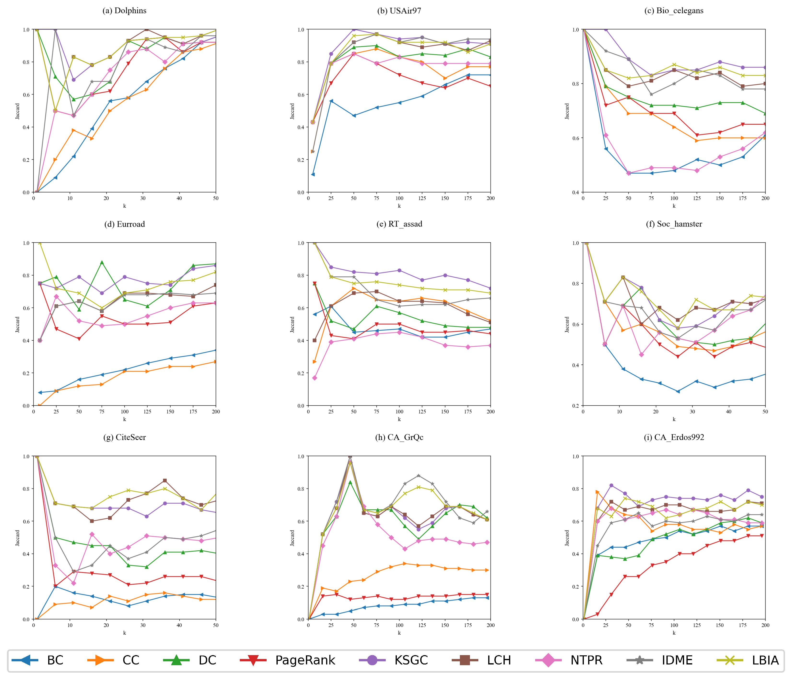
The Jaccard coefficient was used to measure the consistency of the ranking of the Top-k nodes, and the results are shown in Figure 7. The LBIA algorithm consistently achieved high Jaccard values across all nine networks, ranking first or second in each network. With the increase in the number of nodes, the Jaccard values of the LBIA algorithm were all above 0.6, and its recognition ability was stable and did not fluctuate significantly. The LBIA algorithm outperformed the other algorithms in terms of Jaccard similarity values across the four tightly interconnected networks and demonstrated a superior capability in identifying key nodes within general networks. These findings indicate that the LBIA algorithm is more effective at accurately identifying critical nodes in networks with dense interconnections.

5.4.4. Monotonicity Index

The accuracy and effectiveness of the algorithms are quite important, but also the differentiation ability of the algorithms in the network is also crucial. Currently, most algorithms use the monotonicity function Equation (12) to evaluate the differentiation ability of the algorithms.

Table 4. The ability of each algorithm to distinguish between different networks.

	BC	CC	DC	PageRank	KSGC	LCH	NTPR	IDME	LBIA
Dolphins	0.96	0.97	0.83	1.00	0.99	0.99	0.99	1.00	1.00
USAir97	0.70	0.99	0.86	1.00	0.99	0.99	1.00	1.00	1.00
Bio-celegans	0.87	0.99	0.79	1.00	1.00	0.99	1.00	1.00	1.00
Eurroad	0.94	1.00	0.44	1.00	0.91	0.94	0.99	1.00	1.00
RT-assad	0.21	0.98	0.21	0.98	0.97	0.98	1.00	0.98	1.00
Soc-hamster	0.71	0.98	0.90	0.95	0.99	0.98	0.99	0.99	1.00
CiteSeer	0.59	0.95	0.56	0.94	0.93	0.93	0.98	0.95	0.95
CA-GrQc	0.38	0.99	0.75	0.97	0.98	0.98	0.99	0.99	1.00
CA-Erdos992	0.17	0.99	0.23	0.99	0.99	0.99	1.00	0.99	1.00

shows the differentiation ability of the nine algorithms across the nine networks. The LBIA algorithm achieved a Mon value of 1 on eight networks, including four tightly interconnected networks. Although it did not reach 1 on the CiteSeer network, its differentiation ability was still 0.95, which was superior compared to the other algorithms. While CC, PageRank, KSGC, LCH, NTPR, and IDME also demonstrated strong differentiation abilities in the four tightly interconnected networks, none of them achieved a Mon value of 1. The differentiation ability of the BC algorithm and the DC algorithm fluctuated more, which indicates that these two algorithms depend on the specific network to differentiate the importance of nodes more accurately.

5.4.5. Correlation Index

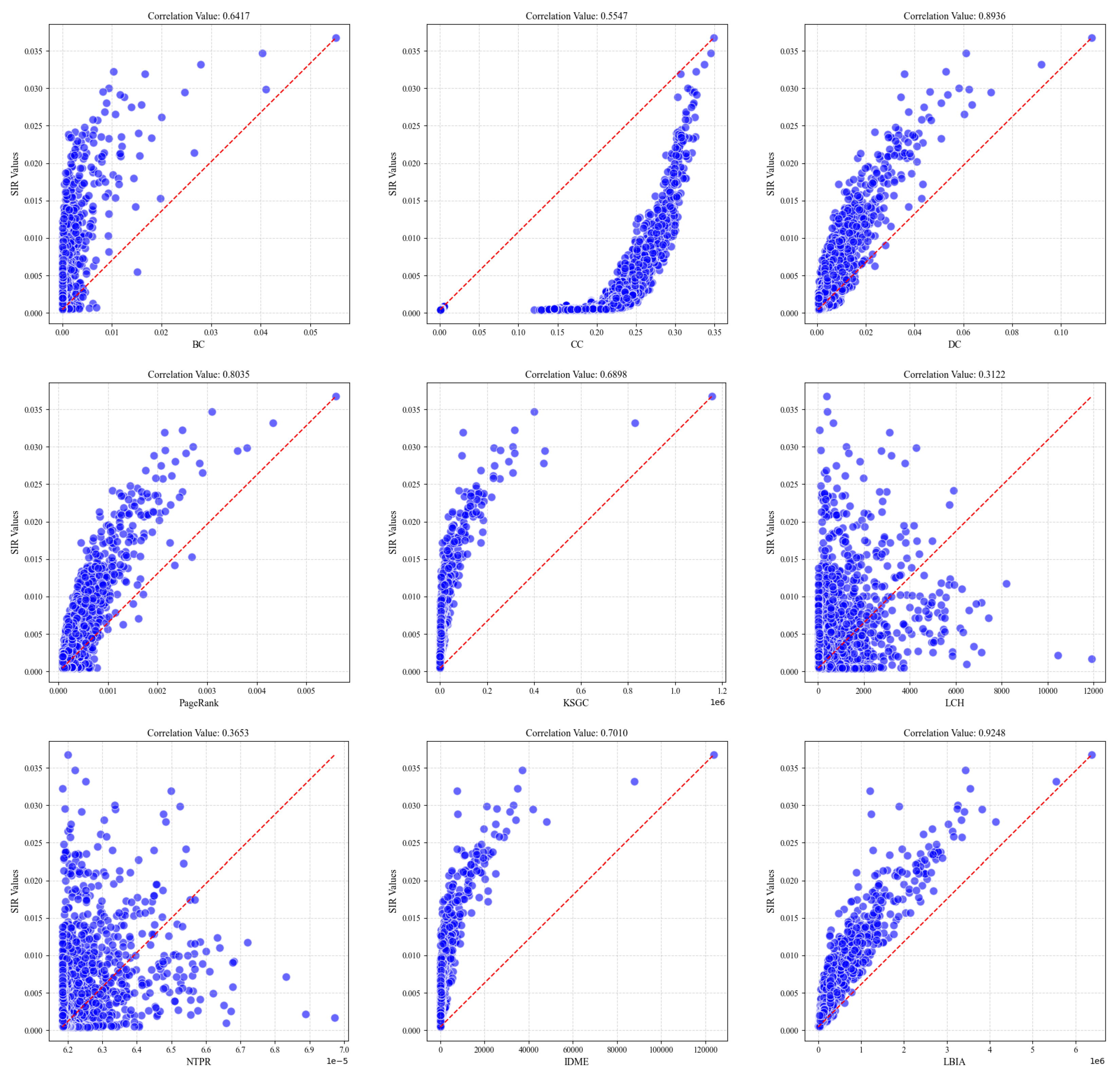
The role of the correlation coefficient is to measure the linear relationship between two variables. Specifically, by calculating the correlation between different algorithms and SIR, we can assess the consistency of different key node identification methods. A value of 1 indicates a perfect positive correlation, −1 indicates a perfect negative correlation, and 0 indicates no linear relationship. By plotting scatter plots, the effectiveness of the correlation between different algorithms can be visualized. Figure 8 shows the correlation coefficient values between different algorithms and SIR in the Soc-hamster network. In this highly interconnected network, the DC, KSGC, and IDME algorithms demonstrated relatively high correlation coefficients. The LBIA algorithm, which integrates node degree, node position, and the aggregation of propagated information, achieved a correlation coefficient of 0.9248. In contrast, the scatter plots of the remaining algorithms exhibit more dispersed distributions. This suggests that the LBIA algorithm exhibits a stronger correlation coefficient in tightly interconnected networks, highlighting its superior capability in identifying important nodes.

6. Conclusions

This paper proposes a critical node identification algorithm based on local balance and multi-layer neighbor information aggregation (LBIA). The local balance value is introduced to propagate and aggregate information, and the improved PKs algorithm is used to encapsulate the node’s individual information. These two types of information are then considered together to identify critical nodes in the network. This method addresses the issue of inaccurately identifying critical nodes in restricted regions. Furthermore, due to its low time complexity, it is suitable for large-scale networks.

We evaluated the performance of LBIA by comparing it with nine other algorithms across nine different networks. The experimental results show that LBIA achieved the best accuracy in identification, with an average Kendall value of 0.7330, while the average Kendall values of other algorithms ranged from 0.3 to 0.7. LBIA significantly outperformed the other algorithms on three of the networks, which all had a larger number of restricted regions. In terms of the accuracy of identifying the top-10 nodes, LBIA’s consistency ranged from 0.82 to 1. As the number of nodes increased, LBIA’s Jaccard values stabilized between 0.6 and 0.8 across different networks, while the other algorithms showed instability with network changes. In terms of distinguishing capability, LBIA achieved a monotonicity value of 1, with no nodes having identical values. LBIA exhibited the best overall performance across nine networks, particularly in tightly interconnected networks, where it outperformed the other algorithms in all three metrics. This indicates that the algorithm is broadly applicable to various network types and demonstrates distinct advantages in specific network configurations.

The LBIA algorithm improves on the limitations of the existing algorithms in terms of the bidirectional propagation of information and significantly reduces the problem of bias due to the repeated propagation of information during node identification by proposing the concept of the local balance value. Experimental results indicate that the algorithm exhibits superior performance across various network structures. Moreover, by only considering information from local neighborhood nodes, the LBIA algorithm not only ensures high accuracy in identification but also significantly reduces computational complexity. However, we did not consider the impact of the edge weight distribution on information propagation. As the research continues, we plan to extend LBIA to weighted and directed networks.

References

- Chen, L.; Xi, Y.; Dong, L.; Zhao, M.; Li, C.; Liu, X.; Cui, X. Identifying influential nodes in complex networks via Transformer. Inf. Process. Manag. 2024, 61, 103775. [Google Scholar] [CrossRef]
- Wang, L.; Mou, J.; Dai, B.; Tan, S.; Cai, M.; Chen, H.; Jin, Z.; Sun, G.; Lu, X. Influential nodes identification based on hierarchical structure. Chaos Solitons Fractals 2024, 186, 115227. [Google Scholar] [CrossRef]
- Gao, L.; Wang, W.; Shu, P.; Gao, H.; Braunstein, L.A. Promoting information spreading by using contact memory. Europhys. Lett. 2017, 118, 18001. [Google Scholar] [CrossRef]
- Zhang, X.; Zhu, J.; Wang, Q.; Zhao, H. Identifying influential nodes in complex networks with community structure. Knowl.-Based Syst. 2013, 42, 74–84. [Google Scholar] [CrossRef]
- Malliaros, F.D.; Rossi, M.E.G.; Vazirgiannis, M. Locating influential nodes in complex networks. Sci. Rep. 2016, 6, 19307. [Google Scholar] [CrossRef]
- Dang, F.; Zhao, X.; Yan, L.; Wu, K.; Li, S. Research on network intrusion response method based on Bayesian attack graph. In Proceedings of the 2023 3rd International Conference on Consumer Electronics and Computer Engineering (ICCECE), Guangzhou, China, 6–8 January 2023; pp. 639–645. [Google Scholar]
- Zhu, P.; Wang, X.; Li, S.; Guo, Y.; Wang, Z. Investigation of epidemic spreading process on multiplex networks by incorporating fatal properties. Appl. Math. Comput. 2019, 359, 512–524. [Google Scholar] [CrossRef]
- Zhou, M.Y.; Xiong, W.M.; Wu, X.Y.; Zhang, Y.X.; Liao, H. Overlapping influence inspires the selection of multiple spreaders in complex networks. Phys. A Stat. Mech. Its Appl. 2018, 508, 76–83. [Google Scholar] [CrossRef]
- Li, X.; Jusup, M.; Wang, Z.; Li, H.; Shi, L.; Podobnik, B.; Stanley, H.E.; Havlin, S.; Boccaletti, S. Punishment diminishes the benefits of network reciprocity in social dilemma experiments. Proc. Natl. Acad. Sci. USA 2018, 115, 30–35. [Google Scholar] [CrossRef]
- Wang, Z.; Bauch, C.T.; Bhattacharyya, S.; d’Onofrio, A.; Manfredi, P.; Perc, M.; Perra, N.; Salathé, M.; Zhao, D. Statistical physics of vaccination. Phys. Rep. 2016, 664, 1–113. [Google Scholar] [CrossRef]
- Chen, D.B.; Sun, H.L.; Tang, Q.; Tian, S.-Z.; Xie, M. Identifying influential spreaders in complex networks by propagation probability dynamics. Chaos Interdiscip. J. Nonlinear Sci. 2019, 29, 033113. [Google Scholar] [CrossRef]
- Ballinger, O. Insurgency as complex network: Image co-appearance and hierarchy in the PKK. Soc. Netw. 2023, 74, 182–205. [Google Scholar] [CrossRef]
- Wang, H.; Fang, Y.P.; Zio, E. Resilience-oriented optimal post-disruption reconfiguration for coupled traffic-power systems. Reliab. Eng. Syst. Saf. 2022, 222, 108408. [Google Scholar] [CrossRef]
- Li, Q.; Zhou, T.; Lü, L.; Chen, D. Identifying influential spreaders by weighted LeaderRank. Phys. A Stat. Mech. Its Appl. 2014, 404, 47–55. [Google Scholar] [CrossRef]
- Brin, S.; Page, L. The anatomy of a large-scale hypertextual web search engine. Comput. Netw. ISDN Syst. 1998, 30, 107–117. [Google Scholar] [CrossRef]
- Xu, G.; Meng, L. A novel algorithm for identifying influential nodes in complex networks based on local propagation probability model. Chaos Solitons Fractals 2023, 168, 113155. [Google Scholar] [CrossRef]
- Zhao, J.; Wang, Y.; Deng, Y. Identifying influential nodes in complex networks from global perspective. Chaos Solitons Fractals 2020, 133, 109637. [Google Scholar] [CrossRef]
- Bonacich, P. Factoring and weighting approaches to status scores and clique identification. J. Math. Sociol. 1972, 2, 113–120. [Google Scholar] [CrossRef]
- Freeman, L.C. Centrality in social networks: Conceptual clarification. In Social Network: Critical Concepts in Sociology; Routledge: Brighton, UK, 2002; Volume 1, pp. 238–263. [Google Scholar]
- Xu, G.Q.; Meng, L.; Tu, D.Q.; Yang, P.L. LCH: A local clustering H-index centrality measure for identifying and ranking influential nodes in complex networks. Chin. Phys. B 2021, 30, 088901. [Google Scholar] [CrossRef]
- Zareie, A.; Sheikhahmadi, A.; Jalili, M.; Fasaei, M.S.K. Finding influential nodes in social networks based on neighborhood correlation coefficient. Knowl.-Based Syst. 2020, 194, 105580. [Google Scholar] [CrossRef]
- Chen, D.; Lü, L.; Shang, M.S.; Zhang, Y.C.; Zhou, T. Identifying influential nodes in complex networks. Phys. A Stat. Mech. Its Appl. 2012, 391, 1777–1787. [Google Scholar] [CrossRef]
- Hajarathaiah, K.; Enduri, M.K.; Anamalamudi, S.; Reddy, T.S.; Tokala, S. Computing influential nodes using the nearest neighborhood trust value and pagerank in complex networks. Entropy 2022, 24, 704. [Google Scholar] [CrossRef] [PubMed]
- Shetty, R.D.; Bhattacharjee, S.; Dutta, A.; Namtirtha, A. GSI: An influential node detection approach in heterogeneous network using covid-19 as use case. IEEE Trans. Comput. Soc. Syst. 2022, 10, 2489–2503. [Google Scholar] [CrossRef]
- Yang, X.; Xiao, F. An improved gravity model to identify influential nodes in complex networks based on k-shell method. Knowl.-Based Syst. 2021, 227, 107198. [Google Scholar] [CrossRef]
- Zhou, M.Y.; Xu, R.Q.; Li, X.Y.; Liao, H. Identifying influential nodes to enlarge the coupling range of pinning controllability. J. Stat. Mech. Theory Exp. 2020, 9, 093401. [Google Scholar] [CrossRef]
- Sun, Z.; Sun, Y.; Chang, X.; Wang, F.; Wang, Q.; Ullah, A.; Shao, J. Finding critical nodes in a complex network from information diffusion and Matthew effect aggregation. Expert Syst. Appl. 2023, 233, 120927. [Google Scholar] [CrossRef]
- Watts, D.J.; Strogatz, S.H. Collective dynamics of ‘small-world’ networks. Nature 1998, 393, 440–442. [Google Scholar] [CrossRef]
- Hennig, C.; Hausdorf, B. Design of dissimilarity measures: A new dissimilarity between species distribution areas. In Data Science and Classification; Springer: Berlin/Heidelberg, Germany, 2006; pp. 29–37. [Google Scholar]
- Kitsak, M.; Gallos, L.K.; Havlin, S.; Liljeros, F.; Muchnik, L.; Stanley, H.E.; Makse, H.A. Identification of influential spreaders in complex networks. Nat. Phys. 2010, 6, 888–893. [Google Scholar] [CrossRef]
- Yang, Q.; Wang, Y.; Yu, S.; Wang, W. Identifying influential nodes through an improved k-shell iteration factor model. Expert Syst. Appl. 2024, 238, 122077. [Google Scholar] [CrossRef]
- Cohen, J.E. Infectious diseases of humans: Dynamics and control. JAMA 1992, 268, 3381. [Google Scholar] [CrossRef]
- Ellison, G. Implications of heterogeneous SIR models for analyses of COVID-19. Rev. Econ. Des. 2024, 28, 651–687. [Google Scholar] [CrossRef]
- Lalou, M.; Tahraoui, M.A.; Kheddouci, H. The critical node detection problem in networks: A survey. Comput. Sci. Rev. 2018, 28, 92–117. [Google Scholar] [CrossRef]
- Kendall, M.G. A new measure of rank correlation. Biometrika 1938, 30, 81–93. [Google Scholar] [CrossRef]
- Bae, J.; Kim, S. Identifying and ranking influential spreaders in complex networks by neighborhood corenes. Phys. A Stat. Mech. Its Appl. 2014, 395, 549–559. [Google Scholar] [CrossRef]
Figure 1.
The k-shell decomposition process: where the number represents the node ID. Nodes with the same color mean that they are in the same layer. Circles of different colors represent different layers.
Figure 2.
A simple network: due to the bidirectional propagation of information, nodes 2, 3, 4, and 5 have a value of 13 and node 1 has a value of 17, nodes 6, 7, 8, and 9 are edge nodes and have value of 1.
Figure 3.
A simple network: (a) Assign initial information to each node. (b) Information propagation between nodes. (c) Aggregate information from neighboring nodes. Where the number represents the node ID. Yellow node is source node and green nodes are first order neighbours of the source nodes. The arrow pointing is the direction of information propagation.
Figure 4.
Dolphins network visualization: where the number represents the node ID. Purple node is source node, green nodes are first order neighbours, orange nodes are second order neighbours.
Figure 5.
Top-10 nodes’ heatmaps for different algorithms on different networks and the legend: nodes that are consistent with the SIR ranking are colored dark blue, nodes with inconsistent rankings are colored blue, and nodes that do not appear in the SIR are colored yellow.
Figure 6.
Kendall values of different algorithms on different networks and the legend: The different colored lines represent the kendall values obtained by the different algorithms on the corresponding networks as the probability of propagation changes. The higher the kendall value, the more consistent the node ordering.
Figure 7.
The Jaccard value between the Top-k nodes for different algorithms: The different colored lines represent the Jaccard values obtained by the different algorithms on the corresponding networks as the probability of propagation changes. The higher the Jaccard value, the higher the number of nodes with the same ordering.
Figure 8.
Scatter Plot of correlation for different algorithms on the Soc-hamster network: the blue circles represent points with the algorithm value and the SIR value as coordinates. The red dash line represents the points that are on this line have a perfectly positive correlation property, and the further away from the line, the weaker the correlation.