Optimal Allocation of Water Resources in Irrigation Areas Considering Irrigation Return Flow and Uncertainty

Abstract

To improve the utilization rate of water resources in irrigation areas, this study established an uncertain water resource optimal allocation model considering the reuse of return flow, and it analyzed the impact of return flow reuse on irrigation efficiency, crop planting structure, and water resource allocation in irrigation areas. If only the optimal allocation of irrigation diversion is carried out, the net profit for the current years, short-term (2021–2040) planning years, and long-term (2041–2060) planning years will increase by USD [18.27, 24.18], [2.20, 2.47], and [3.02, 3.43] million, respectively, and the total planting area in the current years, short-term planning years, and long-term planning years will increase by 900 ha, 700 ha, and 1000 ha, respectively. Restricted by the total amount of irrigation water diversion, the irrigation water resources in the current years and the planning years are in deficit. When the channel return flow is optimized, the net profit of the current years and the short-term and long-term planning years will increase by USD [7.14, 7.97], [5.08, 5.63], and [4.4, 4.81] million, respectively. The total planting area in the current years and short-term and long-term planning years will increase by 2.6, 1.9, and 1.6 thousand ha, respectively, and the amount of irrigation water diversion will decrease by [12, 18], [18, 24], and [20, 26] million m³, respectively. Reasonable and optimized use of channel return flow can not only improve the irrigation efficiency of irrigation areas and avoid the impact of return flow discharge on the water quality of the Yellow River, but it can also reduce the cost of water extraction and save water resources.

1. Introduction

Water is essential for human survival, yet China faces a significant water shortage, with per capita freshwater resources being only a quarter of the global average [1,2]. In 2021, agriculture accounted for 61.5% of the country’s total water consumption, with the northwest region being the most water-deficient, possessing only 5.7% of the total water resources [3]. Despite this, over 80% of the water in the region is used for agriculture. Increasing industrial and domestic water consumption exacerbates the water supply–demand imbalance, hindering economic development in the northwest [4]. In the 1950s and 1970s, China constructed large irrigation systems in this region to meet water needs, particularly along the Yellow River in Gansu, Ningxia, and Shaanxi [5]. However, many of these systems suffer from poor infrastructure, leading to significant water wastage through return flow, which accounts for 40–60% of the diverted water [6]. This return flow also contributes to salinization, necessitating large-scale flushing to remove salt buildup. Managing irrigation water resources is crucial to alleviating water scarcity. Climate factors and agricultural practices further complicate the return flow, creating uncertainties that impact optimal water allocation. Enhancing return flow reuse can improve water efficiency and help address supply–demand imbalances in northwest China.

In recent years, researchers have concentrated on optimizing irrigation water management. Li et al. [7,8] developed a model for crop irrigation scheduling to address water scarcity, while Montazar et al. [9] created a nonlinear allocation model to maximize economic benefits, studying the combined use of surface water and groundwater in Iran. However, as water shortages and quality issues have worsened, the focus has shifted from economic maximization to multi-objective models that balance economic, water resource, and environmental sustainability [10]. Habibi et al. [11] employed particle swarm optimization and genetic algorithms to consider agricultural yields and prices in water allocation. Afzal et al. [12] optimized irrigation quotas and crop structure to maximize efficiency while managing groundwater quantity and quality. Guo et al. [13] focused on economic benefits and water resources, analyzing crop structure under varying water inflows. Yang et al. [14] applied queuing theory to optimize water allocation, addressing water diversion and crop demand. Cui et al. [15] combined fractional optimization and fuzzy constraints to balance water resources and economic profits. Karamouz et al. [16] developed a model incorporating surface sewage to minimize agricultural intake costs and manage groundwater levels. Bazargan-Lari et al. [17] analyzed the relationship between groundwater levels, quality, and costs to optimize allocation. As research progresses, it is hoped that water scarcity will be somewhat alleviated. However, uncertainty in water resource systems due to human and natural factors complicates management and decision-making.

The water resource system encompasses processes such as water transfer, transmission, distribution, and utilization, with uncertainties primarily arising in water supply, demand, and the interplay between the two [18]. Uncertainties in water supply stem from factors like evaporation, leakage, and the limited exploitation of sources such as rivers, lakes, and groundwater. Demand uncertainties are influenced by fluctuating agricultural water needs, which are affected by climate and crop conditions. The relationship between supply and demand further contributes to uncertainty; excess supply results in waste, while insufficient supply leads to crop shortages. Water allocation efficiency is generally measured using economic indicators, which can be influenced by market factors, introducing additional uncertainty [19]. To address these uncertainties, both domestic and international scholars have investigated optimization models. Maqsood et al. [20] utilized interval numbers to model uncertain water resources, providing crop water allocation schemes under varying inflows. Fu et al. [21] focused on minimizing water costs while considering risk factors to enhance system stability. Huang et al. [22] integrated two-stage stochastic planning with imprecise quadratic programming to optimize water allocation and improve efficiency. Yang et al. [23] developed a nonlinear fuzzy interval model for water resource optimization, demonstrating its effectiveness in enhancing economic benefits. Li et al. [24] proposed an uncertainty planning model to address irrigation shortages and boost crop productivity. Wang et al. [25] employed statistical models and neural networks to optimize irrigation under different climate scenarios. Yue et al. [26] created a fuzzy interval model to tackle water management issues and maximize system benefits. Guo et al. [27] showcased a multi-objective optimization model to improve water supply efficiency, while Gong et al. [28] developed a model incorporating crop price uncertainty to optimize water allocation.

In summary, research on the optimal allocation of water resources in irrigation areas has evolved from focusing on single objectives to multiple objectives, single sources to multiple sources, single levels to multiple levels, static to dynamic models, and certainty to uncertainty. Currently, most studies on optimal water resource allocation concentrate on river inflow and groundwater, with limited research considering the reuse of return flow in irrigation areas, especially under the uncertainty of return flow. This paper takes the Jingdian Irrigation District in Northwest China as a case study and establishes an optimal allocation model of water resources that accounts for both the reuse and uncertainty of return flow. It analyzes the impact of return flow reuse on irrigation efficiency, crop planting structure, and water resource allocation within the district. The study aims to provide theoretical support for the efficient utilization of water resources in irrigation districts.

2. Materials and Methods

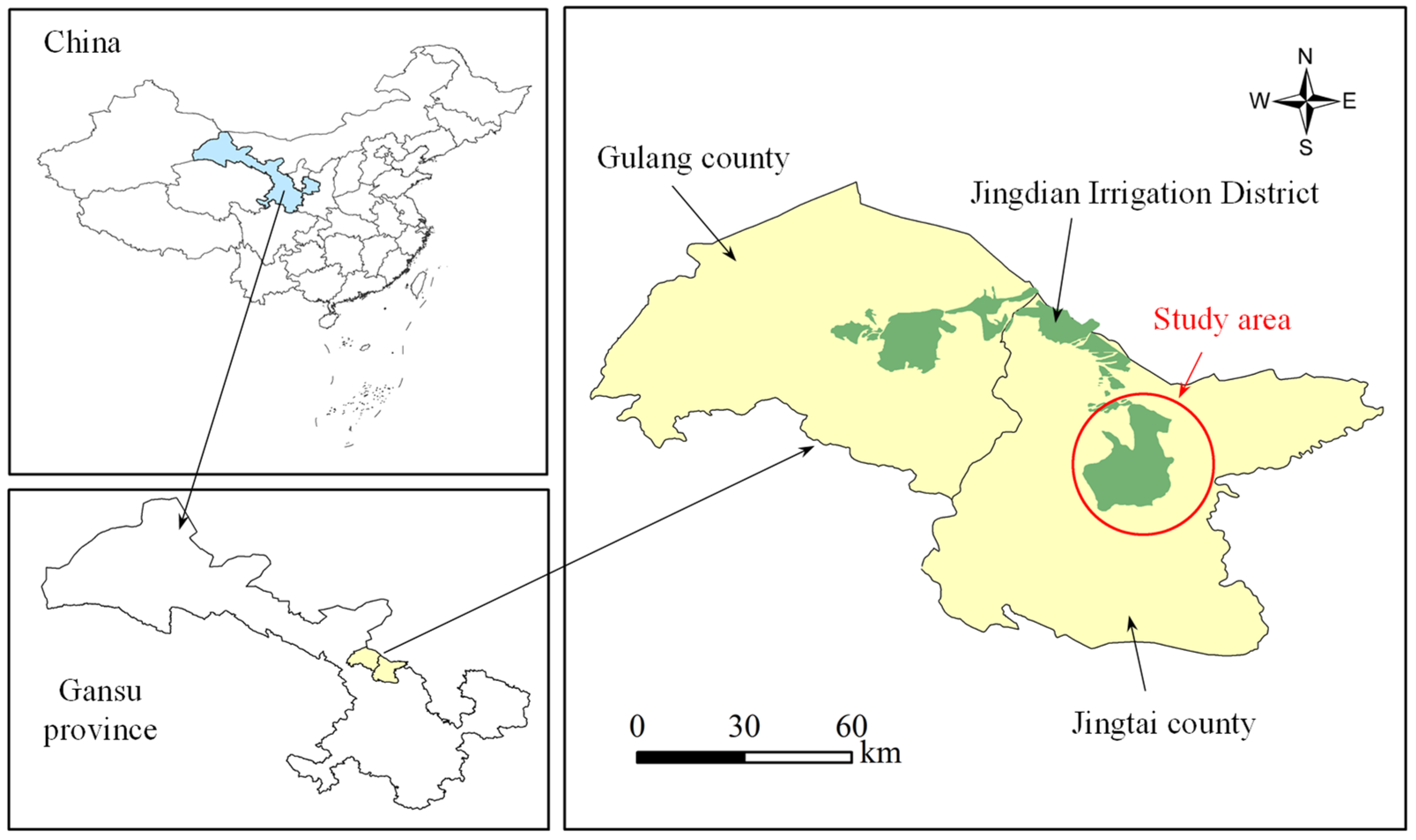
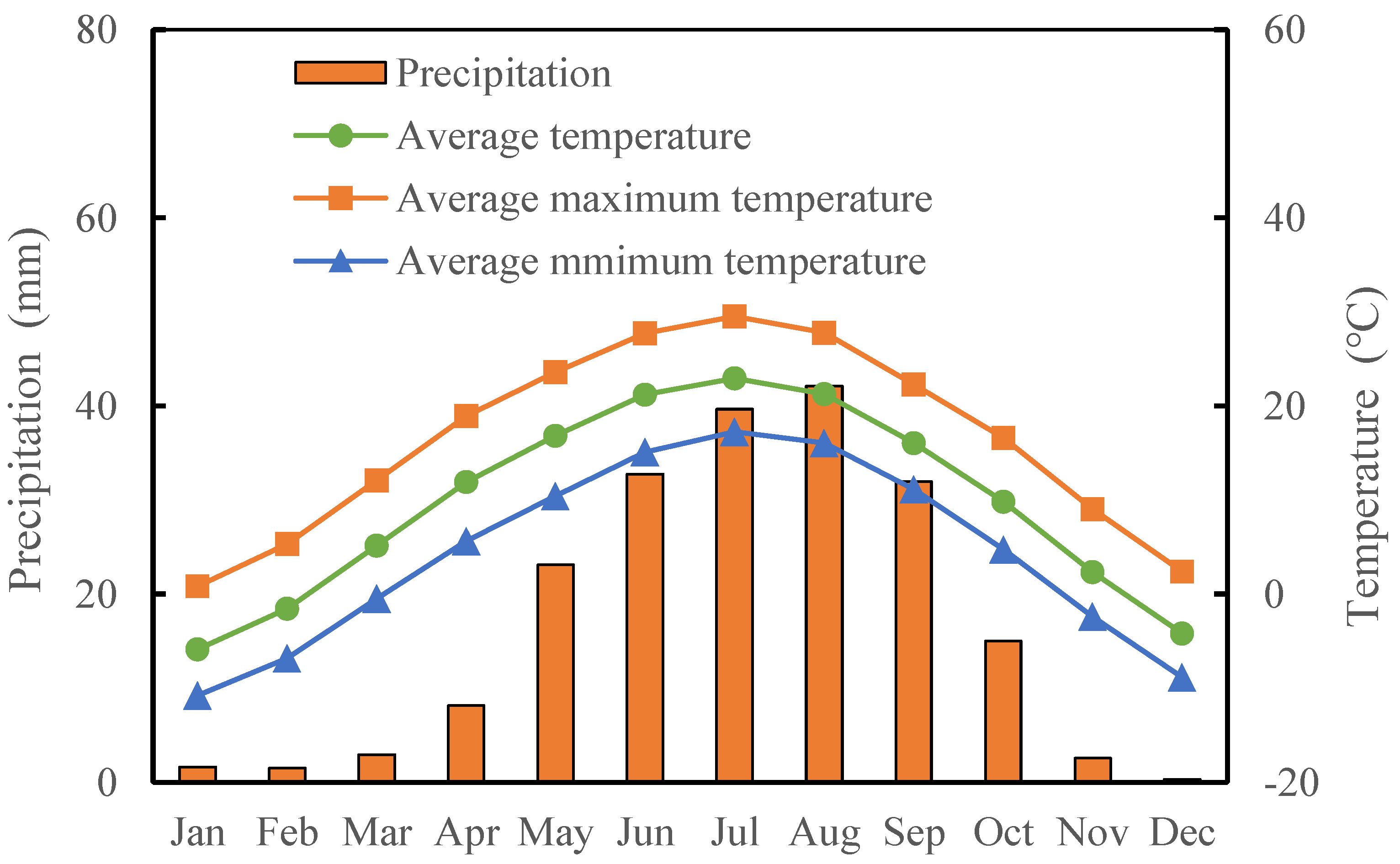
2.1. Study Area

The Jingdian Electric Power Irrigation Project in Gansu Province is a significant irrigation initiative located in northwest China. It is characterized by high lift, large flow, and numerous stages. The project supports agricultural irrigation in Jingtai County, Gulang County, and Minqin County in Gansu Province, as well as parts of Alashan Left Banner in Inner Mongolia. The Jingdian Irrigation District spans Jingtai County and Gulang County in central Gansu Province (see Figure 1), bordered by the Tengger Desert to the north, Changling Mountain to the south, and the Yellow River to the east. This large-scale irrigation area was established by the state to address issues of drought, water scarcity, and land desertification, along with the southward movement of deserts in Jingtai County and Gulang County. The study area, located in the eastern part of the Jingdian Irrigation District, covers 351.3 km², with an irrigated area of 235.4 km². The surface elevation ranges from 1300 to 1710 m above sea level, featuring a terrain that is higher in the west and lower in the east. The region consists of numerous mountains and hills, forming several basins, including the Caowotan Basin, Si’ertan Basin, Luyang Basin, and Xingquan Basin. The flat terrain in these basins is conducive to farming and irrigation. The primary food crops in the irrigation area are potatoes, spring wheat, and corn, while the main cash crops include forest fruits, goji berries, flax, and melons.

The study area belongs to the temperate continental arid climate, characterized by drought and little rain, large temperature differences between day and night, sufficient sunshine, high evaporation intensity, and windy sand. According to the observation data of Jingtai County Meteorological Observation Station from 1960 to 2020, the precipitation in the irrigation area is relatively small, with annual precipitation of 104~298 mm, annual average precipitation of 191 mm, and an annual average temperature of 8.8 °C. It can be seen in Figure 2 that the average monthly precipitation in the study area is extremely uneven, mainly concentrated in June to September, accounting for 73% of the annual precipitation. The monthly average temperature shows a single peak distribution, with the highest in July and the lowest in January. According to the monitoring results of the evaporating dish, the average annual evaporation of the water surface is 2290 mm, the maximum annual evaporation of the water surface is 2752 mm, the ratio of evaporation to precipitation is 1:18, and the drought index is up to 3.0, belonging to the extremely arid area. The average number of sunshine hours for many years in the irrigation area is 2726 h, and the average wind speed is 1.8 m/s. The frequency of dust storms in the region is relatively high, mostly in late spring and early summer.

2.2. Optimal Allocation of Water Resources

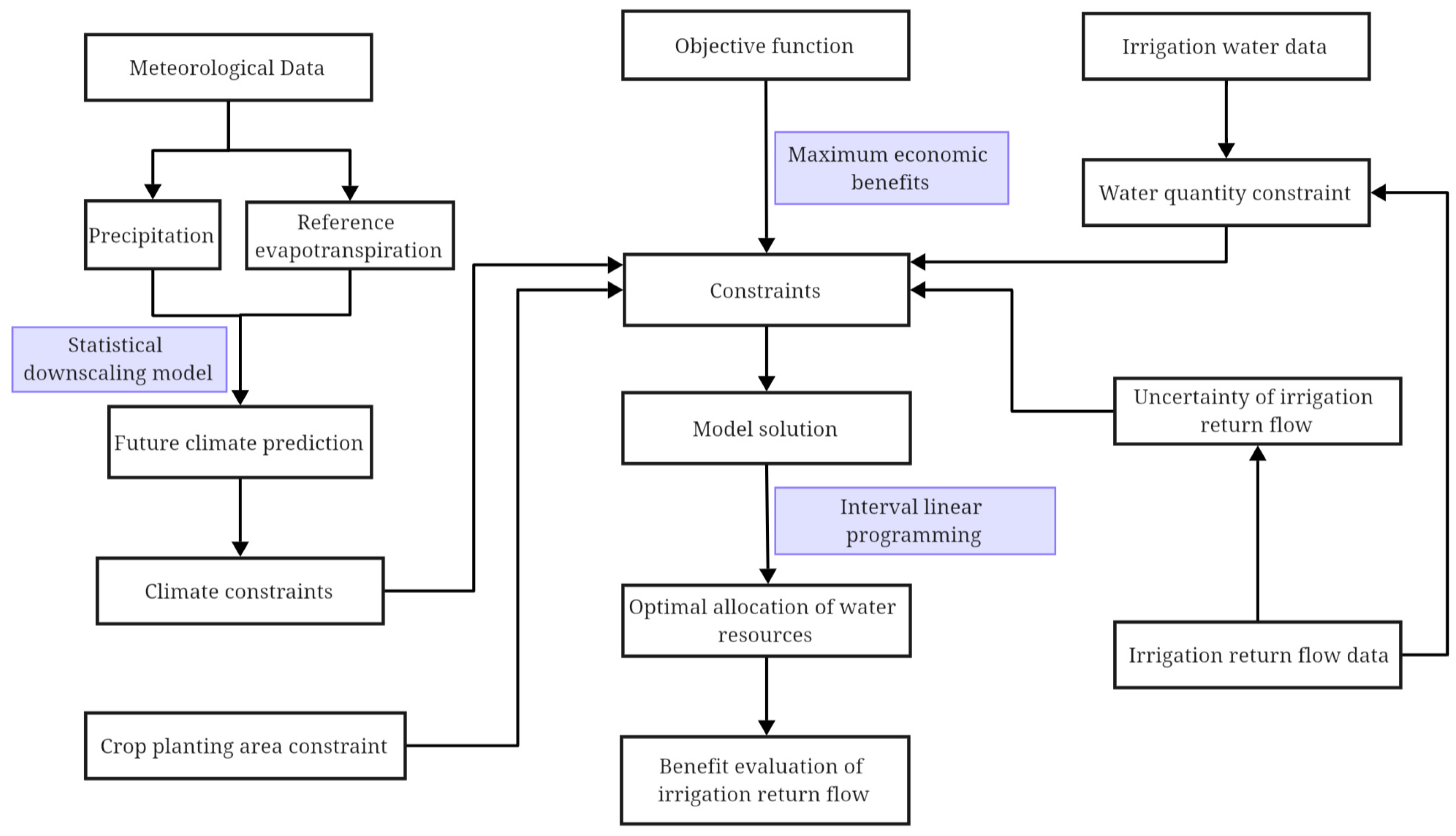
2.2.1. Process of Optimal Allocation

To achieve the efficient reuse of irrigation return flow, this study developed a water resource optimization allocation model that accounts for irrigation return water and associated uncertainties. The process is illustrated in Figure 3. The first step involves establishing an objective function aimed at maximizing economic benefits. The second step defines constraints related to climate, crop planting area, irrigation water volume, and irrigation return flow. In the third step, interval linear programming is employed to solve the optimization model. Finally, the fourth step optimizes the allocation of water resources and evaluates the benefits of irrigation return flow.

2.2.2. Statistical Downscaling Model

Regional climate change significantly impacts the water cycle processes in irrigation areas, making the study of future climate change crucial for agricultural production. General circulation models (GCMs) are essential tools for predicting future climate change. However, the low resolution of these models limits their effectiveness in studying regional climate change. Downscaling technology addresses this issue effectively and is widely used in forecasting regional meteorological factors. The Statistical Downscaling Model (SDSM) utilizes multiple regression principles and a weather generator to establish an empirical statistical relationship between large-scale predictors and regional (or station) prediction variables, thereby enabling climate prediction. Precipitation and reference evapotranspiration are critical factors in determining irrigation water demand and influencing irrigation water diversion and return flow [29,30]. Previous studies have demonstrated that changes in precipitation, and reference evapotranspiration can be accurately predicted using the SDSM model. This study, therefore, focuses on predicting and analyzing these two meteorological factors based on the SDSM model. The SDSM model divides the prediction of daily precipitation and reference evapotranspiration into three steps. First, reference evapotranspiration is calculated using the Penman–Monteith formula based on observed meteorological data. Second, the statistical relationship between prediction variables and predictors is established, and the model parameters are determined. Third, estimated data from GCMs (HadCM3 under the B2 scenario) are used as input for the SDSM model to simulate changes in precipitation and reference evapotranspiration.

2.2.3. Interval Linear Programming

Due to climate change and human activities, numerous uncertainties exist in the supply and demand system of agricultural water resources. Traditional deterministic programming models, which neglect the impact of such uncertainties, diminish the referential value of research outcomes. To address these uncertainties, parameters or variables can be represented by interval numbers in a linear programming model [31]. This approach not only yields relatively stable solutions without requiring specific distribution information of the parameters and variables but also manages the uncertainties within the objective function and the constraints of the model [32,33]. The general form of an interval linear programming model is as follows [28]:

(1)

Objective function:

$$\mathrm{Max}{\mathrm{f}}^{\pm }={\mathrm{c}}^{\pm }·{\mathrm{x}}^{\pm },$$

(1)

(2)

Constraints:

$${\mathrm{a}}^{\pm }·{\mathrm{x}}^{\pm }\le {\mathrm{b}}^{\pm },$$

(2)

$${\mathrm{x}}^{\pm }\ge 0,$$

(3)

where ${\mathrm{a}}^{\pm },{\mathrm{b}}^{\pm },{\mathrm{c}}^{\pm },{\mathrm{x}}^{\pm }$ all represent the interval number; “−” represents the lower limit of the interval; and “+” represents the upper limit of the interval.

In order to solve the above model, it can be transformed into two linear programming submodels [34]:

(1)

Upper linear programming model

• Objective function:

  $$\mathrm{Max}{\mathrm{f}}^{+}=\sum _{\mathrm{j}=1}^{\mathrm{k}} {\mathrm{c}}_{\mathrm{j}}^{+}·{\mathrm{x}}_{\mathrm{j}}^{+}+\sum _{\mathrm{j}=\mathrm{k}+1}^{\mathrm{n}} {\mathrm{c}}_{\mathrm{j}}^{+}·{\mathrm{x}}_{\mathrm{j}}^{-},$$

  (4)
• Constraints:

  $$\sum _{\mathrm{j}=1}^{\mathrm{k}} {\left|{\mathrm{a}}_{\mathrm{i}\mathrm{j}}\right|}^{-}\mathrm{Sign}\left({\mathrm{a}}_{\mathrm{i}\mathrm{j}}^{-}\right){\mathrm{x}}_{\mathrm{j}}^{+}+\sum _{\mathrm{j}=\mathrm{k}+1}^{\mathrm{n}} {\left|{\mathrm{a}}_{\mathrm{i}\mathrm{j}}\right|}^{+}\mathrm{Sign}\left({\mathrm{a}}_{\mathrm{i}\mathrm{j}}^{+}\right){\mathrm{X}}_{\mathrm{j}}^{-}\le {\mathrm{b}}_{\mathrm{i}}^{+},$$

  (5)

  $${\mathrm{x}}_{\mathrm{j}}^{+}\ge 0,{\mathrm{x}}_{\mathrm{j}}^{-}\ge 0,\forall \mathrm{j},$$

  (6)

(2)

Lower-level linear programming model

• Objective function:

  $$\mathrm{Max}{\mathrm{f}}^{-}=\sum _{\mathrm{j}=1}^{\mathrm{k}} {\mathrm{c}}_{\mathrm{j}}^{-}·{\mathrm{x}}_{\mathrm{j}}^{-}+\sum _{\mathrm{j}=\mathrm{k}+1}^{\mathrm{n}} {\mathrm{c}}_{\mathrm{j}}^{-}·{\mathrm{x}}_{\mathrm{j}}^{+},$$

  (7)
• Constraints:

  $$\sum _{\mathrm{j}=1}^{\mathrm{k}} {\left|{\mathrm{a}}_{\mathrm{i}\mathrm{j}}\right|}^{+}\mathrm{Sign}\left({\mathrm{a}}_{\mathrm{i}\mathrm{j}}^{+}\right){\mathrm{x}}_{\mathrm{j}}^{-}+\sum _{\mathrm{j}=\mathrm{k}+1}^{\mathrm{n}} {\left|{\mathrm{a}}_{\mathrm{i}\mathrm{j}}\right|}^{-}\mathrm{Sign}\left({\mathrm{a}}_{\mathrm{i}\mathrm{j}}^{-}\right){\mathrm{x}}_{\mathrm{j}}^{+}\le {\mathrm{b}}_{\mathrm{i}}^{-},$$

  (8)

  $${\mathrm{x}}_{\mathrm{j}}^{-}\le {\mathrm{x}}_{\mathrm{jopt} }^{+},\mathrm{j}=\mathrm{1,2},\dots ,\mathrm{k},$$

  (9)

  $${\mathrm{x}}_{\mathrm{j}}^{+}\ge {\mathrm{x}}_{\mathrm{j}\mathrm{o}\mathrm{p}\mathrm{t}}^{-},\mathrm{j}=\mathrm{k}+1,\mathrm{k}+2,\dots ,\mathrm{n},$$

  (10)

  $${\mathrm{x}}_{\mathrm{j}}^{+}\ge 0,{\mathrm{x}}_{\mathrm{j}}^{-}\ge 0,\forall \mathrm{j},$$

  (11)

  where Sign() represents the sign function; ${\mathrm{x}}^{+}$ and ${\mathrm{x}}^{-}$ represent interval variables with positive and negative coefficients in the objective function, respectively.

The lower linear programming model is solved to obtain ${\mathrm{f}}_{\mathrm{o}\mathrm{p}\mathrm{t}}^{-}$, ${\mathrm{x}}_{\mathrm{jopt} }^{-}\left(\mathrm{j}=\mathrm{1,2},\cdots ,{\mathrm{k}}_1\right)$ and ${\mathrm{X}}_{\mathrm{jopt} }^{+}\left(\mathrm{j}={\mathrm{k}}_1+1,{\mathrm{k}}_1+2,\cdots ,\mathrm{n}\right)$.

The interval optimization results obtained by solving the above two sub-models can be expressed as ${\mathrm{x}}_{\mathrm{jopt} }^{\pm }=\left[{\mathrm{x}}_{\mathrm{jopt} }^{-},{\mathrm{x}}_{\mathrm{jopt} }^{+}\right]$ and ${\mathrm{f}}_{\mathrm{jopt} }^{\pm }=\left[{\mathrm{f}}_{\mathrm{jopt} }^{-},{\mathrm{f}}_{\mathrm{jopt} }^{+}\right]$.

2.2.4. Establishment of Optimal Allocation Model of Water Resources

The Jingdian Irrigation District is dry and lacks water. The Yellow River Committee and Gansu Province approved the study area to lift 148 million m³ of water from the Yellow River every year. Under the condition of limited irrigation and diversion, the existing irrigation water resources and cultivated land resources should be reasonably optimized. The Yellow River diversion and return flow are important irrigation water resources in irrigation areas. To maximize net profit, an optimal allocation model for uncertain water resources was established. This model operates under two modes: one that only considers irrigation diversion (model I) and another that simultaneously considers irrigation diversion and return flow (model II).

(1)

Objective function:

$$\mathrm{Max}{\mathrm{F}}^{\pm }=\sum _{\mathrm{i}=1}^7 \left({\mathrm{P}}_{\mathrm{i}}^{\pm }·{\mathrm{A}}_{\mathrm{i}}·{\mathrm{Y}}_{\mathrm{i}}\right)-\sum _{\mathrm{i}=1}^7 {\mathrm{Q}}_{\mathrm{i}}·{\mathrm{A}}_{\mathrm{i}}^{\pm }·\mathrm{C}-\sum _{\mathrm{i}=1}^7 {\mathrm{A}}_{\mathrm{i}}·{\mathrm{T}}_{\mathrm{i}},$$

(12)

where i represents the crop code (1: spring wheat, 2: corn, 3: flax, 4: potato, 5: melon, 6: goji berry, 7: forest fruits); ${\mathrm{F}}^{\pm }$ represents net profit (interval number), USD; ${\mathrm{P}}_{\mathrm{i}}^{\pm }$ represents the unit price of the i-th crop, USD/kg; ${\mathrm{A}}_{\mathrm{i}}$ represents the planting area of the i-th crop , ha; ${\mathrm{Y}}_{\mathrm{i}}$ is the yield per unit area of the i-th crop, kg/ha; ${\mathrm{Q}}_{\mathrm{i}}$ is the net irrigation quota of the i-th crop, m³/ha; C is the unit price of irrigation water, USD/m³; ${\mathrm{T}}_{\mathrm{i}}$ represents the planting cost of the i-th crop, including the cost of pesticides, fertilizers, seeds, etc., in USD/ha.

(2)

Constraints:

a.

Irrigation water constraint

When only the optimal allocation of irrigation water diversion is considered (model I), the gross irrigation water volume should not be greater than the irrigation water diversion volume. If the optimal allocation of irrigation diversion and return flow is also considered (model II), the gross irrigation water volume should not be greater than the sum of irrigation diversion and return flow. Therefore, the net irrigation quota shall meet the following constraints:

$$\left\{\begin{array}{cc}\sum _{\mathrm{i}=1}^7 {\displaystyle \frac{{\mathrm{Q}}_{\mathrm{i}}}{{\eta }_{\mathrm{u}}}}·{\mathrm{A}}_{\mathrm{i}}\le {\mathrm{Q}}_{\mathrm{d}}& \left(\mathrm{M}\mathrm{o}\mathrm{d}\mathrm{e}\mathrm{l} \mathrm{I}\right)\\ \sum _{\mathrm{i}=1}^7 {\displaystyle \frac{{\mathrm{Q}}_{\mathrm{i}}}{{\eta }_{\mathrm{u}}}}·{\mathrm{A}}_{\mathrm{i}}\le {\mathrm{R}\mathrm{F}}^{\pm }+{\mathrm{Q}}_{\mathrm{d}}& \left(\mathrm{M}\mathrm{o}\mathrm{d}\mathrm{e}\mathrm{l} \mathrm{I}\mathrm{I}\right)\end{array}\right.,$$

(13)

where ${\mathrm{Q}}_{\mathrm{d}}$ represents the maximum irrigation diversion, m³; ${\eta }_{\mathrm{u}}$ is the irrigation water utilization coefficient; and ${\mathrm{R}\mathrm{F}}^{\pm }$ refers to the annual return flow, m³.

The relationship between return flow and irrigation diversion in model II can be expressed as follows:

$${\mathrm{R}\mathrm{F}}^{\pm }={\mathrm{b}}^{\pm }·{\mathrm{Q}}_{\mathrm{i}},$$

(14)

where ${\mathrm{b}}^{\pm }$ represents the regression coefficient, m³.

•    b.

  Water balance constraint

The total water demand of crops consists of net irrigation quota and effective precipitation. Therefore, the crop water demand should meet:

$$10\sum _{\mathrm{i}=1}^7 \sum _{\mathrm{j}=1}^{12} {\mathrm{E}\mathrm{T}}_{\mathrm{i}\mathrm{j}}=10\sum _{\mathrm{i}=1}^7 \sum _{\mathrm{j}=1}^{12} {\mathrm{P}\mathrm{E}}_{\mathrm{i}\mathrm{j}}+\sum _{\mathrm{i}=1}^7{\mathrm{Q}}_{\mathrm{i}},$$

(15)

$${\mathrm{E}\mathrm{T}}_{\mathrm{i}\mathrm{j}}={\mathrm{K}\mathrm{c}}_{\mathrm{i}\mathrm{j}}·{\mathrm{E}\mathrm{T}}_{0 \mathrm{i}\mathrm{j}},$$

(16)

where j represents the month; ${\mathrm{P}\mathrm{E}}_{\mathrm{i}\mathrm{j}}$ is the effective precipitation of the i-th crop in the j-th month, mm; ${\mathrm{E}\mathrm{T}}_{\mathrm{i}\mathrm{j}}$ is the crop water demand of the i-th crop in the j-th month, mm; ${\mathrm{K}\mathrm{c}}_{\mathrm{i}\mathrm{j}}$ is the crop coefficient of the i-th crop in the j-th month, mm; and ${\mathrm{E}\mathrm{T}}_{0 \mathrm{i}\mathrm{j}}$ represents the reference evapotranspiration of the i-th crop in the j-th month, mm.

•    c.

  Crop area constraint

The multiple cropping index of crops in the study area is 1, and the total planting area of each crop should not be greater than the total planting area. In addition, affected by farmers’ farming practices, the planting area of various crops should be within a reasonable range, and the interval value formed by the current planting structure from 2001 to 2020 should be used as the planting area range of different crops. Therefore, the crop planting area should meet the following requirements:

$$\sum _{\mathrm{i}=1}^7 {\mathrm{A}}_{\mathrm{i}}\le {\mathrm{A}}_{\mathrm{t}\mathrm{o}\mathrm{t}},$$

(17)

$${\mathrm{A}}_{\mathrm{i}\mathrm{m}\mathrm{i}\mathrm{n}}\le {\mathrm{A}}_{\mathrm{i}}\le {\mathrm{A}}_{\mathrm{i}\mathrm{m}\mathrm{a}\mathrm{x}},$$

(18)

where ${\mathrm{A}}_{\mathrm{t}\mathrm{o}\mathrm{t}}$ represents the total cultivated area, ha; ${\mathrm{A}}_{\mathrm{i}\mathrm{m}\mathrm{a}\mathrm{x}}$ represents the maximum planting area of the i-th crop, ha; and ${\mathrm{A}}_{\mathrm{i}\mathrm{m}\mathrm{i}\mathrm{n}}$ represents the minimum planting area of the i-th crop, ha.

•    d.

  Non-negative constraint

Crop planting area shall meet non-negative constraints:

$${\mathrm{A}}_{\mathrm{i}}\ge 0,$$

(19)

2.2.5. Model Parameter

(1)

Effective precipitation

Effective precipitation is the key factor affecting the optimal allocation of water resources. The effective precipitation in the current years (2001~2020) is calculated according to the previous calculation results, and the effective precipitation in the short-term years (2021~2040) and long-term years (2041~2060) is calculated according to the precipitation utilization rate in the current years.

Table 1. Monthly precipitation (mm) during the crop period.

Period.	Mar.	Apr.	May	Jun.	Jul.	Aug.	Sep.	Oct.
Current	3.0	8.1	23.3	32.0	40.6	43.2	31.3	14.8
Short-term	2.9	10.2	22.4	35.4	46.7	49.0	30.0	16.5
Long-term	2.0	10.8	22.8	37.5	49.5	52.0	28.8	17.5

shows the annual distribution of annual average precipitation in different periods,

Table 2. Precipitation utilization rate of different crops.

Crop type	Mar.	Apr.	May	Jun.	Jul.	Aug.	Sep.	Oct.
Spring wheat	0.46	0.33	0.51	0.42	0.21	0.00	0.00	0.00
Corn	0.00	0.49	0.51	0.49	0.72	0.66	0.50	0.32
Flax	0.47	0.32	0.51	0.51	0.55	0.27	0.00	0.00
Potato	0.00	0.03	0.65	0.50	0.72	0.66	0.48	0.00
Melon	0.47	0.32	0.51	0.44	0.29	0.00	0.00	0.00
Goji berry	0.00	0.02	0.62	0.48	0.69	0.57	0.35	0.00
Forest fruits	0.47	0.32	0.51	0.48	0.72	0.66	0.41	0.14

shows the precipitation utilization rate of different crops, and

Table 3. Monthly effective precipitation (mm) during the crop period.

Period	Crop Period	Mar.	Apr.	May	Jun.	Jul.	Aug.	Sep.	Oct.
Current	Spring wheat	1.4	2.7	11.9	13.4	8.5	0.0	0.0	0.0
	Corn	0.0	4.0	11.9	15.7	29.2	28.5	15.7	4.7
	Flax	1.4	2.6	11.9	16.3	22.3	11.7	0.0	0.0
	Potato	0.0	0.2	15.1	16.0	29.2	28.5	15.0	0.0
	Melon	1.4	2.6	11.9	14.1	11.8	0.0	0.0	0.0
	Goji berry	0.0	0.2	14.4	15.4	28.0	24.6	11.0	0.0
	Forest fruits	1.4	2.6	11.9	15.4	29.2	28.5	12.8	2.1
Short-term	Spring wheat	1.3	3.4	11.4	14.9	9.8	0.0	0.0	0.0
	Corn	0.0	5.0	11.4	17.3	33.6	32.3	15.0	5.3
	Flax	1.4	3.3	11.4	18.1	25.7	13.2	0.0	0.0
	Potato	0.0	0.3	14.6	17.7	33.6	32.3	14.4	0.0
	Melon	1.4	3.3	11.4	15.6	13.5	0.0	0.0	0.0
	Goji berry	0.0	0.2	13.9	17.0	32.2	27.9	10.5	0.0
	Forest fruits	1.4	3.3	11.4	17.0	33.6	32.3	12.3	2.3
Long-term	Spring wheat	0.9	3.6	11.6	15.8	10.4	0.0	0.0	0.0
	Corn	0.0	5.3	11.6	18.4	35.6	34.3	14.4	5.6
	Flax	0.9	3.5	11.6	19.1	27.2	14.0	0.0	0.0
	Potato	0.0	0.3	14.8	18.8	35.6	34.3	13.8	0.0
	Melon	0.9	3.5	11.6	16.5	14.4	0.0	0.0	0.0
	Goji berry	0.0	0.2	14.1	18.0	34.2	29.6	10.1	0.0
	Forest fruits	0.9	3.5	11.6	18.0	35.6	34.3	11.8	2.5

shows the effective precipitation of different crops in different periods.

(2)

Reference evapotranspiration and crop water demand

According to the Penman–Monteith formula and crop coefficient method, reference evapotranspiration and crop water demand in different periods are calculated. The calculation results can be found in

Table 4. Monthly reference evapotranspiration (mm) during the crop period.

Period	Mar.	Apr.	May	Jun.	Jul.	Aug.	Sep.	Oct.
Current	82.0	116.9	146.2	156.9	157.7	134.4	91.4	65.9
Short-term	86.4	116.9	147.4	145.3	158.2	126.6	92.2	65.9
Long-term	88.4	115.9	147.3	141.4	159.6	123.7	93.6	64.9

and

Table 5. Monthly crop water requirement (mm) during the crop period.

Period	Crop Type	Mar.	Apr.	May	Jun.	Jul.	Aug.	Sep.	Oct.	Total
Current	Spring wheat	13.9	63.1	193.0	174.2	22.1	0.0	0.0	0.0	466.3
	Corn	0.0	46.8	128.7	161.6	162.4	138.4	67.6	21.1	726.6
	Flax	16.4	119.2	185.7	199.3	74.1	21.5	0.0	0.0	616.2
	Potato	0.0	2.3	76.0	155.3	156.1	130.4	43.9	0.0	564.1
	Melon	23.8	121.6	179.8	166.3	36.3	0.0	0.0	0.0	527.8
	Goji berry	0.0	1.2	43.9	86.3	100.9	68.5	17.4	0.0	318.2
	Forest fruits	21.3	83.0	131.6	141.2	141.9	121.0	29.2	2.0	671.2
Short-term	Spring wheat	14.7	63.1	194.6	161.3	22.1	0.0	0.0	0.0	455.8
	Corn	0.0	46.8	129.7	149.7	162.9	130.4	68.2	21.1	708.8
	Flax	17.3	119.2	187.2	184.5	74.4	20.3	0.0	0.0	602.9
	Potato	0.0	2.3	76.6	143.8	156.6	122.8	44.3	0.0	546.5
	Melon	25.1	121.6	181.3	154.0	36.4	0.0	0.0	0.0	518.3
	Goji berry	0.0	1.2	44.2	79.9	101.2	64.6	17.5	0.0	308.6
	Forest fruits	22.5	83.0	132.7	130.8	142.4	113.9	29.5	2.0	656.7
Long-term	Spring wheat	15.0	62.6	194.4	157.0	22.3	0.0	0.0	0.0	451.3
	Corn	0.0	46.4	129.6	145.6	164.4	127.4	69.3	20.8	703.5
	Flax	17.7	118.2	187.1	179.6	75.0	19.8	0.0	0.0	597.4
	Potato	0.0	2.3	76.6	140.0	158.0	120.0	44.9	0.0	541.8
	Melon	25.6	120.5	181.2	149.9	36.7	0.0	0.0	0.0	513.9
	Goji berry	0.0	1.2	44.2	77.8	102.1	63.1	17.8	0.0	306.1
	Forest fruits	23.0	82.3	132.6	127.3	143.6	111.3	30.0	1.9	652.0

.

(3)

Return flow

Irrigation water diversion is an important factor affecting the return flow in irrigation areas, and the return flow coefficient reflects the proportion of return flow in irrigation water diversion. In addition, the return flow is also affected by precipitation, evaporation, groundwater level, crop planting structure, and other factors. Under the combined influence of various factors, the return flow and return flow coefficient exhibit a degree of uncertainty. This paper utilizes interval numbers to characterize the uncertainty of return flow in irrigation areas. According to the monitoring data of return flow (

Table 6. Return flow coefficient of study area.

Year	Return Flow (106 m3)	Irrigation Diversion (106 m3)	Return Flow Coefficient
2018	46.571	137.859	0.338
2019	47.691	147.839	0.323
2020	44.406	162.358	0.274

), the interval of the return flow coefficient is determined as [0.274, 0.338].

(4)

Crop parameters

According to the statistical data of the study area from 2001 to 2020,

Table 7. Crop basic parameters.

Crop Type	Crop Yield (kg/ha)	Crop Price (USD/kg)	Planting Cost (USD/ha)	Minimum Planting Area (ha)	Maximum Planting Area (ha)
Spring wheat	6750	[0.33, 0.36]	1442	2122	9583
Corn	11,250	[0.22, 0.25]	1545	3275	14,055
Flax	4050	[0.76, 0.82]	364	211	2871
Potato	45,000	[0.11, 0.14]	1580	393	2080
Melon	37,500	[0.14, 0.16]	2404	152	1126
Goji berry	7500	[1.10, 1.24]	3640	351	3339
Forest fruits	30,000	[0.27, 0.34]	2060	2239	5180

determines the crop yield per unit area, crop unit price, crop planting cost, and the minimum and maximum planting area of each crop.

(5)

Other parameters of the model

See

Table 8. Other parameters of model.

Total Planting Area (ha)	Irrigation Water Price (USD/m3)	Irrigation Water Utilization Coefficient
20,010	0.04	0.5718

for the total cultivated land area, irrigation water price, and irrigation water utilization coefficient in the study area.

3. Results and Discussion

3.1. Future Climate Change

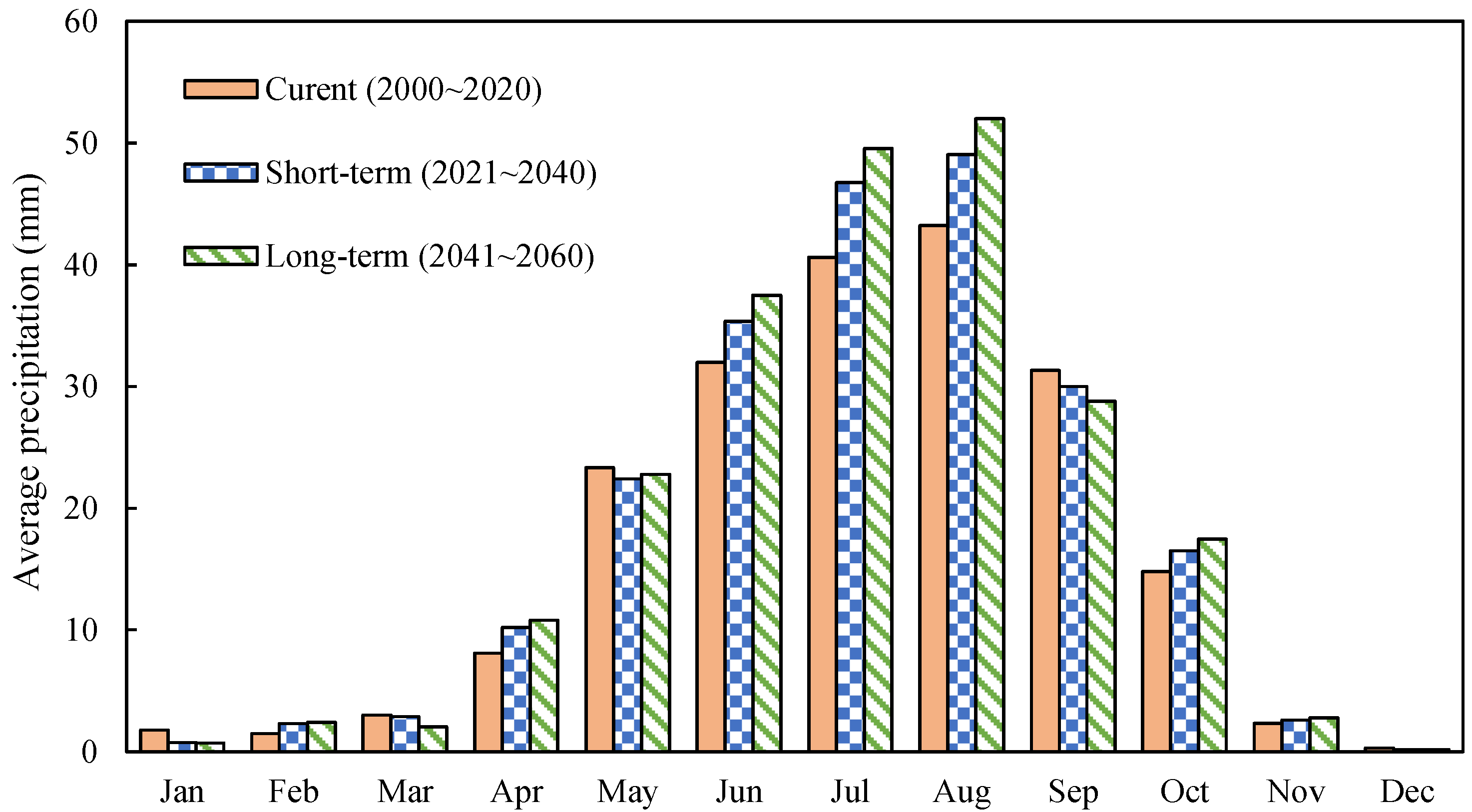
3.1.1. Change Characteristics of Precipitation

Based on the precipitation prediction results, the average precipitation in the study area is projected to be 218.9 mm for the short-term period (2021–2040) and 226.9 mm for the long-term period (2041–2060). These values are 16.7 mm and 24.7 mm higher, respectively, than the average precipitation in the current period (2001–2020), indicating an increase in annual precipitation in the study area. Figure 4 illustrates the monthly average precipitation forecast for different periods. The monthly average precipitation follows a similar trend throughout the year, with the highest amount occurring in August. This suggests that future climate changes have minimal influence on the annual distribution of precipitation. Analyzing the monthly precipitation, there is an increase in precipitation during February, April, June–August, and October–November. The largest increase is observed in July, with a short-term increase of 6.1 mm and a long-term increase of 8.9 mm. Precipitation in January, March, May, September, and December decreases, though the decrease is not significant in most months.

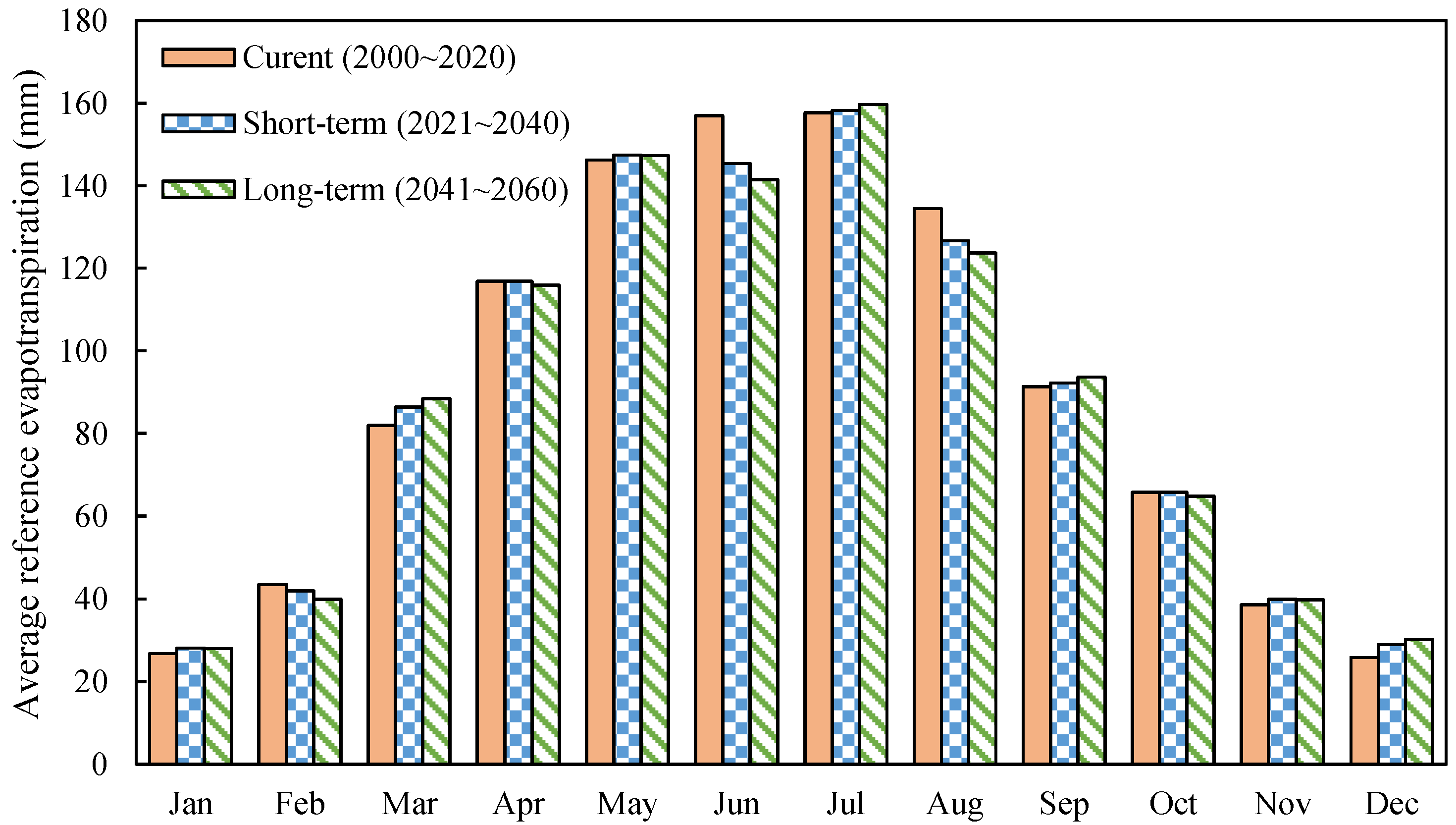
3.1.2. Change Characteristics of Reference Evapotranspiration

Based on the predicted results of reference evapotranspiration, the average reference evapotranspiration in the study area for the short-term and long-term periods is 1077.8 mm and 1072.7 mm, respectively. These values are 8.2 mm and 13.3 mm lower than the current years’ average, indicating a decline in reference evapotranspiration in the planning period. Figure 5 illustrates the monthly average reference evapotranspiration across different periods. The monthly average reference evapotranspiration for both the short-term and long-term periods follows a similar trend throughout the year, with the peak shifting from June to July. This shift suggests that future climate conditions may affect the annual distribution of reference evapotranspiration. Specifically, reference evapotranspiration has decreased in February, April, June, August, and October, with the most significant decline observed in June. The decreases in June are 11.6 mm and 15.5 mm for the short-term and long-term periods, respectively. Conversely, reference evapotranspiration has increased in January, March, May, July, September, and November to December, with increments ranging from 0.1 to 6.5 mm.

3.2. Optimal Allocation of Irrigation Water Diversion (Model I)

3.2.1. Optimization Results of Irrigation Benefits (Model I)

Figure 6 illustrates the net profit optimization results across different periods. For the current years, the optimized net profit increased from USD [41.35, 54.81] million to USD [59.62, 78.98] million, reflecting a rise of USD [18.27, 24.18] million, accompanied by a significant improvement in irrigation efficiency. In the upcoming year, the projected net profits for the short-term and long-term are estimated at USD [61.81, 81.46] million and USD [62.64, 82.42] million, respectively, representing increases of USD [2.20, 2.47] million and USD [3.02, 3.43] million compared to the current years. These gains are attributed to an increase in precipitation by 6.1 mm and 8.9 mm in the short term and long term, respectively, relative to the current years. The augmented precipitation reduces crop irrigation requirements, thereby enhancing both irrigation area and efficiency. Additionally, reference evapotranspiration decreased by 11.6 mm in the short term and by 15.5 mm in the long term, which further reduces crop water demand, subsequently lowering the crop irrigation quota and enhancing irrigation efficiency.

Water productivity refers to the net profit generated by the consumption of irrigation water per unit volume for crops and is a crucial factor in optimizing water resource allocation. Figure 7 illustrates the significant variation in water productivity across different crops. Goji berries exhibit the highest water productivity ([1.15, 1.41] USD/m³), followed by forest fruits and potatoes ([0.60, 0.81] and [0.39, 0.55] USD/m³, respectively). Spring wheat and corn have the lowest water productivity ([0.08, 0.11] and [0.06, 0.09] USD/m³, respectively).

Table 9. Results of net profit (million USD) optimization for various crops during different periods (Model I).

Crop Type	Current		Short-Term	Long-Term
	Before Optimization	After Optimization
Spring wheat	[2.26, 2.95]	[1.29, 1.68]	[1.30, 1.69]	[1.30, 1.70]
Corn	[3.34, 4.87]	[2.2, 3.22]	[2.24, 3.25]	[2.26, 3.27]
Flax	[2.27, 2.55]	[0.84, 0.94]	[2.82, 3.16]	[3.64, 4.08]
Potato	[2.79, 3.87]	[6.60, 9.18]	[6.63, 9.2]	[6.63, 9.21]
Melon	[2.34, 3.28]	[2.87, 4.03]	[2.87, 4.03]	[2.88, 4.03]
Goji berry	[8.34, 10.24]	[15.06, 18.5]	[15.08, 18.52]	[15.09, 18.53]
Forest fruits	[20.04, 26.98]	[30.81, 41.48]	[30.86, 41.54]	[30.88, 41.55]

presents the net profit optimization results for each crop across different periods. In the current years, the net profit of each crop after optimization changes significantly compared to the pre-optimization values. Specifically, the net profits of spring wheat, corn, and flax, which have lower water productivity, decrease by USD [0.98, 1.27], [1.13, 1.65], and [1.43, 1.61] million, respectively. On the other hand, the net profits of potato, melon, goji berry, and forest fruits, which have higher water productivity, increase by USD [3.82, 5.30], [0.53, 0.74], [6.72, 8.26], and [10.77, 14.50] million, respectively. The optimization results indicate that in the future years, only the net profit of flax shows a significant increase. Specifically, in the short-term and long-term future years, the net profit of flax increased by USD 0.55 to 2.80 million and USD 2.22 to 3.14 million, respectively, compared to the current years. This suggests that climate change will increase the availability of distributable irrigation water in the future, which will be allocated to expand the planting area of flax, ultimately improving the irrigation efficiency of the region.

3.2.2. Optimization Results of Crop Planting Structure (Model I)

Figure 8 illustrates the total planting area of crops across different periods. For the current years, the total planting area of crops increased from 16.5 thousand hectares before optimization to 17.4 thousand hectares after optimization, representing an increase of 0.9 thousand hectares. For the future year, the total planting area of crops is projected to be 18.1 thousand hectares in the short term and 18.4 thousand hectares in the long term, which are 0.7 and 1.0 thousand hectares more than the current years, respectively. Due to constraints on the total amount of irrigation water available, the total planting area of crops in each period does not reach the total arable land area in the irrigation region (20.01 thousand hectares). The potential increase in crop planting area for the current years, short-term years, and long-term years are 2.6, 1.9, and 1.6 thousand hectares, respectively. Despite the shortage of irrigation water resources, efficient use of return flow can lead to an expansion in crop planting area.

Table 10. Planting structure optimization results of different crops in different periods (Model I).

Crop Type	Current		Short-Term	Long-Term
	Before Optimization	After Optimization
Spring wheat	22.6%	12.2%	11.7%	11.5%
Corn	30.0%	18.8%	18.0%	17.8%
Flax	5.0%	1.8%	5.6%	7.2%
Potato	5.3%	11.9%	11.5%	11.3%
Melon	5.6%	6.5%	6.2%	6.1%
Goji berry	11.2%	19.2%	18.4%	18.1%
Forest fruits	20.4%	29.7%	28.5%	28.1%

presents the results of crop planting structure optimization for different periods. In the current years, the proportion of the planting area for each crop significantly changes compared to the pre-optimization state. Specifically, the planting proportions of spring wheat, corn, and flax, which have low water productivity, decrease by 10.4%, 11.2%, and 3.2%, respectively. Conversely, the planting proportions of potato, melon, goji berry, and forest fruit, which have high water productivity, increase by 6.6%, 0.9%, 8.0%, and 9.3%, respectively. The future year optimization results indicate that only the planting proportion of flax will increase. In the short-term future, the planting proportion of flax will rise by 3.8%, and in the long-term future, it will increase by 5.4% compared to the current optimized planting proportion. This suggests that the increase in distributable irrigation water due to future climate change will be allocated to expanding flax planting areas, thereby increasing its planting proportion.

3.2.3. Results of Optimal Allocation of Water Resources (Model I)

According to the optimized allocation results of irrigation water diversion, the total irrigation water diversion for the current years and the future years reaches the maximum allowable limit of 145 million m³ in the irrigation area. This indicates that the irrigation efficiency in the area is constrained by the total available water resources. If return flow can be fully utilized, the irrigation efficiency could be improved.

Figure 9 shows the net irrigation quota for each crop during different periods. The irrigation quota is influenced by both crop water demand and effective precipitation. The crops with irrigation quotas from largest to smallest are corn, forest fruits, flax, melon, potato, spring wheat, and goji berry. In the long term, the current irrigation quota is the highest, while the net irrigation water demand in both the short and long term gradually decreases. This is due to an increase in future precipitation and a decrease in reference evapotranspiration, leading to a reduced water demand for crop irrigation.

Figure 10 presents the optimization results of crop water allocation across different periods. Crop water allocation is influenced by the planting area and irrigation quota of each crop, resulting in significant variation among different crops. Forest fruit and corn require the most water due to their extensive planting areas and high irrigation demands. Consequently, the water allocation for these crops is substantial. In contrast, flax and melon have relatively low water allocations due to their smaller planting areas. Although goji berry has a large planting area, its water allocation remains relatively low because it has the lowest irrigation quota among all crops.

3.3. Optimal Allocation Considering Return Flow (Model II)

Considering the optimal allocation of return flow (model II), Chen [35] demonstrated that the quality of return flow in the Jingdian Irrigation District essentially meets the requirements for farmland irrigation. Therefore, these resources can be utilized for farmland irrigation to enhance the utilization rate of return flow and improve irrigation efficiency. By optimizing the allocation of return flow resources for both the current and future years, the impact of return flow reuse on irrigation efficiency, crop planting structure, and water resource allocation in irrigation areas is analyzed.

3.3.1. Optimization Results of Irrigation Benefits (Model II)

Table 11. Optimization results of total net profit (million USD) for different periods.

	Current	Short-Term	Long-Term
Ignore return flow	[59.62, 78.98]	[61.81, 81.46]	[62.64, 82.42]
Consider return flow	[66.76, 86.95]	[66.9, 87.09]	[67.03, 87.23]
Net profit growth	[7.14, 7.97]	[5.08, 5.63]	[4.4, 4.81]

presents the results of net profit optimization across different time periods. After irrigation with return flow resources, the net profits for the current years, the short-term period, and the long-term period are USD [66.76, 86.95], [66.9, 87.09], and [67.03, 87.23] million, respectively. These figures represent increases of USD [7.14, 7.97], [5.08, 5.63], and [4.4, 4.81] million when compared to net profits without return flow. The growth of net profit diminishes from the current years to the future years, as the potential for increasing crop planting area is higher in the current years (2.6 thousand ha) compared to the future years (1.9 thousand ha in the short term and 1.6 thousand ha in the long term). Once the return flow resources are fully utilized, the irrigation area reaches its maximum capacity, leading to a decrease in net profit growth in the planning years.

Table 12. Results of net profit (million USD) optimization for various crops during different periods (Model II).

Crop Type	Current		Short-Term		Long-Term
	Ignore Return Flow	Consider Return Flow	Ignore Return Flow	Consider Return Flow	Ignore Return Flow	Consider Return Flow
Spring wheat	[1.29, 1.68]	[1.29, 1.68]	[1.30, 1.69]	[1.30, 1.69]	[1.30, 1.70]	[1.30, 1.70]
Corn	[2.2, 3.22]	[2.21, 3.23]	[2.24, 3.25]	[2.25, 3.27]	[2.26, 3.27]	[2.27, 3.28]
Flax	[0.84, 0.94]	[7.89, 8.84]	[2.82, 3.16]	[7.91, 8.87]	[3.64, 4.08]	[7.92, 8.88]
Potato	[6.6, 9.18]	[6.6, 9.18]	[6.63, 9.2]	[6.63, 9.2]	[6.63, 9.21]	[6.63, 9.21]
Melon	[2.87, 4.03]	[2.87, 4.03]	[2.87, 4.03]	[2.87, 4.03]	[2.88, 4.03]	[2.88, 4.03]
Goji berry	[15.06, 18.5]	[15.06, 18.5]	[15.08, 18.52]	[15.08, 18.52]	[15.09, 18.53]	[15.09, 18.53]
Forest fruits	[30.81, 41.48]	[30.81, 41.48]	[30.86, 41.54]	[30.86, 41.54]	[30.88, 41.55]	[30.88, 41.55]

presents the results of crop net profit optimization across different periods. It is observed that only the net profits of corn and flax increase after irrigation using return flow resources, while the net profits of other crops remain unchanged. This is because the water productivity of corn and flax is high, and the return flow resources are preferentially allocated to crops with higher water productivity to enhance irrigation efficiency.

3.3.2. Optimization Results of Crop Planting Structure (Model II)

Figure 11 presents the optimization results of the total planting area across different periods. After utilizing return flow resources for irrigation, the total planting area in each period reached a maximum of 20 thousand ha. Specifically, the total planting area increased by 2.6 thousand ha in the current years, 1.9 thousand ha in the short-term years, and 160 ha in the long-term years. Reasonable utilization of return flow resources enhances the efficiency of cultivated land in irrigation areas.

Table 13. Planting structure optimization results of different crops in different periods (Model II).

Crop Type	Current		Short-Term		Long-Term
	Ignore Return Flow	Consider Return Flow	Ignore Return Flow	Consider Return Flow	Ignore Return Flow	Consider Return Flow
Spring wheat	12.2%	10.6%	11.7%	10.6%	11.5%	10.6%
Corn	18.8%	16.4%	18.0%	16.4%	17.8%	16.4%
Flax	1.8%	14.3%	5.6%	14.3%	7.2%	14.3%
Potato	11.9%	10.4%	11.5%	10.4%	11.3%	10.4%
Melon	6.5%	5.6%	6.2%	5.6%	6.1%	5.6%
Goji berry	19.2%	16.7%	18.4%	16.7%	18.1%	16.7%
Forest fruits	29.7%	25.9%	28.5%	25.9%	28.1%	25.9%

illustrates the optimization results of crop planting structure across different periods. The crop planting proportions for the current and future years remain the same after irrigation using return flow resources. This is because the planting area in the irrigation region has reached its maximum capacity and the irrigation water resources are fully utilized, resulting in no variation in optimization outcomes. When compared to the crop planting structure without considering return flow, the planting proportion of flax increased by 12.5%, 8.7%, and 7.1% in the current years, the short-term years, and the long-term years, respectively, after considering return flow.

3.3.3. Results of Optimal Allocation of Water Resources (Model II)

Table 14. Optimization results of irrigation water in different periods (10⁶ m³).

Period	Ignore Return Flow	Consider Return Flow			Reduction of Irrigation Diversion
	Irrigation Diversion	Total Water Volume	Irrigation Diversion	Return Flow
Current	145	170	[127, 133]	[37, 43]	[12, 18]
Short-term	145	162	[121, 127]	[35, 41]	[18, 24]
Long-term	145	159	[119, 125]	[34, 40]	[20, 26]

presents the optimization results of irrigation water resources across different periods. When return flow resources are utilized for irrigation, the total water allocation for the current, short-term, and long-term years is 170, 162, and 159 million m³, respectively. This represents an increase of 25, 17, and 14 million m³ compared to the total water allocation without considering return flow. After reusing return flow resources, the irrigation diversion water allocation for the current, short-term, and long-term years ranges from [127, 133], [121, 127], and [119, 125] million m³, respectively. These allocations are [12, 18], [18, 24], and [20, 26] million m³ less than the irrigation diversion without considering return flow.

Table 15. Results of water allocation optimization for various crops during different periods (10⁶ m³).

Crop Type	Current		Short-Term		Long-Term
	Ignore Return Flow	Consider Return Flow	Ignore Return Flow	Consider Return Flow	Ignore Return Flow	Consider Return Flow
Spring wheat	15.90	15.90	15.40	15.40	15.18	15.18
Corn	35.34	35.51	33.73	33.90	33.13	33.29
Flax	2.95	27.61	9.49	26.60	12.03	26.16
Potato	16.73	16.73	15.77	15.77	15.43	15.43
Melon	9.57	9.57	9.31	9.31	9.19	9.19
Goji berry	13.12	13.12	12.08	12.08	11.67	11.67
Forest fruits	51.40	51.40	49.20	49.20	48.36	48.36

shows the optimization results of water allocation for crops over different periods. Only the water allocation for corn and flax has increased after utilizing return flow resources, while the water allocation for other crops remains unchanged. This is because corn and flax have high water productivity, and return flow resources are prioritized for crops with high water productivity to enhance irrigation efficiency.

In conclusion, utilizing return flow resources for farmland irrigation offers multiple benefits. It increases the amount of irrigation water available, improves efficiency, and avoids negative impacts on the Yellow River’s water ecological environment. Additionally, it reduces the amount of water diverted from the Yellow River, conserves water resources, and lowers the power costs associated with irrigation and water extraction.

Currently, some scholars are researching the optimization of water resources and surplus energy in irrigation systems [36]. The primary focus of optimal water resource allocation in irrigation areas is on upstream river inflow and groundwater [37], with insufficient research on the optimal allocation of return flow resources. Numerous factors affect return flow in irrigation areas, leading to uncertainty in the return flow coefficient and the amount of return flow. Using a deterministic model for optimization diminishes the reference value of the allocation results [38]. This paper incorporates return flow into the optimal allocation model, describing its uncertainty using interval numbers. Subsequently, the optimal allocation of irrigation water resources is achieved through an interval linear programming model. The results demonstrate that the uncertainty in the optimal allocation of return flow can be more effectively addressed using the interval linear programming model.

4. Conclusions

Based on the prediction of future climate change characteristics in the study area, the goal is to maximize net profit while considering the constraints of maximum irrigation diversion and maximum planting area. An uncertain water resources optimal allocation model is established, incorporating the reuse of return flow. The main conclusions are as follows:

(1)

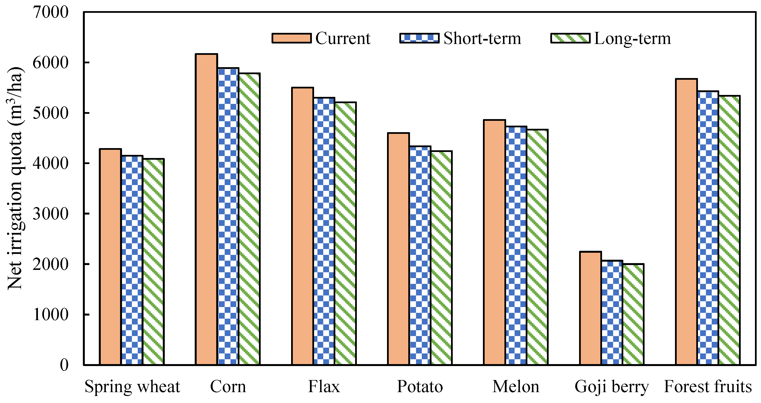
The precipitation in the study area shows an increasing trend. The annual precipitation in the short-term years and long-term years increases by 6.1 mm and 8.9 mm, respectively. The reference evapotranspiration showed a decreasing trend. The reference evapotranspiration in the short-term years and long-term years decreases by 8.2 mm and 13.3 mm respectively.

(2)

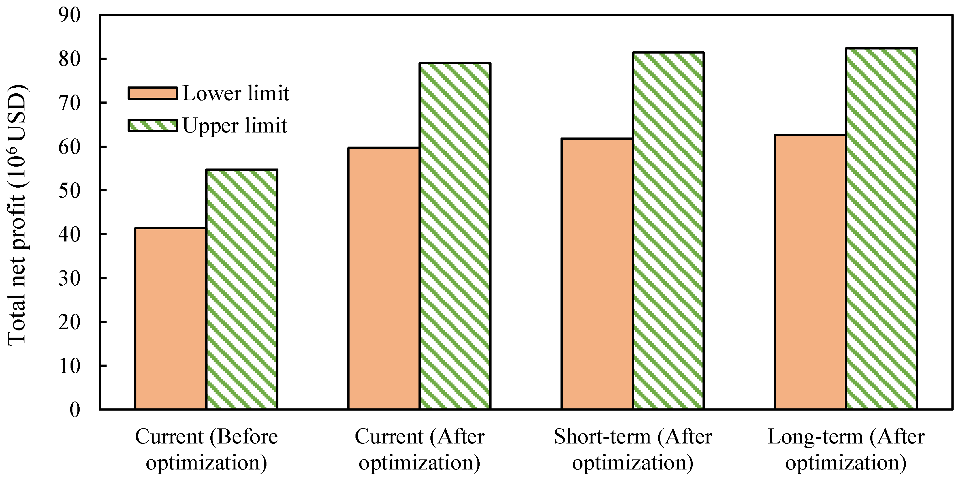
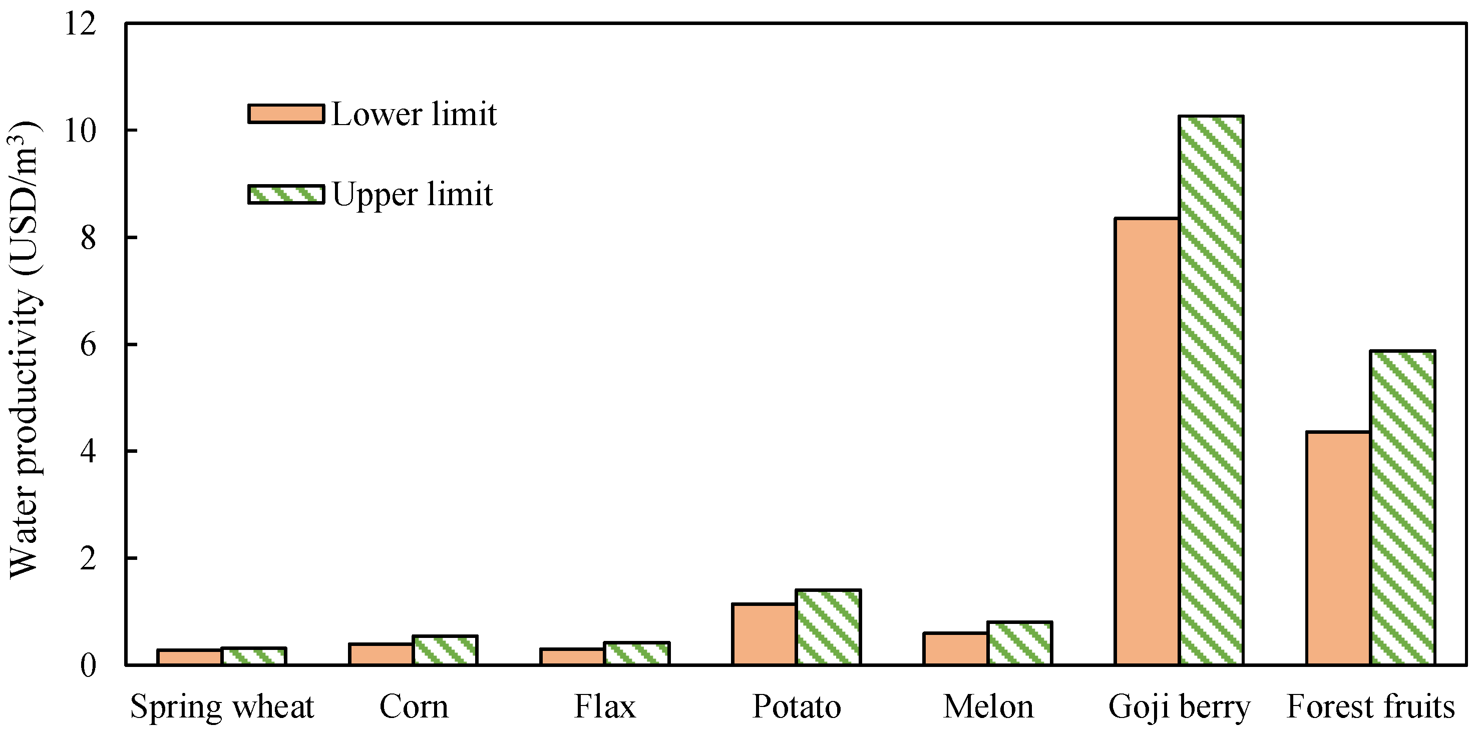
After optimizing the optimal allocation of irrigation water diversion (model I) in the current years, the net profit increased by USD [18.27, 24.18] million, and the total planting area increased by 900 ha. The crop planting structure changes significantly, with a decrease in the planting proportion of low water productivity crops (spring wheat, corn, and flax) and an increase in the planting proportion of high water productivity crops (potato, melon, goji berry, and forest fruits). After optimizing for the upcoming years, the net profit for both the short-term and long-term years saw an increase of USD [2.20, 2.47] and [3.02, 3.43] million respectively. Additionally, the total planting area expands by 700 hectares and 1000 hectares respectively. Due to limitations in irrigation water diversion, the irrigation area faces a shortage of water resources. However, there is potential to increase the crop planting area in both the current years and the planning years. By effectively utilizing the return flow, the crop planting area can be expanded even further.

(3)

When optimizing the allocation of return flow (model II), the net profit of the current years, short-term years, and the long-term years increased by USD [7.14, 7.97], [5.08, 5.63] and [4.4, 4.81] million, respectively, compared with the net profit of model I. The total planting area also increased by 2.6 thousand ha, 1.9 thousand ha, and 1.6 thousand ha, respectively, compared with the total planting area of model I. Additionally, the amount of irrigation water diversion was reduced by [12, 18] million m³, [18, 24] million m³, and [20, 26] million m³, respectively, compared with that of model I. The use of return flow resources for farmland irrigation can not only improve irrigation efficiency and avoid the pollution of return flow discharge on the water quality of the Yellow River, but also reduce water diversion from the Yellow River, play a water-saving role, and reduce the cost of water extraction to a certain extent.

(4)

The application of interval linear programming models can effectively optimize the allocation of irrigation return flow under conditions of uncertainty. This study also serves as a reference for the reuse and optimization of irrigation return flow in other arid regions, contributing positively to the efficient utilization of water resources and the protection of water environments. In addition to irrigation return flow, the method proposed in this study can also be applied for the optimal allocation of the reuse of treated industrial and domestic wastewater. However, it is important to determine a reasonable interval number as a constraint condition.

References

1. Ren, C.; Li, Z.; Zhang, H. Integrated multi-objective stochastic fuzzy programming and AHP method for agricultural water and land optimization allocation under multiple uncertainties. J. Clean. Prod. 2019, 210, 12–24. [Google Scholar] [CrossRef]
2. Zhuang, X.W.; Li, Y.P.; Nie, S.; Fan, Y.R.; Huang, G.H. Analyzing climate change impacts on water resources under uncertainty using an integrated simulation-optimization approach. J. Hydrol. 2018, 556, 523–538. [Google Scholar] [CrossRef]
3. Zhang, J.X.; Deng, M.J.; Li, P.; Li, Z.B.; Huang, H.P.; Shi, P.; Feng, C.H. Security pattern and regulation of agricultural water resources in Northwest China from the perspective of virtual water flow. Strateg. Study CAE 2022, 24, 131–140. [Google Scholar] [CrossRef]
4. Song, W. The Research on Runoff Evolution and Allocation of Water Resources in the Area of Qianzhong Water Diversion Project. Master’s Thesis, Tianjin University, Tianjin, China, 2016. [Google Scholar]
5. Gao, Z. Progresses and challenges in the study of Eco-fluvial dynamics. J. Hydraul. Eng. 2019, 50, 88–96. [Google Scholar]
6. Shi, Y.W. Study on the Regularity of Drainage Water Volume of Qingtongxia Irrigation Area of Ningxia. Master’s Thesis, Xi’an University of Technology, Xi’an, China, 2005. [Google Scholar]
7. Li, J.; Song, J.; Li, M.; Shang, S.; Mao, X.; Yang, J.; Adeloye, A.J. Optimization of irrigation scheduling for spring wheat based on simulation-optimization model under uncertainty. Agric. Water Manag. 2018, 208, 245–260. [Google Scholar] [CrossRef]
8. Li, M.; Jiang, Y.; Guo, P.; Li, J. Irrigation water optimal allocation considering stakeholders of different levels. Trans. Chin. Soc. Agric. Mach. 2017, 48, 199–207. [Google Scholar]
9. Montazar, A.; Riazi, H.; Behbahani, S.M. Conjunctive water use planning in an irrigation command area. Water Resour. Manag. 2010, 24, 577–596. [Google Scholar] [CrossRef]
10. Feng, J. Optimal allocation of regional water resources based on multi-objective dynamic equilibrium strategy. Appl. Math. Model. 2021, 90, 1183–1203. [Google Scholar] [CrossRef]
11. Habibi, D.M.; Banihabib, M.E.; Nadjafzadeh, A.A.; Hashemi, S.R. Multi-objective optimization model for the allocation of water resources in arid regions based on the maximization of socioeconomic efficiency. Water Resour. Manag. 2016, 30, 927–946. [Google Scholar] [CrossRef]
12. Afzal, J.; Noble, D.H.; Weatherhead, E.K. Optimization model for alternative use of different quality irrigation waters. J. Irrig. Drain. Eng. 1992, 118, 218–228. [Google Scholar] [CrossRef]
13. Guo, P.; Chen, X.; Li, M.; Li, J. Fuzzy chance-constrained linear fractional programming approach for optimal water allocation. Stoch. Environ. Res. Risk Assess. 2013, 28, 1601–1612. [Google Scholar] [CrossRef]
14. Yang, G.Q.; Guo, P.; Li, R.H.; Li, M. Optimal allocation model of surface water and groundwater based on queuing theory in irrigation district. Trans. Chin. Soc. Agric. Eng. 2016, 32, 115–120. [Google Scholar]
15. Cui, L.; Li, Y.; Huang, G. Double-sided fuzzy chance-constrained linear fractional programming approach for water resources management. Eng. Optim. 2016, 48, 949–965. [Google Scholar] [CrossRef]
16. Karamouz, M.; Kerachian, R.; Zahraie, B. Monthly water resources and irrigation planning: Case study of conjunctive use of surface and groundwater resources. J. Irrig. Drain. Eng. 2004, 130, 391–402. [Google Scholar] [CrossRef]
17. Bazargan-Lari, M.R.; Kerachian, R.; Mansoori, A. A conflict-resolution model for the conjunctive use of surface and groundwater resources that considers water-quality issues: A case study. Environ. Manag. 2009, 43, 470–482. [Google Scholar] [CrossRef] [PubMed]
18. Zhang, Z.X. Multi-Water Conjunctive Optimal Allocation Model of Irrigation Area Research Under Uncertainty. Master’s Thesis, Northeast Agricultural University, Harbin, China, 2016. [Google Scholar]
19. Zhang, C.; Guo, P.; Huo, Z. Irrigation water resources management under uncertainty: An interval nonlinear double-sided fuzzy chance-constrained programming approach. Agric. Water Manag. 2021, 245, 106658. [Google Scholar] [CrossRef]
20. Maqsood, I.; Huang, G.; Huang, Y.; Chen, B. ITOM: An interval-parameter two-stage optimization model for stochastic planning of water resources systems. Stoch. Environ. Res. Risk Assess. 2005, 19, 125–133. [Google Scholar] [CrossRef]
21. Fu, Q.; Li, J.H.; Liu, D.; Li, T.X. Allocation optimization of water resources based on uncertainty stochastic programming model considering risk value. Trans. Chin. Soc. Agric. Eng. 2016, 32, 136–144. [Google Scholar]
22. Huang, Y.; Li, Y.P.; Chen, X.; Ma, Y.G. Optimization of the irrigation water resources for agricultural sustainability in Tarim River Basin, China. Agric. Water Manag. 2012, 107, 74–85. [Google Scholar] [CrossRef]
23. Yang, G.; Guo, P.; Huo, L.; Ren, C. Optimization of the irrigation water resources for Shijin irrigation district in north China. Agric. Water Manag. 2015, 158, 82–98. [Google Scholar] [CrossRef]
24. Li, M.; Guo, P.; Singh, V.P. Biobjective optimization for efficient irrigation under fuzzy uncertainty. J. Irrig. Drain. Eng. 2016, 142, 05016003. [Google Scholar] [CrossRef]
25. Wang, Y.; Liu, L.; Ping, G.; Zhang, C.; Fan, Z.; Guo, S. An inexact irrigation water allocation optimization model under future climate change. Stoch. Environ. Res. Risk Assess. 2019, 33, 271–285. [Google Scholar] [CrossRef]
26. Yue, Q.; Zhang, F.; Zhang, C.; Zhu, H.; Tang, Y.; Guo, P. A full fuzzy-interval credibility-constrained nonlinear programming approach for irrigation water allocation under uncertainty. Agric. Water Manag. 2020, 230, 105961. [Google Scholar] [CrossRef]
27. Guo, S.; Zhang, F.; Zhang, C.; An, C.; Wang, S.; Guo, P. A multi-objective hierarchical model for irrigation scheduling in the complex canal system. Sustainability 2018, 11, 24. [Google Scholar] [CrossRef]
28. Gong, X.; Zhang, H.; Ren, C.; Sun, D.; Yang, J. Optimization allocation of irrigation water resources based on crop water requirement under considering effective precipitation and uncertainty. Agric. Water Manag. 2020, 239, 106264. [Google Scholar] [CrossRef]
29. Yan, W.B.; Yu, L.H.; Cheng, H.Z. Simulation and prediction of future precipitation and temperature change in Poyang Lake Basin—Based on the SDSM statistical downscaling method. China Rural. Water Hydropower 2015, 7, 36–43. [Google Scholar]
30. Feng, Y.; Cui, N.B.; Gong, D.Z.; Wei, X.P. Projection of reference evapotranspiration in hilly area of central Sichuan using statistical downscaling model. Trans. Chin. Soc. Agric. Eng. 2016, 31 (Suppl. S1), 71–79. [Google Scholar]
31. Li, Q.Q.; Li, Y.P.; Huang, G.H.; Wang, C.X. Risk aversion based interval stochastic programming approach for agricultural water management under uncertainty. Stoch. Environ. Res. Risk Assess. 2017, 32, 715–732. [Google Scholar] [CrossRef]
32. Guo, S.; Zhang, F.; Zhang, C.; Wang, Y.; Guo, P. An improved intuitionistic fuzzy interval two-stage stochastic programming for resources planning management integrating recourse penalty from resources scarcity and surplus. J. Clean. Prod. 2019, 234, 185–199. [Google Scholar] [CrossRef]
33. Zhang, F.; Zhang, C.; Yan, Z.; Guo, S.; Wang, Y.; Guo, P. An interval nonlinear multiobjective programming model with fuzzy-interval credibility constraint for crop monthly water allocation. Agric. Water Manag. 2018, 209, 123–133. [Google Scholar] [CrossRef]
34. Huang, G.H.; Baetz, B.W.; Patry, G.G. A grey fuzzy linear programming approach for municipal solid waste management planning under uncertainty. Civ. Eng. Syst. 1993, 10, 123–146. [Google Scholar] [CrossRef]
35. Chen, N.S. Study on the Prediction of Return Water and the Temporal and Spatial Variation Characteristics of Water Quality in Large-Scale Yellow River Diversion Irrigation Area. Master’s Thesis, Xi’an University of Technology, Xi’an, China, 2021. [Google Scholar]
36. Rodríguez-Pérez, A.M.; Rodríguez-Gonzalez, C.A.; López, R.; Hernández-Torres, J.A.; Caparrós-Mancera, J.J. Water Microturbines for Sustainable Applications: Optimization Analysis and Experimental Validation. Water Resour. Manag. 2024, 38, 1011–1025. [Google Scholar] [CrossRef]
37. Zhao, M.; Guo, P.; Zhang, Y. Study on the water optimal allocation in irrigation district based on considering soil water balance. J. China Agric. Univ. 2020, 25, 91–102. [Google Scholar]
38. Fu, Y.H.; Guo, P.; Fang, S.Q. Optimal water resources planning based on interval-parameter two-stage stochastic programming. Trans. Chin. Soc. Agric. Eng. 2014, 30, 73–81. [Google Scholar]
Figure 1. Location map of the study area.
Applsci 15 02380 g001
Figure 2. Meteorological element diagram of the study area.
Applsci 15 02380 g002
Figure 3. Flowchart of optimal allocation.
Applsci 15 02380 g003
Figure 4. Prediction of the monthly average precipitation in different periods.
Applsci 15 02380 g004
Figure 5. Prediction of the monthly average reference evapotranspiration in different periods.
Applsci 15 02380 g005
Figure 6. Optimization results for net profit in different periods.
Applsci 15 02380 g006
Figure 7. Water productivity of different crops.
Applsci 15 02380 g007
Figure 8. Total planting area in different periods.
Applsci 15 02380 g008
Figure 9. Net irrigation quota of different crops in different periods.
Applsci 15 02380 g009
Figure 10. Water allocation optimization results for various crops during different periods.
Applsci 15 02380 g010
Figure 11. Total planting area optimization results in different periods.
Applsci 15 02380 g011