
A Local Discrete Feature Histogram for Point Cloud Feature Representation


Abstract
1. Introduction
2. Literature Review
3. Methods
3.1. LRF and LMA
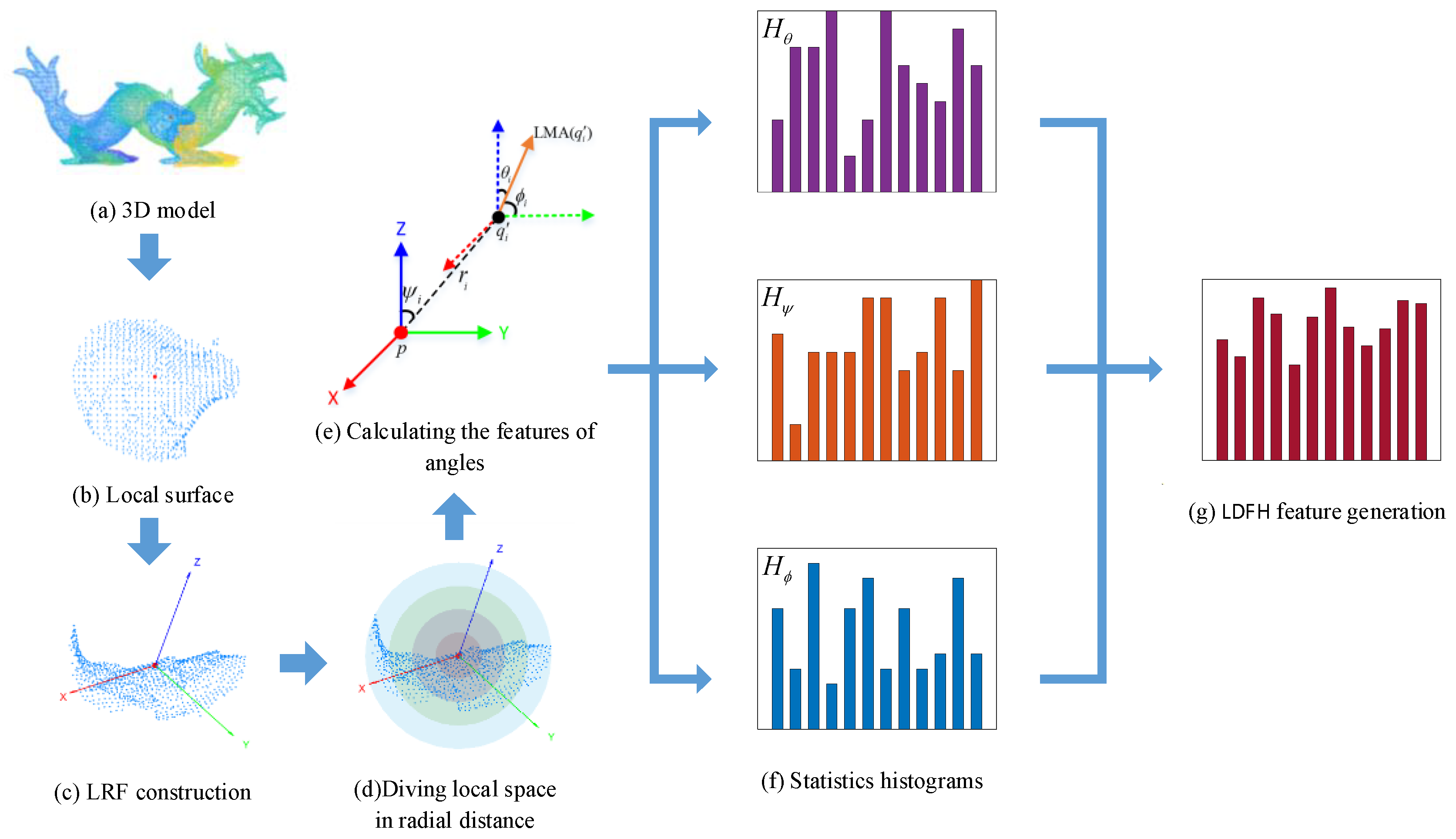
3.2. Generation of the LDFH Descriptor
| Algorithm 1: LDFH Descriptor Generation |
| Input: P (Point Cloud), K (Key Points), R, , , LRF, LMA |
| Output: LDFH (LDFH descriptors) |
| 1. For each key point, ∈ K: |
| 2. Extract local surface around the key point ; |
| 3. Construct LRF at the key point ; |
| 4. Transform local surface of to LRF; |
| 5. Partition local space around into radial bins ; |
| 6. For each neighboring point in support radius: |
| 7. Compute geometric attributes based on LRF; |
| 8. Generate three feature histograms ; |
| 9. Apply a weighted fusion to generate the final LDFH descriptor ; |
| 10. Store the LDFH descriptor for key point ; |
| 11. Return LDFH (set of all LDFH descriptors for K). |
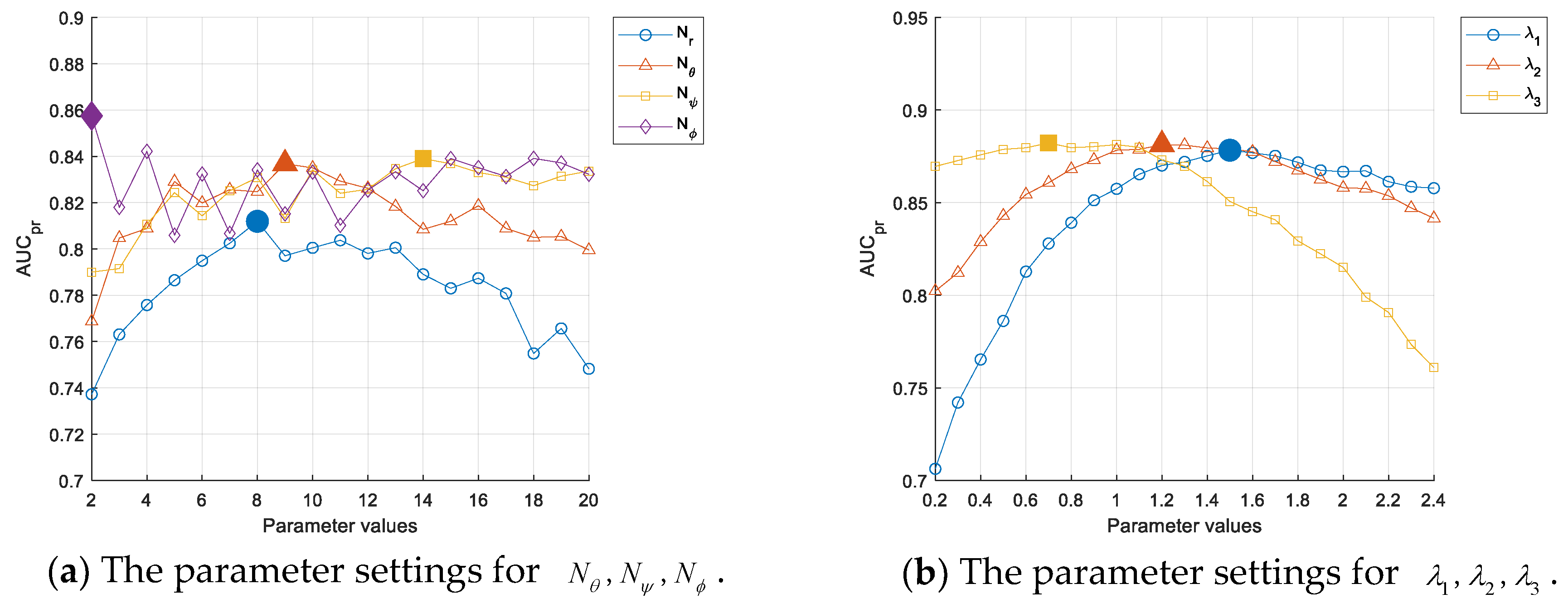
3.3. Parameter Settings
4. Experimental Results
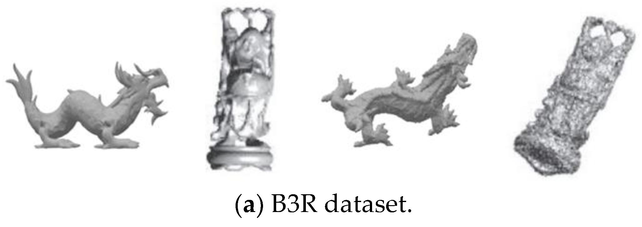
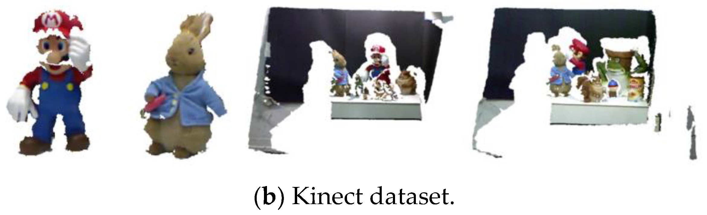
4.1. Datasets
4.2. Evaluation Criteria
4.3. Performance Evaluation of the LDFH Descriptor
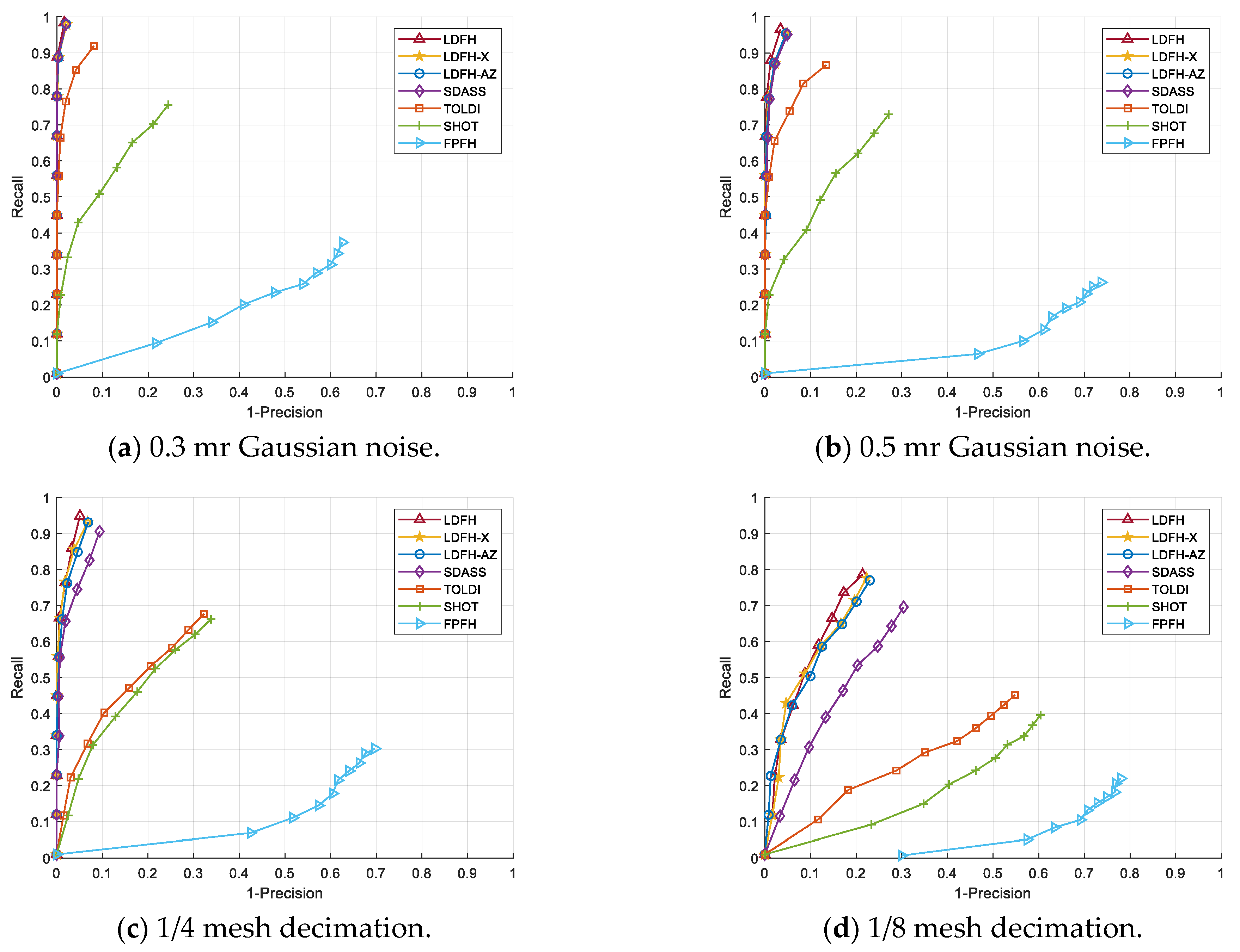
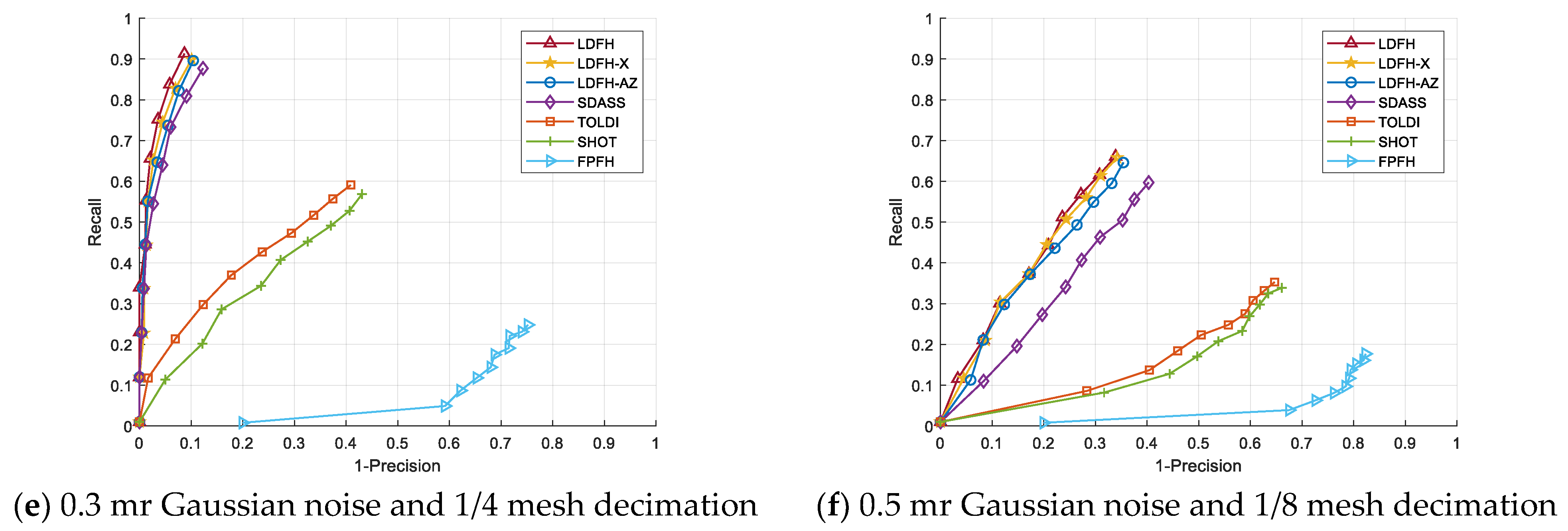
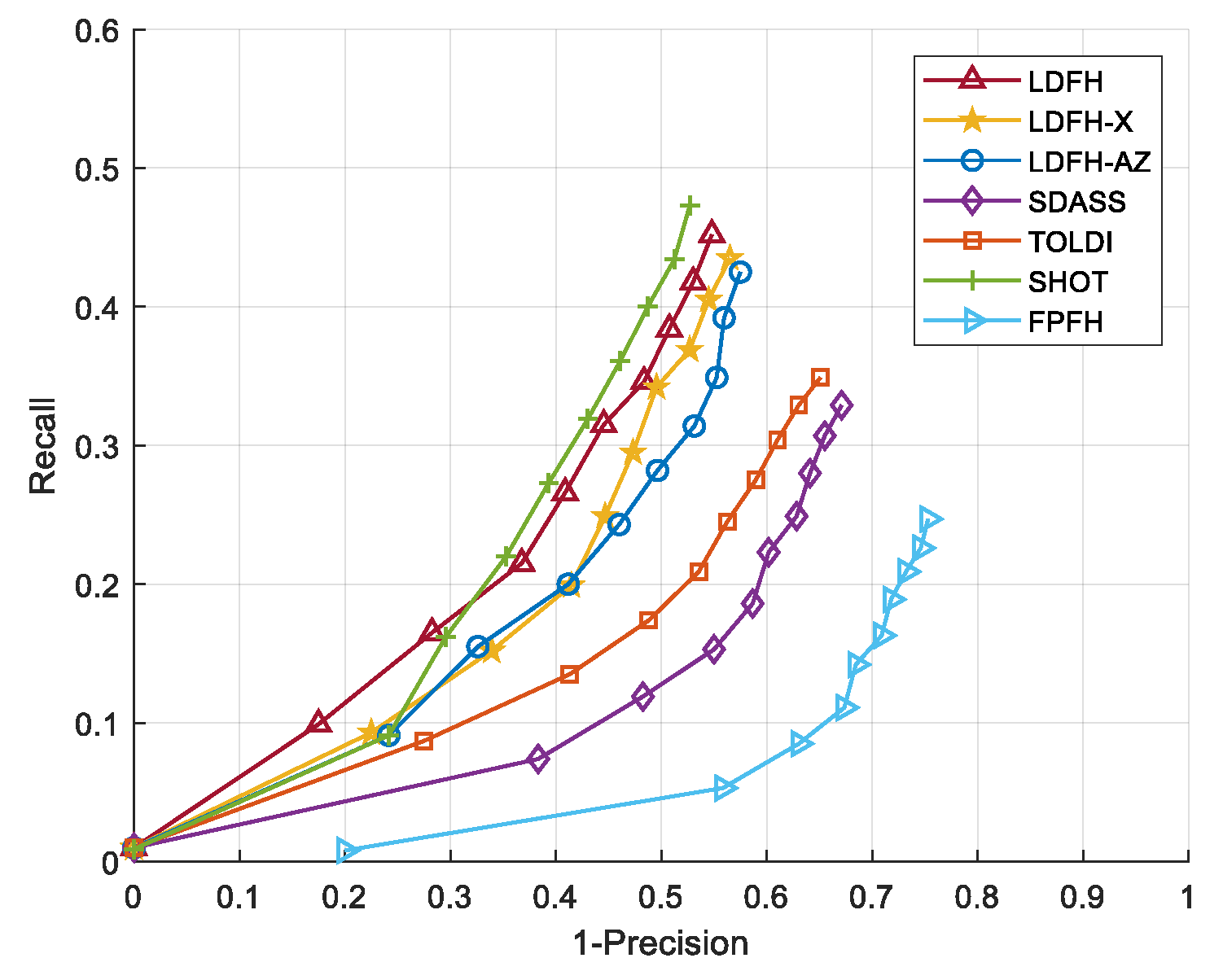
4.3.1. Descriptiveness and Robustness
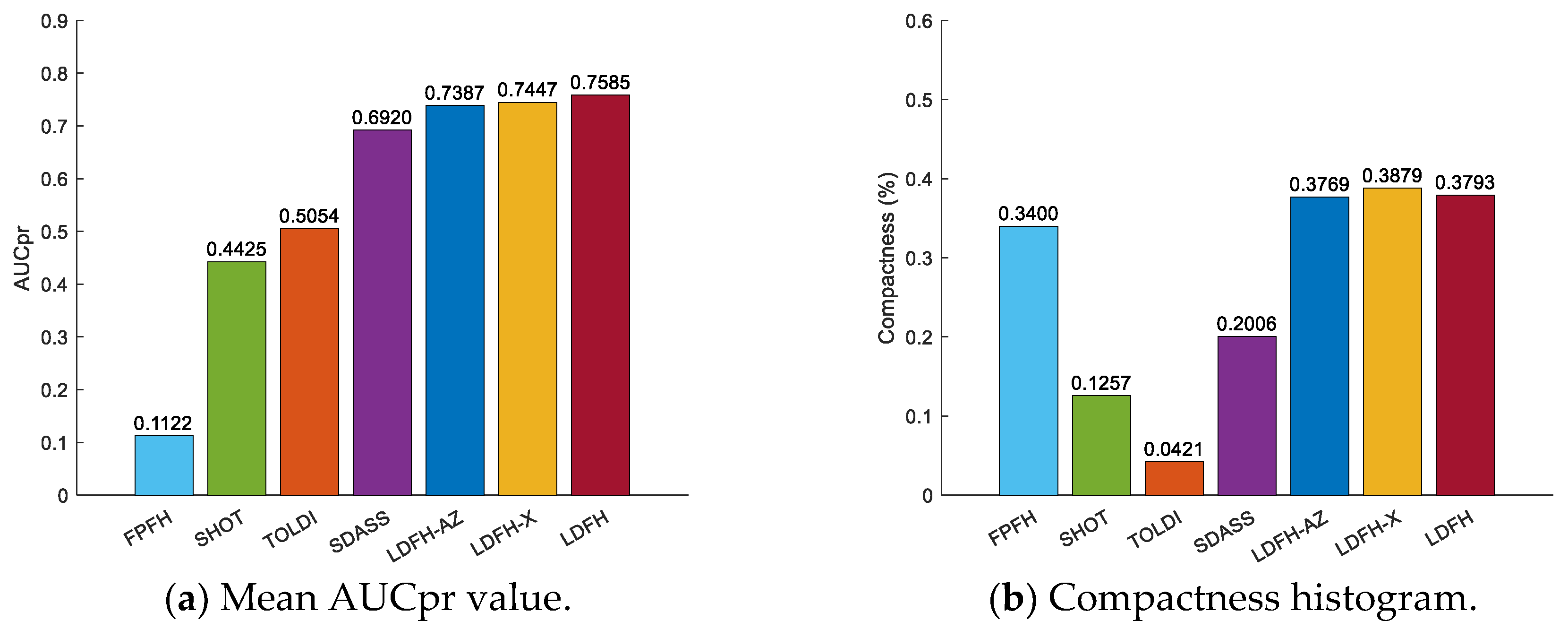
4.3.2. Compactness
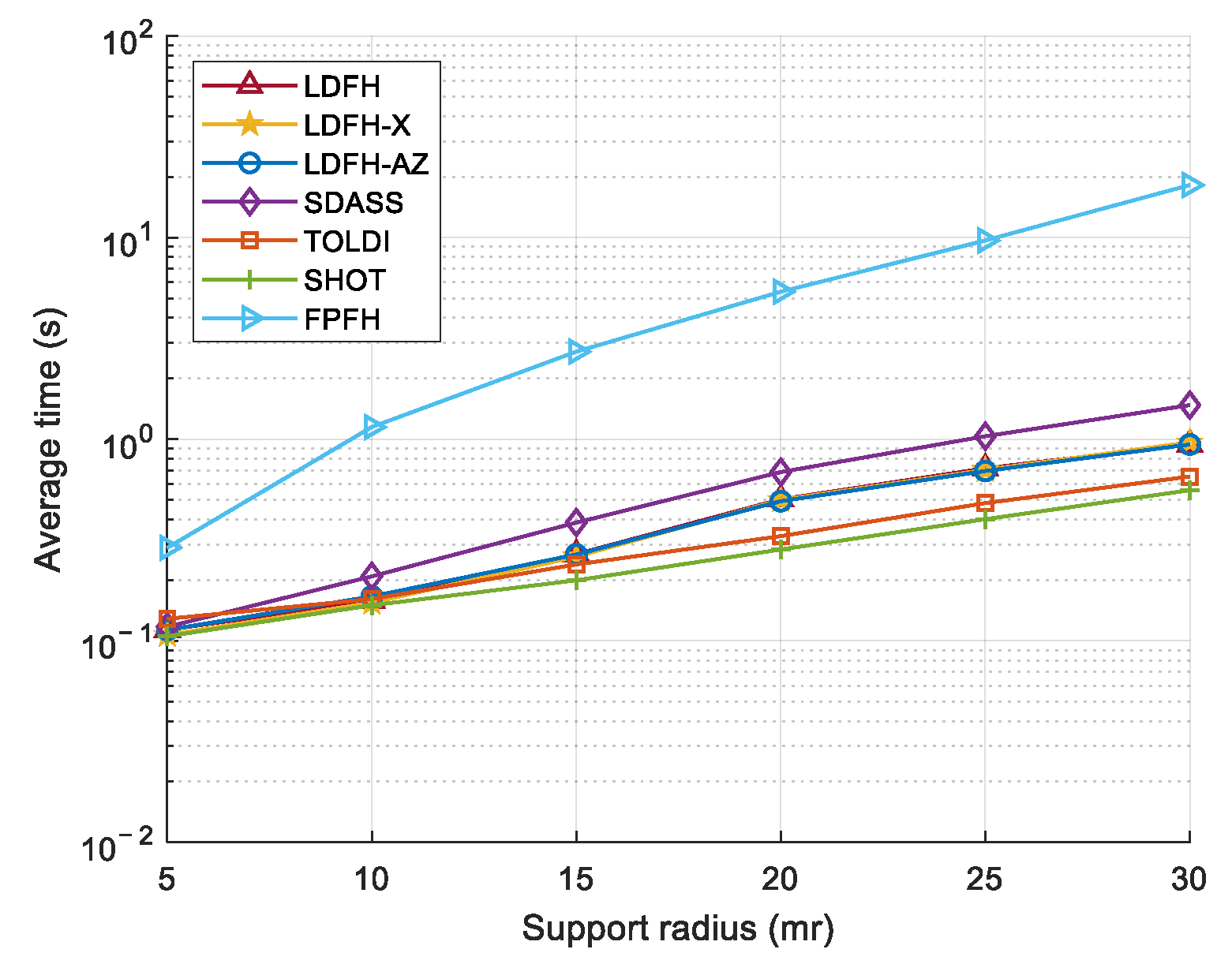
4.3.3. Efficiency
5. Conclusions
Author Contributions
Funding
Data Availability Statement
Acknowledgments
Conflicts of Interest
References
- Yan, H.; Zhang, J.X.; Zhang, X. Injected Infrared and Visible Image Fusion via L1 Decomposition Model and Guided Filtering. IEEE Trans. Comput. Imaging 2022, 8, 162–173. [Google Scholar] [CrossRef]
- Zhang, X.; Liu, R.; Ren, J.; Gui, Q. Adaptive fractional image enhancement algorithm based on rough set and particle swarm optimization. Fractal Fract. 2022, 6, 100. [Google Scholar] [CrossRef]
- Dong, Z.; Liang, F.X.; Yang, B.S.; Xu, Y.S.; Zang, Y.F.; Li, J.P.; Wang, Y.; Dai, W.X.; Fan, H.C.; Hyyppä, J.; et al. Registration of large-scale terrestrial laser scanner point clouds: A review and benchmark. ISPRS-J. Photogramm. Remote Sens. 2020, 163, 327–342. [Google Scholar] [CrossRef]
- Yang, J.Q.; Cao, Z.G.; Zhang, Q. A fast and robust local descriptor for 3D point cloud registration. Inf. Sci. 2016, 346, 163–179. [Google Scholar] [CrossRef]
- Mian, A.S.; Bennamoun, M.; Owens, R. Three-dimensional model-based object recognition and segmentation in cluttered scenes. IEEE Trans. Pattern Anal. Mach. Intell. 2006, 28, 1584–1601. [Google Scholar] [CrossRef]
- Guo, Y.L.; Bennamoun, M.; Sohel, F.; Lu, M.; Wan, J.W. 3D Object Recognition in Cluttered Scenes with Local Surface Features: A Survey. IEEE Trans. Pattern Anal. Mach. Intell. 2014, 36, 2270–2287. [Google Scholar] [CrossRef]
- Bronstein, A.M.; Bronstein, M.M.; Guibas, L.J.; Ovsjanikov, M. Shape Google: Geometric Words and Expressions for Invariant Shape Retrieval. ACM Trans. Graph. 2011, 30, 20. [Google Scholar] [CrossRef]
- Gao, Y.; Dai, Q.H. View-Based 3D Object Retrieval: Challenges and Approaches. IEEE Multimed. 2014, 21, 52–57. [Google Scholar] [CrossRef]
- Guo, Y.L.; Bennamoun, M.; Sohel, F.; Lu, M.; Wan, J.W.; Kwok, N.M. A Comprehensive Performance Evaluation of 3D Local Feature Descriptors. Int. J. Comput. Vis. 2016, 116, 66–89. [Google Scholar] [CrossRef]
- Yang, J.Q.; Xiao, Y.; Cao, Z.G. Toward the Repeatability and Robustness of the Local Reference Frame for 3D Shape Matching: An Evaluation. IEEE Trans. Image Process. 2018, 27, 3766–3781. [Google Scholar] [CrossRef]
- Ghorbani, F.; Ebadi, H.; Sedaghat, A.; Pfeifer, N. A Novel 3-D Local DAISY-Style Descriptor to Reduce the Effect of Point Displacement Error in Point Cloud Registration. IEEE J. Sel. Top. Appl. Earth Observ. Remote Sens. 2022, 15, 2254–2273. [Google Scholar] [CrossRef]
- Yang, J.Q.; Quan, S.W.; Wang, P.; Zhang, Y.N. Evaluating Local Geometric Feature Representations for 3D Rigid Data Matching. IEEE Trans. Image Process. 2020, 29, 2522–2535. [Google Scholar] [CrossRef] [PubMed]
- Tombari, F.; Salti, S.; Di Stefano, L. Unique signatures of histograms for local surface description. In Proceedings of the Computer Vision–ECCV 2010: 11th European Conference on Computer Vision, Heraklion, Crete, Greece, 5–11 September 2010; Proceedings, Part III 11. pp. 356–369. [Google Scholar]
- Guo, Y.L.; Sohel, F.; Bennamoun, M.; Lu, M.; Wan, J.W. Rotational Projection Statistics for 3D Local Surface Description and Object Recognition. Int. J. Comput. Vis. 2013, 105, 63–86. [Google Scholar] [CrossRef]
- Yang, J.Q.; Zhang, Q.; Xiao, Y.; Cao, Z.G. TOLDI: An effective and robust approach for 3D local shape description. Pattern Recognit. 2017, 65, 175–187. [Google Scholar] [CrossRef]
- Du, Z.H.; Zuo, Y.; Qiu, J.F.; Li, X.; Li, Y.; Guo, H.X.; Hong, X.B.; Wu, J. MDCS with fully encoding the information of local shape description for 3D Rigid Data matching. Image Vis. Comput. 2022, 121, 104421. [Google Scholar] [CrossRef]
- Liu, X.S.; Li, A.H.; Sun, J.F.; Lu, Z.Y. Trigonometric projection statistics histograms for 3D local feature representation and shape description. Pattern Recognit. 2023, 143, 109727. [Google Scholar] [CrossRef]
- Shi, C.H.; Wang, C.Y.; Liu, X.L.; Sun, S.Y.; Xi, G.; Ding, Y.Y. Point cloud object recognition method via histograms of dual deviation angle feature. Int. J. Remote Sens. 2023, 44, 3031–3058. [Google Scholar] [CrossRef]
- Zhao, B.; Le, X.Y.; Xi, J.T. A novel SDASS descriptor for fully encoding the information of a 3D local surface. Inf. Sci. 2019, 483, 363–382. [Google Scholar] [CrossRef]
- Zhao, B.; Xi, J.T. Efficient and accurate 3D modeling based on a novel local feature descriptor. Inf. Sci. 2020, 512, 295–314. [Google Scholar] [CrossRef]
- Rusu, R.B.; Blodow, N.; Marton, Z.C.; Beetz, M. Aligning point cloud views using persistent feature histograms. In Proceedings of the 2008 IEEE/RSJ International Conference on Intelligent Robots and Systems, Nice, France, 22–26 September 2008; pp. 3384–3391. [Google Scholar]
- Rusu, R.B.; Blodow, N.; Beetz, M. Fast point feature histograms (FPFH) for 3D registration. In Proceedings of the 2009 IEEE International Conference on Robotics and Automation, Kobe, Japan, 12–17 May 2009; pp. 3212–3217. [Google Scholar]
- Zhao, H.; Tang, M.J.; Ding, H. HoPPF: A novel local surface descriptor for 3D object recognition. Pattern Recognit. 2020, 103, 107272. [Google Scholar] [CrossRef]
- Wu, L.; Zhong, K.; Li, Z.W.; Zhou, M.; Hu, H.B.; Wang, C.J.; Shi, Y.S. PPTFH: Robust Local Descriptor Based on Point-Pair Transformation Features for 3D Surface Matching. Sensors 2021, 21, 3229. [Google Scholar] [CrossRef] [PubMed]
- Tombari, F.; Salti, S.; Di Stefano, L. Performance evaluation of 3D keypoint detectors. Int. J. Comput. Vis. 2013, 102, 198–220. [Google Scholar] [CrossRef]
- Curless, B.; Levoy, M. A volumetric method for building complex models from range images. In Proceedings of the 23rd annual Conference on Computer Graphics and Interactive Techniques, New Orleans, LA, USA, 4–9 August 1996; pp. 303–312. [Google Scholar]

| R (mr) | ||||||||
|---|---|---|---|---|---|---|---|---|
| 2–20 | 15 | 15 | 15 | 1 | 1 | 1 | 20 | |
| 8 | 2–20 | 15 | 15 | 1 | 1 | 1 | 20 | |
| 8 | 9 | 2–20 | 15 | 1 | 1 | 1 | 20 | |
| 8 | 9 | 14 | 2–20 | 1 | 1 | 1 | 20 | |
| 8 | 9 | 14 | 2 | 0.2–2.4 | 1 | 1 | 20 | |
| 8 | 9 | 14 | 2 | 1.5 | 0.2–2.4 | 1 | 20 | |
| 8 | 9 | 14 | 2 | 1.5 | 1.2 | 0.2–2.4 | 20 |
| Descriptor | Support Radius (mr) | Dimensionality | Length |
|---|---|---|---|
| FPFH | 20 | 3 × 11 | 33 |
| SHOT | 20 | 8 × 2 × 2 × 11 | 352 |
| TOLDI | 20 | 3 × 20 × 20 | 1200 |
| SDASS | 20 | 15 × 5 × 5 | 345 |
| LDFH-AZ | 20 | 7 × (12 + 11 + 5) | 196 |
| LDFH-X | 20 | 8 × (9 + 13 + 2) | 192 |
| LDFH | 20 | 8 × (9 + 14 + 2) | 200 |
| Descriptor | 0.3 mr GN | 0.5 mr GN | 1/4 MD | 1/8 MD | 1/4 MD 0.3 mr GN | 1/8 MD 0.5 mr GN | Kinect |
|---|---|---|---|---|---|---|---|
| FPFH | 0.2250 | 0.1154 | 0.1424 | 0.0749 | 0.0898 | 0.0488 | 0.0889 |
| SHOT | 0.6945 | 0.6560 | 0.5716 | 0.2395 | 0.4510 | 0.1818 | 0.3030 |
| TOLDI | 0.9002 | 0.8401 | 0.5930 | 0.3206 | 0.4915 | 0.1990 | 0.1936 |
| SDASS | 0.9689 | 0.9349 | 0.8790 | 0.5959 | 0.8415 | 0.4630 | 0.1612 |
| LDFH-AZ | 0.9687 | 0.9386 | 0.9101 | 0.7022 | 0.8641 | 0.5321 | 0.2550 |
| LDFH-X | 0.9676 | 0.9392 | 0.9136 | 0.7097 | 0.8685 | 0.5483 | 0.2661 |
| LDFH | 0.9731 | 0.9528 | 0.9308 | 0.7198 | 0.8872 | 0.5532 | 0.2929 |
Disclaimer/Publisher’s Note: The statements, opinions and data contained in all publications are solely those of the individual author(s) and contributor(s) and not of MDPI and/or the editor(s). MDPI and/or the editor(s) disclaim responsibility for any injury to people or property resulting from any ideas, methods, instructions or products referred to in the content. |
© 2025 by the authors. Licensee MDPI, Basel, Switzerland. This article is an open access article distributed under the terms and conditions of the Creative Commons Attribution (CC BY) license (https://creativecommons.org/licenses/by/4.0/).
Share and Cite
Jia, L.; Li, C.; Xi, G.; Liu, X.; Xie, D.; Wang, C. A Local Discrete Feature Histogram for Point Cloud Feature Representation. Appl. Sci. 2025, 15, 2367. https://doi.org/10.3390/app15052367
Jia L, Li C, Xi G, Liu X, Xie D, Wang C. A Local Discrete Feature Histogram for Point Cloud Feature Representation. Applied Sciences. 2025; 15(5):2367. https://doi.org/10.3390/app15052367
Chicago/Turabian StyleJia, Linjing, Cong Li, Guan Xi, Xuelian Liu, Da Xie, and Chunyang Wang. 2025. "A Local Discrete Feature Histogram for Point Cloud Feature Representation" Applied Sciences 15, no. 5: 2367. https://doi.org/10.3390/app15052367
APA StyleJia, L., Li, C., Xi, G., Liu, X., Xie, D., & Wang, C. (2025). A Local Discrete Feature Histogram for Point Cloud Feature Representation. Applied Sciences, 15(5), 2367. https://doi.org/10.3390/app15052367