Methodology to Determine the Stress Distribution Based on Fatigue Data with Bilinear Behavior and Its P–S–N Field and Testing Plan

Abstract

In this paper, based on the Weibull Inverse Power Law, we present a methodology to determine the following: (1) the failure percentiles, referred to as the P–S–N field, of an S–N curve for a 42CrMo4 steel material exhibiting bilinear ($s_1 \mathrm{and} s_2)$ behavior (e.g., a competence failure mode); (2) the Weibull family that characterizes the entire bilinear behavior; and (3) the zero-vibration test plan that meets the required vibration reliability index of $R\left(t\right)=0.97$ with a reliability confidence level of $CL=0.75$. From the application, based on the formulated normal–Weibull relationship, we determine the failure percentiles for the normal (one, two, and three) sigma levels, as well as those failure percentiles corresponding to the capability ($Cp$) and ability ($Cpk$) indices. Finally, we present the formulation to determine the $R\left(t\right)$ index and the $CL$ level associated with each normal percentile, along with their numerical values.

1. Introduction

Fatigue is one of the principal causes of failure in mechanical and structural elements. Determining an equivalent slope of the stress-cycles S–N curve is essential when an element presents distinct fatigue slopes. Then, the equivalent slope is used in the Basquin model to characterize the bilinear fatigue behavior as in the ASTM 739 standard [1] and the Eurocode 3 norm [2]. Unfortunately, because the Basquin model is efficient only for linear behavior, its use to represent bilinear behavior is inefficient [3]. In S–N curves, bilinear behavior represents a transition between two competing failure modes or a step of variant stress. In the fatigue frame, this transition is called a knee-point [4]. Although its consideration improves the analysis, it does not incorporate the probabilistic behavior [5].

The S–N curve is used as an input to evaluate the reliability and quality of mechanical elements subjected to stress. Since the S–N curve represents median stress values and mechanical elements fail with a certain degree of random dispersion, it is practical to consider failure percentiles around the median stress value in the analysis. These percentiles are known as the P–S–N field, and they provide us with a probabilistic representation that aids in decision-making for fatigue analysis. Therefore, given the inherent randomness of fatigue, it is crucial to develop a probabilistic P–S–N curve method to obtain more reliable failure predictions [6].

During the last few decades, several fatigue probabilistic models have been proposed. Castillo and Canteli [7] developed the Weibull fatigue model. In [8], a model for fatigue crack growth was introduced. In [9], a fatigue model was given based on the statistical characteristics of the cycles to failure. Similar research is found in [10]. Unfortunately, none of them focused on bilinear behavior. Among the research focused on bilinear behavior, we found [11]. In this research, the authors mention that to improve fatigue life prediction, a bilinear model with a probabilistic focus must be used to model the uncertainties associated with the deterioration process produced by the fatigue phenomenon. In [12], an application of the bilinear model to fourteen types of alloys was performed. They show that this model provides a better representation of fatigue behavior than the linear model. However, despite their utility, both linear and bilinear models lack probabilistic information.

The novelty of this paper lies in that the proposed method lets us incorporate probabilistic behavior into bilinear fatigue analysis and generate the corresponding P–S–N field. This approach is based on the statistical treatment of fatigue life data, considering the median stress value and its reliability index. The methodology involves determining the Weibull parameters and using them to estimate the P–S–N percentiles. Furthermore, the relationship between the confidence CL level and the P–S–N percentiles is formulated. Finally, by using 42CrMo4 data, a zero-test plan is designed and numerically evaluated to validate that the element presents the minimum required reliability.

The paper is organized as follows. Section 2 outlines the general background on bilinear fatigue and Weibull/IPL analysis. In Section 3, the proposed method is detailed step by step. In Section 4, the numerical application is performed. Finally, Section 5 presents the conclusions derived from the study case.

2. Bilinear and Weibull/IPL General Background

In fatigue analysis, it is fundamental to understand the models for evaluating the service life of materials. This section provides the fundamentals of the fatigue models, focusing on the S–N curve and the Basquin equation. We also discuss the bilinear model for fatigue characterization and present the Weibull distribution and the Weibull/IPL model concepts, which are essential in the P–S–N analysis.

2.1. Fatigue Model

When mechanical elements are subject to cyclic loading, a fatigue analysis is required. The analysis requires determining the cycles until the material fails. Its graphical representation is the Wöhler curve, also known as the S–N curve, where the stress ($S$) is plotted against the logarithm of the cycles to failure ($N$) [13]. The relationship between applied stress and the number of cycles is given by the Basquin model:

$$\log \left(S\right)=A·\log \left(N\right)+B$$

(1)

where $A$ is the slope and $B$ is the ordinate to the origin. Its application to bilinear behavior is as follows.

2.2. Bilinear Model

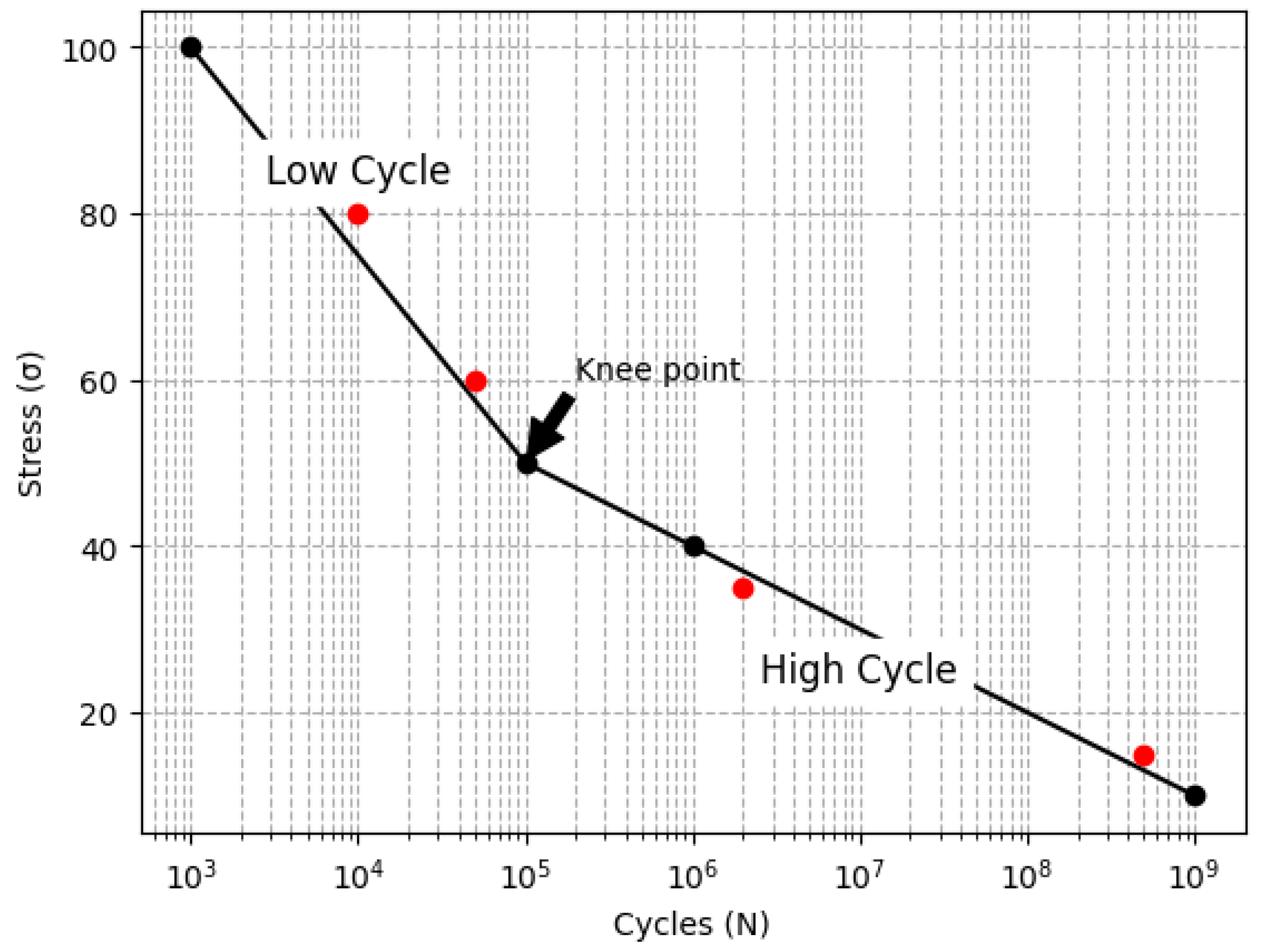
The bilinear model extends the analysis of the linear model used in fatigue analysis. In bilinear behavior, the S–N curve of a material is divided into two regions because of slope changes. For example, Region I can be governed by the plastic region, while Region II can be governed by the elastic zone. The point where the two regions intersect is called the knee-point [4]. The S–N curve, shown in Figure 1, is characterized by a high slope in the first phase of the bilinear model, and a low slope in the second phase.

Understanding the characteristics of the S–N curve, particularly the knee-point, is crucial for fatigue analysis. The high slope in the first phase indicates a higher rate of damage accumulation, whereas the second phase, with its lower slope, suggests a slower progression of fatigue. Moreover, because fatigue is random, then a probability function is necessary, to consider the spread of fatigue data. Thus, here, we use the Weibull distribution. Its generalities are as follows.

2.3. Weibull Distribution

The Weibull distribution is widely used in reliability analysis [14]. It was proposed by Wallody Weibull [15], and its probability density function (pdf) is given by:

$$f\left(t\right)={\displaystyle \frac{\beta }{\eta }}{\left({\displaystyle \frac{t}{\eta }}\right)}^{\beta -1}\exp \left\{-{\left({\displaystyle \frac{t}{\eta }}\right)}^{\beta }\right\}$$

(2)

The corresponding reliability and cumulative failure distributions are:

$$R\left(t\right)=\exp \left\{-{\left({\displaystyle \frac{t}{\eta }}\right)}^{\beta }\right\}$$

(3)

$$F\left(t\right)=1-\exp \left\{-{\left({\displaystyle \frac{t}{\eta }}\right)}^{\beta }\right\}$$

(4)

where $\beta$ is the shape parameter and $\eta$ is the scale parameter. Furthermore, the Inverse Power Law (IPL) model, which is frequently used to relate failure times with non-thermal stresses [16], is defined by:

$$L\left(S\right)={\displaystyle \frac{1}{K{S}^n}}$$

(5)

where $L$ represents the characteristic life, $S$ represents the stress level, and $K$ and $n$ are parameters to be determined. By setting $\eta =L\left(S\right)$ in Equation (5), the Weibull/IPL model is as follows:

$$f\left(t,S\right)=\beta K{S}^n{\left(K{S}^{n}t\right)}^{\beta -1}{e}^{-{\left(K{S}^{n}t\right)}^{\beta }}$$

(6)

Thus, the Weibull/IPL reliability function is given by:

$$R\left(T,S\right)=e^{-{\left(K{S}^{n}T\right)}^{\beta }}$$

(7)

The parameters ($\beta$, $K$, and $n$) of the Weibull/IPL model defined in Equation (6) are estimated by using the maximum likelihood method. With these Weibull/IPL parameters, the steps to perform the P–S–N analysis are as follows.

3. Steps of the Proposed Method

The novelty of the proposed method consists of considering the probabilistic behavior in bilinear fatigue analysis and to generate its corresponding P–S–N field. The material used for the analysis is 42CrMo4 steel. Since the material S–N curve represents median values, then here the analysis is on based on the median stress value of the collected data (see

Table 1. Fatigue test of 42CrMo4 steel.

	${\mathit{s}}_1$								${\mathit{s}}_2$
Cycles (N)	248	260	280	300	750	770	1050	1270	5000	7700	7950	17,200	18,400	27,900	81,000	90,000	152,000	195,000	290,000
Stress (S) MPa	890.4	947.5	934.8	933.7	822.8	790.6	793.1	796.6	679.2	665.3	668.8	649.6	637.3	639.5	595.7	595.7	586.4	553.3	558.7

), and on the Weibull parameters in cycles that are equivalent to this median stress value, $W\left(\beta =4.8031, \eta =1445.7 \mathrm{cycles}\right)$. Consequently, by considering $\beta$ to be constant, the P–S-N percentiles were determined around $\eta =1445.7$ cycles. However, because for each estimated P–S–N percentile, a unique eta (${\eta }_i$) and $R\left(t_i\right)$ value exists, the confidence reliability percentile (CL) value that represents the difference between the ${\eta }_i$ value and ${\eta }_i=1445.7$ cycles was also determined. Additionally, the formulation to relate the $CL$ value with the P–S–N percentile is also given. Therefore, a summary that shows the P–S–N percentile, the $CL$ value, the $R\left(t\right)$ index and the minimum and maximum ${\eta }_i$ values for the one, two, and three sigma levels, as well as those corresponding to the capability $Cp$ and ability $Cpk$ indices is given.

Step 0. Collect experimental fatigue data. Collected data must contain failure times and their corresponding stress value.

Step 1. Separate data into two homogeneous sets $s_1$ and $s_2$. To ensure that the separation is accurate, you can perform the following steps to identify the knee-point, which will help you to confirm that the points in each set are correctly categorized.

Step 1.1. Determine the optimal slopes associated with each set. To achieve this, the failure times must be arranged in ascending order based on the number of cycles to failure. Following this, the optimal slopes ($A_1$ and $A_2$) and intersections ($B_1$ and $B_2$) with the vertical axis for each data set are determined for each value using the least squares method.

$$A_1={\displaystyle \frac{m{\sum }_{i=1}^m\left(\log \left(S_i\right)·\log \left(N_i\right)\right)-{\sum }_{i=1}^m\left(\log \left(S_i\right)\right)·{\sum }_{i=1}^m\left(\log \left(N_i\right)\right)}{m{\sum }_{i=1}^m\left(\log {\left(N_i\right)}^2\right)-{\left({\sum }_{i=1}^m\log \left(N_i\right)\right)}^2}}$$

$$A_2={\displaystyle \frac{\left(n-m\right){\sum }_{i=m+1}^n\left(\log \left(S_i\right)·\log \left(N_i\right)\right)-{\sum }_{i=m+1}^n\left(\log \left(S_i\right)\right)·{\sum }_{i=m+1}^n\left(\log \left(N_i\right)\right)}{\left(n-m\right){\sum }_{i=m+1}^n\left(\log {\left(N_i\right)}^2\right)-{\left({\sum }_{i=m+1}^n\log \left(N_i\right)\right)}^2}}$$

$$B_1={\displaystyle \frac{{\sum }_{i=1}^m\log \left(S_i\right)-A_1{\sum }_{i=1}^m\log \left(N_i\right)}{m}}$$

$$B_2={\displaystyle \frac{{\sum }_{i=m+1}^n\log \left(S_i\right)-A_2{\sum }_{i=m+1}^n\log \left(N_i\right)}{n-m}}$$

where $m$ is the total number of elements of $s_1$ and $n$ is the total number of elements performed.

Step 1.2. Determine the knee-point. Using the values obtained in Step 1.1, identify the point where the slope changes by applying the equations:

$$\log \left(N_{knee}\right)=-{\displaystyle \frac{B_1-B_2}{A_1-A_2}}$$

$$S_{knee}=A_1·\log \left(N_{knee}\right)+B_1$$

where $N_{knee}$ is in cycles and $S_{knee}$ is in stress. The elements above the knee-point belong to $s_1$, while those below are assigned to $s_2$.

Step 2. Determine the data set that provides the best fit between time and stress: For each set, determine the multiple regression coefficient $R^2$, and select the data set with the highest $R^2$ value as the basis for performing the P–S–N analysis.

Step 3. For each data set, determine the Weibull/IPL parameters (${\beta }_i$, $K_i$, and $n_i$) defined in Equation (6).

Step 4. For both sets, determine the reliability $R\left(t\right)$ index corresponding to each observed failure time using Equation (7).

Step 5. Determine the ${\eta }_i$ values corresponding to each stress value in sets $s_1$ and $s_2$, using the respective ${\beta }_i$, $K_i$, and $n_i$ parameters obtained from the set selected for the P–S–N analysis in Equation (5).

Step 6. Using the ${\beta }_2$, $K_2$, and $n_2$ parameters of $s_2$, determine the equivalent failure times of set one (say $s_1$) that corresponds to the same reliability percentile ($R\left(s_1\right)=R\left(s_2\right)$) in set two (say $s_2$). They are given by:

$$N_{eq}={\left(-\ln \left(R\left(t_i\right)\right)\right)}^{{\displaystyle \raisebox{1ex}{$1$}\!\left/ \!\raisebox{-1ex}{$\beta $}\right.}}·{\eta }_i$$

(8)

Step 7. Form the whole data set for the analysis of the P–S–N field by adding to set $s_2$ the equivalent failure times determined in step 6 ($s_2$ is the set with the highest $R^2$ index).

Step 8. Determine the median stress from the experimental stress data.

Step 9. Determine the $\eta$ value in cycles that correspond to the median stress by using the median stress value in Equation (5) with the Weibull/IPL parameters of set $s_2$.

Step 10. Based on the reliability indices calculated in step 5, and the $\eta$ value in cycles of step 9 in Equation (8), determine the predicted failure times. Then, using the maximum likelihood method, determine the Weibull parameters and the corresponding Fisher matrix. And by using the Fisher matrix data in Equation (9), determine the standard deviation of the eta $\eta$ parameter as:

$${\sigma }_{\eta }=\sqrt{Var\left(\eta \right)}$$

(9)

Step 11. Use Equations (10) and (11) to determine the upper and lower limits of $\eta$ corresponding to a desired $k_{\alpha }$ percentile.

$${\eta }_U=\eta ·{\exp }^{{\displaystyle \frac{k_{\alpha }\sqrt{var\left(\eta \right)}}{\eta }}} \left(\mathrm{upper} \mathrm{bound}\right)$$

(10)

$${\eta }_L={\displaystyle \frac{\eta }{{\exp }^{\frac{k_{\alpha }\sqrt{var\left(\eta \right)}}{\eta }}}} \left(\mathrm{lower} \mathrm{bound}\right)$$

(11)

where $k_{\alpha }$ is the $z$ value of the normal distribution that corresponds to the desired two sizes percentile determined as:

$$\alpha ={\displaystyle \frac{1-\delta }{2}}$$

(12)

which for one-sided bound is expressed as:

$$\alpha =1-\delta$$

(13)

where $\mathsf{\delta }$ is the corresponding confidence level. The numerical application is as follows.

4. Case Study

This section presents the steps to determine the P–S–N field of fatigue data with bilinear behavior, its corresponding Weibull family, and testing plan. The bilinear analysis is as follows.

4.1. Bilinear Numerical Analysis

The application is performed using the 42CrMo4 steel material. Its mechanical properties are Modulus of elasticity of 210 GPa, Poisson ratio of $0.30$, and shear modulus of 80 GPa. The numerical application aims to demonstrate how the methodology enables the determination of the P–S–N field of 42CrMo4 steel. The methodological steps to perform the bilinear analysis are as follows.

Step 0: Collected the experimental data with bilinear behavior. The collected data are represented graphically in Figure 2, where the knee-point separates the elements into two data sets, and the failure times of both sets are provided in Table 1.

Step 1. Based on the knee-point, the addressed two bilinear behavior groups are $s_1$ and $s_2$. Data were published in [17].

Step 2. Because the $R^2$ index for $s_1$ data is 0.8083, and for $s_2$ data is 0.8280, we select the $s_2$ set as the base set for performing the P–S–N analysis.

Step 3. By applying the maximum likelihood method to the Weibull/IPL model defined in Equation (6), the estimated parameters for each data set are and its corresponding $LK$ value given in

Table 2. Weibull/IPL parameters for data sets.

	$\mathit{\beta }$	$\mathit{K}$	$\mathit{n}$	LK
$s_1$	6.2428	4.74 × 10−28	8.3738	−48.132
$s_2$	4.8031	3.43 × 10−61	20.0032	−115.5793

.

Step 4. Using Equation (7) and the parameters from Table 2, the reliability indices of the failure times of both data sets are given in

Table 3. Reliability of failure times of ${\mathit{s}}_1$ and ${\mathit{s}}_2$.

	${\mathit{s}}_1$								${\mathit{s}}_2$
Cycles (N)	248	260	280	300	750	770	1050	1270	5000	7700	7950	17,200	18,400	27,900	81,000	90,000	152,000	195,000	290,000
R(t)	0.9643	0.2838	0.3724	0.2396	0.5560	0.9177	0.4957	0.0552	0.7606	0.7419	0.5620	0.2396	0.7299	0.0393	0.5527	0.3740	0.0680	0.9671	0.5640

.

Step 5. By using the ($\beta$, $K$, and $n$) parameters of the set with the highest $R^2$ (in this case, the parameters of $s_2)$ in Equation (5), the ${\eta }_i$ values corresponding to each stress value of $s_1$ and $s_2$ are given in

Table 4. Weibull scale parameter for ${\mathit{s}}_1$ and ${\mathit{s}}_2$ using Weibull/IPL parameters of $s_2$.

	${\mathit{s}}_1$								${\mathit{s}}_2$
${\eta }_i$	29.1	8.4	11	11.2	141.2	313.8	294.6	269.8	6548.7	9903.5	8916.7	15,968.1	23,405.7	21,846.6	90,311.3	90,311.3	123,719.2	395,533.9	325,694.3
Stress (S) MPa	890.4	947.5	934.8	933.7	822.8	790.6	793.1	796.6	679.2	665.3	668.8	649.6	637.3	639.5	595.7	595.7	586.4	553.3	558.7

.

Step 6. Based on the $R\left(t\right)$ index of Table 3 and the Weibull scale values of Table 4, from Equation (8) the equivalent failure times $N_{eq}$ of data set $s_1$, that should be incorporated to the $s_2$ set data, are given in

Table 5. Equivalent failure times of ${\mathit{s}}_1$ that should be incorporating into ${\mathit{S}}_2$.

	${\mathit{s}}_1$
R(t)	0.9643	0.2838	0.3724	0.2396	0.5560	0.9177	0.4957	0.0552
Neq	14.6	8.8	10.9	12.1	126.4	188.2	273.7	336.7

.

Step 7. The complete data set, which includes the equivalent failure times from Table 5 into data of set $s_2$ is given in

Table 6. Grouped ${\mathit{s}}_1$ and ${\mathit{s}}_2$ data set.

	${\mathit{s}}_1$								${\mathit{s}}_2$
Ngrouped	14.6	8.8	10.9	12.1	126.4	188.2	273.7	336.7	5000	7700	7950	17,200	18,400	27,900	81,000	90,000	152,000	195,000	290,000
Stress (S)	890.4	947.5	934.8	933.7	822.8	790.6	793.1	796.6	679.2	665.3	668.8	649.6	637.3	639.5	595.7	595.7	586.4	553.3	558.7

.

Step 8. Based on the Weibull family of the complete set of stress values from Table 6 (represented as $W \left(\beta =5.9148, \eta =779.3\right)$), the median stress value is $S=732.4$ MPa.

Step 9. From the IPL function defined in Equation (5), the $\eta$ value in cycles corresponding to the median stress value from step 8 is $\eta =1445.7$ cycles.

Step 10. Using the reliability indices of $s_1$ and $s_2$ from Table 3 and using the $\eta$ value from step 9 as a constant in Equation (3), the predicted failure times are given in

Table 7. Predicted failure times for ${\mathit{s}}_1$ and ${\mathit{s}}_2$.

	${\mathit{s}}_1$								${\mathit{s}}_2$
Npre	725.2	1516.8	1442.0	1557.2	1293.9	867.1	1342.9	1804.1	1103.8	1124.0	1288.9	1557.2	1136.5	1846.3	1296.6	1440.7	1776.1	712.7	1287.2
R(t)	0.9643	0.2838	0.3724	0.2396	0.5560	0.9177	0.4957	0.0552	0.7606	0.7419	0.5620	0.2396	0.7299	0.0393	0.5527	0.3740	0.0680	0.9671	0.5640

.

By using the maximum likelihood method and the predicted data in Equation (2), the estimated Weibull parameters are $\beta =4.8031$, $\eta =1445.7$ cycles, with Fisher matrix given as:

$$\left(\begin{array}{cc}0.7690& 19.8171\\ 19.8171& 5278.8121\end{array}\right)$$

From the Fisher matrix, the standard deviation of $\eta$ is ${\sigma }_{\eta }=\sqrt{5278.8121}=72.6$ cycles.

Step 11. Using $\eta =1445.7$ cycles in Equations (10) and (11), the upper and lower limits of the P–S–N field are given in

Table 8. Upper and lower limits of η for several failure percentiles.

Percentile	50%	55%	1σ	80%	90%	95%	2σ	97%	99%	3σ
ηL	1445.7	1437.8	1411.6	1393.9	1367.6	1346.2	1327.9	1315.3	1307.0	1257.0
ηU	1445.7	1453.6	1480.6	1499.4	1528.3	1552.5	1573.8	1589.0	1599.1	1662.6

.

The percentiles in Table 8 represent the P–S–N field around the $\eta$ value ($1445.7$ cycles) corresponding to the analyzed median stress ($732.4$ MPa). Here, we use the median stress because the S–N curve represents median values, but any other desired stress value can be used. Therefore, the Weibull distribution that represents the median stress of the bilinear behavior in cycles is $W\left(4.8031, 1445.7 \mathrm{cycles}\right)$, and its P–S–N field are given in Table 8. Now, the testing plan to determine the reliability index represented by the addressed Weibull distribution is as follows.

4.2. Test Plan of the Addressed Weibull Distribution

Here, we numerically perform the vibration test plan given in Appendix C of the GMW3172 users guide. The steps to perform this test plan for the addressed bilinear Weibull distribution are as follows.

Step 1. Determine the six test plan elements. They are: (1) Required reliability $R\left(t\right)$. (2) Required confidence level $CL$ for the desired $R\left(t\right)$ index. (3) The sample size $n$ to be tested. (4) The testing time $t$. (5) The Weibull ($\beta$ and $\eta$) parameters. And (6) The testing conditions.

Step 2. Determine the required sample size $n$ corresponding to the addressed $\eta$ value. Based on Piña-Monarrez [18], it is given by:

$$n={\displaystyle \frac{-1}{\ln \left(R\left(t\right)\right)}}$$

(14)

Step 3. Determine the required testing time. It is the time that corresponds to the desired reliability $R\left(t\right)$ index. From [19], and using the $n$ value of Equation (14) and the bilinear Weibull parameters of step 1, it is given by:

$$t={\displaystyle \frac{\eta }{n^{1/\beta }}}$$

(15)

Step 4. Determine the $n_2$ value that corresponds to the required $R\left(t\right)$ and $CL$ indices from step 1 as:

$$n_2={\displaystyle \frac{\ln \left(1-CL\right)}{\ln \left(R\left(t\right)\right)}}$$

(16)

Step 5. Using the $n_2$ value, determine the corresponding upper Weibull eta ${\eta }_U$ parameter as:

$${\eta }_U=n_2^{{\displaystyle \raisebox{1ex}{$1$}\!\left/ \!\raisebox{-1ex}{$\beta $}\right.}}t$$

(17)

Step 6. From Piña-Monarrez [18], determine the lower ${\eta }_L$ parameter as:

$${\eta }_L={\displaystyle \frac{{\eta }^2}{{\eta }_U}}$$

(18)

Step 7. Using the testing time $t$ from step 3 and ${\eta }_U$ from step 5 in Equation (3), determine the corresponding reliability index.

Step 8. Determine the P–S–N percentile corresponding to the required $CL$ value from step 1 as:

$$k_{\alpha }=-\ln \left({\left({\displaystyle \frac{{\eta }_L}{{\eta }_U}}\right)}^{{\displaystyle \raisebox{1ex}{$1$}\!\left/ \!\raisebox{-1ex}{$2$}\right.}}\right)\ast \left({\displaystyle \frac{\eta }{{\sigma }_{\eta }}}\right)$$

(19)

where ${\sigma }_{\eta }$ was determined in Step 10 of Section 4.1, using data from the Fisher matrix in Equation (9). The numerical application is presented as follows.

4.3. Numerical Application of the Test Plan

Steps 1, 2, and 3. The test plan includes six essential elements, including the required reliability index $R\left(t\right)=0.97$ and confidence level $CL=0.75$, as specified by the GMW3172 standard. The Weibull family derived in Section 4.1, are $\beta =4.8031$ and $\eta =1445.7$ cycles. The sample size associated with $\eta$, calculated using Equation (14) is $n=32.8$, while the required testing time, determined using Equation (15) is $t=698.8$ cycles.

Step 4. Using Equation (16), the required sample size $n_2$ corresponding to $R\left(t\right)$=0.97 and $CL=0.75$ is $n_2=$ 45.5.

Step 5. By substituting $n_2=$ 45.5 into Equation (17), the upper bound of the Weibull scale parameter is ${\eta }_U=1547.4$ cycles.

Step 6. Using Equation (18), the lower bound of the Weibull scale parameter is determined as ${\eta }_L=1350.6$ cycles.

Step 7. Using the test time calculated in step 3, the reliability index corresponding to ${\eta }_U=1547.4$ cycles is determined as $R\left(t\right)=0.9783$. Note that, because no failures are allowed in this testing plan, the $R\left(t\right)$ index for the lower value was not determined.

Step 8. For the selected sigma levels (one sigma, two sigma, and three sigma) and Cp and Cpk indices, using the standard deviation ${\sigma }_{\eta }=72.6$ cycles in Equations (17) and (18) the corresponding normal percentiles, Weibull upper (${\eta }_U)$ and lower (${\eta }_L)$ scale parameter limits, confidence level ($CL$), and reliability $R\left(t\right)$ indices were determined. The results are presented in

Table 9. Normal and Weibull data with their corresponding $R\left(t\right)$ indices.

	Normal Percentiles	${\mathit{k}}_{\mathit{\alpha }}$	ηU	ηL	CL	R(t)
1σ	0.6827	0.4752623	1480.6	1411.5	0.6742	0.9732
Cpk	0.9082	1.3297520	1545.6	1352.2	0.7480	0.9781
Cp	0.9525	1.6695926	1572.2	1329.3	0.7761	0.9798
2σ	0.9545	1.6901461	1573.8	1327.9	0.7777	0.9799
3σ	0.9973	2.7821505	1662.6	1257.0	0.8588	0.9846
Test plan	0.0880	−1.3531742	1547.4	1350.6	0.7500	0.9783

. Additionally, Table 9 includes the corresponding data for the designed test plan.

From the last row of Table 9, we observe that by performing the designed test plan, with require $R\left(t\right)=0.97$ and $CL=0.75$, 46 pieces must be tested for a testing time of $t=698.8$ cycles each. If none of them fail, the analyzed element achieves a minimum reliability of $R\left(t\right)=0.9783$. Note that this occurs because ${\eta }_U$ is greater than $\eta$ ($1547.4>1545.7$). The general conclusions are as follows.

5. Conclusions

1. Although in practice, bilinear behavior is mainly attributed to the interaction of two competitive failure modes, this paper focuses on the bilinear behavior of the S–N curve for the 43CrMo4 steel material. The proposed methodology, however, can be applied to analyze any type of bilinear behavior.

2. By applying the proposed methodology, the Weibull distribution modeling the linear behavior is identified and used to design the test plan to validate the required reliability index. For this analysis, the median stress is used but any value of stress can be used.

3. The application of the methodology allows us, for any desired percentile of the normal distribution, to determine the elements corresponding to the upper and lower limits of the Weibull scale parameter, their equivalent confidence level, and their reliability index.

4. The developed test plan highlights the importance of reliability and confidence level in determining the required sample size.

5. The proposed methodology enables the determination of the confidence level ($CL$) corresponding to any desired percentile, and vice versa.

6. It is very important to note that the normal and Weibull percentiles depend on the Weibull $\beta$ value. Therefore, an accurate estimation of $\beta$ is critical in the analysis. Therefore, once it is determined, the estimation of the predicted failure times will be efficient.

7. As part of future research, it is recommended to explore the sensitivity of the addressed Weibull family to more accurately determine the expected behavior of $\beta$ and the variance of $\eta$.