TA-RRT*: Adaptive Sampling-Based Path Planning Using Terrain Analysis

Abstract

This paper proposes a novel algorithm, Terrain Analysis–Rapidly exploring Random Tree* (TA-RRT*), which improves the performance of path planning using adaptive sampling and step size based on terrain analysis. While existing RRT*-based algorithms perform node sampling and tree expansion in various ways to optimize path planning, they may still generate inefficient paths in complex terrain environments. In this paper, TA-RRT* analyzes the complexity of the terrain to generate a probability density function, which is then used to guide adaptive sampling and tree expansion during the path planning process. In addition, we reduce the length of generated paths using an adaptive step size based on terrain complexity. To verify the performance of the proposed algorithm, we conduct experiments with various path planning algorithms in three different environments: simple, intermediate, and complex. The experimental results demonstrate that TA-RRT* outperforms other algorithms in terms of path length, computational time, and memory usage. Furthermore, its robustness was validated in dynamic environments, where it effectively performed real-time path replanning to adapt to environmental changes, such as the appearance of new obstacles.

1. Introduction

The development of unmanned vehicle technologies, from drones to autonomous vehicles and robots, has rapidly expanded into both civilian and military applications [1,2,3,4,5,6]. To enhance the autonomy of these vehicles in various environments, extensive research has focused on situational awareness and planning. However, significant technical challenges remain, such as navigating complex terrains, predicting dynamic obstacles, and adapting to environmental changes in real-world scenarios [7,8]. Addressing these challenges requires transforming 2D perception data from sensors like cameras, LiDAR, and radar into practical 2D Bird’s Eye View (BEV) images. This transformation is crucial for enabling path planning and control algorithms that help unmanned vehicles navigate complex environments [9]. This study focuses on path planning for unmanned vehicles, aiming to generate routes that avoid obstacles and efficiently reach their destinations based on maps created through BEV images.

Path planning algorithms have been extensively researched and can be broadly categorized into graph search and sampling approaches [10,11,12]. Graph search-based path planning relies on a pre-constructed graph using previously acquired environmental information, enabling relatively fast shortest-path searches. However, in many unmanned vehicle operations, obtaining and constructing such information in advance is often challenging. Consequently, significant research has focused on methods that explore paths to the target point through random sampling.

Rapidly exploring Random Tree (RRT) [13] and Probabilistic RoadMap (PRM) [14] are representative sampling-based path planning algorithms. RRT explores paths by expanding a tree structure through random sampling, and can find a path to the target point with a high probability when a sufficient number of nodes are sampled. However, it does not guarantee optimality. The path optimality is primarily defined in terms of cost, which generally includes factors such as path length, energy consumption, and so on. RRT* improves upon RRT by restructuring the tree during node expansion, thereby enhancing the optimality of the explored path [15].

Since the introduction of RRT*, various modified algorithms have been developed to further enhance path optimality [16,17,18,19]. Although RRT* can find a path that connects the starting point to the goal, the generated path is not always the shortest. To address these limitations, algorithms such as Informed-RRT* and RRT*-Smart have been proposed [17,18]. Informed-RRT* generates an initial path, then defines an ellipse using the start and goal points, along with the path length, as parameters [17]. Additional nodes are sampled within this ellipse to improve the initial path, with the ellipse being iteratively reconfigured to further enhance path efficiency. RRT*-Smart also generates an initial path and improves it by designating key points in the environment, such as terrain corners, as beacons [18]. Additional nodes are sampled near these beacons to update and improve the path. Although these algorithms propose additional sampling regions based on environmental analysis, their ability to improve paths is evident under certain conditions, but may be limited in complex terrains.

Therefore, in this paper, we propose a terrain analysis (TA)-RRT* algorithm which enables effective path planning through terrain analysis. The key features of the proposed algorithm are as follows: First, a probability density function (PDF) is generated based on terrain analysis, and adaptive sampling is applied using this PDF to expand the tree. This approach allows for more effective path reconfiguration. Next, the step size is adaptively adjusted according to the complexity of the terrain. In more complex terrains, a shorter step size is used, which enables more linear connections between nodes and improves the optimality of the generated path.

This paper is structured as follows: Section 2 analyzes existing RRT*-based path planning algorithms. Section 3 describes the proposed TA-RRT* algorithm. Then, Section 4 evaluates the performance of the proposed TA-RRT* with existing RRT*-based algorithms. In Section 5, we discuss various practical considerations, including real-world scenarios and the kinematic model. Finally, Section 6 presents the conclusions of this paper and discusses future research directions.

2. Related Works

2.1. Motivation

The RRT algorithm generates random sample points to expand a tree and explores paths that allow a vehicle to reach its target point [13]. While it has the advantage of quickly exploring complex high-dimensional spaces, it does not guarantee the optimality of the generated path. RRT is a fundamental algorithm that has served as the basis for many studies and improvements in the efficiency of path exploration.

The RRT* algorithm was designed to improve the optimality of paths while maintaining the exploration efficiency of RRT [15]. RRT* reduces the path length by reorganizing the existing tree structure each time a new node is added during the exploration process. However, this restructuring process incurs additional computational costs. RRT* consists of the following key steps:

• Random Sampling: randomly generates sample points to expand the exploration space.
• Node Expansion: finds the nearest node to the sample point and generates a new node in that direction.
• Collision Check: verifies that the path between the new node and the existing nodes does not collide with any obstacles.
• Rewiring: after adding a new node, the connections with surrounding nodes are restructured to improve the optimality of the path.

The pseudocode of RRT* is shown in Algorithm 1.

Algorithm 1 RRT*($q_{init}$, V, E)

1: $V\leftarrow q_{\mathrm{init}}$, $E\leftarrow \varnothing$ 2: for $k=1$ to K do 3:       $q_{\mathrm{rand}}\leftarrow \mathrm{RandomSample}\left(\right)$ 4:       $q_{\mathrm{nearest}}\leftarrow \mathrm{Nearest}(T,q_{\mathrm{rand}})$ 5:       $q_{\mathrm{new}}\leftarrow \mathrm{Steer}(q_{\mathrm{nearest}},q_{\mathrm{rand}})$ 6:       if $\mathrm{CollisionCheck}(q_{\mathrm{nearest}},q_{\mathrm{new}})$ then 7:             $V\leftarrow V\cup \left\{q_{\mathrm{new}}\right\}$ 8:             $Q_{\mathrm{near}}\leftarrow \mathrm{Near}(T,q_{\mathrm{new}},r)$ 9:             $\mathrm{ChooseParent}(Q_{\mathrm{near}},q_{\mathrm{nearest}},q_{\mathrm{new}},E)$ 10:           $\mathrm{Rewiring}(Q_{\mathrm{near}},q_{\mathrm{new}},E)$ 11:     end if 12: end for

Here, V represents the set of nodes, which initially contains only the starting point $q_{\mathrm{init}}$. E represents the set of edges, which is initially empty. K denotes the maximum number of iterations of the algorithm. $q_{\mathrm{rand}}$ is a randomly generated sample point, $q_{\mathrm{nearest}}$ is the node in the tree T closest to $q_{\mathrm{rand}}$, $q_{\mathrm{new}}$ is the new node expanded from $q_{\mathrm{nearest}}$ in the direction of $q_{\mathrm{rand}}$, $Q_{\mathrm{near}}$ is the set of nodes near $q_{\mathrm{new}}$, and r is the radius used to search for nearby nodes.

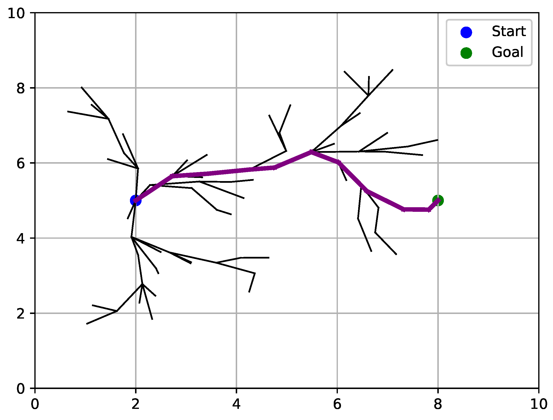
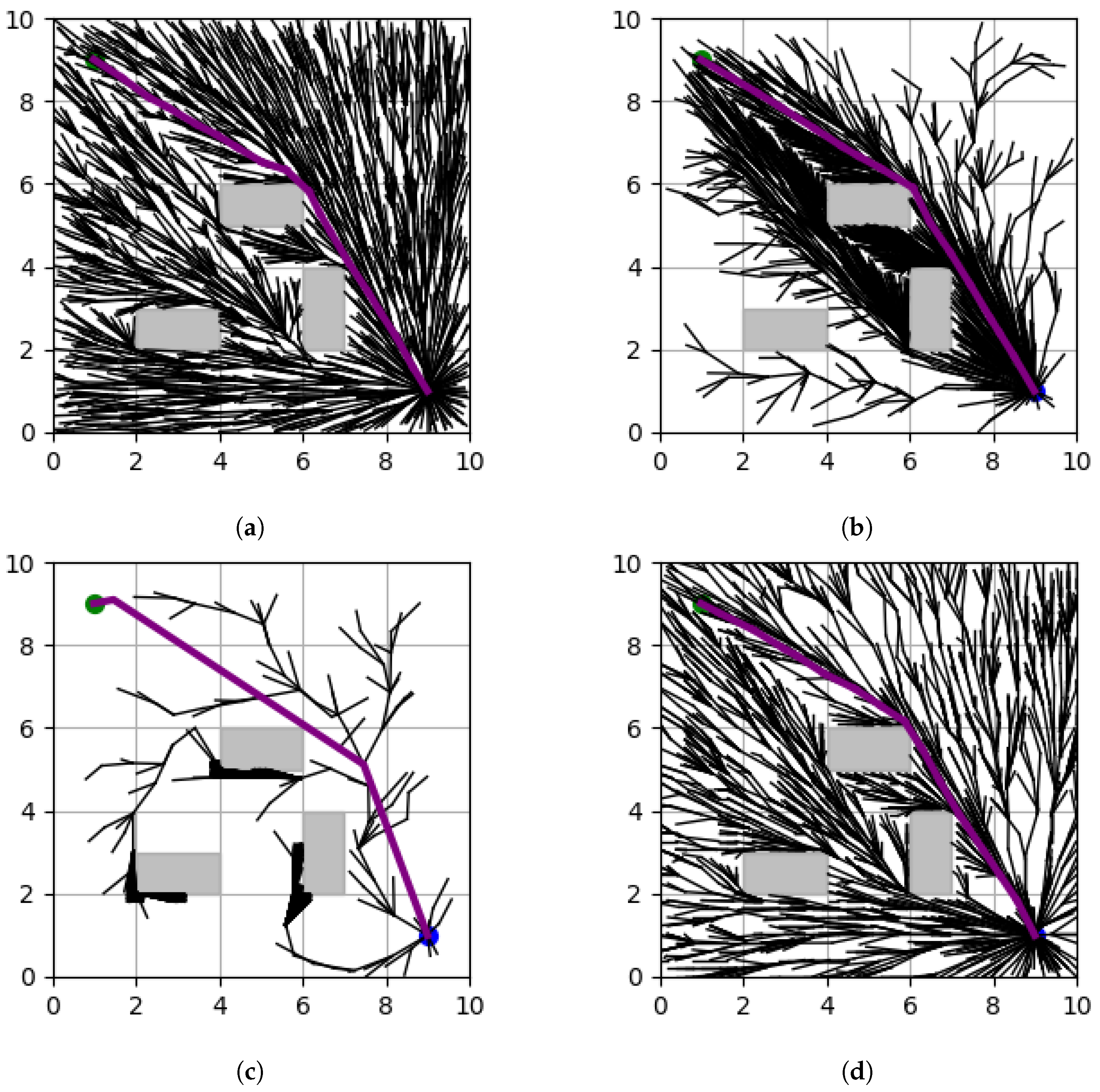
The RRT* algorithm can find a path that connects the starting point to the goal by expanding the tree. However, as shown in Figure 1, the resulting path (purple line) may not be the shortest path between the two points.

To overcome these limitations and derive more efficient paths, algorithms such as Informed-RRT* and RRT*-Smart have been proposed [17,18]. These algorithms build upon RRT* by enhancing path efficiency through node sampling in a limited region after generating the initial path. Informed-RRT* first generates an initial path, then defines an ellipse using the start and goal points, along with the path length, as parameters [17]. Additional nodes are sampled within this ellipse to improve the initial path, with the ellipse being reconfigured iteratively to further enhance path efficiency. RRT*-Smart also generates an initial path, then improves it by designating key points in the environment, such as terrain corners, as beacons [18]. Additional nodes are sampled near these beacons to update and improve the path.

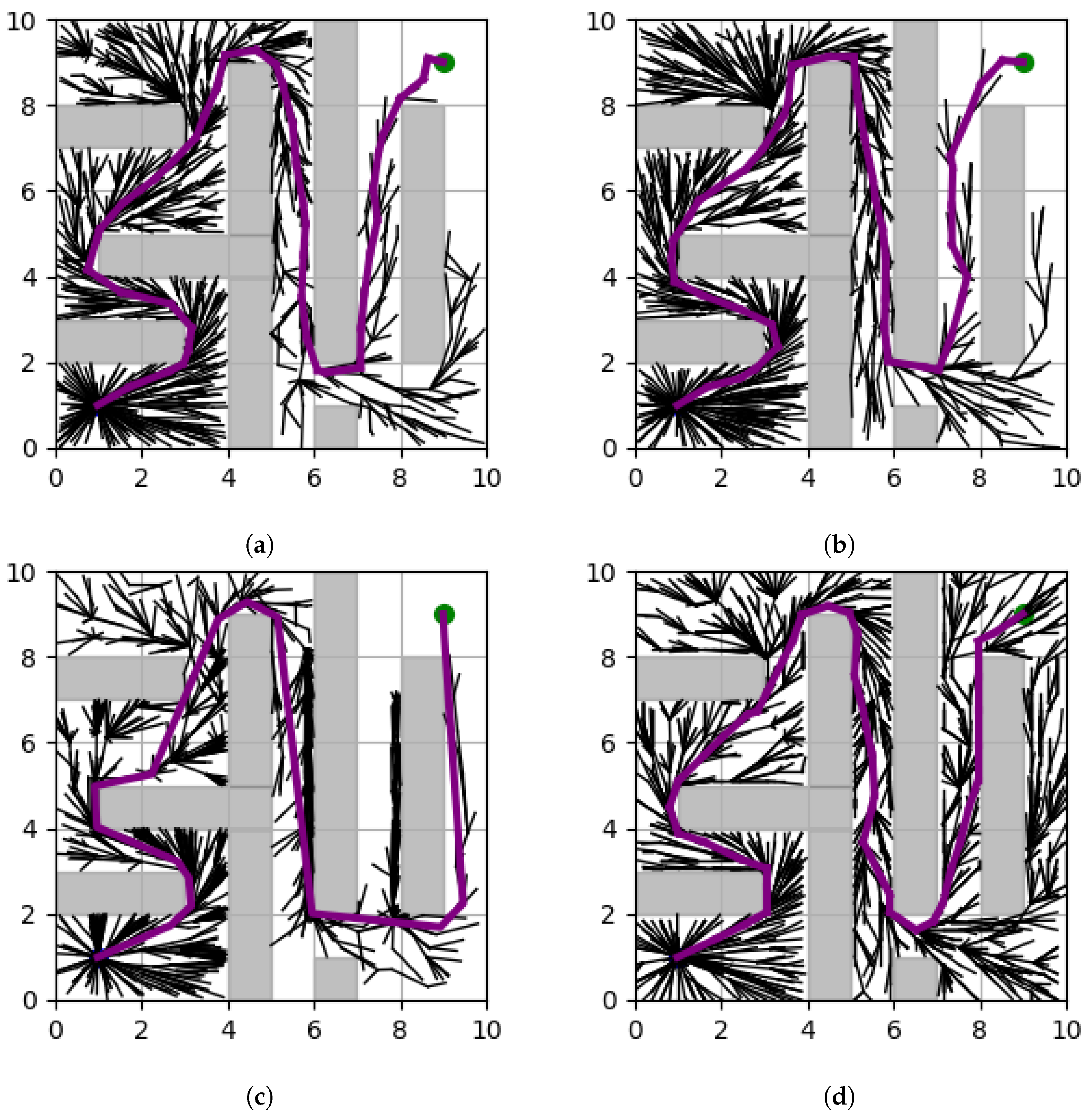
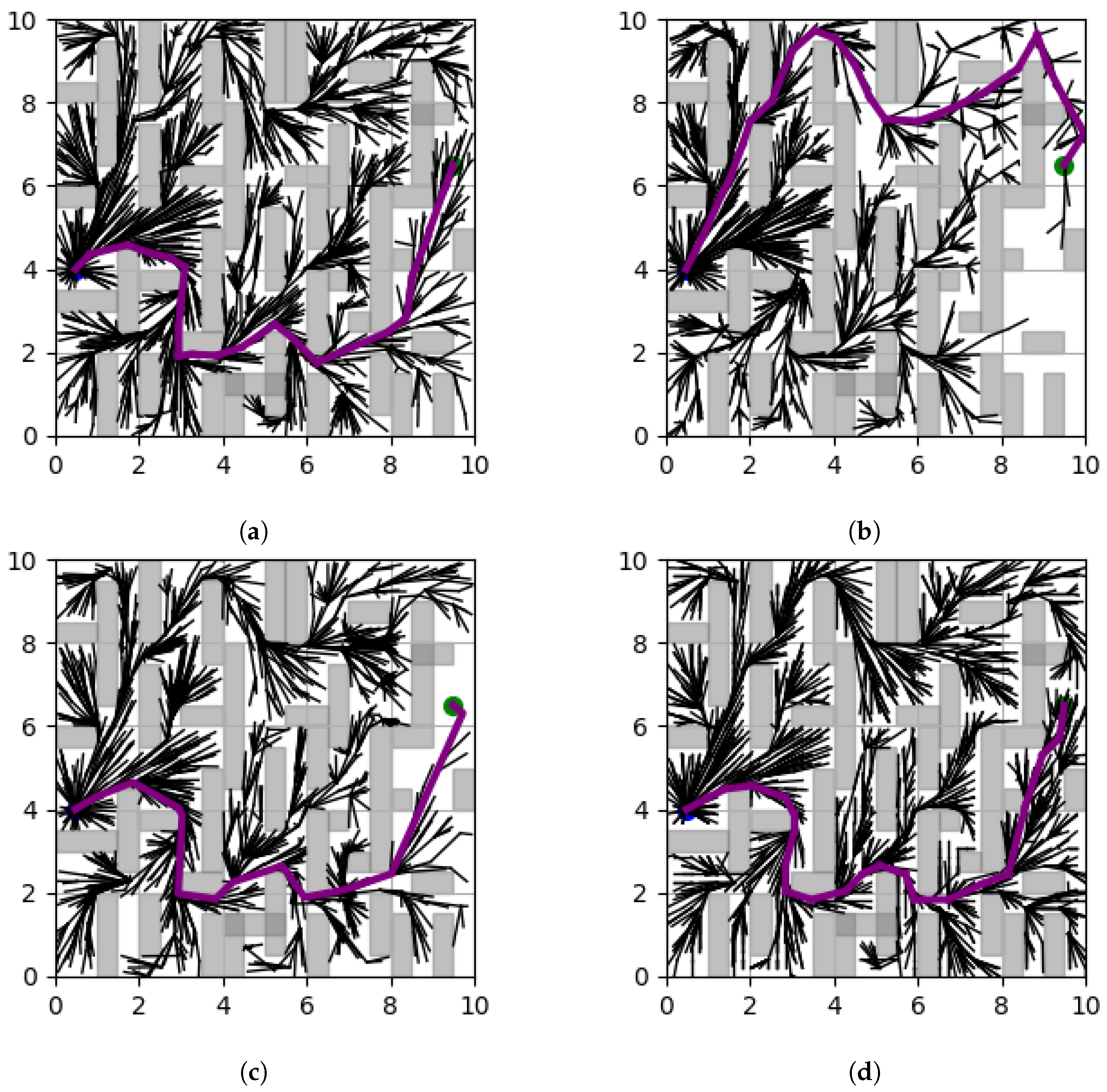
These algorithms propose additional node sampling regions based on an intuitive analysis of the environment. As a result, they can improve paths in certain conditions, but their effectiveness is limited in other scenarios, particularly in complex terrains. Therefore, this paper proposes the TA-RRT* algorithm, which is based on terrain analysis and is designed to enable more effective path planning, even in complex terrain environments.

2.2. Comparison with Recent RRT*-Based Path Planning

Recent advancements in RRT*-based algorithms have primarily focused on improving sampling efficiency, path optimality, and adaptability to diverse environments. Notable examples include Gaussian Mixture Regression-based RRT* (GMR-RRT*) [1] and deep learning-enhanced RRT*, which leverage probabilistic models and neural networks to guide sampling toward optimal regions [20]. While these methods demonstrate significant performance improvements in structured environments, their reliance on extensive computational resources and pre-trained models often limits their applicability in real-time scenarios.

In contrast, the proposed TA-RRT* algorithm adopts a lightweight and adaptive strategy by integrating terrain-based probability density functions and step size adjustments. Unlike GMR-RRT*, which depends on prior training data, TA-RRT* dynamically analyzes the terrain during execution, enabling efficient real-time sampling without pre-computed models. Similarly, compared to deep learning-based methods, TA-RRT* strikes a balance between computational complexity and path quality, making it particularly suitable for resource-constrained applications such as autonomous robotics.

3. Proposed Method

3.1. TA-RRT* Overview

To overcome the limitations of existing algorithms, we propose an RRT*-based path planning algorithm that incorporates adaptive sampling and a step size based on terrain analysis.

Algorithm 2 presents the pseudocode for the proposed TA-RRT* algorithm. Here, V denotes the set of nodes, which initially contains only the starting point $q_{\mathrm{init}}$. E denotes the set of edges, which starts as being empty. K indicates the maximum number of iterations. $q_{\mathrm{rand}}$ is a randomly generated sample point, $q_{\mathrm{nearest}}$ is the closest node in the tree T to $q_{\mathrm{rand}}$, $q_{\mathrm{new}}$ is the new node expanded from $q_{\mathrm{nearest}}$ towards $q_{\mathrm{rand}}$, $Q_{\mathrm{near}}$ is the set of nodes near $q_{\mathrm{new}}$, and r is the radius used for searching nearby nodes.

Algorithm 2 is similar to RRT*, with the key differences highlighted. The proposed algorithm analyzes the terrain of the operating environment to extract the terrain corners (C) and uses this information to generate a PDF (P) for node sampling (Lines 2–3). Paths that pass near obstacles can be shortened when they approach the vertices of the terrain [18,21]. Based on this principle, a PDF is generated to increase the likelihood of node occurrence near these vertices and along the paths between them. Nodes are sampled to expand the tree. Initially, nodes are sampled based on a uniform distribution. However, once the initial path is created, nodes are sampled according to the PDF (P) generated from the terrain corners (C). To improve path length through random exploration, an $\epsilon$-greedy strategy is applied [22], combining random sampling from a uniform distribution with adaptive sampling based on the PDF at a specified ratio (Lines 5, 7–9). The process of generating the terrain-based PDF and performing adaptive sampling is described in Section 3.2.

Algorithm 2 TA-RRT*($q_{init}$, V, E)

1: $V\leftarrow q_{\mathrm{init}}$, $E\leftarrow \varnothing$ 2: $C\leftarrow \mathrm{TerrainAnalysis}\left(\right)$ 3: $P\leftarrow \mathrm{GeneratePDF}\left(C\right)$ 4: for $k=1$ to K do 5:       if $(\epsilon <{\epsilon }_{th})$ or $(\mathrm{not}\mathrm{InitialPathFound})$ then 6:             $q_{\mathrm{rand}}\leftarrow \mathrm{RandomSample}\left(\right)$ 7:       else 8:             $q_{\mathrm{rand}}\leftarrow \mathrm{RandomSampleFromPDF}\left(P\right)$ 9:       end if 10:     $q_{\mathrm{nearest}}\leftarrow \mathrm{Nearest}(T,q_{\mathrm{rand}})$ 11:     $q_{\mathrm{new}}\leftarrow \mathrm{AdaptiveSteer}(q_{\mathrm{nearest}},q_{\mathrm{rand}},C)$ 12:     if $\mathrm{CollisionCheck}(q_{\mathrm{nearest}},q_{\mathrm{new}})$ then 13:           $V\leftarrow V\cup \left\{q_{\mathrm{new}}\right\}$ 14:           $Q_{\mathrm{near}}\leftarrow \mathrm{Near}(T,q_{\mathrm{new}},r)$ 15:           $\mathrm{ChooseParent}(Q_{\mathrm{near}},q_{\mathrm{nearest}},q_{\mathrm{new}},E)$ 16:           $\mathrm{Rewiring}(Q_{\mathrm{near}},q_{\mathrm{new}},E)$ 17:     end if 18: end for

Subsequently, the step size is adaptively adjusted according to the terrain complexity. In complex terrains, a shorter step size allows for precise path exploration, while in simpler areas, a longer step size facilitates broader exploration within the given iterations, improving the probability of generating an initial path. This adaptive step size approach, which refines the path by utilizing more nodes, is explained in Section 3.3.

3.2. Terrain Analysis and Adaptive Sampling

Because path exploration is influenced by the complexity of the environment, it is necessary to analyze the terrain for sampling-based path planning in order to improve search efficiency and reduce path length. In this paper, terrain corners are used to generate the PDF and to quantify the complexity of the terrain. To detect corners, various methods, such as the Harris corner detector [23], have been introduced and proven effective in image processing. The Harris corner detector is an edge detection algorithm widely used in computer vision for identifying corners in an image. It assesses local variations in intensity to determine regions with strong directional changes, which are characteristic of corners. However, due to differences in the environments and the need for computational efficiency in path planning, we utilize a simplified corner detection method based on the Harris corner detector.

First, the environment is converted into a grid, and corners are detected by comparing the values of each cell with its neighboring cells as the grid is traversed. Figure 2 shows an example of corner detection within a grid. White and gray areas represent free space and terrain (obstacles), respectively. The star marks the point $g(x,y)$ where corner detection is performed, and the red dashed line indicates the search range used to determine whether $g(x,y)$ is a corner. The ‘X’ symbols indicate locations where the values of $g(x,y)$ differ from those in its adjacent areas. Figure 2a–c shows three different cases of corners. In (a) and (c), $g(x,y)$ represents a convex and concave corner, respectively [24], while (b) represents an edge that is not considered a corner. Based on these observations, corners are detected by analyzing the discrepancies between adjacent grid cells.

Here, $g(x,y)$ denotes the grid cell at the coordinates $(x,y)$, where a value of 0 indicates free space and 1 indicates an obstacle. The number of neighboring cells with different values from a grid $g(x,y)$ with a value of 1, denoted as $N_{disp}$, is calculated as follows.

$$N_{disp}(x,y)=\sum _{\begin{array}{c}dy\in \{-1,0,1\},\\ dx\in \{-1,0,1\},\\ (dx,dy)\ne (0,0)\end{array}}\parallel g(x,y)-g(x+dx,y+dy)\parallel$$

(1)

Then, the corner $C(x,y)$ is determined according to the value of $N_{disp}(x,y)$ as follows:

$$C(x,y)=\left\{\begin{array}{cc}\mathrm{True},\hfill & \mathrm{if}(N_{disp}(x,y)>C_{th})\mathrm{or}(C_{th}==1)\hfill \\ \mathrm{False},\hfill & \mathrm{otherwise}\hfill \end{array}\right.$$

(2)

where $C_{th}$ is the threshold for corner detection, which we set to 3 in this paper.

Next, the identified corners are connected with straight lines, and a PDF is derived using these lines. Figure 3a,b shows the corners (red points) identified using the above detection method and the PDF derived from the lines connecting these corners. In Figure 3a, the black region represents the terrain (obstacle), and the red dots indicate the identified corners. In Figure 3b, the white regions represent high probabilities, while the black regions represent low probabilities.

3.3. Terrain-Based Step Size Adaptation

Algorithm 3 presents the pseudocode for the adaptive steer algorithm. Using the corner C, the terrain density $\rho$, which represents the terrain complexity, and the corresponding adaptive step size $\delta$ are calculated. These values are then used in the steer function to determine the direction and distance of the next step in the path planning process. The pseudocode is as follows:

Algorithm 3 AdaptiveSteer($q_{\mathrm{nearest}},q_{\mathrm{rand}},C)$

1: $\rho \leftarrow \mathrm{CalculateTerrainDensity}(q_{\mathrm{nearest}},C)$ 2: $\delta \leftarrow \mathrm{CalculateStepsize}\left(\rho \right)$ 3: $q_{\mathrm{new}}\leftarrow \mathrm{Steer}(q_{\mathrm{nearest}},q_{\mathrm{rand}},\delta )$

3.3.1. Terrain Density

In this study, the terrain complexity is quantified by converting the terrain into a BEV image and subsequently into a grid map, where the number of detected corners indicates the complexity. If obstacles are represented in the BEV, they can be identified, allowing for the generation of paths that avoid them. First, the terrain corners C around $q_{\mathrm{nearest}}$ are identified to calculate the terrain density $\rho$. Here, $\rho$ is defined as the number of terrain corners, serving as a measure of terrain complexity. A higher $\rho$ indicates a more complex terrain with many corners, while a lower $\rho$ indicates a simpler terrain. A k-dimensional (KD) tree is utilized to calculate $\rho$ efficiently. This data structure partitions the space recursively at each level of the tree, alternating dimensions for division [25]. By using a KD tree, the number of terrain corners within a given radius can be quickly determined by narrowing the search range.

Figure 4a shows an example of the searching result for corners within a radius around a reference point using a KD tree. The gray area represents the terrain (obstacle), and the red dots represent the corners. The KD tree recursively partitions the space, with black and blue dashed lines representing horizontal and vertical divisions. The purple dot and dashed circle represent the reference point and its radius, while the green dots indicate corners within that radius. First, since the variance of the detected corners along the X-axis is greater than that along the Y-axis, the first partition is performed based on the X-axis. At this stage, these nodes are sorted along the X-axis, and the median node (5, 9) is selected as the partitioning point, dividing the space along the X-axis (black dashed line). Next, for the nodes within the left and right subspaces of node (5, 9), these nodes are sorted along the Y-axis, and the median nodes (1, 5) and (8, 2) are chosen to partition the subspaces along the Y-axis (blue dashed lines), respectively. This process continues recursively, alternating between the X-axis and Y-axis at each depth level in the KD tree.

Figure 4b illustrates the tree structure based on these partitions as shown in Figure 4a. The first partition node (5, 9) becomes the root node of the KD tree. Its child nodes are the median nodes of the left and right subspaces, (1, 5) and (8, 2), respectively. This process is recursively applied to each subspace to construct the tree structure. Then, using the constructed tree, the number of corners $\rho$ within the radius R around $q_{\mathrm{nearest}}$ is calculated. For example, as shown in Figure 4a, when the reference point is $q_{\mathrm{nearest}}=(2,6)$ and $R=2$, neither node (5, 9) nor the line dividing the space intersects with the radius. Therefore, as shown in Figure 4b, node (8, 2) and its subordinate nodes are not examined, which allows the KD tree to reduce the computation time for determining terrain density.

3.3.2. Adaptive Step Size

To enhance the efficiency and precision of path planning, we apply an adaptive step size based on terrain density. In more complex terrain, shorter step sizes enable precise path exploration, while longer step sizes are used in simpler terrain to reduce exploration time. A logistic function was used to adjust the step size according to the terrain density, decreasing the step size nonlinearly as density increases. This approach ensures that the step size is appropriately scaled, shorter in complex terrain and longer in simpler terrain, maximizing the efficiency of path exploration. The adaptive step size using the logistic function is as follows:

$$\delta ={\displaystyle \frac{({\beta }_1-{\beta }_2)}{1+exp\{(\rho -{\beta }_3)/\parallel {\beta }_4\parallel \}}}+{\beta }_2.$$

(3)

Here, ${\beta }_1$ and ${\beta }_2$ represent the maximum and minimum step sizes, while ${\beta }_3$ and ${\beta }_4$ correspond to the midpoint (offset) and slope of the logistic function. The values ${\beta }_1=0.7$, ${\beta }_2=0.5$, ${\beta }_3=4$, and ${\beta }_4=0.5$ are empirically used in this paper. Figure 5 illustrates the variation in step size according to terrain density.

4. Experiment

4.1. Experiment Configuration

To validate the performance of TA-RRT*, we conducted experiments to evaluate path planning algorithms. The experiments were carried out in a 10 × 10 square space with randomly placed obstacles. The environment was categorized into three types based on the arrangement of obstacles and the resulting complexity of the paths: simple, intermediate, and complex.

• Simple environment: this environment featured very few obstacles and was primarily used to assess whether the algorithm could plan a path connecting the start and goal points.
• Intermediate environment: this environment contained a moderate number of obstacles and was used to test the algorithm’s ability to plan a path that avoids obstacles.
• Complex environment: this environment included a large number of obstacles and was used to test the algorithm’s ability to plan an appropriate path even in highly complex conditions.

Each experiment was repeated 100 times in each environment to ensure the reliability of the results.

To evaluate the performance of the proposed TA-RRT* algorithm, we conducted comparative experiments against other well-known path planning algorithms. Specifically, we compared TA-RRT* with several widely recognized RRT*-based algorithms, including RRT* [15], Informed-RRT* [17], and RRT*-Smart [18]. The experiments were conducted on a system with an Intel i7-1360P CPU (Intel, Santa Clara, CA, USA), 16 GB RAM, and a software environment set up using Visual Studio Code (version 1.93).

4.2. Experiment in Static Scenarios

4.2.1. Performance Comparison

In this section, we evaluate the performance of each algorithm by analyzing the path planning results across simple, intermediate, and complex environments.

Figure 6 shows the path planning results of the RRT*, Informed-RRT*, RRT*-Smart, and TA-RRT* algorithms in a simple environment. Blue and green dots represent the start and goal points, respectively. Gray areas indicate obstacles, black lines show the expanded trees, and purple lines indicate the final paths. RRT* tends to generate nodes uniformly across the entire map due to its sampling method. Informed-RRT* tends to concentrate new nodes within the ellipse, while the RRT*-Smart focuses nodes around key points, such as the vertices of obstacles. The proposed TA-RRT* tends to concentrate nodes along the straight lines connecting obstacle vertices, guided by $ϵ$-greedy-based sampling, although some nodes are still generated across the map.

Figure 7 and

Table 1. Path planning results in a simple environment.

	Exec. Time (ms)		Path Length		No. of Nodes
	Average	STD	Average	STD	Average	STD
M1	7428.15	255.28	11.72	0.03	2809.54	16.58
M2	12,768.33	757.05	11.68	0.01	2325.18	30.84
M3	11,315.65	4383.81	12.08	0.35	1887.46	195.07
M4	9699.26	973.86	11.71	0.01	2864.34	17.49

Values highlighted in bold represent the best performance.

present the results from 100 repeated experiments in a simple environment. M1 to M4 represent RRT*, Informed-RRT*, RRT*-Smart, and TA-RRT*, respectively. Informed-RRT* demonstrates the shortest average path length, even with a relatively small number of nodes, due to effective sampling within the elliptical region. However, its average execution time is the longest due to node concentration in a narrow area. On the other hand, RRT*-Smart shows a relatively long average path length and high standard deviation, as there are insufficient corners to serve as beacons, making it difficult to effectively sample additional nodes. TA-RRT* demonstrates path planning performance comparable to Informed-RRT*, even in simple environments. In addition, TA-RRT* shows the highest average number of nodes, indicating that it was able to use more nodes to improve the path.

Figure 8 shows the path planning results in the intermediate environment. It is hard to observe a similar tendency for node concentration in a confined area with Informed-RRT* in the intermediate environment, as the elliptical sampling region expands when the path does not follow a straight line. RRT*-Smart aims to produce straighter paths through its optimization process. However, as shown in Figure 8c, the algorithm may struggle to make significant corrections when the environment imposes complex path adjustments, potentially leading to less efficient paths. In contrast, TA-RRT* effectively improves the path through terrain analysis-based sampling, allowing for more consistent and efficient improvements in the path, even in challenging terrains.

Figure 9 and

Table 2. Path planning results in an intermediate environment.

	Exec. Time (ms)		Path Length		No. of Nodes
	Average	STD	Average	STD	Average	STD
M1	4739.59	847.60	29.80	0.63	1450.52	120.25
M2	4347.52	705.95	30.11	0.72	1354.07	112.00
M3	3326.30	362.02	30.01	0.77	1301.64	90.78
M4	8301.36	1034.96	29.27	0.27	2167.50	133.16

Values highlighted in bold represent the best performance.

present the results from 100 repeated experiments in an intermediate environment. Due to the winding path, Informed-RRT* finds it difficult to effectively improve the path through additional sampling within the elliptical region, resulting in a relatively long average path length. TA-RRT* uses terrain analysis-based sampling to effectively improve the path, resulting in the shortest average path length and a small standard deviation, indicating high stability in path planning.

Figure 10 shows the path planning results in a complex environment. As shown in Figure 10d, TA-RRT* utilizes terrain analysis-based sampling to effectively distribute nodes, including areas near the goal point. This approach enables TA-RRT* to maintain robust exploration and identify the shortest paths more efficiently, even in the presence of complex obstacles. In contrast, other algorithms tend to have insufficient sampling near the target point, which can make it challenging to find the optimal path.

Figure 11 and

Table 3. Path planning results in complex environments.

	Exec. Time (ms)		Path Length		No. of Nodes
	Average	STD	Average	STD	Average	STD
M1	12,554.88	1774.46	15.42	0.44	1577.81	146.46
M2	13,709.04	2844.10	15.77	0.66	1526.00	147.89
M3	19,207.87	6002.88	16.04	0.97	1647.15	190.97
M4	23,231.93	2639.77	15.25	0.20	2148.20	127.06

Values highlighted in bold represent the best performance.

show the performance results obtained from 100 repeated experiments in a complex environment. RRT* generally produced short paths, but the high standard deviation in path length indicates low path stability. Due to the simplicity of the path exploration, the average execution time was the shortest. Informed-RRT* had a short average path length, but the large standard deviation resulted in low path consistency. Although the average execution time was short, it struggled with path optimization in complex environments. RRT*-Smart attempted to optimize the path through additional sampling and path update, but it resulted in a long average path length with a high standard deviation. Despite the increased execution time, it showed limitations in effective path exploration. In contrast, TA-RRT* demonstrated the shortest average path length through terrain analysis-based sampling. The low standard deviation in path length indicates high path consistency, showing that TA-RRT* performs excellently even in complex environments.

As a result, Informed-RRT* and RRT*-Smart improve path optimality by sampling regions likely to lie on the shortest path, such as the elliptical area around the line connecting two points or areas near terrain vertices, based on empirical observations. These algorithms can generate more optimal paths than conventional RRT*, from simple to complex environments, depending on their underlying assumptions. The TA-RRT* proposed in this paper demonstrates through experiments that it can derive more optimal paths across various environments by sampling more nodes in valid regions based on terrain analysis.

4.2.2. Memory Usage Analysis

Table 4. Memory usage results of path planning algorithms across simple, intermediate, and complex environments.

	Simple Env.		Intermediate Env.		Complex Env.
	Average	STD	Average	STD	Average	STD
M1	62,225.48	74.76	61,597.16	82.76	61,259.84	237.77
M2	61,622.96	256.93	61,780.52	57.95	61,759.80	78.03
M3	61,674.36	308.50	61,548.76	58.98	62,195.48	212.90
M4	78,992.96	144.22	78,413.08	89.28	78,366.24	288.21

presents the memory usage of different path planning algorithms across simple, intermediate, and complex environments. The proposed TA-RRT* exhibited the highest average memory usage across all environments. This higher memory consumption is attributed to the algorithm’s advanced terrain-based sampling and adaptive step size strategies, which enable robust performance in diverse and complex environments.

The memory usage of TA-RRT* exhibits consistent average values across all environments, though the standard deviation increases in more complex terrains. This variation reflects the additional computational resources required for advanced sampling and terrain analysis. Notably, this variation remains within acceptable limits, ensuring reliable performance even in environments with high obstacle density. This behavior underscores the algorithm’s adaptability to diverse scenarios while maintaining predictable resource utilization.

Overall, while TA-RRT* requires more memory than the baseline methods, its consistent performance across all environments, including effective path optimization in simple, intermediate, and complex terrains, makes it a strong candidate for applications in resource-capable systems, such as autonomous robotics and high-performance vehicles.

4.3. Experiment in Dynamic Scenarios

In dynamic environments, real-time path replanning is essential to ensure safe and efficient navigation when unexpected changes occur, such as the appearance of new obstacles. The TA-RRT* algorithm incorporates a dynamic replanning mechanism, allowing it to adapt to evolving scenarios while maintaining a collision-free path.

Algorithm 4 presents the dynamic replanning process using TA-RRT*. At first, an initial path ($T_{\mathrm{init}}$) is generated using the TA-RRT* algorithm from the starting node ($q_{\mathrm{init}}$) to the goal node ($q_{\mathrm{goal}}$). As the vehicle progresses along the path, its current position ($z_{\mathrm{current}}$) is continuously updated (Line 3), and the surrounding terrain is monitored for changes (Line 4), including the appearance of dynamic obstacles. As dynamic obstacles ($Ob{s}_{\mathrm{new}}$) appear and obstruct the initial path ($T_{\mathrm{init}}$), the algorithm identifies potential collision risks and recalculates a replanned path ($T_{\mathrm{new}}$) from the current position to the goal node, considering updated environmental information (Lines 5–6). This enables robust navigation in dynamic and complex environments. The proposed algorithm leverages TA-RRT*’s terrain analysis and adaptive sampling capabilities to dynamically adjust the path in real time, enabling reliable performance in scenarios where environmental changes are frequent and unpredictable.

Algorithm 4 Path Replanning Using TA-RRT* in Dynamic Scenario

1: $T_{\mathrm{init}}\leftarrow \text{TA-RRT*}(q_{\mathrm{init}},V,E)$ 2: while !CheckGoalReached() do 3:       $z_{\mathrm{current}}\leftarrow \mathrm{UpdateLocation}\left(\right)$ 4:       $Ob{s}_{\mathrm{new}}\leftarrow \mathrm{UpdateTerrain}\left(\right)$ 5:       if CheckPathCollision() then 6:             $T_{\mathrm{new}}\leftarrow \text{TA-RRT*}(q_{\mathrm{current}},V,E)$ 7:       end if 8: end while

Figure 12 and Figure 13 illustrate the path replanning results based on Algorithm 4. For a performance comparison, other RRT*-based algorithms also performed path replanning using the same approach. The blue and green dots represent the start and goal points, respectively, while the gray areas indicate static obstacles. It is assumed that the vehicle has generated an initial path (green line) and is navigating along it. At a certain point, a dynamic obstacle (red area) appears, prompting the vehicle to perceive the environmental change and generate a new path (orange line) from its current position (purple dot) to the goal. Following the steps of Algorithm 4, the vehicle dynamically updates the environment and recalculates a replanned path to ensure safe arrival at the goal.

These results demonstrate that TA-RRT* effectively generates obstacle-avoiding paths in environments with both low and high obstacle densities. Regardless of the obstacle distribution, the proposed algorithm successfully adapts to dynamic changes and recalculates feasible paths, ensuring efficient navigation toward the goal.

Figure 12 and Figure 13 represent the results of path replanning in environments with relatively low and high obstacle densities, respectively. In low-density environments, the exploration space is wider, enabling the generation of simpler paths. Conversely, in high-density environments, the algorithm effectively avoids complex clusters of obstacles. These results highlight the ability of the TA-RRT* algorithm to reliably and efficiently generate paths through real-time replanning across various obstacle densities. This underscores its potential applicability in dynamic real-world environments, such as autonomous driving and robotic path planning.

Table 5. Experimental results of path replanning in dynamic scenarios.

	Scenario #1				Scenario #2
	Init. Path Length		Replan Path Length		Init. Path Length		Replan Path Length
	Average	STD	Average	STD	Average	STD	Average	STD
M1	11.5397	0.0295	10.6123	0.6111	13.1168	0.0940	10.4506	0.6009
M2	11.4843	0.0075	10.3232	0.6428	13.1249	0.1012	10.3599	0.6791
M3	12.1599	0.4970	10.4106	0.3761	13.6725	0.3078	10.0665	0.4411
M4	11.5280	0.0125	9.2218	0.7141	13.1140	0.0766	10.0959	0.6682

presents the results of dynamic path replanning in two distinct scenarios: Scenario #1 with low-density obstacles, and Scenario #2 with high-density obstacles. In Scenario #1, where obstacles are sparsely distributed, TA-RRT* achieves the lowest replan path cost (9.2218), outperforming the other algorithms. This demonstrates its ability to adapt efficiently to dynamic changes. Similarly, in Scenario #2, characterized by a higher density of obstacles, TA-RRT* demonstrates its adaptability by achieving a competitive replan path cost (10.0959), showcasing its robustness and adaptability even in challenging and densely populated environments. These results confirm the effectiveness of TA-RRT* in handling dynamic scenarios, generating efficient and collision-free paths regardless of obstacle density. Its performance across both scenarios underscores its potential for real-world applications in dynamic and complex environments.

Table 6. Comparison of the number of nodes generated for path replanning in dynamic scenarios.

	Scenario #1				Scenario #2
	Init. Path Node		Replan Path Node		Init. Path Node		Replan Path Node
	Average	STD	Average	STD	Average	STD	Average	STD
M1	2871.78	15.17	1870.59	15.13	1943.23	55.42	1123.96	58.25
M2	2334.93	31.05	1488.06	56.91	1497.76	72.20	1021.23	64.04
M3	1955.42	48.63	1299.77	55.71	1559.80	92.87	920.13	69.01
M4	2860.22	21.71	1896.65	13.73	2535.71	52.44	1590.13	68.30

presents the number of nodes generated during path planning and replanning across two dynamic scenarios. The proposed TA-RRT* algorithm tends to generate a relatively higher number of nodes compared to other algorithms. This allows for the consideration of a wider range of possible paths, thereby facilitating the identification of more optimized trajectories. In Scenario #1, where obstacles are sparsely distributed, TA-RRT* generates an average of 1896.65 nodes during replanning. Compared to other algorithms, this demonstrates a more extensive exploration capability, leading to more effective path discovery. This suggests that TA-RRT* utilizes the search space more efficiently, reducing unnecessary exploration while still identifying optimal or near-optimal paths. Furthermore, in Scenario #2, which is characterized by a higher obstacle density, TA-RRT* generates an average of 1590.13 nodes, demonstrating its ability to explore the environment more effectively than other approaches and to consider a wider range of possible trajectories. This indicates that the algorithm maintains its capability to construct stable paths even in highly complex environments. These findings confirm that TA-RRT* can maintain robust performance in dynamic environments with varying obstacle densities, highlighting its potential for practical applications in autonomous navigation and robotic path planning.

5. Discussion of Real-World Scenarios

To effectively deploy the TA-RRT* algorithm in real-world autonomous driving applications, it should be designed to adapt dynamically to key factors such as sensor deployment configurations, environmental variability, and the specifications of the mobility platform’s kinematic model. Specifically, sensor deployment constitutes a pre-processing stage that is addressed prior to the implementation of TA-RRT*. Environmental dynamics are accounted for during the algorithm’s execution, ensuring responsiveness to changing conditions. Finally, the integration of the mobility kinematic model occurs post-computation, during the control phase of the mobility platform. This section provides a comprehensive analysis and discussion of these three critical components, emphasizing their roles in ensuring the algorithm’s practical applicability and robustness.

5.1. Sensor Deployment Information

Firstly, the practical implementation challenges related to sensor deployment can vary depending on the utilization of primary perception sensors. In practice, most research institutions and commercial autonomous vehicles assume the use of cameras as fundamental sensors [26,27,28]. However, due to considerations such as cost and real-time performance limitations, LiDAR may not be employed in certain systems [27]. Consequently, this discussion categorizes sensor deployment scenarios into two primary cases: (1) a Camera-Based Perception System, and (2) a LiDAR-Camera Fusion-Based Perception System that integrates data from both LiDAR and cameras. These scenarios are explored further in the subsequent analysis.

The Camera-Based Perception System primarily focuses on the generation of camera-based uMaps as well as localization and mapping. The creation of uMaps may involve constructing a 2D map using 2D BEV information derived from cameras [29], or alternatively, generating a 3D map through camera-based 3D reconstruction and landmark detection [30]. Localization and mapping are then performed on the generated uMap using a global positioning system (GPS) and landmark-based references to ensure accurate spatial alignment and navigation.

In contrast, LiDAR-based perception systems utilize point cloud data from LiDAR sensors to generate high-definition (HD) maps, which serve as the foundation for localization and mapping [31,32]. However, these systems face inherent limitations stemming from the characteristics of LiDAR data, such as occlusion issues caused by the linear propagation of signals, low resolution resulting from limited channel density in point clouds, and the absence of color and texture information. To address these challenges, LiDAR data are often fused with camera data, enabling the system to overcome these deficiencies and improve the accuracy of localization and mapping processes [31,32].

Moreover, the reliability of the global path planning algorithm is highly correlated with the exploration space, which is closely related to the HD map generation range of each vehicle [33]. Therefore, various studies have been conducted to expand the exploration space, which can be broadly categorized into two approaches [34,35,36,37,38,39,40].

The first approach focuses on expanding the sensor detection range [34,35]. This method involves using LiDAR, radar, or high-resolution cameras with a wider detection radius to acquire or fuse more refined information from distant areas, thereby enlarging the exploration space. However, in the case of LiDAR, increasing the detection range significantly raises costs, which may reduce its commercial viability. Additionally, even with a wider sensor range, performance limitations may arise due to reduced recognition accuracy at longer distances and the potential for occlusions within the detection range.

The second approach involves expanding the exploration space through information exchange between nearby vehicles or infrastructures via networks [36,37,38,39,40]. In this method, adjacent vehicles or infrastructures collect information from their respective perception sensors and share it with each other. By combining these shared data, portions of the HD map are collaboratively generated, enhancing the overall exploration capability.

After the creation of such maps and the completion of localization and mapping on these maps, the proposed TA-RRT* algorithm is employed to perform global path planning.

5.2. Consideration of Kinematic Model

To deploy the TA-RRT* algorithm on an actual mobility platform, it is essential to consider the kinematic model of the platform during operation. This discussion will focus on the two-axle model, which applies to most mobility platforms, including vehicles such as cars or bicycles, where the front axle is responsible for steering and the rear axle provides propulsion. Specifically, the bicycle model will be utilized as the basis for this analysis.

For the real-world implementation of TA-RRT* in the two-axle model, it is necessary to account for the physical constraints of the mobility platform, such as its minimum turning radius, steering angle limits, and velocity constraints. In particular, during the trajectory planning phase of TA-RRT*, waypoints are derived using methods such as Pure Pursuit [41] or the Stanley algorithm [42]. The Stanley algorithm is a path tracking method originally developed for autonomous vehicles. It employs a nonlinear feedback control law to minimize the cross-track error and heading deviation, ensuring a smooth trajectory. To ensure these waypoints are feasible for the mobility platform, the physical constraints of the kinematic model—including the minimum turning radius, steering angle limits, and velocity constraints—must be considered. This involves evaluating the suitability of each derived waypoint and, if necessary, generating modified waypoints that comply with these physical constraints.

$$\begin{array}{cc}\hfill \dot{x}& =vcos\theta ,\dot{y}=vsin\theta ,\dot{\theta }={\displaystyle \frac{v}{L}}tan\varphi ,\hfill \end{array}$$

where $\dot{x}$ and $\dot{y}$ are the Cartesian coordinates of the vehicle’s rear axle center, v denotes the vehicle’s linear velocity, $\theta$ represents the vehicle’s orientation angle relative to the global coordinate frame, L is the distance between the front and rear axles (wheelbase) and $\mathsf{\Phi }$ is the steering angle of the front wheel.

In particular, the following physical constraints are taken into account: the minimum turning radius, $R_{\min }$; the steering angle limit, $\left|\mathsf{\Psi }\right|\le {\mathsf{\Phi }}_{\max }$; and the velocity constraint, $v_{\min }\le v\le v_{\max }$. Here, $R_{\min }$ represents the minimum radius within which the mobility platform can execute a turn, given the steering angle limitations. This is defined by the following equation:

$$\begin{array}{c}\hfill R_{min}={\displaystyle \frac{L}{tan{\mathsf{\Phi }}_{max}}}.\end{array}$$

(4)

Furthermore, the steering angle limit is defined as $\left|\mathsf{\Phi }\right|\le {\mathsf{\Phi }}_{\max }$, where $\mathsf{\Phi }$ represents the steering angle of the front axle, constrained by the maximum value ${\mathsf{\Phi }}_{\max }$. Additionally, the velocity is bounded by the acceleration and deceleration capabilities, expressed as $v_{\min }\le v\le v_{\max }$. By taking these parameters into account, the feasibility of a given waypoint is evaluated, and a new waypoint closest to the original one is determined within the constraints of these limitations for operational use. In cases where a four-axle model is considered, the Double Ackermann Model may be applied.

5.3. Dynamic Environment

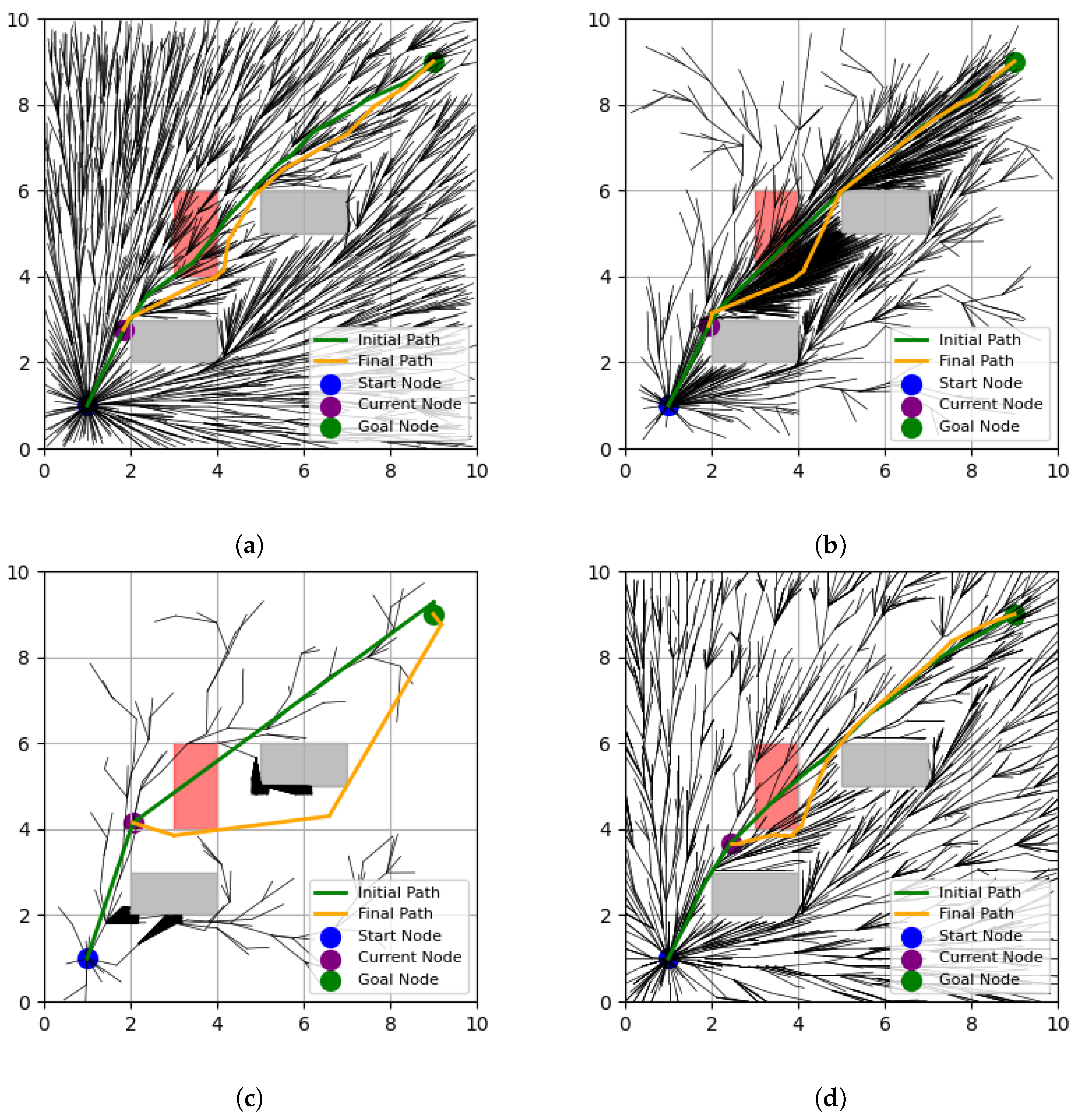
In practice, when designing global path planning (GPP) algorithms, the environment is typically assumed to be static, and the GPP algorithm is developed under this assumption. Any dynamic changes in the environment are usually addressed through Local Path Planning (LPP). However, when incorporating dynamic environments into GPP operations, it is common to recompute the global path whenever environmental changes are detected. This approach ensures that the system adapts to the new environment by generating an updated global path and continuing operations accordingly. Specifically, the system initially operates based on a pre-computed global path while periodically monitoring for environmental changes. Upon detecting such changes, the system recomputes the global path and subsequently performs LPP to handle finer adjustments within the updated environment. A detailed discussion of related studies addressing this approach can be found in the Related Words Section of this paper.

6. Conclusions

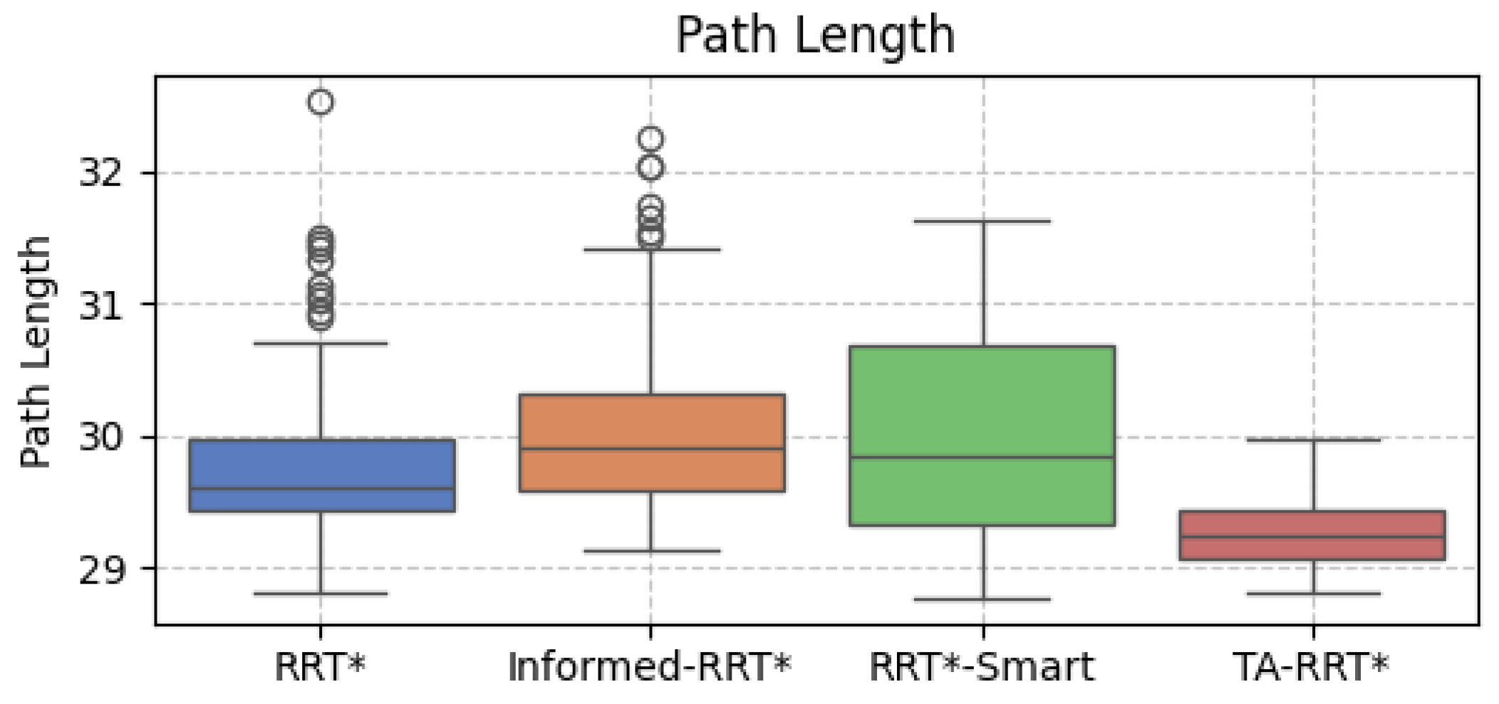
In this paper, we proposed a terrain analysis-based adaptive RRT* (TA-RRT*) algorithm to address the path planning problem. The proposed algorithm enables efficient path exploration by analyzing the complexity of terrain and employing density-based sampling using the terrain corners. Notably, TA-RRT* demonstrated the ability to effectively optimize its initial path, even in complex environments. The experimental results showed superior performance in terms of path length compared to conventional RRT* algorithms, and it produced more consistent results. The proposed TA-RRT* algorithm demonstrated its robustness through path replanning in dynamic scenarios, effectively navigating changing conditions with reliable performance.

In future research, we plan to improve the performance of the proposed algorithm by applying it to various operational environments and platforms. Through this, we aim to improve the algorithm’s versatility and allow it to maintain consistent performance in various conditions.

References

1. Wang, J.; Li, T.; Li, B.; Meng, M.Q.H. GMR-RRT*: Sampling-based path planning using gaussian mixture regression. IEEE Trans. Intell. Veh. 2022, 7, 690–700. [Google Scholar] [CrossRef]
2. Kim, Y.G.; Chang, W.; Kim, K.; Oh, T. Development of an Autonomous Situational Awareness Software for Autonomous Unmanned Aerial Vehicles. J. Aerosp. Syst. Eng. 2021, 15, 36–44. [Google Scholar]
3. Qi, J.; Yang, H.; Sun, H. MOD-RRT*: A Sampling-Based Algorithm for Robot Path Planning in Dynamic Environments. IEEE Trans. Ind. Electron. 2020, 68, 7244–7251. [Google Scholar] [CrossRef]
4. Chang, W.; Lee, S.; Kim, Y.-G.; Oh, T. Autonomous Mission Management Software Design and Verification Technique for Unmanned Aerial Vehicles. J. Korean Soc. Aeronaut. Space Sci. 2021, 49, 505–513. [Google Scholar]
5. Oh, T.; Yoon, H.-S. A Fault Management Design of Dual-Redundant Flight Control Computer for Unmanned Aerial Vehicle. J. Korean Soc. Aeronaut. Space Sci. 2022, 50, 349–357. [Google Scholar]
6. Beycimen, S.; Ignatyev, D.; Zolotas, A. A Comprehensive Survey of Unmanned Ground Vehicle Terrain Traversability for Unstructured Environments and Sensor Technology Insights. Eng. Sci. Technol. Int. J. 2023, 47, 101457. [Google Scholar] [CrossRef]
7. Tampuu, A.; Matiisen, T.; Semikin, M.; Fishman, D.; Muhammad, N. A survey of end-to-end driving: Architectures and training methods. IEEE Trans. Neural Netw. Learn. Syst. 2020, 33, 1364–1384. [Google Scholar] [CrossRef]
8. Nowakowski, M. Operational Environment Impact on Sensor Capabilities in Special Purpose Unmanned Ground Vehicles. In Proceedings of the 2024 21st International Conference on Mechatronics-Mechatronika (ME), Brno, Czech Republic, 4–6 December 2024; pp. 1–5. [Google Scholar] [CrossRef]
9. Ma, Y.; Wang, T.; Bai, X.; Yang, H.; Hou, Y.; Wang, Y.; Qiao, Y.; Yang, R.; Manocha, D.; Zhu, X. Vision-centric bev perception: A survey. arXiv 2022, arXiv:2208.02797. [Google Scholar] [CrossRef]
10. Tan, C.S.; Mohd-Mokhtar, R.; Arshad, M.R. A Comprehensive Review of Coverage Path Planning in Robotics Using Classical and Heuristic Algorithms. IEEE Access 2021, 9, 119310–119342. [Google Scholar] [CrossRef]
11. Jung, S.; Jun, W.; Oh, T.; Lee, S. Performance Analysis of Motion Planning for Outdoor Autonomous Delivery Robot. In Proceedings of the 2024 IEEE International Conference on Consumer Electronics (ICCE), Las Vegas, NV, USA, 5–8 January 2024; pp. 1–6. [Google Scholar]
12. Wang, N.; Li, X.; Zhang, K.; Wang, J.; Xie, D. A Survey on Path Planning for Autonomous Ground Vehicles in Unstructured Environments. Machines 2024, 12, 31. [Google Scholar] [CrossRef]
13. LaValle, S. Rapidly-Exploring Random Trees: A New Tool for Path Planning. Research Report 9811. 1998. Available online: http://lavalle.pl/papers/Lav98c.pdf (accessed on 15 January 2025).
14. Kavraki, L.E.; Svestka, P.; Latombe, J.C.; Overmars, M.H. Probabilistic roadmaps for path planning in high-dimensional configuration spaces. IEEE Trans. Robot. Autom. 1996, 12, 566–580. [Google Scholar] [CrossRef]
15. Karaman, S.; Walter, M.R.; Perez, A.; Frazzoli, E.; Teller, S. Anytime Motion Planning using the RRT*. In Proceedings of the 2011 IEEE International Conference on Robotics and Automation, Shanghai, China, 9–13 May 2011; pp. 1478–1483. [Google Scholar] [CrossRef]
16. Kuffner, J.; LaValle, S.M. RRT-connect: An efficient approach to single-query path planning. In Proceedings of the Proceedings 2000 ICRA. Millennium Conference. IEEE International Conference on Robotics and Automation. Symposia Proceedings (Cat. No. 00CH37065); IEEE: San Francisco, CA, USA, 2000; Volume 2, pp. 995–1001. [Google Scholar]
17. Gammell, J.D.; Srinivasa, S.S.; Barfoot, T.D. Informed RRT*: Optimal sampling-based path planning focused via direct sampling of an admissible ellipsoidal heuristic. In Proceedings of the 2014 IEEE/RSJ International Conference on Intelligent Robots and Systems; Chicago, IL, USA, 14–18 September 2014, pp. 2997–3004.
18. Nasir, J.; Islam, F.; Malik, U.; Ayaz, Y.; Hasan, O.; Khan, M.; Muhammad, M.S. RRT*-SMART: A rapid convergence implementation of RRT. Int. J. Adv. Robot. Syst. 2013, 10, 299. [Google Scholar] [CrossRef]
19. Zhao, Y.; Liu, K.; Lu, G.; Hu, Y.; Yuan, S. Path planning of UAV delivery based on improved APF-RRT* algorithm. J. Phys. Conf. Ser. 2020, 1624, 042004. [Google Scholar] [CrossRef]
20. Wang, J.; Chi, W.; Li, C.; Wang, C.; Meng, M.Q.H. Neural RRT*: Learning-based optimal path planning. IEEE Trans. Autom. Sci. Eng. 2020, 17, 1748–1758. [Google Scholar] [CrossRef]
21. Jones, M.; Djahel, S.; Welsh, K. Path-planning for unmanned aerial vehicles with environment complexity considerations: A survey. ACM Comput. Surv. 2023, 55, 1–39. [Google Scholar] [CrossRef]
22. Zhang, S.; Li, H.; Wang, M.; Liu, M.; Chen, P.; Lu, S.; Liu, S.; Murugesan, K.; Chaudhury, S. On the Convergence and Sample Complexity Analysis of Deep Q-Networks with ϵ-Greedy Exploration. In Proceedings of the Advances in Neural Information Processing Systems; Curran Associates, Inc.: New Orleans, LA, USA, 2023; Volume 36, pp. 13064–13102. [Google Scholar]
23. Harris, C.; Stephens, M. A combined corner and edge detector. In Proceedings of the Alvey Vision Conference, Manchester, UK, 31 August–2 September 1988; Volume 15, pp. 10–5244. [Google Scholar]
24. Pal, P.; Sato, K. A comprehensive review on convex and concave corners in silicon bulk micromachining based on anisotropic wet chemical etching. Micro Nano Syst. Lett. 2015, 3, 6. [Google Scholar] [CrossRef]
25. Maneewongvatana, S.; Mount, D.M. It’s okay to be skinny, if your friends are fat. In Proceedings of the Center for Geometric Computing 4th Annual Workshop on Computational Geometry, Baltimore, MD, USA, 15–16 October 1999; Volume 2, pp. 1–8. [Google Scholar]
26. Hwang, J.J.; Xu, R.; Lin, H.; Hung, W.C.; Ji, J.; Choi, K.; Huang, D.; He, T.; Covington, P.; Sapp, B.; et al. Emma: End-to-end multimodal model for autonomous driving. arXiv 2024, arXiv:2410.23262. [Google Scholar]
27. Lan, G.; Hao, Q. End-To-End Planning of Autonomous Driving in Industry and Academia: 2022–2023. arXiv 2023, arXiv:2401.08658. [Google Scholar]
28. Shalev-Shwartz, S. On a formal model of safe and scalable self-driving cars. arXiv 2017, arXiv:1708.06374. [Google Scholar]
29. Philion, J.; Fidler, S. Lift, splat, shoot: Encoding images from arbitrary camera rigs by implicitly unprojecting to 3d. In Proceedings of the Computer Vision–ECCV 2020: 16th European Conference, Glasgow, UK, 23–28 August 2020; Proceedings, Part XIV 16. Springer: Berlin/Heidelberg, Germany, 2020; pp. 194–210. [Google Scholar]
30. Ma, X.; Liu, S.; Xia, Z.; Zhang, H.; Zeng, X.; Ouyang, W. Rethinking pseudo-lidar representation. In Proceedings of the Computer Vision–ECCV 2020: 16th European Conference, Glasgow, UK, 23–28 August 2020; Proceedings, Part XIII 16. Springer: Berlin/Heidelberg, Germany, 2020; pp. 311–327. [Google Scholar]
31. Moezzi, R.; Krcmarik, D.; Hlava, J.; Cỳrus, J. Hybrid SLAM modelling of autonomous robot with augmented reality device. Mater. Today Proc. 2020, 32, 103–107. [Google Scholar] [CrossRef]
32. Yang, B.; Pham, T.M.T.; Yang, J. Evaluating and Improving the Robustness of LiDAR-based Localization and Mapping. arXiv 2024, arXiv:2409.10824. [Google Scholar]
33. Yin, J.; Li, L.; Mourelatos, Z.P.; Liu, Y.; Gorsich, D.; Singh, A.; Tau, S.; Hu, Z. Reliable Global Path Planning of Off-Road Autonomous Ground Vehicles Under Uncertain Terrain Conditions. IEEE Trans. Intell. Veh. 2023, 9, 1161–1174. [Google Scholar] [CrossRef]
34. Dong, H.; Gu, W.; Zhang, X.; Xu, J.; Ai, R.; Lu, H.; Kannala, J.; Chen, X. Superfusion: Multilevel Lidar-Camera Fusion for Long-Range HD Map Generation. In Proceedings of the 2024 IEEE International Conference on Robotics and Automation (ICRA), Yokohama, Japan, 13–17 May 2024; pp. 9056–9062. [Google Scholar] [CrossRef]
35. Yu, J.; Zhang, Z.; Xia, S.; Sang, J. ScalableMap: Scalable Map Learning for Online Long-Range Vectorized HD Map Construction. arXiv 2023, arXiv:2310.13378. [Google Scholar]
36. Arnold, E.; Dianati, M.; de Temple, R.; Fallah, S. Cooperative Perception for 3D Object Detection in Driving Scenarios Using Infrastructure Sensors. IEEE Trans. Intell. Transp. Syst. 2020, 23, 1852–1864. [Google Scholar] [CrossRef]
37. Xu, R.; Tu, Z.; Xiang, H.; Shao, W.; Zhou, B.; Ma, J. CoBEVT: Cooperative Bird’s Eye View Semantic Segmentation with Sparse Transformers. arXiv 2022, arXiv:2207.02202. [Google Scholar]
38. Wang, T.-H.; Manivasagam, S.; Liang, M.; Yang, B.; Zeng, W.; Urtasun, R. V2VNet: Vehicle-to-Vehicle Communication for Joint Perception and Prediction. In Proceedings of the 16th European Conference on Computer Vision (ECCV), Glasgow, UK, 23–28 August 2020; pp. 605–621. [Google Scholar] [CrossRef]
39. Qiao, D.; Zulkernine, F. Adaptive Feature Fusion for Cooperative Perception Using Lidar Point Clouds. In Proceedings of the IEEE/CVF Winter Conference on Applications of Computer Vision (WACV), Waikoloa, HI, USA, 2–8 January 2023; pp. 1186–1195. [Google Scholar] [CrossRef]
40. Wang, B.; Zhang, L.; Wang, Z.; Zhao, Y.; Zhou, T. CORE: Cooperative Reconstruction for Multi-Agent Perception. In Proceedings of the IEEE/CVF International Conference on Computer Vision (ICCV), Paris, France, 2–6 October 2023; pp. 8710–8720. [Google Scholar]
41. Coulter, R.C. Implementation of the Pure Pursuit Path Tracking Algorithm; Technical Report; Carnegie Mellon University: Pittsburgh, PA, USA, 1992. [Google Scholar]
42. Thrun, S.; Montemerlo, M.; Dahlkamp, H.; Stavens, D.; Aron, A.; Diebel, J.; Fong, P.; Gale, J.; Halpenny, M.; Hoffmann, G.; et al. Stanley: The Robot That Won the DARPA Grand Challenge. In The 2005 DARPA Grand Challenge: The Great Robot Race; Springer: Berlin/Heidelberg, Germany, 2007; pp. 1–43. [Google Scholar]
Figure 1. Example of RRT* path planning results.
Applsci 15 02287 g001
Figure 2. Example of corner detection on a grid, with stars marking g ( x , y ) and ‘X’ symbols indicating value discrepancies with neighboring grids. (a) Convex corner, (b) edge region, and (c) concave corner.
Applsci 15 02287 g002
Figure 3. Examples of (a) the corner detection result, where red points represent identified corners, and (b) the PDF derives from the result of (a).
Applsci 15 02287 g003
Figure 4. Example of (a) the search result for corners within the radius of the reference point using a KD tree. (b) The tree structure of the KD tree.
Applsci 15 02287 g004
Figure 5. Example of adaptive step size according to density.
Applsci 15 02287 g005
Figure 6. Examples of path planning results in a simple environment. (a) RRT*. (b) Informed-RRT*. (c) RRT*-Smart. (d) TA-RRT*. The blue and green dots represent the start and goal points, and the purple line represents the resulting path.
Applsci 15 02287 g006
Figure 7. Box plots expressing the path length distributions of the path planning algorithms in a simple environment.
Applsci 15 02287 g007
Figure 8. Examples of path planning results in an intermediate environment. (a) RRT*. (b) Informed-RRT*. (c) RRT*-Smart. (d) TA-RRT*. The blue and green dots represent the start and goal points, and the purple line represents the resulting path.
Applsci 15 02287 g008
Figure 9. Box plots expressing the path length distributions of the path planning algorithms in an intermediate environment.
Applsci 15 02287 g009
Figure 10. Examples of path planning results in complex environments. (a) RRT*. (b) Informed-RRT*. (c) RRT*-Smart. (d) TA-RRT*. The blue and green dots represent the start and goal points, and the purple line represents the resulting path.
Applsci 15 02287 g010
Figure 11. Box plots expressing the path length distributions of the path planning algorithms in complex environments.
Applsci 15 02287 g011
Figure 12. Examples of path replanning results in dynamic scenarios #1. (a) RRT*. (b) Informed-RRT*. (c) RRT*-Smart. (d) TA-RRT*.
Applsci 15 02287 g012
Figure 13. Examples of path replanning results in a dynamic scenario #2. (a) RRT*. (b) Informed-RRT*. (c) RRT*-Smart. (d) TA-RRT*.
Applsci 15 02287 g013