Article

A Predictive Multibody Model of Paper Applied to Cash Recycling

by
Lorenzo Giorio
1,†,
Chiara Gastaldi
2,*,†,
Cristiana Delprete
2,†,
Samuele Libetti
3,† and
Davide Eleuteri
3,†
1
Department of Management and Production Engineering—DIGEP, Politecnico di Torino, Corso Duca degli Abruzzi 24, 10129 Torino, Italy
2
Department of Mechanical and Aerospace Engineering—DIMEAS, Politecnico di Torino, Corso Duca degli Abruzzi 24, 10129 Torino, Italy
3
Sesami, Via Statale 17, 10012 Bollengo, Italy
*
Author to whom correspondence should be addressed.
These authors contributed equally to this work.
Appl. Sci. 2025, 15(5), 2283; https://doi.org/10.3390/app15052283
Submission received: 6 January 2025 / Revised: 10 February 2025 / Accepted: 13 February 2025 / Published: 20 February 2025

Abstract

:
Despite the spread of digital payment systems, banknotes still play a vital role in the lives of people, financial institutions, and businesses. Automation is crucial in all cases where a large number of deposits/withdrawals need to be handled. In spite of the large number of cash recyclers worldwide and their continuous evolution, one of the most significant parts of their design, i.e., the interaction with banknotes, is still predominantly based on a lengthy iterative process that includes testing. This has detrimental effects not only on time-to-market but also on the costs and on the willingness to explore multiple design solutions, thus potentially reducing the quality of the final product. The testing phase is made necessary by the lack of an effective and predictive model for the banknote and of its contact with the components of the cash recycler. The purpose of this work is to bridge this gap in the literature by introducing and validating an original multibody model of the banknote-cash recycler system. The proposed approach includes the possibility of including the nonlinear orthotropic paper material curves and of customizing quantities such as paper thickness and friction coefficients at specific locations, with potential applications in optimizing banknote validation, reducing wear in cash handling systems, and improving the design of next-generation cash recyclers.

1. Introduction

Although digital payment methods are becoming increasingly popular, cash continues to be a common payment choice. In the United States, 83% of households with incomes greater than $85,000 use cash monthly [1]. Moreover, even countries working to reduce cash often find it necessary to retain that infrastructure to properly handle upsurges of cash during emergencies [2]. As automation, artificial intelligence, and facial recognition become increasingly popular, and fewer cashiers are employed, the future of cash usage may become strongly linked to cash recyclers, not only at bank locations but also at retail businesses. A cash recycler is a complex machine that automates the simple yet important tasks of accepting and dispensing cash. It also stores money securely at the point of use and keeps an accurate account of the cash on hand. In a cash recycler, banknotes are placed into a feeder and then passed through a bill identifier to determine the denomination and validity of the notes [3]. The banknotes are then stored in separate cassettes or modules for dispensing in future transactions. The expected performance of a cash recycler is subject to increasing demands, e.g., seven banknotes handled per second, one at a time, without tearing.
In this context, a computer-aided methodology to simulate the process of transporting banknotes through the cash recycler would be particularly beneficial. The presence of such a design simulation tool can be a great competitive advantage for companies. With a working methodology available, it would be possible to simulate banknote transport in different construction solutions without the need to physically build prototypes, thus reducing costs and product development time.
Another advantage of simulation is the ability to investigate the behavior of the system under operating conditions that are not easily replicated experimentally. This includes analyzing the behavior of the banknote with a microsecond resolution, which is not feasible even with the use of powerful high-speed cameras. The numerical approach then leads to a better and deeper understanding of the physical phenomena underlying paper transport, thus paving the way to an effective process optimization. The tool can thus serve as a guide to the entire development process of machines that handle cash.
In the literature, studies and computational models of the material behavior of paper and paperboard at different scales have been published [4,5], as well as models considering the mechanical behavior of paper-based components, such as paperboard boxes [6,7,8]. To the authors’ knowledge, however, there are no models available that consider paper sheets as components within more complex mechanical systems, e.g., a cash recycler, and therefore allow the interaction of paper with other mechanical components to be simulated.
The objective of the present paper is to propose a methodology to simulate banknote transport in a Multibody (MB) framework. This task requires an effective model for the banknote. In the literature, models of paper sheets in a MB context are often limited to 1D simplified models [9], and while options to introduce flexible bodies in a MB simulation are available [10,11,12], they do not meet all the necessary requirements, as detailed in the following section.
This paper proposes an original modeling strategy to correctly replicate the flexible orthotropic behavior of paper [13], while ensuring a robust description of the contact [14] between the banknote and the various components of the cash recycler. The methodology created will not be limited to a specific application, but it will be possible to implement it in any system in which a sheet of paper, such as a banknote, is to interact. Another strong feature of the proposed methodology is the possibility to implement it in a commercial MB software.
The work is organized as follows. Section 2 defines the requirements needed to obtain an effective model of the banknote itself. Section 2.1 reviews the existing strategies used to model flexible bodies to highlight how not all requirements for banknote modeling are met. A new method meeting all requirements is presented and tuned in Section 2.2. Section 3 focuses on the representation of the contact between the banknote and the different components of the cash recycler. The results, coming both from a simplified and a high-fidelity model of a cash recycler, are presented and discussed in Section 4. Conclusions and main achievements are summarized in Section 5.

2. Modeling the Banknote

Building a MB model of a banknote, or of any paper sheet, being transported through a machine requires a series of features.
The banknote, considered to be made of paper, is a flexible body which deforms simply due to the effect of gravity. In fact, it is precisely its flexibility, i.e., the first requirement of the banknote MB model, that allows it to be transported through the cash recycler.
In addition to the complexity of having to model the banknote as a flexible body, another challenge is its nonlinear material behavior. As already discussed in the previous section and further shown in [13], paper exhibits a nonlinear stress–strain curve, i.e., Young’s modulus dependent on the strain level. Furthermore, paper exhibits anisotropic behavior, but is generally simplified as an orthotropic material.
In detail, physical properties vary along the following three mutually perpendicular directions shown in Figure 1: the machine direction MD, the cross-machine direction CD, and the out-of-plane direction ZD, that is, along the thickness.
It is obvious that the inclusion of such a body in a MB simulation increases its complexity both in terms of modeling and computational time. Although this scenario will not be directly discussed in the paper, having the possibility to effectively model the behavior of paper under a significant amount of stress/strain may be crucial when evaluating possible damages to the banknote during transport. A faithful representation of the nonlinear orthotropic material behavior of paper is therefore set as the second requirement of the MB model. The third requirement is having an efficient and effective model for the contact between the banknote itself and the different components of the cash recycler. The fourth and final requirement focuses on the simplicity of creating the banknote model. In particular, we hope to minimize the user’s execution of repetitive functions and to minimize pre-processing in general. The following paragraphs focus on existing methodologies which may be applicable to banknote MB modeling. Their pros and cons will be discussed, and the need to develop a new methodology will be highlighted.

2.1. State-of-the-Art Methodologies Used to Represent Flexible Bodies in MB Simulations

The MB simulation of a system consisting of rigid bodies is now a mature technology. The representation of flexible bodies and, furthermore, their contacts are, however, quite complex and can vary, albeit with some common methodologies, among different software. The most common types of flexible body supported by most commercial software are the following:
  • Linear flexible (LF) body obtained through a component mode synthesis (CMS) condensation method;
  • Non linear finite element (NLFE) body.
These methodologies, which have the merit of being readily available in most commercial MB software, such as the Altair MotionSolve© suite, version 2023.1, have limitations. The pros and cons will be discussed in detail in the following paragraphs.

2.1.1. Linear Condensation

Modeling the dynamic behavior of a MB system is characterized by a composition of rigid bodies, interconnected by joints, springs, dampers, and actuators. The finite element (FE) method is not directly scalable, and MB modeling often relies on too crude approximations of the properties of the bodies and their interaction. An obvious solution to this issue, especially when the bodies that need to be simulated are flexible, is to integrate FE and MB analyses. In this way, condensed elastic sub-models can be easily transferred from the FE software to the MB software, and dynamic loads can be transferred back from the MB software to the FE software.
To make this strategy computationally feasible, model order reduction techniques are applied to the FE model of each flexible substructure. In this context, the most common choice is CMS [15,16,17,18,19]. In practice, interface nodes, also called ‘master’ nodes, which are points of connection of the flexible body with other entities, are distinguished from all other nodes, called ‘slave’ nodes. These CMS methods can be divided into those which employ free-interface normal modes and attachment modes [17,18,19] and those using fixed-interface normal modes and constraint modes [15,16]. In both cases, the normal modes are used to build a modal transformation matrix which filters out insignificant high-frequency vibration modes, thus reducing the problem’s dimensionality. While the first requirement of the banknote model, detailed in Section 2, i.e., flexibility, is satisfied, the application of CMS methods is not free from difficulties, such as the appropriate selection of modes that can appropriately describe the deformation field of a flexible body and therefore guarantee an accurate reduction [20].
It should be stressed that, in all sub-structuring techniques, the modes’ computation is, by its nature, linear. Even recently introduced condensation methods which attempt to capture structures subjected to friction contact [21,22,23] do so by a collection of linear modes pertaining to the structures with specifically chosen boundary conditions on the contact interface. It is possible, therefore, to generate flexible bodies with a linear behavior alone, i.e., the second requirement from Section 2 is not satisfied.
The biggest limitation that makes sub-structuring unsuitable for the simulation of paper sheet transport, however, is the definition of contact, i.e., third requirement from Section 2. The contact between a flexible body and another body, either rigid or flexible, is modeled using the contact entity ‘Point on deformable surface’ [24,25]. Specifically, the contact occurs between a sphere of radius r and a deformable surface attached to the flexible body; an example is shown in Figure 2. The sphere belongs to the second body in contact. As in the present case, multiple spheres may be defined to correctly describe the geometry of the second body in contact. Due to the way the deformable surface is designed, it requires that the center of the sphere always lie within the area described by the surface. If this condition is not met, the solver forces the coordinates of the point at the extremes of the deformable surface ranges until it actually falls within them. The problem is that this condition may never occur, as the banknote moves in the MB, and with it, the deformable surface; the consequence is that the analysis may not converge, and it may fail.
Another limitation of sub-structuring techniques is pre-processing, i.e., the reduction phase which would make modifications to the banknote model cumbersome, i.e., fourth requirement from Section 2.

2.1.2. Nonlinear Finite Elements

The second strategy to generate a flexible body in a MB simulation software such as MotionSolve© is the NLFE approach. Unlike the previously discussed CMS strategy, no modal representation is necessary, as the body is discretized using ad hoc FE formulation. Although 3D NFLE have been proposed for specific applications [26], only 1D and 2D elements are available in MB simulation software [27]. In the specific case of MotionSolve©, it is emphasized how only 1D body modeling is easily implemented, while the use of 2D shells would require specific user-developed coding. It is clear how the adoption of 1D or 2D elements is not sufficient to effectively model the orthotropic behavior of paper material (i.e., second requirement from Section 2). Furthermore, only specific constitutive laws are available in the software library, e.g., hyper-elastic models (Neo-Hookean, Mooney–Rivlin, and Yeoh).
Once again, the definition of the contact between the NLFEs and a second body suffers from all the limitations detailed in Section 2.1, i.e., the third requirement is once again not met.
It is therefore clear that the limitations listed above make the NLFEs currently implemented in commercial software a sub-optimal choice for paper (and banknote) modeling.

2.2. Methodology

To overcome the limitations highlighted in the previous section, a new strategy has been developed completely from scratch. The banknote body is discretized into a multitude of rigid bodies, connected together with springs and dampers. A rigid body, by definition, does not deform; therefore, it might seem counter-intuitive to use rigid bodies to represent a flexible, deformable body. In other words, flexibility is transferred from the ‘bodies’ to the ‘connections’, i.e., spring and damper.
It is clear how a finer discretization leads to a better representation of the flexibility of the banknote, at the cost of a larger computational time. A trade-off must therefore be sought, as discussed in Section 4.4. Another important modeling choice is the position of the connections. In this context, two configurations have been analyzed as follows:
  • The connections (spring+damper) are placed between the centers of mass of neighboring ‘boxes’, hereafter termed ‘center-to-center’;
  • The spring/damper connect the corners of neighboring boxes, as shown in Figure 3, hereafter termed ‘edge-to-edge’.
Both methods will be presented, together with the tuning methodology, to determine the connections’ characteristic values. Pros and cons of both methods will be highlighted and discussed.

2.2.1. Tuning Procedure

Considering the banknote placed on the x y plane, springs with k x stiffness connect two boxes along the X direction and springs with k y stiffness connect the boxes along the Y direction. A schematic is shown in Figure 4.
A translational k z spring connects adjacent boxes to resist out-of-plane motion. In the center-to-center connection, one spring per typology connects the mass centers, while in the edge-to-edge connection two springs per typology are necessary. Given the small thickness of the banknotes (about 0.1 mm), it is sufficient to use only one layer. In addition to the translation springs, it is necessary to include rotational springs with stiffnesses k t x , k t y , and k t z , which act with a resisting torque when a relative rotation is created between the boxes, as shown in Figure 4. In practice, the connection between rigid bodies in the MotionSolve© software is made using the ‘Bushing’ entity, which allows translation and rotation stiffnesses, and the associated damping, to be entered.
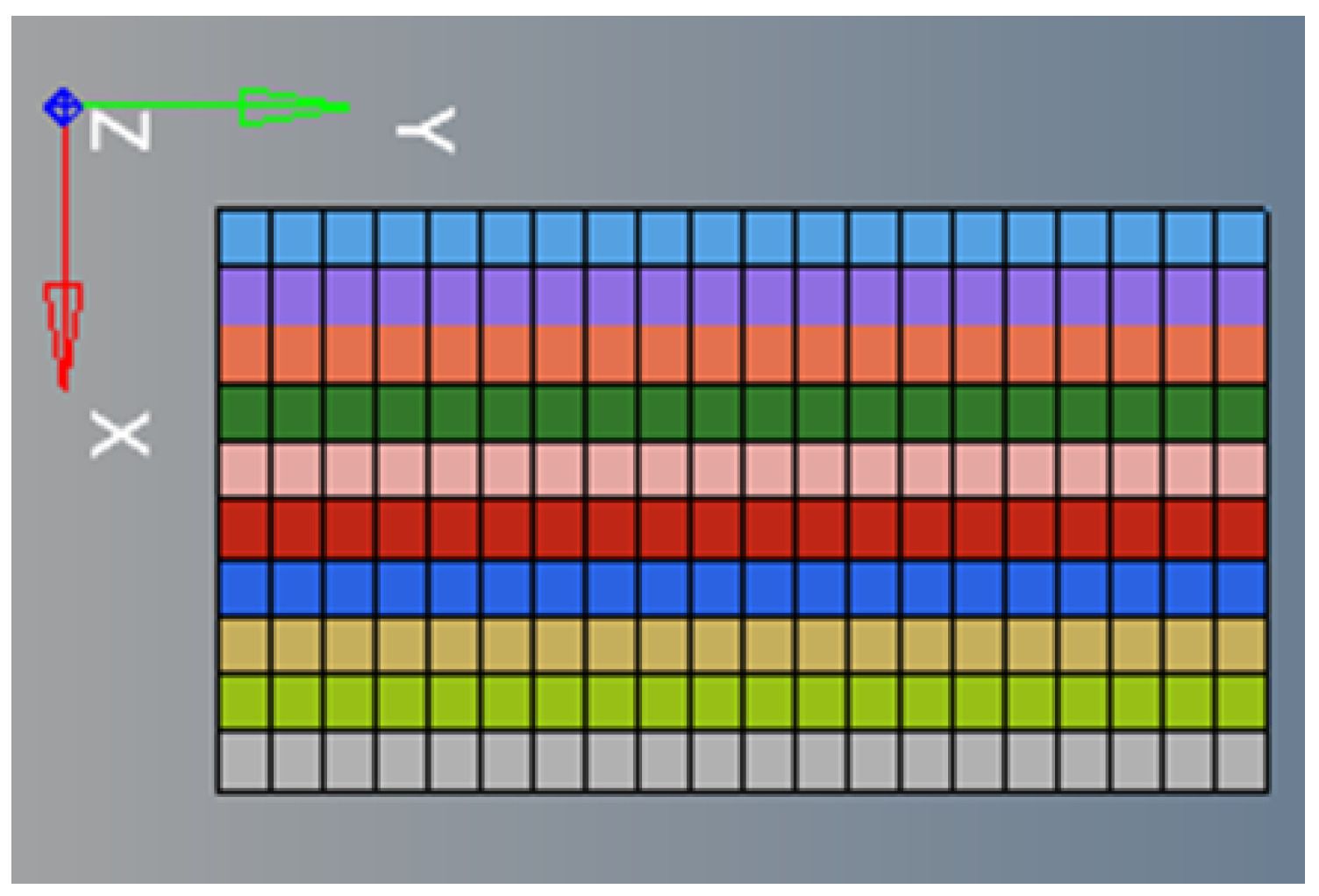
A value must be assigned to each of the above stiffnesses. The specific values depend on the chosen discretization and on the configuration (i.e., number of springs of the center-to-center vs. edge-to-edge layout). As an example, let us consider a EUR 10 banknote (67 mm × 127 mm × 0.1 mm), shown in Figure 5, discretized in n x = 10 boxes along the X direction and n y = 20 boxes along the Y direction.
Starting from the mass and dimension of the banknote and the chosen discretization (variables n x and n y ), it is possible to define the following quantities:
  • The dimension of the boxes
    d x = L x n x 1 , d y = L y n y 1 ,
  • The mass of each box
    m = M n x · n y ,
  • The section of each box normal to directions X and Y
    A x = d y · s , A y = d x · s .
All relevant quantities are reported in Table 1.
The values of the translation stiffnesses k x and k y are obtained from the stress–strain curves of the paper. In detail, with reference to the chosen orientation of the banknote (see Figure 5), k x may be obtained from the stress–strain curve obtained in machine direction MD, while k y may be obtained from the tensile test performed in cross direction CD (see Figure 1). The data presented here are taken from [13].
Considering the machine direction MD, i.e., X direction, and the center-to-center configuration, the stress–strain relation can be expressed as follows:
σ = E M D · ϵ = k x · Δ L A x ,
where the strain is defined as ϵ = Δ L / L 0 = Δ L / d x .
By substituting the definition of ϵ into Equation (4) as follows:
k x = E M D · A x d x ,
and similarly, one can define k y as follows:
k y = E C D · A y d y .
In the simulation, one may chose to use as Young’s Modulus along the different directions ( E M D and E C D ), a mean value valid for all strains, or feed MotionSolve© with the nonlinear stress–strain curves. In the edge-to-edge configuration, the single k x and k y values will be 50% of their center-to-center counterpart; however, the global stiffness will be the same. In detail, considering the X direction as an example, the connections on the outer edges of the banknote will be linked by a k x spring, while the inner ones will be linked by a 2 k x spring. The value of the k z spring is chosen to be one order of magnitude higher than that of k x and k y to prevent limiting out-of-plane motion between neighboring boxes.
Dampings c x and c y are derived from the mass and stiffness information, applying the single mass-spring-damper system as follows:
c x = 2 ξ k x · m , c y = 2 ξ k y · m ,
where ξ is the relative damping coefficient and depends on the material, k x is the stiffness, and m is the mass of a box.
The damping coefficient should be derived from experimental measurements and by the logarithmic decrement method. Since such tests are not available, relative damping ξ = 12% was chosen, assuming that paper has greater damping than steel, for which a coefficient of 3–5% is typically used. In addition, coefficients of 15–20% are assumed for wooden structures, and paper is a material that is produced from it, so the value of 12% is reasonable.
The rotational springs were calibrated by reproducing in simulation the experimental tests described below. To calibrate k t x , a test was performed by keeping the short side fixed and letting the banknote drop by gravity, as shown in Figure 6. The displacement of the free side is measured with a probe. The displacement of the free side measured experimentally is 60.76 mm. The MB model that reproduces the experimental condition consists of the banknote, decomposed into 200 boxes, with fixed joints on one of the short sides. The rotational springs k t x are the only ones activated in this condition. The simulation was run iteratively with different tentative values of k t x , and the resulting contour plot (lower portion of Figure 6) was compared with the experimentally measured displacement. In this context, one must then consider errors in the experimental measurement and the fact that the simulation may not perfectly represent the experimental boundary conditions. In fact, the size of the boxes limits the precision with which one can emulate the portion of the banknote which is fixed. Assigning the value k t x = 0.27 N mm/rad for the center-to-center configuration yields a simulated free side displacement of 60.26 mm; in light of the considerations just made this can be considered acceptable. The relative damping coefficient used is once again used ξ = 12% together with Equation (7) to define c t x . A further confirmation of the adequacy of the ξ estimate is the fact that the number of oscillations observed in the contour plot matches those observed experimentally.
A similar procedure was performed to estimate k t y and c t y . The procedure was repeated with the edge-to-edge configuration, yielding consistent results.
The values of the translation and rotation stiffness values with associated damping are summarized in Table 2 for the two configurations. It is emphasized that the rotational stiffness k t z was not calibrated based on experimental tests but was assumed to be high enough to prevent the rotation of two adjacent boxes around the Z axis.

2.2.2. Automated Implementation

The proposed methodology, i.e., discretizing the banknote into rigid bodies, has great potential because it offers complete control over the model; however, its implementation requires heavy user involvement. In MotionView©, there is no automatic operation to create a grid of rigid bodies, bushings, graphical elements, etc. It is possible to import a text or excel file with a table containing the coordinates of the points, but these would then remain fixed in space since the coordinates are represented by numbers and not variables. Performing the necessary operations ‘by hand’ is not feasible, as the banknote system consists of hundreds or thousands of entities.
Thus, the implementation of the proposed methodology has to be automated in some way. This is achieved by the combined use of the MDL and Python languages. The MDL language makes it possible to write in a text file the entities to be included in a MB model; therefore, mouse-click operations can be avoided by simply importing a MDL file. The creation of repetitive lines of text is automated with the Python programming language. Specifically, different Python codes are created to generate the following:
  • The points at the center and corners of each rigid body and the rigid bodies mass and inertia properties;
  • The graphical elements to be associated with each body, i.e., a box; these graphics have both visualization purposes in post-processing but also play a key role in defining contacts;
  • The connecting entities between all rigid bodies, i.e., bushing;
  • A deformable surface that attaches to each rigid body at its midpoint in the midplane; this code is optional and is used to visualize results.
All the characteristic quantities of the entities that make up the banknote have been parameterized with variables. For example, it is possible to change the mass of the banknote, and thus that of all rigid bodies, by changing the relative variable, just as it is possible to change the values of the stiffness constants of the bushing entities.

3. Modeling the Contact

Two types of approaches are made available in MotionSolve© to model the contacts. If the bodies involved in the contact are flexible, e.g., banknote model produced with dynamic condensation or NLFE, the contact entity to be used is the so-called ‘Point to Deformable Surface’. This contact definition strategy proved to be unsuitable to model paper transportation due to convergence problems, as discussed in Section 2. If on the other hand, the bodies involved in the contact are rigid, as in the banknote model proposed in this work, the ‘3D Rigid to Rigid Contact’ entity has to be used. This last methodology, which is more robust from a convergence point of view, will be explored in the following paragraphs.

3.1. Contact Detection

The first step is contact detection, which can be performed according to the following two approaches:
  • Analytical: Geometries are represented exactly by mathematical functions;
  • Mesh-based: The geometries are discretized more or less finely with a mesh of first-order triangular elements; in this case, one can choose whether to evaluate the displacements, velocities, and contact forces at the nodes or at the centers of the elements.
When the geometries of two bodies compenetrate, contact occurs and MotionSolve© calculates the forces that the two bodies exchange. It is obvious that the analytical approach is more precise since the compenetration is precisely detected and does not depend on the quality of the mesh, and it is also much faster. The problem is that this method can be applied only for simple geometries, for example, for cylinder-to-cylinder contact.
In general, to model the contact between the banknote and bodies with different geometries, the approach to be used will necessarily be mesh-based. However, this does not preclude the possibility of applying the analytical method for contacts between boxes and cylinders, which may represent the rollers of the cash recycler. Whenever possible, CAD geometries should be simplified to limit the computational time.
If, on the other hand, one cannot do it without using complex geometries, and thus the mesh-based approach, it is still possible to adopt strategies to limit the computational effort, while a fine mesh is required to ensure accurate results, the mesh refinement should be limited to the contact area. Furthermore, in the solver options, one may choose to take into account either the centers of the elements or the nodes. In the latter case, more contact points will be available, and thus, the results will be more accurate.
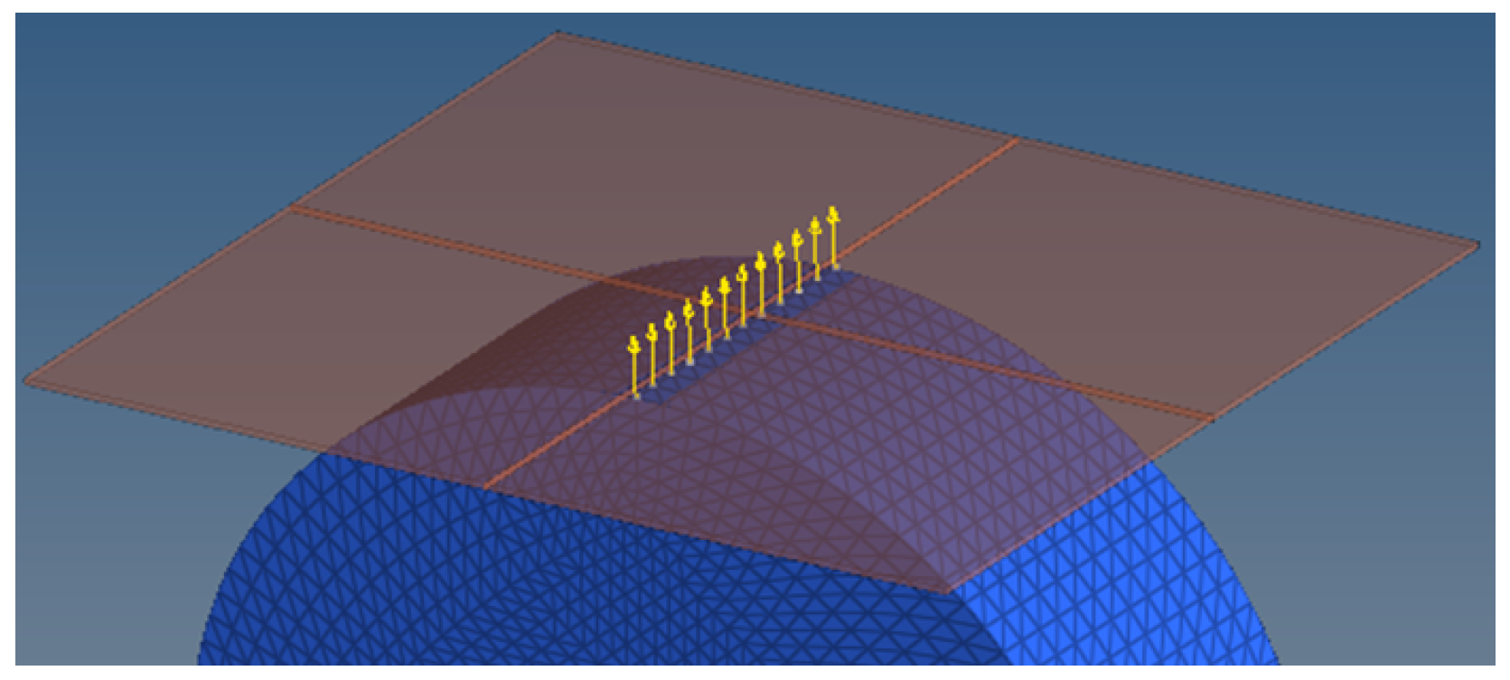
The example in Figure 7 shows four boxes resting on a cylinder. The contact area is a line, and the forces are evaluated at the nodes of the cylinder mesh, which is here defined as the master surface as it is the one with the finer discretization.

3.2. Contact Forces Computation

The second step is the calculation of the contact forces, which always occur when the penetration depth z is less than zero, being defined as the distance between two geometries, which is always positive and different from zero when the bodies are not in contact, as follows:
F N = 0 if z 0 , f ( z , z ˙ ) if z < 0 .
The Poisson model is chosen to compute the normal force, which is composed of an elastic part, responsible for repelling bodies, and a damping part, responsible for dissipating energy, as follows:
F N = F s p r i n g + F d a m p .
The elastic component is defined as follows:
F s p r i n g = k z 3 ,
where k represents the contact stiffness and depends on the materials of the two bodies.
Generally, k is chosen according to the value of interpenetration that is to be allowed as follows: the smaller the allowable z quantity, the greater the stiffness k must be.
The damping component is defined as follows:
F d a m p = F s p r i n g ( 1 c R 2 ) ( 1 + c R 2 ) · s .
The function s brings the penetration velocity into the formula, while the parameter c R is the coefficient of restitution, defined as the ratio of the relative velocity between the bodies after contact and the velocity before contact. This coefficient can vary between zero and one as follows: a value of zero implies perfectly plastic contact, that is, the two bodies remain ‘stuck’ after contact and all energy is dissipated; a value of one implies perfectly elastic contact, that is, the two bodies bounce back after contact and all energy is conserved.
Finally, the formula for the frictional force is Coulomb’s law, expressed as follows:
F d a m p = F N · μ ,
where μ is the friction coefficient between the two bodies in contact.
The specific values of k, c R , and μ need to be calibrated based on the material and on the specific model/interaction between the bodies in contact. The values used in the simulations presented in this work will be discussed in Section 4.

3.3. Contact Implementation and Automation

To conclude the modeling of the contact between rigid bodies, mention must again be made of the MDL and Python languages, which made it possible to define the thousands of contact entities between the boxes, which make up the banknote, and all the other bodies in the system. A banknote discretized in 200 boxes and in contact with four cylinders, for example, involves the definition of 800 contacts in total, because it is necessary to represent the contact between each box and all other bodies in the system. A Python v3.12.0 code has been developed to define, in an MDL file, all the contact entities between the banknote boxes and another body, which can simply be entered with its ‘variable name’ adopted in the MB model. In addition, the contact force parameters such as stiffness, coefficient of restitution, friction coefficient, etc., have been entered into the MB model as variables. Furthermore, it may be possible to define different variables such as the friction coefficient, depending on the box location (e.g., metallic stripe vs. lithography location).

4. Results and Discussion

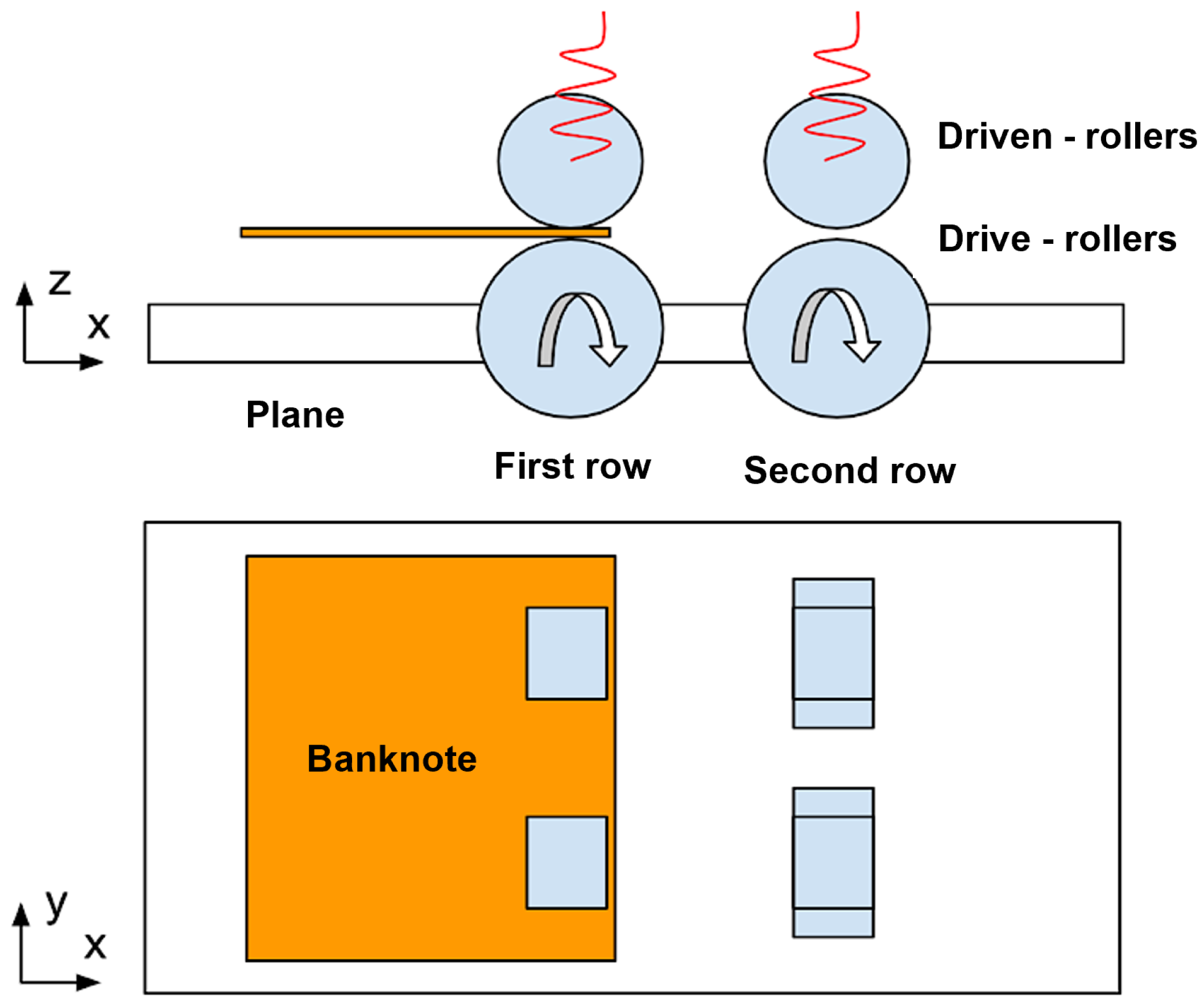
A series of simulations were performed both on a simplified model and on a high-fidelity model of a cash recycler. The simplified MB system is composed of a support plane and rollers, as shown in Figure 8. Such a model represents the transport mechanism in different parts of the cash recycler.
These simulations serve to demonstrate how the banknote, decomposed into rigid bodies, actually functions in transport and behaves as an overall flexible body. In detail, three different simulations have been performed as follows:
  • Model with four motor-rollers and four counter-rollers: The goal is to verify that the banknote is transported at the desired speed;
  • Model with four motor-rollers and two counter-rollers: The goal is to verify that the banknote is able to reach the second row of rollers and counter-rollers;
  • Model with tilted banknote: The goal is to verify the banknote tilt correction by changing roller speeds on the second row.
These three models share the same fundamental components and features. The main dimensions and mass of the components are outlined in Table 3. The mass value of the support plane is reported for completeness; however, it is irrelevant since it is fixed to ground. On the other hand, the mass of the rollers is relevant, as their rotation triggers inertial effects.
A ‘Spring Damper’ entity, comprised of stiffness, damping, spring free length, and preload, is applied to each of the four counter-rollers. In a paper transport machine, pairs of rollers and counter-rollers with a compressive load applied to them are very common. The counter-roller presses on the rollers and helps generate the necessary drag force for the banknote to travel. The selected spring entity has a stiffness of 0.319 N/mm, a preload of 3.19 N, a relative damping of 5%, and a free length of 6 mm. In the software model, it is possible to exclusively specify a stiffness value for the spring. However, it is always appropriate to add damping, to avoid the computation of unrealistic oscillations. Roller dimensions and compression spring characteristics refer to actual components.
The connection of the bodies that make up the banknote has already been discussed at length in Section 2, while it is appropriate to specify how all the other bodies in the MB system are connected. The support plane is fixed to the ground with a fixed joint. The motor-rollers can rotate about their longitudinal axis with a speed that grows gradually from 0 up to 186.7 rad/s. This avoids the abrupt acceleration of the motor-roller in grip with the banknote. Counter-rollers, on the other hand, have no applied motion, but can rotate about their longitudinal axis and translate vertically with respect to ground.
The contact model described in Section 3 is implemented here. The values of the contact stiffness values, reported in Table 4 are chosen based on the allowable penetration and have been calibrated so as to not allow excessively high interpenetration between the bodies. The results on the penetration between the various contacting bodies will be reported in the next section. The values of the friction coefficients of Table 4 were chosen based on ad hoc experiments performed on rubber rollers, plastic rollers, and plastic support plane.

4.1. Model with Four Pairs of Motor and Counter-Rollers

Figure 9 shows some frames of the complete MB model, where the banknote is discretized into rigid bodies connected with edge-to-edge connections. The view in the XZ plane is shown on the right portion of the figure, and it demonstrates how the banknote is behaving as a globally flexible body, thus proving the goodness of the adopted methodology.
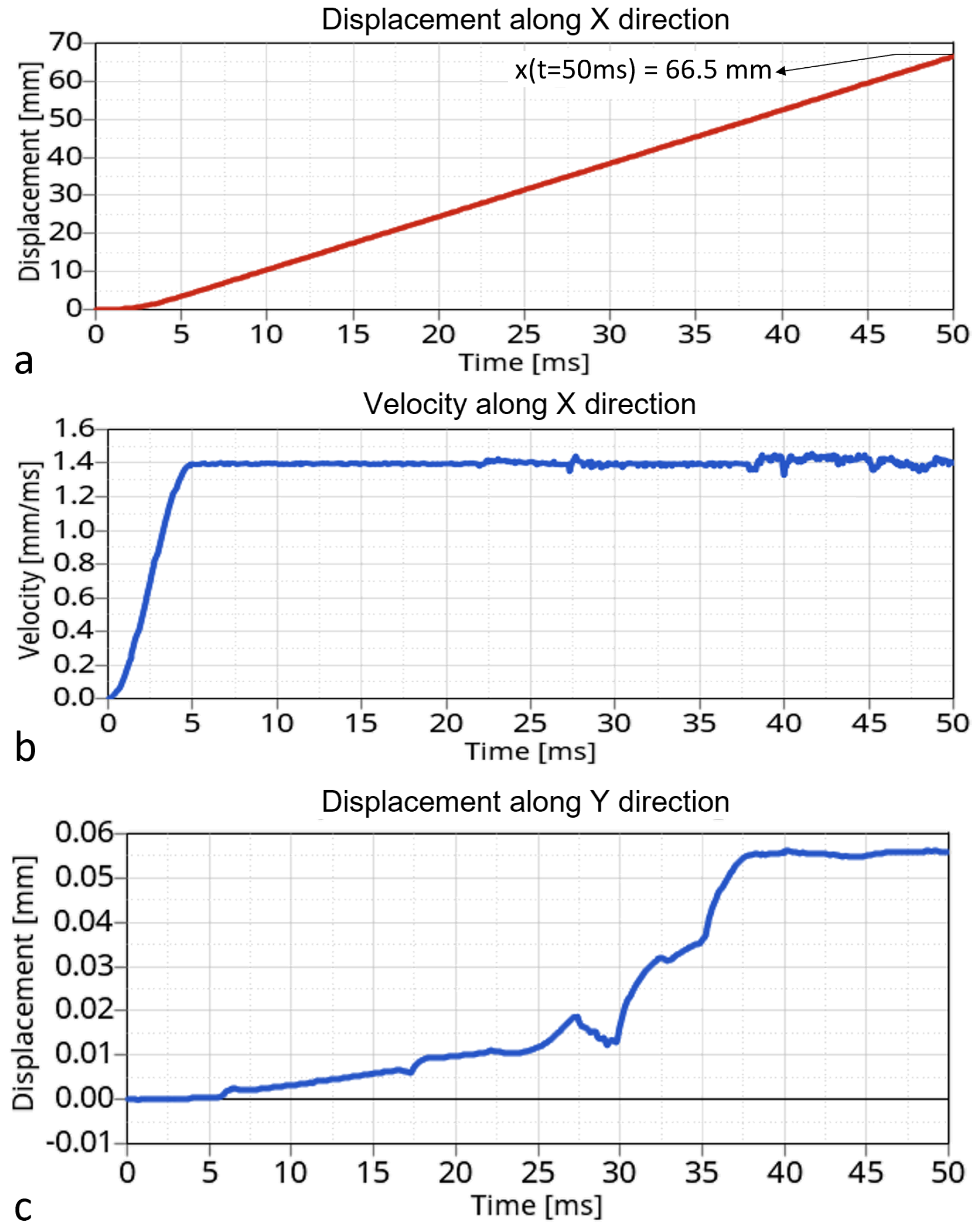
Figure 10 depicts the displacement and velocity related to a single rigid body, specifically the one that, at the beginning of the simulation, results in grip with the first pair of rollers on the first row. It should be noted that this set of quantities is representative of all other rigid bodies, as they share similar kinematics. When the analysis begins, the counter-rollers on the first row press the banknote against the motor-rollers, which begin to rotate. After 2 ms, the banknote starts to be dragged, and at the instant t = 50 ms, it will have traveled a full 66.5 mm. The speed of the banknote is 1400 mm/s, which is what one would expect having imposed this linear speed on the motor. If the banknote had been modeled using a single body, a pure motion along the X direction should be expected. In the present case, however, the banknote is decomposed in 200 boxes and, as a result, a slight slip along the Y axis is noticeable. The drifting of the banknote along the Y direction stops when the banknote comes into grip with the second row of rollers and counter-rollers, which stabilize the banknote. In fact, it can be seen how the position of the box along the Y direction remains constant from 38 ms onward.
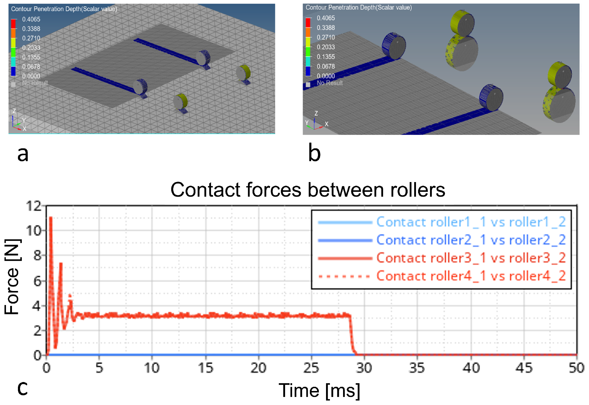
Figure 11 shows, on the left, two screenshots highlighting the contact state during the simulation. The blue ‘stripes’ on the banknote highlight where contact with the rollers occurred. The average penetration between the rollers and box is 0.04 mm. This means that the counter-roller interpenetrates the box on one side by 0.04 mm, and likewise, the roller on the opposite side, so that the overall interpenetration of the box is less than its thickness (0.1 mm). It is essential to comply with this condition; otherwise, the rollers would touch each other even when there is the banknote in grip. As for the pairs of rollers on the second row, the penetration value is higher (0.22 mm).
The total contact forces between the rollers, shown in the right portion of Figure 11, are different from zero only for the two pairs of rollers and counter-rollers on the second row because they do not have the banknote in their grip. Then, when the banknote reaches the second row, at about 30 ms, the corresponding rollers no longer exchange any contact forces.

4.2. Model with Four Motor-Rollers and Two Counter-Rollers

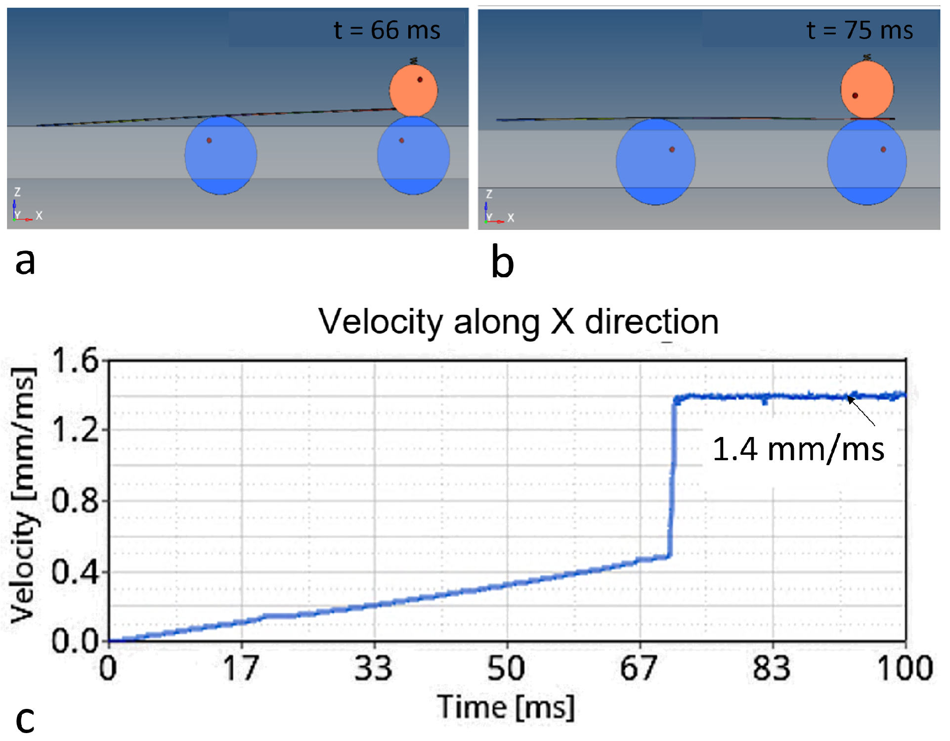
The second application concerns a MB model very similar to the previous one. The only difference is the lack of counter-rollers on the first row. Although this configuration is not realistic, i.e., counter-rollers are necessary to ensure proper banknote transportation, it helps verify the correct implementation of the contact between banknote and rollers. It is expected to observe a lower banknote dragging speed until the second row of rollers is reached. This is explained by the lower normal force pressing on the banknote at the beginning, resulting in a lower drag force, all other parameters being equal.
As shown in Figure 12, in this case, the banknote makes contact with some triangles of the support plane mesh. From the plot of the X-direction velocity of one of the rigid body boxes, it is evident that the banknote is transported very slowly until it comes into contact with the second row of rollers. In the full model, this occurred at the instant t = 30 ms (see Figure 11), in this case, however, it occurs after more than twice the time. The final speed that is achieved is always that resulting from the 1400 mm/s linear speed imposed to the motor rollers, as already shown in Figure 10.
In conclusion, it can be said that the banknote succeeds in being transported, despite the fact that there is no contribution from the first row of counter-rollers, and that, once it reaches the grip with the second row of rollers, it is not bounced back but continues its course correctly.

4.3. Model with Tilted Banknote

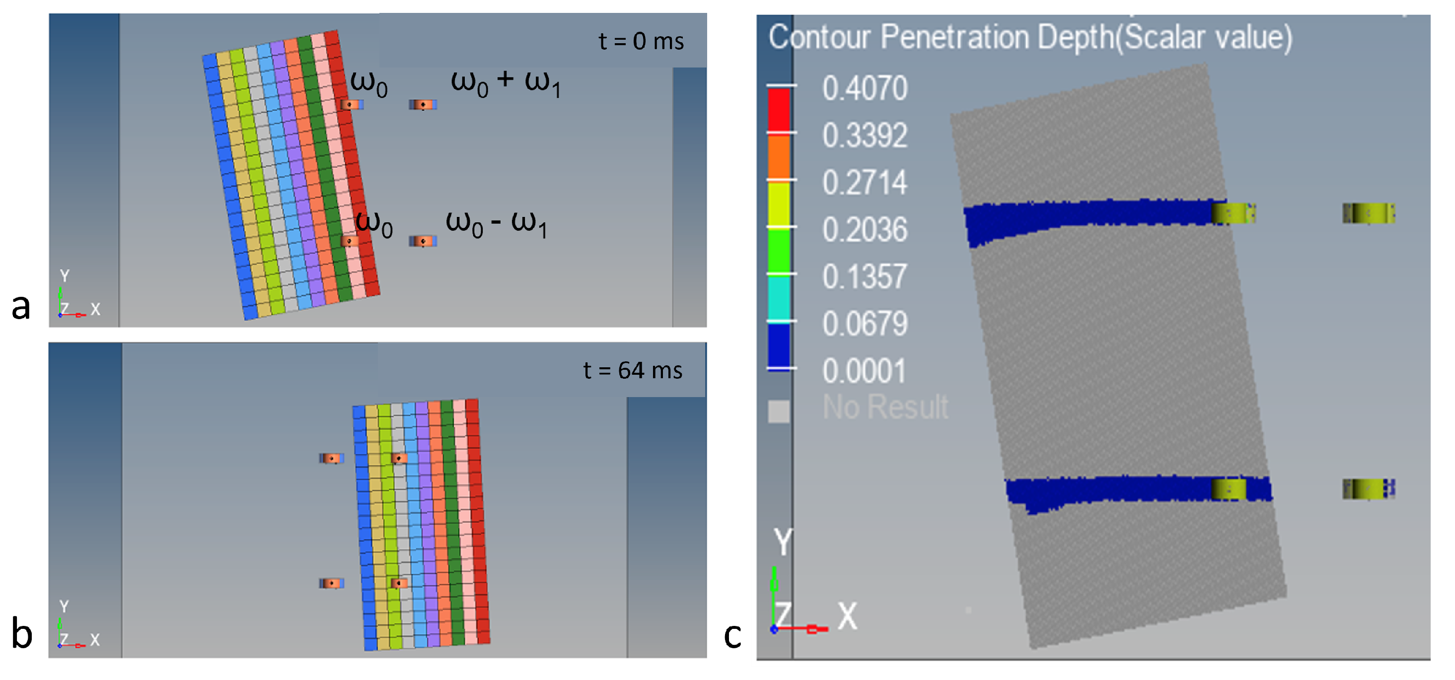
The third and final application involves the complete MB model, with the only difference being the inclination of the banknote. A rotation angle of 10 deg was imposed around the Z axis. Having developed the code to generate the points that make up the banknote with parameterized coordinates, the application of rigid rotation is very fast and simple. The goal is to verify the mechanism for correcting the tilt of the banknote by changing the rotation speeds of the rollers. Specifically, let us define ω 0 = 186 rad/s as the angular speed of the rollers under normal conditions. The speed of the first roller on the second row will be decreased by ω 1 = 50 rad/s, and we will increase the speed of the other motor-roller of the second row by the same amount. Four frames of the transport animation are shown in Figure 13. Initially, the banknote is tilted, and as it comes into grip with the second row of rollers, which have different speeds, it straightens.
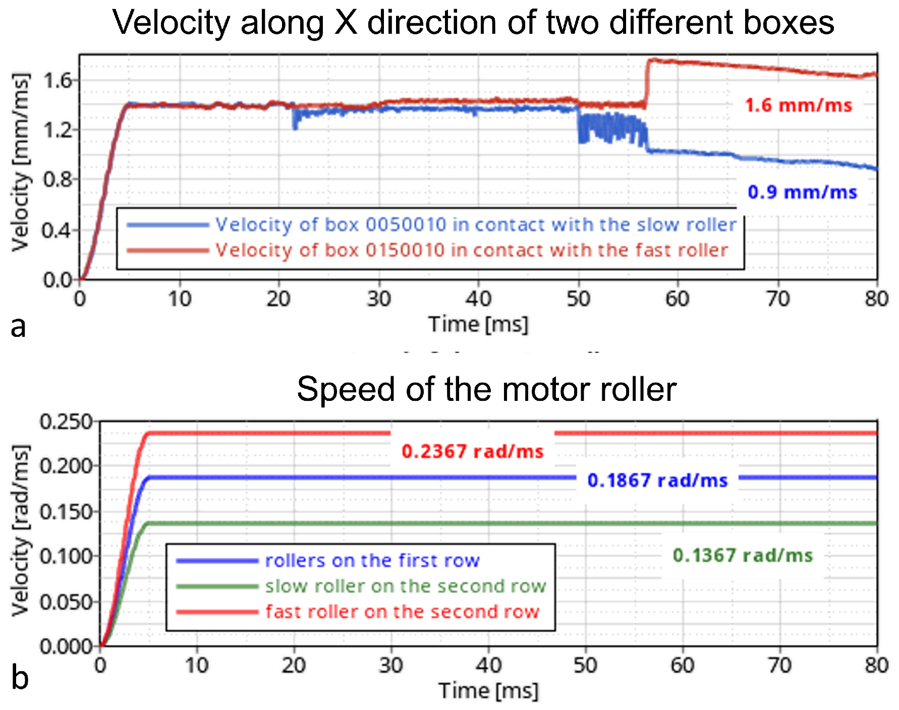
Figure 14 shows the depth of penetration on all bodies of the model. It can be seen that the two contact areas on the banknote are no longer parallel to the banknote’s short side. The right portion of Figure 14 focuses on the velocity of two boxes going into grip with different pairs of rollers and the velocity profiles of all four motor-rollers. It can be seen that the box in contact with the slow roller ( ω 0 ω 1 ) slows down to 0.9 mm/ms; meanwhile, box 0150010, in contact with the fast roller, speeds up to 1.6 mm/ms. The difference in banknote speed in the two different areas causes the correction of the angle of inclination.
It should be noted that the imposed ω 1 speed causes an over-correction of the angle. However, this is only a first effort aimed at evaluating the feasibility of the idea, and the calibration of the rollers’ speed is beyond the scope of the present work. In fact, this is a prime example of the potential of the present simulation tool. It enables the user to test new ideas to implement in the cash recycler without having to resort to costly and time-consuming experiments. In conclusion, the correction of the banknote’s tilt achieved through different speeds of the motor-rollers works, and it may be tested on the real machine after an optimization/calibration phase which may be conducted using the proposed simulation tool.
Before delving into the high-fidelity model of the cash recycler, the computational times of the present simplified model should also be discussed. A 50 ms simulation with a 0.01 ms time step takes about 4 min using a Intel(R) Xeon(R) CPU E5-1620 v4 @ 3.50 GHz Processor with 32 GB RAM and using four cores; it rises to about 25 min with a time step of one microsecond (h = 0.01 ms). These reduced computational times make the simplified model a perfect candidate to explore different design solutions quickly.

4.4. High-Fidelity Cash Recycler Model

In this section, the simulation of banknote transport through a high-fidelity model of a cash recycler is analysed. Although the whole transportation system has been simulated, this section will focus on a critical part of the cash recycler, i.e., the feeder group.
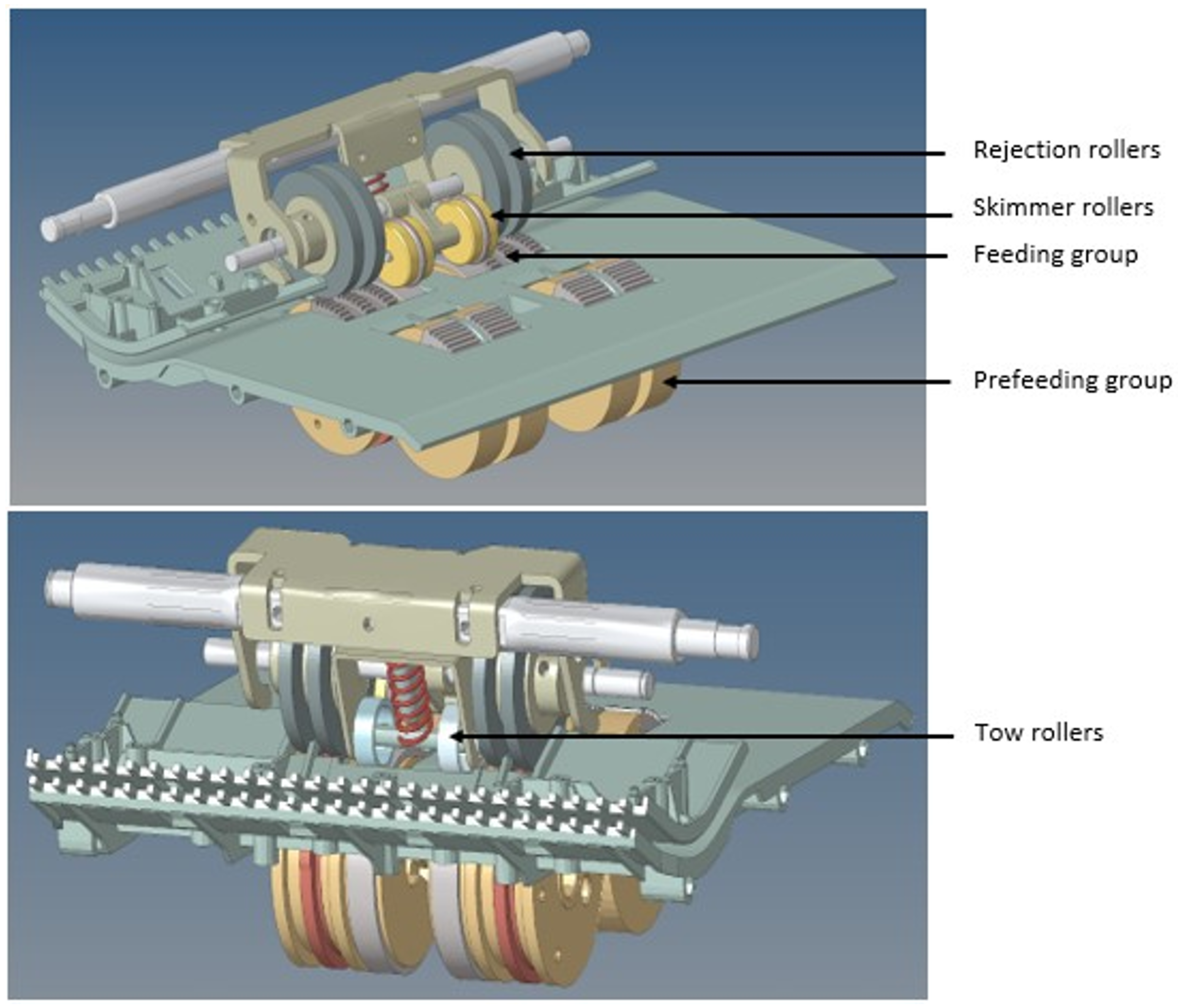
The purpose of the feeder is to convey the banknote past the rejection unit. The rejection unit is composed of the pulling system. The rejection rollers play the key role of allowing only one banknote at a time to pass. They are mounted with an interference of 0.2 mm with the feeding rollers, as visible in Figure 15.
In this context, it is critical to select the correct interference. If it were too large, the banknote would not be able to pass; if too small, more than one banknote would pass simultaneously. However, setting the right interference is not sufficient. It is also crucial to use the right materials so as to ensure a specific balance of friction. The friction between banknote and feeding rollers should be higher than that between banknote and rejection rollers. Furthermore, the friction between two overlapping banknotes should be less than that of the top banknote with the rejection rollers.
The purpose of the skimmer rollers is twofold, as follows:
  • They align the banknote by pivoting if it arrives tilted;
  • They press down on the banknote by providing the necessary drag force to get the banknote just below the rejection rollers but not past them (the feeding rollers are in charge of that).
The pulling system aims to advance the banknote quickly toward the exit. A spring with a preload of 15 N is used for this, so that the pulling force is increased. The rollers can rotate around the pulling axis, which can translate relative to the support on which it is mounted.
The MB model of the cash recycler was built on MotionView© by importing the CAD file. All the bodies are treated as rigid, so information on the material they are made of is not relevant to the bodies’ global deformations but rather to the contact parameters (contact stiffness and coefficient of friction). Motion, which in reality is transmitted by a motor to the pre-feeding and feeding rollers via a belt mechanism, is here imposed directly. Three different EUR 10 banknote models have been tested on the present cash recycler MB model as follows:
  • 200 boxes banknote model with center-to-center connections;
  • 200 boxes banknote model with edge-to-edge connections;
  • 600 boxes banknote model with edge-to-edge connections.
All investigated models manage to capture the macro-behavior of the banknote correctly. However, the first model, i.e., 200 boxes with center-to-center connections, shows some drawbacks. More specifically, as shown in Figure 16a, some boxes have angular positions radically different with respect to adjacent boxes. The cohesion between neighboring boxes is insufficient at some locations. This incorrect configuration may cause deviations of the banknote from the predetermined path and is, therefore, not deemed acceptable.
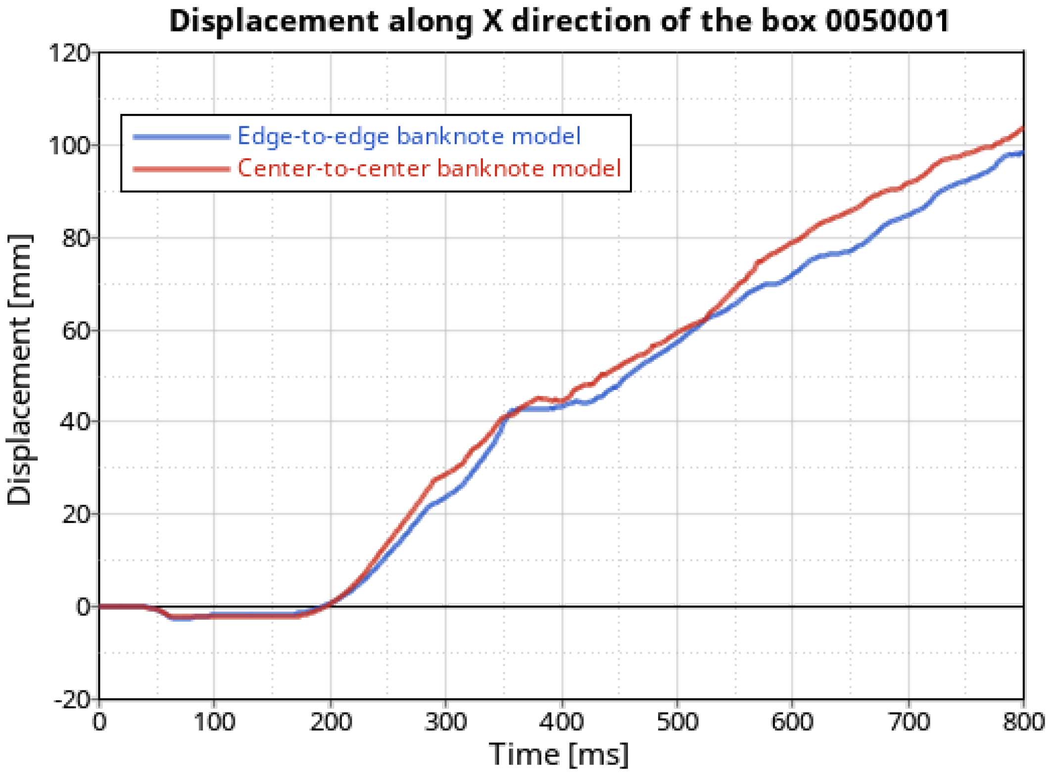
The problem is completely overcome when using the edge-to-edge banknote model, which ensures a sufficient level of cohesion between neighboring boxes. Furthermore, this second investigated model exhibits an additional advantage. During the simulation the banknote is supposed to remain in the same position when it is touching the rejection rollers but not yet in grip with the toothed rubber of the feeding rollers. This happens at around 400 ms from the start of the simulation.
Figure 17 shows the comparison between the displacement of one representative box coming from the two models, i.e., center-to-center vs. edge-to-edge. It can be seen that the curve representing the edge-to-edge model remains horizontal at 400 ms, while the one representing the center-to-center model does show some unrealistic advancement.
The third and final model sees edge-to-edge connections, which proved to be the most effective, and a finer discretization. In the present case, the number of boxes has been tripled, to ensure significantly smaller boxes, especially in the Y-direction. Indeed, the critical part of transport in this system is the transition between the rejection rolls and the feeding rollers, where the gap the banknote has to pass through is at its minimum. While using a 200 box model, some interpenetration between boxes and rollers was visible at this critical step, Figure 16b shows that, when using a finer discretization, boxes are arranged according to the available spaces between the rejection rollers and the feeding rollers. This higher precision does come at a higher computational cost; in fact, the simulation time increases by one order of magnitude when multiplying the number of boxes by a factor of 3 (7 h vs. 3 days). This is mainly due to the contact algorithm having to handle an increased number of entities at the same time. Some strategies to limit the computational time are possible, e.g., finer box discretization only in some critical areas or highly efficient time integration algorithms [28,29]. However, the authors recommend the use of the simplified model during the design phase, while leaving the high-fidelity version for the validation/certification phase of the project.

5. Conclusions

The methodology developed uses a MB approach to simulate banknote transport. The banknote is modeled with a set of rigid bodies, represented by boxes (parallelepipeds), connected at the corners with springs. The springs have the function of giving flexibility to the whole system, and both linear and nonlinear characteristics can be assigned. The reasons which make this method original and the best choice when having to create a MB model of a paper sheet are outlined as follows:
  • Greater simplicity in defining the contact. The contact between deformable surfaces is prone to convergence problems, especially when considering large displacements typical of transportation. Modeling the banknote as a ‘grid’ of rigid bodies allows the use of a more robust contact definition. This feature not only ensures convergence but significantly reduces computational times;
  • Possibility of using the nonlinear curves characteristic of the orthotropic paper material;
  • Lack of cumbersome pre-processing steps typical of dynamic condensation. In the present case, a Python code automatically creates the banknote starting from a simple set of user-defined parameters;
  • Complete control and customization of the banknote system, as one can vary quantities such as thickness, friction coefficients, etc., in specific areas.
The proposed simulation methodology has been validated both on simplified and on high-fidelity models of a cash recycler handling a EUR 10 banknote. In light of the results obtained, the model of the banknote decomposed into rigid bodies can be considered effective in modeling banknote transport.
Transport under different conditions (standard, reduced drag-force, tilt correction of the banknote, and contact with different materials) was simulated, and the response of the banknote was satisfactory. This includes the complex ‘feeder’ system simulated in the high-fidelity model, where the banknote advances past the rejection rollers only when in grip with the rubber teeth of the peeling rollers and not when in contact with the plastic, whose coefficient of friction is lower with respect to the rubber part.
The analysis of the results allowed the model of the banknote to be refined. It was shown that the center-to-center connection of the boxes is too loose, and the edge-to-edge connection should be preferred instead.
Finally, the importance of the boxes dimension was highlighted. Using boxes that are too large compared to the space the banknote has to pass through, results in too much interpenetration between the contacting bodies.
However, the limitations to this study should be acknowledged. While the rigid-body decomposition approach ensures robustness and computational efficiency, it introduces approximations that may not fully capture the complex deformations of highly flexible banknotes, especially under extreme conditions. Additionally, the model’s accuracy depends on properly calibrated material properties and contact parameters, which may require experimental validation for specific cases. Future work could focus on refining the model to better account for localized deformations and exploring more advanced material models while maintaining computational efficiency. Additionally, a possible expansion of the present model may be directed to non-flat configurations, i.e., bent banknotes, which can be modeled by modifying the relative position of the rigid bodies that compose the banknote and by tuning (increasing) the values of the springs in distinct directions, through a specific tuning procedure.
In conclusion, the presented banknote and contact model is effective in simulating banknote transport in a MB system, and can be a tool for testing different construction solutions for the banknote transport mechanism. It is possible to change both the characteristics of the paper and those of other system components, such as adding rollers of different shapes and materials, and see how the banknote behaves overall. In this way, unsuccessful solutions can be discarded a priori, without having to build any physical prototype. Furthermore, the present model is fit to be adapted to any other application which involves paper sheets being transported and handled.

Author Contributions

Conceptualization, L.G., C.G., C.D., S.L. and D.E.; methodology, L.G., C.G., C.D., S.L. and D.E.; software, S.L. and D.E.; validation, L.G., C.G. and D.E.; writing—original draft preparation, C.G.; writing—review and editing, L.G. and C.G.; supervision, C.D. and S.L. All authors have read and agreed to the published version of the manuscript.

Funding

This research received no external funding.

Institutional Review Board Statement

Not applicable.

Informed Consent Statement

Not applicable.

Data Availability Statement

The raw data supporting the conclusions of this article will be made available by the authors on request.

Conflicts of Interest

Author Samuele Libetti and Davide Eleuteri were employed by the company Sesami. The remaining authors declare that the research was conducted in the absence of any commercial or financial relationships that could be construed as a potential conflict of interest.

Abbreviations

The following abbreviations are used in this manuscript:
MBMultibody
LFLinear flexible
NLFENon linear finite element
FEFinite element
CADComputer-aided drawing

References

  1. Tedder, K.; Huber, R. 2020 Health of Cash Study. 2020. Available online: https://javelinstrategy.com/research/2020-health-cash-study (accessed on 17 October 2022).
  2. Halpin, J. The Future of Retail Cash Technology; Technical Report, ACMA Currency Notes; ACMA: Melbourne, Australia, 2020. [Google Scholar]
  3. Bruna, A.; Farinella, G.; Guarnera, G.; Battiato, S. Forgery Detection and Value Identification of Euro Banknotes. Sensors 2013, 13, 2515–2529. [Google Scholar] [CrossRef] [PubMed]
  4. Simon, J.W. A Review of Recent Trends and Challenges in Computational Modeling of Paper and Paperboard at Different Scales. Arch. Comput. Methods Eng. 2021, 28, 2409–2428. [Google Scholar] [CrossRef]
  5. Sanjon, C.W.; Leng, Y.; Hauptmann, M.; Groche, P.; Majschak, J.P. Methods for Characterization and Continuum Modeling of Inhomogeneous Properties of Paper and Paperboard Materials: A Review. BioResources 2024, 19, 6804–6837. [Google Scholar] [CrossRef]
  6. Garbowski, T.; Gajewski, T.; Grabski, J.K. Estimation of the Compressive Strength of Corrugated Cardboard Boxes with Various Perforations. Energies 2021, 14, 1095. [Google Scholar] [CrossRef]
  7. Marin, G.; Srinivasa, P.; Nygårds, M.; Östlund, S. Experimental and Finite Element Simulated Box Compression Tests on Paperboard Packages at Different Moisture Levels. Packag. Technol. Sci. 2021, 34, 229–243. [Google Scholar] [CrossRef]
  8. Aduke, R.N.; Venter, M.P.; Coetzee, C.J. Numerical Modelling of Corrugated Paperboard Boxes. Math. Comput. Appl. 2024, 29, 70. [Google Scholar] [CrossRef]
  9. Sugiyama, H.; Kobayashi, N. Analysis of Spaghetti Problem Using Multibody Dynamics. Trans. Jpn. Soc. Mech. Eng. Ser. C 1999, 65, 910–915. [Google Scholar] [CrossRef]
  10. Shabana, A.A. Flexible Multibody Dynamics: Review of Past and Recent Developments. Multibody Syst. Dyn. 1997, 1, 189–222. [Google Scholar] [CrossRef]
  11. Bauchau, O.A. Flexible Multibody Dynamics; Springer: Berlin/Heidelberg, Germany, 2010. [Google Scholar]
  12. Simeon, B. Computational Flexible Multibody Dynamics; Springer: Berlin/Heidelberg, Germany, 2013. [Google Scholar]
  13. Li, Y.; Stapleton, S.E.; Reese, S.; Simon, J.W. Anisotropic elastic-plastic deformation of paper: In-plane model. Int. J. Solids Struct. 2016, 100–101, 286–296. [Google Scholar] [CrossRef]
  14. Skrinjar, L.; Slavič, J.; Boltežar, M. A review of continuous contact-force models in multibody dynamics. Int. J. Mech. Sci. 2018, 145, 171–187. [Google Scholar] [CrossRef]
  15. Hurty, W.C. Dynamic analysis of structural systems using component modes. AIAA J. 1965, 3, 678–685. [Google Scholar] [CrossRef]
  16. Craig, R.R.; Bampton, M.C.C. Coupling of substructures for dynamic analyses. AIAA J. 1968, 6, 1313–1319. [Google Scholar] [CrossRef]
  17. MacNeal, R.H. A hybrid method of component mode synthesis. Comput. Struct. 1971, 1, 581–601. [Google Scholar] [CrossRef]
  18. Rubin, S. Improved Component-Mode Representation for Structural Dynamic Analysis. AIAA J. 1975, 13, 995–1006. [Google Scholar] [CrossRef]
  19. R. Craig, J. On the use of attachment modes in substructure coupling for dynamic analysis. In Proceedings of the AIAA/ASME 18th Structural Dynamics and Materials Conference, San Diego, CA, USA, 21–23 March 1977. [Google Scholar] [CrossRef]
  20. O’Shea, J.J.; Jayakumar, P.; Mechergui, D.; Shabana, A.A.; Wang, L. Reference Conditions and Substructuring Techniques in Flexible Multibody System Dynamics. J. Comput. Nonlinear Dyn. 2018, 13, 041007. [Google Scholar] [CrossRef]
  21. Mitra, M.; Zucca, S.; Epureanu, B.I. Adaptive Microslip Projection for Reduction of Frictional and Contact Nonlinearities in Shrouded Blisks. J. Comput. Nonlinear Dyn. 2016, 11, 041016. [Google Scholar] [CrossRef]
  22. Gastaldi, C.; Zucca, S.; Epureanu, B.I. Jacobian projection reduced-order models for dynamic systems with contact nonlinearities. Mech. Syst. Signal Process. 2018, 100, 550–569. [Google Scholar] [CrossRef]
  23. Sun, H.; Zhang, D.; Wu, Y.; Shen, Q.; Hu, D. A Semi-Analytical Multi-Harmonic Balance Method on Full-3D Contact Model for Dynamic Analysis of Dry Friction Systems. Chin. J. Aeronaut. 2024, 37, 309–329. [Google Scholar] [CrossRef]
  24. MotionSolve Reference Guide 2023. Available online: https://2023.help.altair.com/2023.1/hwsolvers/ms/topics/chapter_heads/msolve_ref_guide_r.htm (accessed on 5 January 2025).
  25. Learn Multi-Body Simulation with Altair MotionSolve. Available online: https://advanced-eng.cz/wp-content/uploads/2021/06/2021_eBook_Learn_Multi_Body_Simulation_with-Altair_Motion_Solve.pdf (accessed on 5 January 2025).
  26. Lagier, F.; Massicotte, B.; Charron, J.P. 3D Nonlinear Finite-Element Modeling of Lap Splices in UHPFRC. J. Struct. Eng. 2016, 142, 04016087. [Google Scholar] [CrossRef]
  27. Peter, B.; Sänger, N. A Nonlinear Finite Element Framework for Flexible Multibody Dynamics: Rotationless Formulation and Energy-Momentum Conserving Discretization. In Multibody Dynamics; Springer: Dordrecht, The Netherlands, 2009; pp. 119–141. [Google Scholar] [CrossRef]
  28. Gastaldi, C.; Berruti, T.M. Competitive Time Marching Solution Methods for Systems with Friction-Induced Nonlinearities. Appl. Sci. 2018, 8, 291. [Google Scholar] [CrossRef]
  29. Marques, F.; Flores, P.; Claro, J.C.P.; Lankarani, H.M. Modeling and analysis of friction including rolling effects in multibody dynamics: A review. Multibody Syst. Dyn. 2018, 45, 223–244. [Google Scholar] [CrossRef]
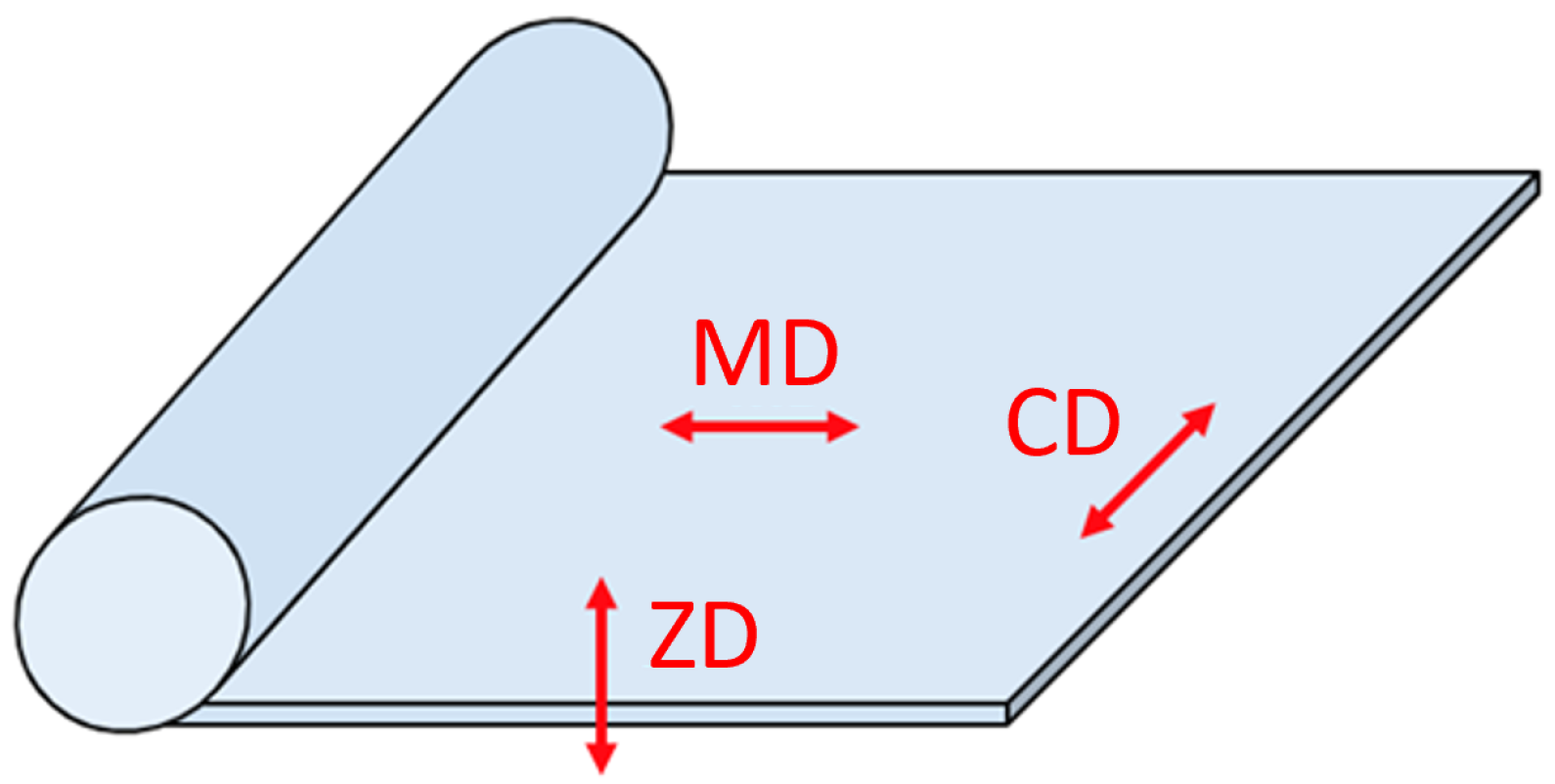
Figure 1. Principal directions of paper banknote.
Applsci 15 02283 g001
Figure 2. Example of contact defined using ‘Point on deformable surface’, typical of the sub-structuring technique.
Applsci 15 02283 g002
Figure 3. Discretization of the banknote into rigid bodies with edge-to-edge connections.
Applsci 15 02283 g003
Figure 4. Center-to-center connection to represent the banknote focus on translational springs (left) and edge-to-edge connection focus on rotational springs (right).
Applsci 15 02283 g004
Figure 5. EUR 10 banknote discretized into 200 boxes.
Applsci 15 02283 g005
Figure 6. Experimental set-up of banknote bending measurement while keeping the short side fixed (a). Experiment reproduction in MotionView© (b). Contour diagram of the deformable surface (c). Displacement along the Z direction of point P on the short free side (d).
Applsci 15 02283 g006
Figure 7. Example of mesh-based contact between box and cylinder.
Applsci 15 02283 g007
Figure 8. Representative scheme of the simplified MB model.
Applsci 15 02283 g008
Figure 9. Screenshots at time instants t = 0, t = 18, t = 30, and t = 50 ms of 50 ms simulations representing the banknote being transported by 4 motor-rollers and 4 counter-rollers. General view (a). View on the XZ plane (b).
Applsci 15 02283 g009
Figure 10. Kinematic quantities related to one of the rigid body boxes used to discretize the banknote as functions of time. (a) Displacement along X direction. (b) Velocity along X direction. (c) Displacement along Y direction.
Applsci 15 02283 g010
Figure 11. Contact force between rollers (a). Screenshots showing the contact penetration during simulation (b,c).
Applsci 15 02283 g011
Figure 12. Screenshots showing the banknote being transported by 4 motor rollers and 2 counter-rollers (a,b). Velocity of one of the rigid body boxes along X direction (c).
Applsci 15 02283 g012
Figure 13. Frames showing the tilted banknote being transported and rotated by 4 pairs of motor- and counter-rollers (a,b). Contact penetration during transport of tilted banknote (c).
Applsci 15 02283 g013
Figure 14. Velocity along X direction of two different boxes in contact with different rollers (a). Speed of the different rollers (b).
Applsci 15 02283 g014
Figure 15. High-fidelity model of the cash recycler. Focus on the feeder and the rejection unit.
Applsci 15 02283 g015
Figure 16. Frames showing the incorrect configuration of the center-to-center banknote model (a), and the correct configuration of the edge-to-edge banknote model (b).
Applsci 15 02283 g016
Figure 17. Displacement along the X coordinate of one representative box of the banknote model; comparison between the center-to-center and edge-to-edge banknote models.
Applsci 15 02283 g017
Table 1. Relevant quantities of banknote model.
ParameterSymbolValue
Banknote mass (g)M0.72
Banknote length short side (mm) L x 67
Banknote length long side (mm) L y 127
Banknote thickness (mm)s0.1
Number of boxes along X n x 10
Number of boxes along Y n y 20
Box length along X d x 7.44
Box length along Y d y 6.68
Box mass (g)m0.0036
Table 2. Summary table of stiffness and damping values of the bushing entity in the center-to-center and edge-to-edge configurations.
Center-to-Center Connection
Translational stiffness (N/mm)Translational damping (N/mm/ms) ξ
k x 317 c x 0.260.12
k y 124 c x 0.160.12
Rotational stiffness (N mm/rad)Rotational damping (N mm ms/rad) ξ
k t x 0.27 c t x 7.480.12
k t y 0.45 c t y 3.220.04
k t z 10 c t z 45.50.12
Edge-to-Edge Connection
Translational stiffness (N/mm)Translational damping (N/mm/ms) ξ
k x 158 c x 0.130.12
k y 62 c x 0.080.12
Rotational stiffness (N mm/rad)Rotational damping (N mm ms/rad) ξ
k t x 0.15 c t x 5.580.12
k t y 0.185 c t y 2.060.04
k t z 5 c t z 230.12
Table 3. Summary table of the components of the simplified MB model.
DescriptionMass (g)Dimensions (mm)
Support plane681227 × 300 × 10
Motor-rollers0.88Diameter = 15 Thickness = 5
Counter-rollers0.39Diameter = 10 Thickness = 5
Table 4. Summary table of contact parameters.
ParameterRollers/
Counter-Rollers
Plane/BanknoteRollers/BanknoteCounter-Rollers/
Banknote
Stiffness k (N/ m m 3 / 2 )30.5100300300
Restitution coeff. C R 0.50.50.50.5
Friction coeff. μ 10.310.33
Disclaimer/Publisher’s Note: The statements, opinions and data contained in all publications are solely those of the individual author(s) and contributor(s) and not of MDPI and/or the editor(s). MDPI and/or the editor(s) disclaim responsibility for any injury to people or property resulting from any ideas, methods, instructions or products referred to in the content.