Discrete Multi-Objective Grey Wolf Algorithm Applied to Dynamic Distributed Flexible Job Shop Scheduling Problem with Variable Processing Times

Abstract

Uncertainty in processing times is a key issue in distributed production; it severely affects scheduling accuracy. In this study, we investigate a dynamic distributed flexible job shop scheduling problem with variable processing times (DDFJSP-VPT), in which the processing time follows a normal distribution. First, the mathematical model is established by simultaneously considering the makespan, tardiness, and total factory load. Second, a chance-constrained approach is employed to predict uncertain processing times to generate a robust initial schedule. Then, a heuristic scheduling method which involves a left-shift strategy, an insertion-based local adjustment strategy, and a DMOGWO-based global rescheduling strategy is developed to dynamically adjust the scheduling plan in response to the context of uncertainty. Moreover, a hybrid initialization scheme, discrete crossover, and mutation operations are designed to generate a high-quality initial population and update the wolf pack, enabling GWO to effectively solve the distributed flexible job shop scheduling problem. Based on the parameter sensitivity study and a comparison with four algorithms, the algorithm’s stability and effectiveness in both static and dynamic environments are demonstrated. Finally, the experimental results show that our method can achieve much better performance than other rules-based reactive scheduling methods and the hybrid-shift strategy. The utility of the prediction strategy is also validated.

1. Introduction

The flexible job shop scheduling problem (FJSP) aims to address the challenges of determining the processing sequence and machine allocation for operations within production systems [1]. It has been proven to be a complex combinatorial optimization problem [2]. Moreover, manufacturing enterprises often have multiple factories, each of which can be considered a flexible job shop [3]. As a result, it is essential to consider the allocation of jobs across these factories, which is the so-called distributed flexible job shop scheduling problem (DFJSP). The DFJSP is an extension of the classical FJSP, and it is characterized by its enhanced applicability to real-world production environments [4]. Specifically, it addresses substantial challenges regarding the management of distributed resources and coordination across factories. The development of efficient algorithms for the DFJSP is a critical topic in both academic and engineering research.

In real production environments, processing times are often uncertain due to factors such as process damage, the equipment status, and operator proficiency [5]. These dynamic events can directly disrupt the original scheduling plan, necessitating real-time adjustments to job sequencing and resource allocation. As a result, the traditional DFJSP model needs to be extended to a dynamic DFJSP with variable processing time (DDFJSP-VPT) to address the impact of processing time variability, as a dynamic event, on scheduling decisions. In the DDFJSP-VPT, the scheduling problem requires not only the design of an efficient solution in the initial stage but also the ability to adapt to the deviations from estimated times. It is important to adjust the scheduling strategy in real time to maintain the system’s performance and stability. This imposes higher requirements on scheduling algorithms, demanding both robustness and flexibility to respond to such dynamic fluctuations [6].

The methods for solving the DFJSP can be mainly divided into exact algorithms, heuristic algorithms, and metaheuristic algorithms. The exact methods are not able to find feasible solutions for comparatively complex models in acceptable timeframes. Moreover, although heuristic algorithms are easy to implement, it is difficult to obtain high-quality solutions. In contrast, metaheuristic algorithms have been widely used since they can maintain a balance between the solution quality and operational efficiency. As a relatively new member of this group of methods, the grey wolf algorithm (GWO) is inspired by the social hierarchy and predatory behavior of grey wolves; it has the advantages of simplicity, flexibility, and ease of implementation. So far, GWOs have been applied to a variety of scheduling problems, such as the job shop scheduling problem [7], the flexible job shop scheduling problem [8,9,10], the flow job shop scheduling problem [11], and the distributed flexible job shop scheduling problem [12,13]. However, to the best of our knowledge, there is no reported work about using the GWO to solve the DDFJSP-VPT.

Few existing studies have fully considered the effects of variable processing times on the DFJSP since they assume that the processing time is predetermined and unchangeable, overlooking the potential for dynamic changes during practical production. Moreover, the existing scheduling methods struggle to address this issue, quickly respond to similar events, and make reasonable decisions. Thus, it remains essential to model and examine the changes in the processing time of the DFJSP.

To address the above challenges, this paper introduces a novel approach that focuses on handling dynamic changes in processing times within the framework of the DDFJSP-VPT. Specifically, we make the following contributions:

(1)

A multi-objective DDFJSP-VPT mathematical model is established with the objectives of simultaneously minimizing the makespan, total factory load, and tardiness, in which the processing time fluctuation follows a normal distribution.

(2)

Based on the chance-constrained programming theory, the actual processing times are predicted utilizing the quantiles of the given normal distribution and the permissible violation degree of the constraints. This approach enhances the robustness of the obtained initial scheduling solution, reducing the impact of dynamic events on the original schedule.

(3)

We propose a heuristic scheduling method to solve the associated model. Using this method, a left-shift adjustment strategy, an insertion-based local adjustment strategy, and a global adjustment strategy based on a discrete multi-objective grey wolf algorithm (DMOGWO) are developed.

(4)

An initialization strategy that combines multiple heuristic rules is designed to generate the initial populations with certain levels of quality and diversity. Additionally, discrete crossover and mutation operators are used for position updates in the wolf pack, enabling the GWO to adaptively resolve the scheduling problem.

(5)

To evaluate the effectiveness of the proposed methods, a series of experiments are conducted with four main purposes: (i) conducting a sensitivity analysis of the population size in DMOGWO to investigate its impact on the algorithm’s performance; (ii) comparing the performance of DMOGWO with other representative algorithms on solving a static DFJSP and DDFJSP-VPT to assess its competitiveness in terms of both static and dynamic scenarios; (iii) evaluating the performance of the proposed scheduling method against other dynamic scheduling methods with regard to dynamic environments; and (iv) analyzing the impact of the prediction scheme on scheduling efficiency and robustness.

The structure of the study is as follows: Section 2 presents a review of the literature on dynamic DFJSPs and FJSPs with variable processing times. The problem description and mathematical model are presented in Section 3. Section 4 and Section 5 detail the processing time prediction methods and the proposed scheduling method, respectively. Experimental results are discussed in Section 6. Finally, Section 7 concludes the paper and outlines potential directions for future research.

2. Literature Review

2.1. Dynamic Distributed Flexible Job Shop Scheduling Problems

The dynamic flexible job shop scheduling problem has attracted considerable attention due to its ability to effectively address dynamic events in manufacturing environments, such as machine failures, new job arrivals, and emergency order insertions. However, as manufacturing systems evolve towards distributed and multi-workshop collaborative models, the scheduling optimization methods for single-workshop systems have increasingly shown limitations when dealing with complex dynamic environments and resource distribution issues. In this context, the dynamic DFJSP has emerged as a new research direction in the field of production scheduling, drawing the attention of the academic community. Although research on the dynamic DFJSP is still in its early stages, a few studies have focused on multi-workshop collaborative scheduling and dynamic event handling. Gong et al. [14] studied the operation inspection problem to prevent defective products from being passed to the next manufacturing stage. In their paper, a hybrid rescheduling method that combines event-driven rescheduling and complete rescheduling was designed. Gong et al. [15] further introduced an effective reformative memetic algorithm to solve the DFJSP with order cancellation, in which jobs with different processing states are handled in various ways. Zhang et al. [16] presented an improved memetic algorithm to solve the energy-efficient DFJSP considering machine failures. In order to resolve the dynamic low-carbon distributed scheduling problem, considering new job arrivals and job transfers, Chen et al. [17] proposed a real-time scheduling method combining deep reinforcement learning with the Rainbow Deep-Q network. Wang et al. [18] proposed a real-time scheduling method based on evolutionary game theory to optimize the makespan, energy consumption, and critical machine workload.

However, all the above-mentioned studies assume that the processing times are deterministic, and they overlook the variability that may occur in processing times due to various uncertain factors during production. This variability can significantly impact scheduling decisions, highlighting the need for in-depth research into variable processing times.

2.2. Flexible Job Shop Scheduling Problems with Variable Processing Time

The representative method for solving the FJSP with variable processing time (FJSP-VPT) mainly focused on generating a robust initial scheduling scheme. Lin et al. [19] studied the stochastic FJSP with processing times following normal and gamma prior distributions, using a Monte Carlo simulation to address the uncertainty in processing times. Jin et al. [20] introduced neutrosophic sets to model uncertain processing times in the FJSP with path flexibility. Furthermore, an improved teaching–learning-based optimization algorithm was proposed to solve the corresponding problem. Caldeira and Gnanavelbabu [21] introduced a hybrid approach combining Monte Carlo simulations with the Jaya algorithm to solve the FJSP-VPT. Sun et al. [22] proposed a hybrid co-evolutionary algorithm based on the Markov random field decomposition strategy for the FJSP with stochastic processing times, with the aim of minimizing both the expected value and the variance of the makespan. Mokhtari and Dadgar [23] proposed a simulation–optimization framework based on a simulated annealing optimizer and Monte Carlo simulator to handle the FJSP with variable processing times and machine failures. Very recently, some rescheduling-based solution methods have been presented. Shahgholi Zadeh et al. [24] generated an original scheduling plan based on theoretical processing times and performed dynamic rescheduling in response to the variation in processing time in the subsequent actual processing stage. Zhong et al. [25] also addressed the dynamic FJSP-VPT by developing a scheduling model based on a chance-constrained approach, which transforms the uncertainty problem into a deterministic problem. The scheduling solution was then obtained using operation shifting and rescheduling strategies. Zhang et al. [26] also investigated the dynamic FJSP-VPT, proposing a solution approach that integrates Markov decision processes with reinforcement learning methods.

These above studies focus on single-shop production environments. Nevertheless, research related to distributed production scheduling is considerably limited. Fu et al. [27] solved the DFJSP with variable processing times by proposing a stochastic programming model combined with stochastic simulation and an evolutionary algorithm to minimize the makespan and total tardiness. In a distributed environment, multiple workshops can effectively mitigate the impact of variants in processing in individual shops through dynamic resource allocation and collaboration, reducing the overall scheduling disruption. Therefore, it is highly important to study the variable processing time problem in distributed environments.

3. Formulation of Multi-Criteria Optimization Problem

3.1. Problem Description

The DDFJSP-VPT can be described as follows: a set of n jobs $J$ = $\left\{J_1,J_2,\dots ,J_n\right\}$ must be processed in $w$ flexible job-shop-type factories $\left\{U_1,U_2,\dots ,U_w\right\}$. Each job $J_i$ consists of one or more operations $\left\{O_{i1},O_{i2},\dots ,O_{i{n}_i}\right\}$, and each factory $U_l$ has $m_l$ machines $\left\{M_{l1},M_{l2},\dots ,M_{lm}\right\}$. Once a job is assigned to a designated factory, all of its operations must be processed in it, and each operation can be assigned to one or more machines in this factory. When operation $O_{ij}$ is assigned to machine $M_{lk}$ in factory $U_l$, its theoretical processing time is $p_{ij}^{lk}$. However, due to various uncertainties in real-world production, the actual processing time of each operation is subject to fluctuations and is denoted as ${\tilde{p}}_{ij}^{lk}$. The scheduling consists of three subproblems: the factory assignment of jobs, machine selection for operations, and the sequencing of operations in an uncertain environment arising from changes in processing times. The objective is to optimize the performance of the scheduling system while ensuring all constraints are satisfied.

As is the case in much of the existing literature, the following assumptions are made: (1) all machines are available and all jobs can begin processing from the initial moment. (2) Each factory has the capacity to process all jobs. (3) Each machine can process at most one operation at a time. (4) All operations of the same job must be processed within the same factory. (5) Each operation can be processed by only one machine. (6) Once a job begins processing, it cannot be interrupted. (7) The transport time, setup time, and release time are not considered. (8) Only the processing phase of jobs is considered. Disassembly and assembly phases are not included.

3.2. Mathematical Modeling for the DDFJSP-VPT

Some notations used to describe the mathematical model are listed in

Table 1. Notations used to describe the mathematical model.

Notation	Description
Parameters:
$n$	Number of jobs
$J_i$	The ith job
$n_i$	$\mathrm{Number} \mathrm{of} \mathrm{operations} \mathrm{in} \mathrm{job} J_i$
w	Number of factories
$U_l$	The lth factory
$m_l$	$\mathrm{Number} \mathrm{of} \mathrm{machines} \mathrm{in} \mathrm{factory} U_l$
$O_{ij}$	$\mathrm{The} j\mathrm{th} \mathrm{operation} \mathrm{in} \mathrm{job} J_i$
$M_{lk}$	$\mathrm{The} k\mathrm{th} \mathrm{machine} \mathrm{in} \mathrm{factory} U_l$
${\mathsf{\Omega }}_{ij}^l$	$\mathrm{Set} \mathrm{of} \mathrm{machines} \mathrm{in} U_l \mathrm{that} \mathrm{can} \mathrm{process} O_{ij}$
$p_{ij}^{lk}$	$\mathrm{Theoretical} \mathrm{processing} \mathrm{time} \mathrm{of} \mathrm{operation} O_{ij} \mathrm{on} \mathrm{machine} M_{lk}$
${\tilde{p}}_{ij}^{lk}$	$\mathrm{Actual} \mathrm{processing} \mathrm{time} \mathrm{of} O_{ij} \mathrm{on} m_{lk}, \mathrm{a} \mathrm{random} \mathrm{variable} \mathrm{with} {\tilde{p}}_{ij}^{lk}~N({\mu }_{ij}^{lk},{\sigma }_{ij}^{lk})$
${\delta }_i$	$\mathrm{Set} \mathrm{of} \mathrm{processable} \mathrm{factories} \mathrm{for} J_i$
$D{D}_i$	$\mathrm{Due} \mathrm{date} \mathrm{of} J_i$
L	A sufficiently large constant
Decision Variables:
$t_l$	$\mathrm{Implementation} \mathrm{time} \mathrm{point} \mathrm{of} \mathrm{the} \mathrm{adjustment} \mathrm{strategy}, l=1,2,\dots$
$x_{ij}^{lk}$	$\mathrm{If} \mathrm{operation} O_{ij} \mathrm{is} \mathrm{processed} \mathrm{on} M_{lk}, \mathrm{then} x_{ij}^{lk}=1, \mathrm{else} x_{ij}^{lk}=0$
$y_{ij}^{lkr}$	$\mathrm{If} O_{ij} \mathrm{is} \mathrm{the} r\mathrm{th} \mathrm{operation} \mathrm{processed} \mathrm{on} M_{lk}, \mathrm{then} y_{ij}^{lkr}=1, \mathrm{else} y_{ij}^{lkr}=0$
$z_i^l$	$\mathrm{If} J_i \mathrm{is} \mathrm{processed} \mathrm{in} U_l, \mathrm{then} z_i^l=1, \mathrm{else} z_i^l=0$
$S_{ij}$	$\mathrm{Start} \mathrm{time} \mathrm{of} \mathrm{operation} O_{ij}$
$C_{ij}$	$\mathrm{Completion} \mathrm{time} \mathrm{of} \mathrm{operation} O_{ij}$
$S_{ij}^{lk}$	$\mathrm{Start} \mathrm{processing} \mathrm{time} \mathrm{of} \mathrm{operation} O_{ij} \mathrm{on} M_{lk}$
$C_{ij}^{lk}$	$\mathrm{Completion} \mathrm{time} \mathrm{of} \mathrm{operation} O_{ij} \mathrm{on} M_{lk}$
$E_r^{lk}$	$\mathrm{Start} \mathrm{processing} \mathrm{time} \mathrm{of} \mathrm{the} r\mathrm{th} \mathrm{operation} \mathrm{on} M_{lk}$
$Q^{lk}$	$\mathrm{Cumulative} \mathrm{processing} \mathrm{load} \mathrm{on} \mathrm{machine} M_{lk}$
$q_{lk}$	$\mathrm{Number} \mathrm{of} \mathrm{operations} \mathrm{processed} \mathrm{on} \mathrm{machine} M_{lk}$
$C_i$	$\mathrm{Completion} \mathrm{time} \mathrm{of} J_i$

.

Taking the makespan, tardiness, and total factory load as the optimization objectives, the mathematical model of the DDFJSP-VPT is expressed as follows:

$$\min : F={(f_1,f_2,f_3)}^{\mathrm{T}},$$

(1)

$$f_1=\underset{1\le i\le n}{\max } C_{i{n}_i},$$

(2)

$$f_2={\displaystyle \sum _{i=1}^n\max (C_i-D{D}_i,0)},$$

(3)

$$f_3={\displaystyle \sum _{l=1}^w{\displaystyle \sum _{k=1}^{m_l}{Q}^{lk}}},$$

(4)

Subject to:

$$E_{r+1}^{lk}\ge E_r^{lk}+{\displaystyle \sum _{i=1}^n{\displaystyle \sum _{j=1}^{n_i}{p}_{ij}^{lk}\ast y_{ij}^{lkr}, l=1,2,\dots ,w}}, k=1,2,\dots ,m_l, r=1,2,\dots ,q_{lk}-1,$$

(5)

$${\displaystyle \sum _{l\in {\delta }_i}{z}_i^l=1}, i=1,2,\dots ,n,$$

(6)

$${\displaystyle \sum _{l\in {\delta }_i}{\displaystyle \sum _{k\in {\mathsf{\Omega }}_{ij}^l}{x}_{ij}^{lk}}=1}, i=1,2,\dots ,n, j=1,2,\dots ,n_i,$$

(7)

$$C_{ij}=S_{ij}+{\displaystyle \sum _{l\in {\delta }_i}{\displaystyle \sum _{k\in {\mathsf{\Omega }}_{ij}^l}{p}_{ij}^{lk}\ast x_{ij}^{lk}}=1}, i=1,2,\dots ,n, j=1,2,\dots ,n_i,$$

(8)

$$S_{ij+1}\ge C_{ij}, i=1,2,\dots ,n, j=1,2,\dots ,n_i-1,$$

(9)

$$\begin{array}{l}{E}_r^{lk}+(1-y_{ij}^{lkr})\ast L\ge S_{ij}, i=1,2,\dots ,n, j=1,2,\dots ,n_i, l\in {\delta }_i\\ k\in {\mathsf{\Omega }}_{ij}^l, r=1,2,\dots ,q_{lk}\end{array},$$

(10)

$$\begin{array}{l}{E}_r^{lk}\le S_{ij}+(1-y_{ij}^{lkr})\ast L, i=1,2,\dots ,n, j=1,2,\dots ,n_i, l\in {\delta }_i\\ k\in {\mathsf{\Omega }}_{ij}^l, r=1,2,\dots ,q_{lk}\end{array},$$

(11)

Equations (2)–(4) represent the three optimization objectives: makespan, tardiness, and total factory load, respectively. Equation (5) specifies that each machine can process at most one operation at a time. Equation (6) ensures that all operations within the same job must be processed in the same factory. Equation (7) states that each operation can be assigned to only one machine. Equation (8) guarantees that, once a job starts processing, it cannot be interrupted. Equation (9) ensures that the start time of an operation must be no earlier than the completion time of the preceding operation within the same job. Finally, Equations (10) and (11) further ensure that the start time of an operation must also be no earlier than the completion time of the preceding operation on the assigned machine.

4. Chance-Constrained Approach for Processing Time Predictions

In this article, the chance-constrained programming method proposed by Charnes and Cooper [28] is adopted to mitigate the impact of uncertainties arising from fluctuations in processing times. First, by introducing confidence levels, uncertain constraints are transformed into deterministic ones, enabling effective modeling and prediction of processing time variations. Then, a robust pre-scheduling plan can be generated based on this predictive method.

The statistical results of the FJSP reported in the literature [29,30,31] demonstrate that operation processing times typically follow either a gamma distribution or a normal distribution in practical production contexts. Therefore, in this study, it is assumed that the actual processing time ${\tilde{p}}_{ij}^{lk}$ of each operation $O_{ij}$ follows a normal distribution:

$${\tilde{p}}_{ij}^{lk}~N({\mu }_{ij}^{lk},{\sigma }_{ij}^{lk}),$$

(12)

where ${\mu }_{ij}^{lk}$ is the theoretical processing time of the given instance $p_{ij}^{lk}$, while ${\sigma }_{ij}^{lk}$ is defined as $\kappa ·p_{ij}^{lk}$, where $\kappa$ represents the degree of random fluctuation.

The actual processing time can be expressed as:

$${\tilde{p}}_{ij}^{lk}=p_{ij}^{lk}+{\sigma }_{ij}^{lk}\times Z, \forall i,j,k,l, Z\sim N(0,1).$$

(13)

The completion time $C_{ij}^{lk}$ of operation $O_{ij}$ is then given by:

$$C_{ij}^{lk}=S_{ij}^{lk}+{\tilde{p}}_{ij}^{lk}, \forall i,j,l,k.$$

(14)

Since ${\tilde{p}}_{ij}^{lk}$ is a random variable, $C_{ij}^{lk}$ also possesses uncertainty. To limit the deviation caused by this uncertainty, Equation (14) is transformed into the following inequality constraint:

$$(S_{ij}^{lk}-C_{ij}^{lk})+{\tilde{p}}_{ij}^{lk}\le \varsigma , \forall i,j,k,l,$$

(15)

where $\varsigma$ is a small positive value.

Substituting Equation (13) into Equation (15) yields the following:

$$(S_{ij}^{lk}-C_{ij}^{lk}+p_{ij}^{lk})+{\sigma }_{ij}^{lk}\times Z\le \varsigma , \forall i,j,k,l,$$

(16)

Here, based on the chance-constrained programming method, we account for the possibility that decisions may fail to satisfy the constraints under adverse conditions. To address this, a principle is adopted that allows a certain degree of violation of constraints. Specifically, the constraints are satisfied with at least a probability of $\alpha$, which can be expressed as:

$$\mathrm{Pr}((S_{ij}^{lk}-C_{ij}^{lk}+p_{ij}^{lk})+{\sigma }_{ij}^{lk}\times Z\le \varsigma )\ge \alpha .$$

(17)

By standardizing the above equation, we transform it into the standard normal distribution as follows:

$$\mathrm{Pr}\left(Z\le {\displaystyle \frac{\varsigma +(C_{ij}^{lk}-S_{ij}^{lk}-p_{ij}^{lk})}{{\sigma }_{ij}^{lk}}}\right)\ge \alpha .$$

(18)

Since $Z\sim N(0,1)$, the corresponding Z value can be determined using the standard normal distribution table. This allows us to further simplify the constraint:

$$Z_{\alpha }\le {\displaystyle \frac{\varsigma +(C_{ij}^{lk}-S_{ij}^{lk}-p_{ij}^{lk})}{{\sigma }_{ij}^{lk}}}.$$

(19)

Thus, we have

$$(S_{ij}^{lk}-C_{ij}^{lk}+p_{ij}^{lk})+{\sigma }_{ij}^{lk}\times Z_{\alpha }\le \varsigma , \forall i,j,k,l,$$

(20)

where $Z_{\alpha }$ is the value corresponding to the cumulative probability $\alpha$ in the standard normal distribution. By substituting the quantile $Z_{\alpha }$, the random fluctuation component of the processing time can be replaced, and the random variable ${\tilde{p}}_{ij}^{lk}$ is transformed into a deterministic variable:

$${\tilde{p}}_{ij}^{lk}=p_{ij}^{lk}+{\sigma }_{ij}^{lk}\times Z_{\alpha }, \forall i,j,k,l,$$

(21)

Through the above derivation, the uncertainty model containing random variables is transformed into a deterministic model. This ensures the feasibility of the constraints at the confidence level $\alpha$, effectively addressing the uncertainties caused by fluctuations in the processing time.

5. Heuristic Scheduling Method

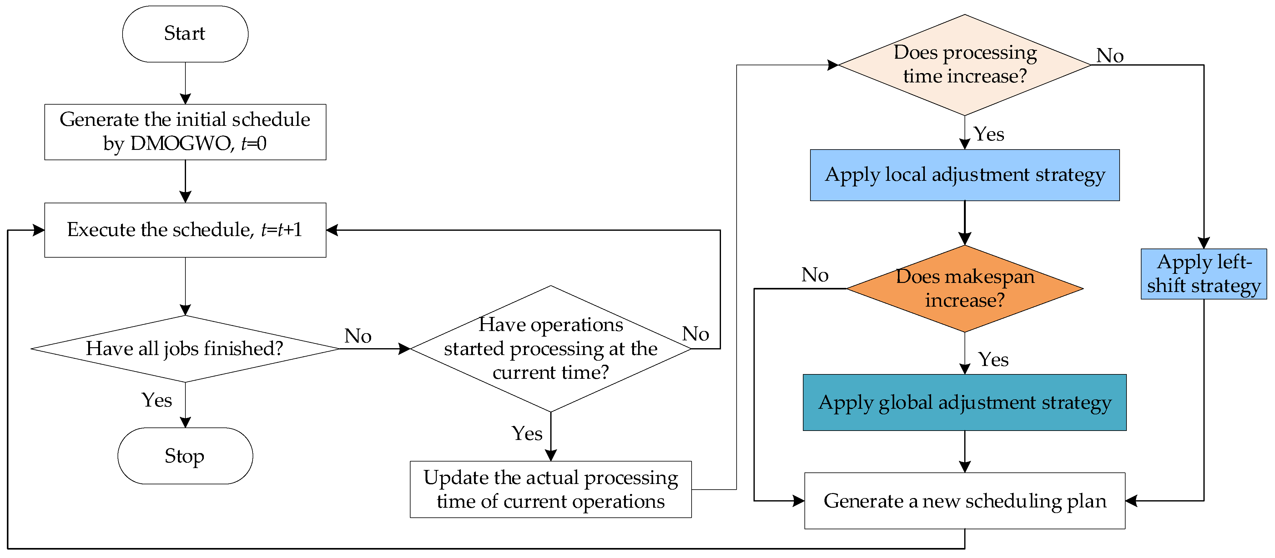
5.1. Framework of the Heuristic Scheduling Method

The flowchart of the heuristic scheduling method is summarized in Figure 1. Based on the predicted processing time outlined in Section 4, a robust initial scheduling plan is generated using DMOGWO considering three optimization objectives. Then, during the implementation of the schedule, the actual processing time of each operation is only determined when the operation is about to begin, bringing about a deviation in the estimated processing time. Consequently, a scheduling decision should be made at that time to make adjustments as the reaction to the change in processing time. In this study, a hybrid heuristic scheduling method that combines three adjustment strategies is proposed according to different scenarios with the aim of ensuring both the scheduling efficiency and robustness in uncertain production environments. The relevant description is as follows:

Strategy 1: If the processing time of the current operation is reduced or remains unchanged, no rescheduling is triggered. Instead, a left-shift adjustment is applied within the current factory to locally optimize the schedule.

Strategy 2: If the processing time of the current operation increases, the first, the binary tree [32] for the subsequent operations corresponding to the current operation is constructed. In this binary tree, the left node stores the subsequent processes belonging to the same workpiece, while the right node stores the subsequent processes allocated in the same machine. A local adjustment strategy based on insertion is applied to all operations in the tree. The new makespan in this factory is then calculated. The critical factory with the maximum makespan in the current schedule plays a decisive role in improving the overall scheduling efficiency. If the new makespan is smaller than that of the critical factory, no rescheduling is required.

Strategy 3: If the new makespan exceeds that of the critical factory, a DMOGWO-based global rescheduling method is triggered to schedule a new DFJSP. At each rescheduling point, the operations that are completed and being processed on the machine in the original schedule remain unchanged, while the remaining unprocessed operations are reassigned to new machines for sequencing to achieve global optimization.

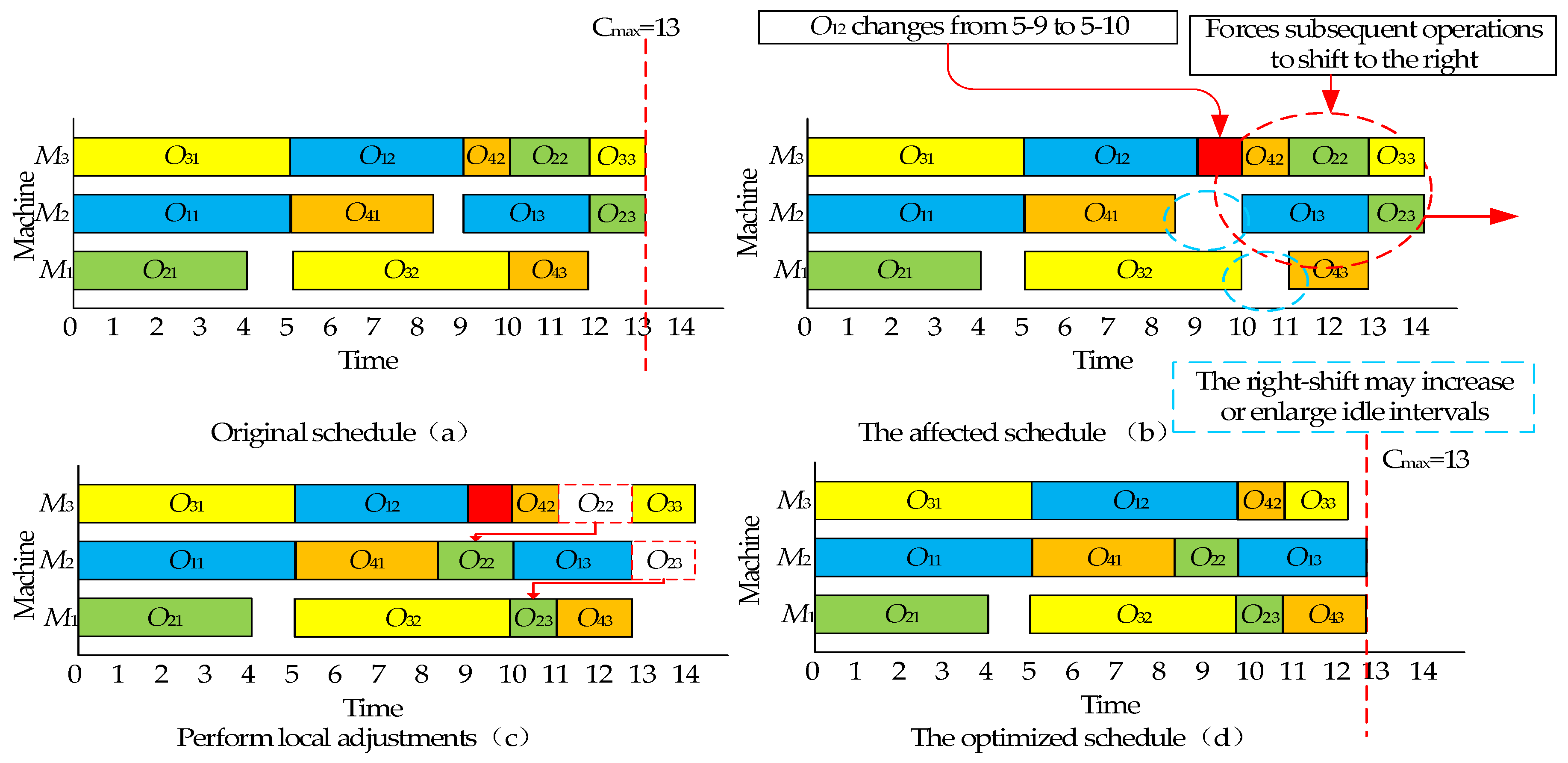
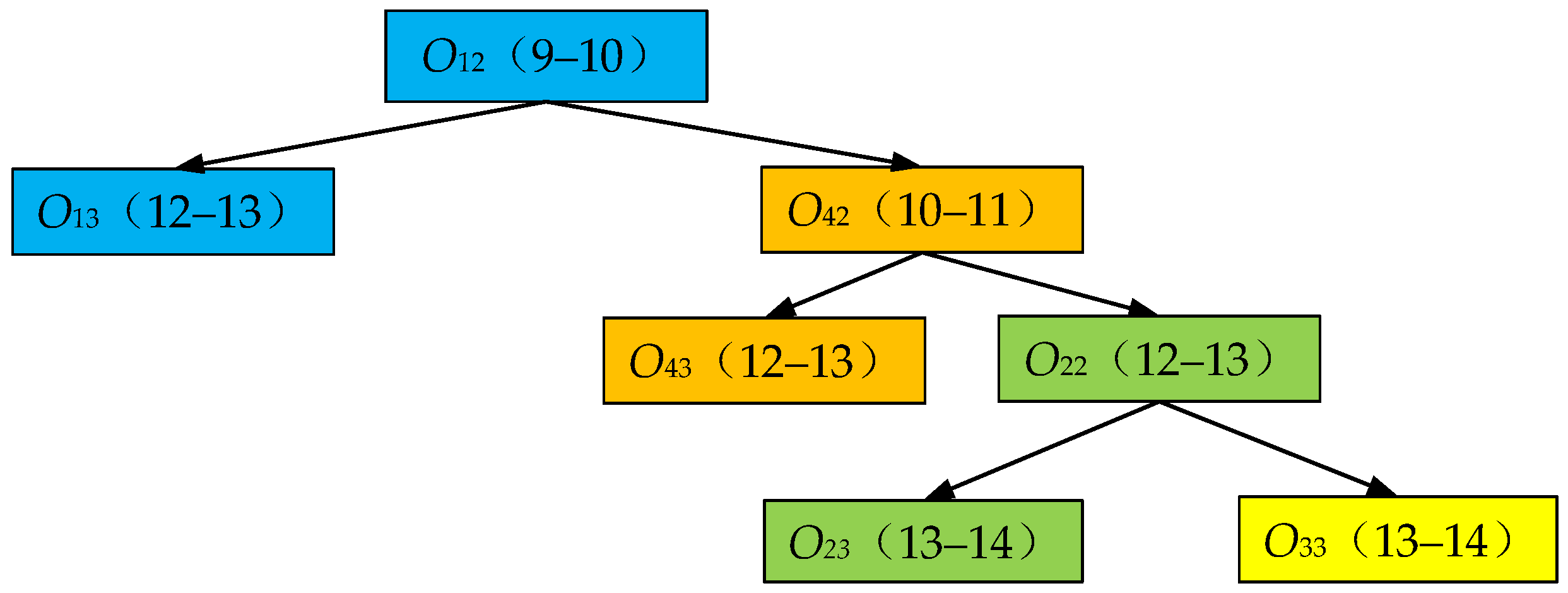
5.2. Insertion-Based Local Adjustment Strategy

To explain this strategy, an example as shown in Figure 2 is provided. With regard to the original scheduling in Figure 2a, when the processing time of an operation increases, it may delay the start time of its subsequent operations within the same job or those that are processed on the same machine, resulting in the right-shift phenomenon as shown in Figure 2b. This can lead to two issues: (1) the emergence of idle intervals in areas where none existed in the original schedule, and (2) the expansion of existing idle intervals. To address these issues, an insertion-based local adjustment strategy is proposed, and the specific steps are described as follows:

Step 1: Construct the binary tree for the operation with an increased processing time as shown in Figure 3. Each node represents an operation.

Step 2: Calculate the completion time after the right-shift for each node in the binary tree. As to the tree shown in Figure 3, the two values in the brackets which are labeled on each node represent the completion time of the corresponding operation before and after the right-shift, respectively.

Step 3: Traverse the binary tree layer by layer to handle each operation. Let $I^{lk}=[I_s^{lk},I_e^{lk}]$ be the valid idle interval on machine k in factory l beginning from $I_s^{lk}$ and ending at $I_e^{lk}$. For the current operation $O_{ij}$, evaluate all available idle intervals on its candidate machines. Let $S_{ij}^{*}$ be the start time of the operation following $O_{ij}$ within the same job and $C_{ij}^{*}$ be the completion time of the operation that precedes $O_{ij}$ within the same job. If an idle interval satisfies Equation (22), the operation is inserted into the corresponding machine; otherwise, no adjustment is made.

$$\max (C_{ij}^{*},I_s^{lk},t_l)+p_{ij}^{lk}\le \min (S_{ij}^{*},I_e^{lk}).$$

(22)

To demonstrate the effectiveness of the insertion-based local adjustment strategy, Figure 2 provides an example in which the processing time of operation $O_{12}$ increases from 4 to 5, causing its completion time to be delayed from 9 to 10. A binary tree for the subsequent operations of $O_{12}$ is then constructed, as illustrated in Figure 3. Figure 2b shows that all operations in the binary tree are affected, not only increasing the completion time but also potentially creating or enlarging idle intervals. To address this challenge, the operations in the binary tree are locally adjusted by attempting to insert them into available idle intervals on other machines, as shown in Figure 2c. The newly obtained schedule in Figure 2d shows that the overall makespan remains unchanged after the adjustment, which effectively demonstrates that a reasonable local adjustment strategy can respond to variable processing times and maintain product planning to some extent.

5.3. DMOGWO-Based Global Adjustment Strategy

It is notable that the original GWO is designed for continuous optimization problems, while the DDFJSP-VPT is a multi-objective combinational optimization problem. Thus, we modify the GWO to develop DMOGWO according to the features of the DDFJSP-VPT and multi-objective optimization by designing the encoding and decoding schemes, as well as the searching operators. Its framework is illustrated in Algorithm 1. The algorithm begins by initializing the population and performing non-dominated sorting [33] to identify the leader wolf packs. Then, steps 4 to 18 are iterated until the termination criterion is satisfied. In each generation t, each wolf in the population independently selects a leader from the leading wolves to follow. The wolf pack is updated through discretized crossover and mutation operations to generate new individuals. Finally, the parent and offspring populations are merged, and the next generation of wolves, along with new leader wolf packs, are selected.

Algorithm 1: Framework of the DMOGWO algorithm

1: Initialize a wolf group P0

2: Determine leader wolf packs according to non-dominated sorting

3: t = 0

4: while (stop criterion is not satisfied) do

5:    Pnew = Ø

6:    for each wolf St ∈ Pt do

7:     determine Sα, Sβ, Sδ as Sleader from leader wolf packs

8:     off ← Crossover (St, Sleader)

9:     if rand < Pm then

10:        off ← Mutation (off)

11:    end if

12:     Pnew ← Pnew ∪ off

13:    end for

14:    {F1, F2, …, Flast} ← Non-dominated sorting and crowding distance(Pt ∪ Pnew)

15:    Pt+1 ← Environmental Selection (F1,F2,…,Flast)

16:    Determine leader wolf packs according to different ranks

17:    t = t + 1

18: end while

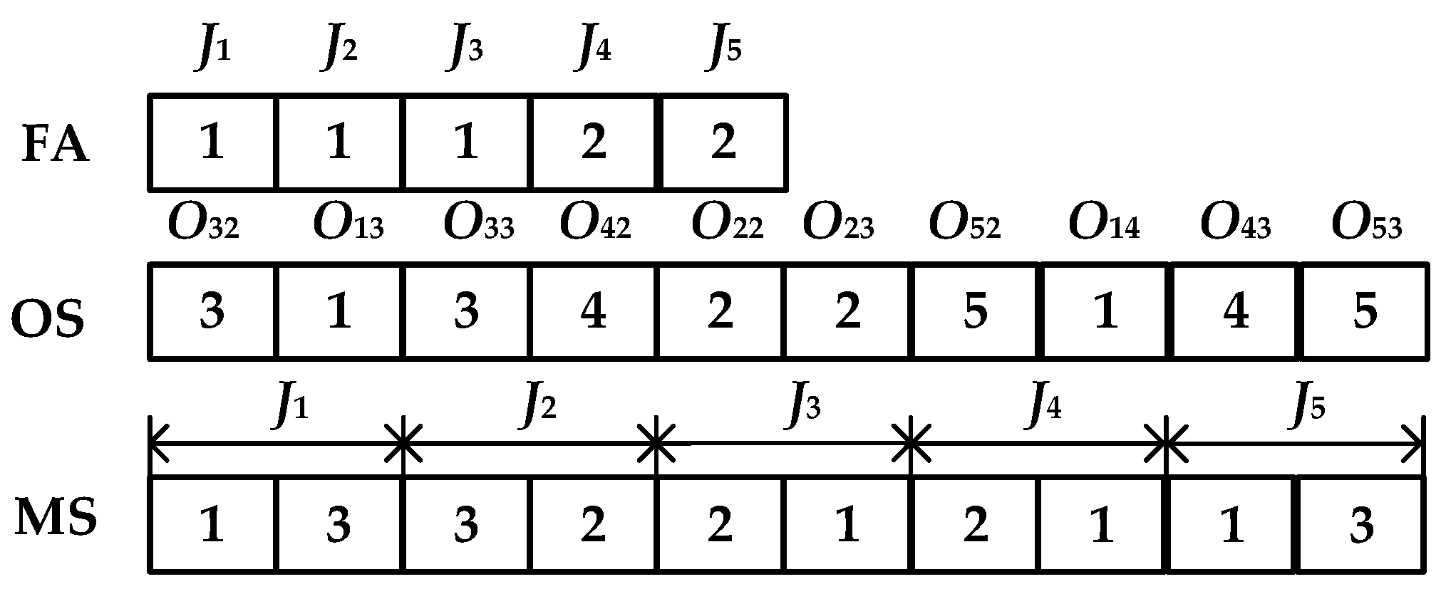
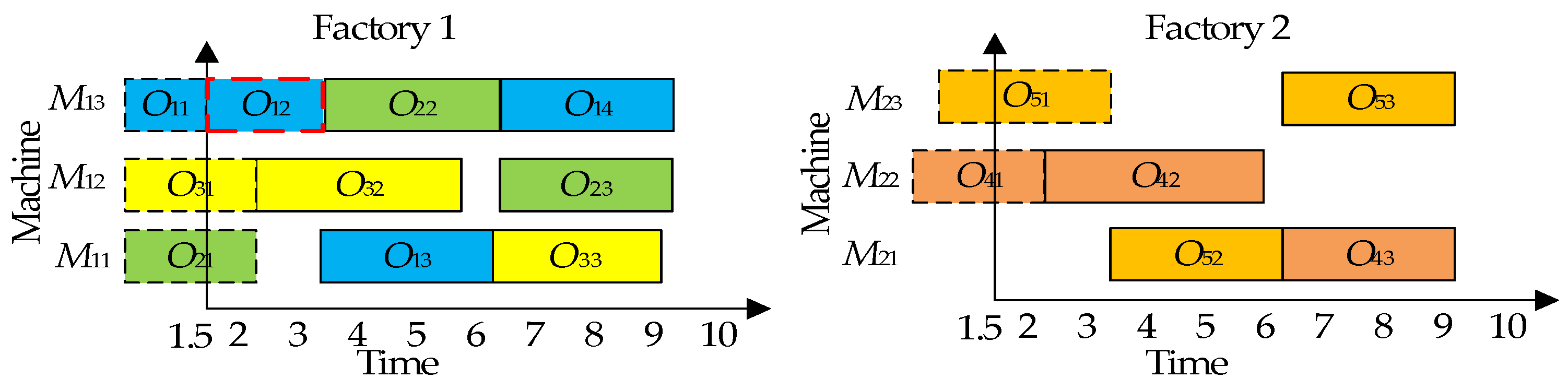
5.3.1. Chromosome Encoding

In the context of scheduling problems, an encoding method is used as an effective means of transforming the scheduling problem into a representation within the search space. A well-designed encoding scheme ensures the adequacy of the search space and enhances the efficiency of the problem-solving process. Given the characteristics of the DDFJSP-VPT, a three-layer encoding scheme including factory assignment (FA), operation sequence (OS), and machine selection (MS) is adopted in the proposed DMOGWO, representing each individual as S = [FA,MS,OS]. It must be noted that the length of the chromosome is variable rather than fixed, because the number of scheduled operations is constantly changing throughout the whole manufacturing process. The details are as follows:

Factory Assignment (FA): FA represents the assignment of each job to a specific factory for processing. As illustrated in Figure 4, five jobs must be assigned to two factories. The first number, “1”, in the FA indicates that job $J_1$ is assigned to factory $U_1$. The length of the FA corresponds to the total number of jobs, ensuring that each job is allocated to a specific factory. It should be noted that the factory assignment remains fixed for jobs that have already started processing.

Operation Sequence (OS): OS determines the processing sequence of operations for each job. It assumes that, at a specific rescheduling point, O₁₂ is the operation whose processing time is currently changing and will not be rescheduled. The operations O₁₃, O₁₄, O₂₂, O₂₃, O₃₂, O₃₃, O₄₂, O₄₃, O₅₂, O₅₃ are left unprocessed from the previous schedule. Therefore, the OS contains the job numbers 1, 2, 3, 4, and 5, and the sequence in which an integer appears indicates the operation sequence of a job. Thus, the operation sequence vector can be interpreted as O₃₂ → O₁₃ → O₃₃ → O₄₂ → O₂₂ → O₂₃ → O₅₂ → O₁₄ → O₄₃ → O₅₃.

Machine Selection (MS): MS represents the assignment of operations to specific machines for processing. The numbers in the MS indicate the machine selected for each operation within the assigned factory. The length of the MS matches the total number of operations, following the order of jobs and their respective operations. For instance, the first number “1” in the MS indicates that operation $O_{13}$ is assigned to machine $M_{11}$ in factory $U_1$ for processing.

5.3.2. Chromosome Decoding

In the decoding process, the FA is first used to determine the sequence of operations assigned to each factory. Then, for each factory, the sequence of operations and their corresponding machine assignments are treated as an FJSP. The insertion method proposed by Gao et al. [34] is used to decode the sequence and generate an active schedule, ensuring that operations are processed as early as possible without increasing the machine load. The decoding steps for each factory are as follows:

Step 1: Traverse the OS within the current factory to identify the factory $U_l$ and machine $M_{lk}$ corresponding to each operation $O_{ij}$ and then calculate the theoretical processing time $p_{ij}^{lk}$.

Step 2: Check the available time slots $I^{lk}=[I_s^{lk},I_e^{lk}]$ for machine $M_{lk}$ from the earliest to the latest. If a time slot satisfies Equation (22), insert the operation into the corresponding machine’s position. If no available time slots can accommodate the operation, place it at the end of the machine’s position.

Step 3: Once all operations within the current factory have been processed, update the OS based on their start times. If not all operations have been processed, go to Step 1 until all operations are processed on their corresponding machine.

Figure 5 gives a corresponding decoding diagram of the chromosome represented in Figure 4.

5.3.3. Population Initialization

To generate a high-quality initial population and ensure a solid foundation for the subsequent optimization process, we propose a hybrid initialization strategy that combines multiple heuristic rules. During the initialization process, FA is generated first, followed by OS, and finally MS. The detailed procedure is as follows:

For FA: The initialization strategy for FA incorporates two approaches. The first approach prioritizes factories with fewer assigned operations. The second approach selects a factory randomly. We use two strategies with equal proportions to ensure load balancing and diversity in the factory allocations.

For OS: The operation sequence is generated randomly to promote the exploration of the search space, providing a broad set of initial solutions for further optimization.

For MS: The initialization of machine assignments is performed using the following four strategies: (1) machines are arranged in ascending order based on the number of available processing machines for each operation, and the machine with the smallest workload in the current factory is prioritized. (2) The assigned operations in a factory are decoded into an active schedule according to the partial OS and MS code. Then, the insertion is attempted for the current operation to find the machine from the candidate machine set that achieves the shortest completion time. Once the insertion fails, the machine with the earliest completion time at present is chosen. (3) The machine with the shortest processing time for the operation is selected. (4) Machines are selected randomly. The probability of these strategies being selected is equal.

5.3.4. Social Structure of the Wolf Pack

Considering that this study focuses on a multi-objective optimization problem, the fixed population structure used in the traditional GWO algorithm can easily lead to premature convergence. To address this issue, the method proposed in [35] is adopted to select the leader wolves. The detailed approach is as follows:

• If the population consists of a single non-dominated rank, the leader wolves $S_{\alpha }$, $S_{\beta }$, and $S_{\delta }$ are randomly selected from this rank.
• If the population has two non-dominated ranks, $S_{\alpha }$ is randomly selected from the first rank, while $S_{\beta }$ and $S_{\delta }$ are chosen randomly from the second rank.
• If the population contains more than two non-dominated ranks, $S_{\alpha }$, $S_{\beta }$, and $S_{\delta }$ are randomly selected from the first, second, and third ranks, respectively.

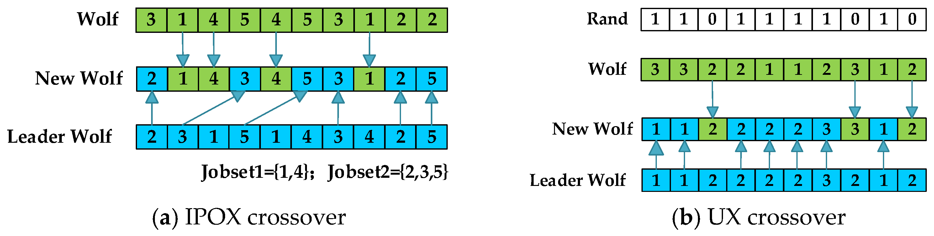
5.3.5. Wolf Pack Position Update Method

Since DMOGWO employs discrete encoding, the traditional position update method of the GWO algorithm is no longer suitable. Therefore, a crossover–mutation-based approach is introduced for updating the positions of the wolf pack. When using this method, each wolf reselects its leaders according to the procedure outlined in Section 5.3.4. The position update is then carried out using the crossover described as follows:

$$off=\left\{\begin{array}{ll}\mathrm{Crossover}(S_{\alpha },S),& if rand < 1/3\\ \mathrm{Crossover}(S_{\beta },S),& if 1/3 \le rand < 2/3\\ \mathrm{Crossover}(S_{\delta },S),& \mathrm{otherwise}\end{array}\right..$$

(23)

Considering the adaptation to the coding scheme, three different crossover operators are proposed for FA, OS, and MS. A single-point crossover is employed for FA. A random number n* is generated between 0 and n. The first n* jobs of the FA encoding are inherited from the leader wolf, while the remaining jobs are inherited from a regular wolf. The IPOX [36] and UX [37] operators are applied to the OS and MS, respectively, as illustrated in Figure 6.

For the mutation, a single-point mutation is applied to FA, where one job is randomly selected, and its associated factory is changed. As for OS, it is achieved by swapping the positions corresponding to two randomly selected operations. With regard to the MS, a two-point mutation is adopted, in which two operations are randomly selected, and their associated machines are altered. In Figure 7, the above two-point and swap mutations are illustrated. Additionally, the mutation probability Pm is set to 0.15 in this study.

6. Experiments and Results

The proposed method is implemented in MATLAB 2016b and runs on an Intel Core i7 @ 2.90 GHz computer with 16 GB RAM (Intel, Santa Clara, CA, USA). These experiments aim to evaluate the efficiency and robustness of our proposed method in addressing the DDFJSP-VPT.

6.1. Experimental Instances and Processing Time Variability

To validate the effectiveness of the proposed method, the classic benchmark instances MK01–10 [38] are extended to a two-factory environment. The scale of MK01–10 is shown in

Table 2. Problem instances.

Instance	Number of Jobs	Number of Machines	Operations Range per job	Machines Range per Operation	Time Range per Operation
MK01	10	6	5–7	3	1–7
MK02	10	6	5–7	6	1–7
MK03	15	8	10–10	5	1–20
MK04	15	8	3–10	3	1–10
MK05	15	4	5–10	2	5–10
MK06	15	15	15–15	5	1–10
MK07	20	5	5–5	5	1–20
MK08	20	10	10–5	2	5–20
MK09	20	10	10–15	5	5–20
MK10	20	15	10–15	5	5–20

. In this study, processing times are assumed to follow a normal distribution, where the theoretical processing time $p_{ij}^{lk}$ provided in the benchmark instance is treated as the mean processing time ${\mu }_{ij}^{lk}$ for each operation, and the variance is defined as a fraction $\kappa$ of the mean. Different variances will lead to fluctuations of varying degrees. To maintain a manageable level of problem complexity while reflecting real-world characteristics, the $\kappa$-value corresponding to “low variability” defined in [21] is selected—specifically $\kappa$ = 0.1.

Although the variability of processing times remains consistent across all instances, the theoretical processing times differ between instances. Different theoretical processing times lead to varying fluctuation amplitudes because the variance is calculated as a proportion of the theoretical time. As a result, the actual fluctuation amplitude of processing times differs across instances, which directly affects the choice of scheduling strategy. For example, operations with larger fluctuations in processing times require more flexible scheduling strategies to accommodate the larger impact, while operations with smaller fluctuations can be handled with simpler scheduling approaches. The relevant scheduling strategies and details are discussed in Section 5.1 of the paper.

Furthermore, to ensure fair comparisons among all algorithms, a unified termination criterion is adopted by setting the maximum number of function evaluations as $600\times {\displaystyle \sum _{i=1}^n{n}_i}$. The code and the data can be downloaded from: https://github.com/Gaiboom/code-and-data-for-DDFJSP-VPT (accessed on 3 February 2025).

6.2. Experimental Metrics

To comprehensively evaluate the performance of the algorithms, the HV [39], IGD [40], and C [41] metrics are used as indicators in our experiments.

(1) The inverted generational distance (IGD) evaluates both the convergence and diversity of the obtained solutions. It is defined as the average Euclidean distance from each point in the true Pareto front $P{F}^{True}$ to its nearest solution in the Pareto front $P{F}^A$ obtained by algorithm A. The IGD is computed as:

$$IGD(A)={\displaystyle \frac{{\displaystyle {\sum }_{i=1}^{\left|P{F}^{True}\right|}\left|d_i^{*}\right|}}{\left|P{F}^{True}\right|}},$$

(24)

where $\left|P{F}^{True}\right|$ is the numbers of points in $P{F}^{True}$, $d_i^{*}$ is the Euclidean distance from the ith point of the $P{F}^{True}$ to the nearest point of the $P{F}^A$.

(2) The C metric is used to compare the dominance relationship between the non-dominated solution sets of two algorithms. Its calculation method is given in Equation (25).

$$C(A,B)={\displaystyle \frac{\left|\right\{b\in B:\exists a\in A,a\succ b\left\}\right|}{\left|B\right|}},$$

(25)

where $C(A,B)$ measures the proportion of solutions in B dominated by those in A, with $\left|B\right|$ representing the total number of solutions in B.

(3) The hypervolume (HV) metric is used to measure both the convergence and diversity of the obtained Pareto front by computing the volume in the objective space that is dominated by the solution set and bounded by a reference point. The HV is computed as:

$$HV(A,z)=vol\left(\cup \left[f_1,z_1\right]\times \dots \left[f_n,z_n\right]\right),$$

(26)

where z is the reference point. The hypervolume $HV(A,z)$ quantifies the volume of the objective space dominated by the solution set.

Specifically, the smaller the IGD value, the better the algorithm’s performance. In contrast, the greater the HV and C values, the better the performance of the algorithm. Note that HV and IGD can reflect the comprehensive performance, while C can only measure the convergence of algorithms to some extent. The reference set used for IGD is obtained by merging the non-dominated solutions from all algorithms and extracting the non-dominated solutions from this merged set. The objective values of the non-dominated solutions from all algorithms are normalized using Equation (24):

$${\tilde{f}}_i(x)={\displaystyle \frac{\left(f_i(x)-f_i^{\min }\right)}{\left(f_i^{\max }-f_i^{\min }\right)}}, i=1,2,3,$$

(27)

where $f_i^{\min }$ and $f_i^{\max }$ represent the minimum and maximum values among all solution sets, respectively. Thus, the reference point for calculating HV is set to (1.1,1.1,1.1) ^T.

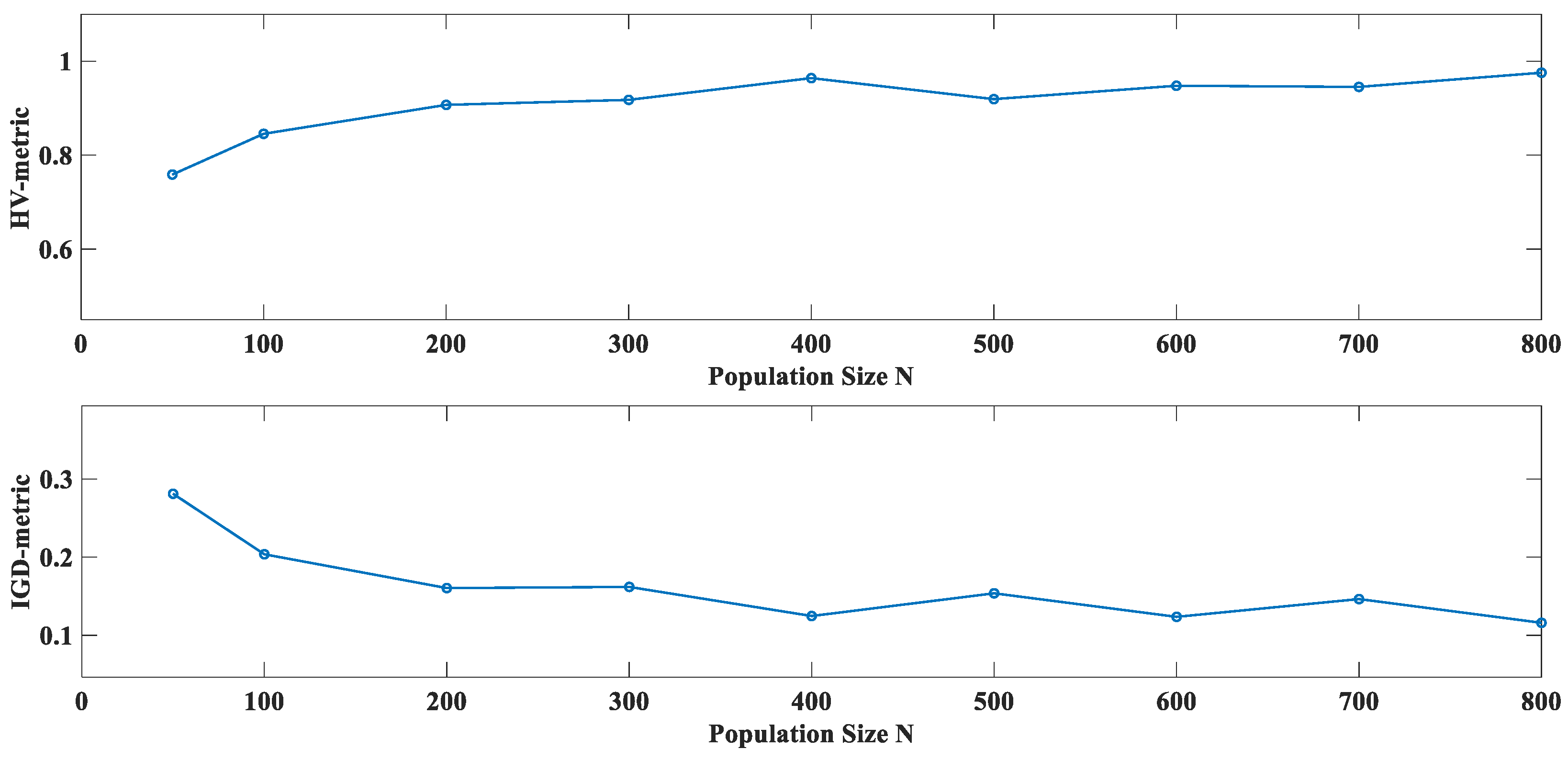
6.3. Sensitivity Analysis of Population Size

Our DMOGWO algorithm has one key parameter, namely the population size N. To investigate the impact of different N values on the algorithm’s performance, nine levels of N are selected from the range [50,800], and the MK08 instance is tested. Each level independently runs 10 times, and the average HV and IGD values are computed. The influence of the key parameter N on the algorithm’s performance is illustrated in Figure 8. It can be observed that DMOGWO is not very sensitive to the setting of N under the ranges considered, which effectively shows the algorithm’s stability and robustness. Considering the balance between the number of evenly distributed solutions and the computational cost, the population size N is ultimately set to 200 in this study.

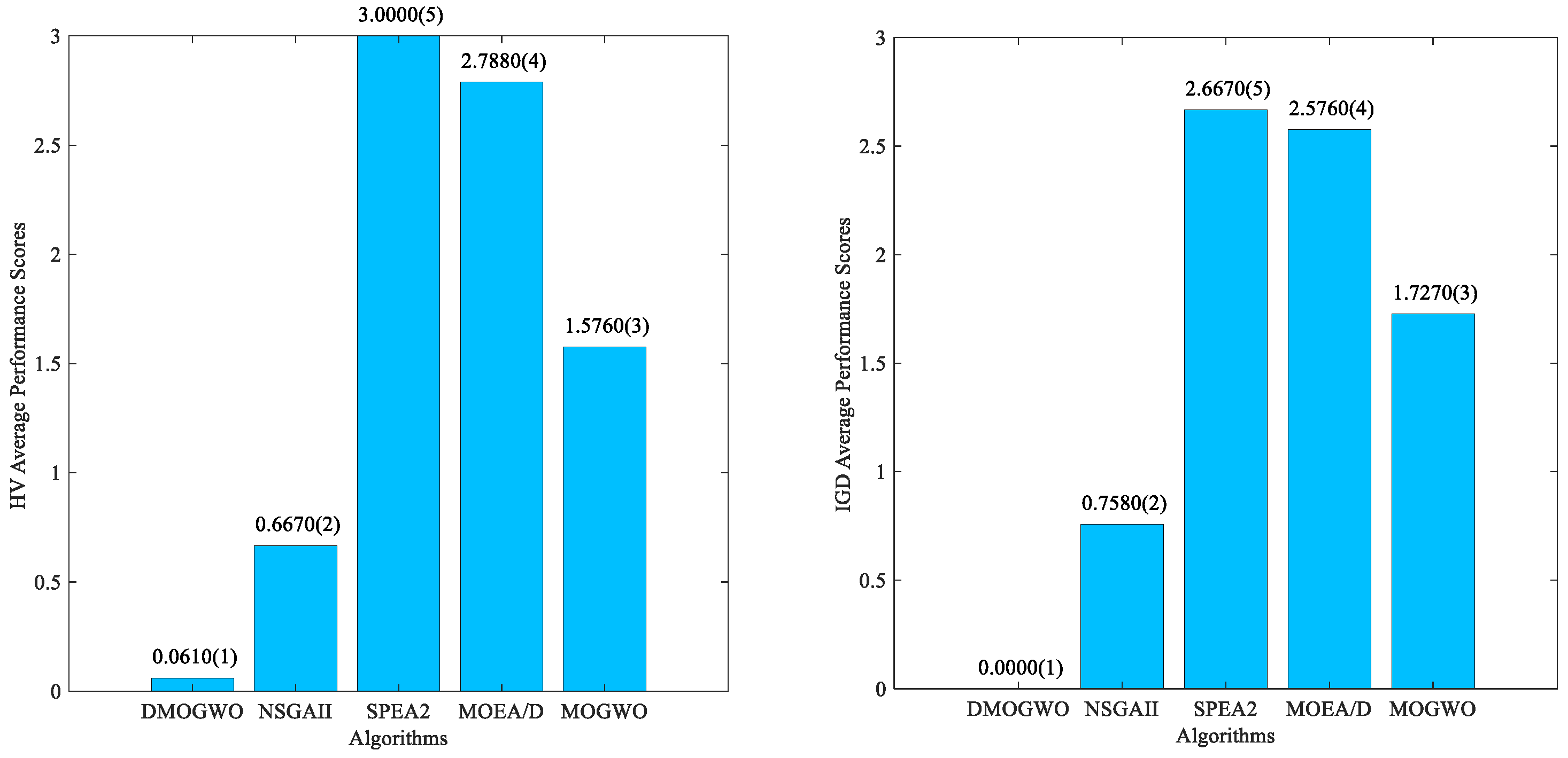
6.4. Performance Evaluation of the DMOGWO Algorithm

The proposed DMOGWO-based rescheduling algorithm is compared with four other algorithms, namely, NSGA-II [33], MOEA/D [42], SPEA2 [43], and MOGWO [8], with respect to the static and dynamic aspects of the problem, in order to evaluate their overall performance. The reasons for selecting these compared algorithms are as follows: (1) NSGA-II, SPEA2, and MOGWO share a similar structure with the proposed DMOGWO, as they are all non-dominated sorting-based multi-objective optimization algorithms, whereas MOEA/D adopts a decomposition strategy for optimization, providing a different optimization paradigm for comparison. (2) NSGA-II, SPEA2, and MOEA/D have been widely used in the field of production scheduling, and their effectiveness in multi-objective scheduling optimization has been well-validated, making them reliable benchmark algorithms. (3) MOGWO, designed for multi-objective flexible scheduling, is based on GWO, making it closely related to our DMOGWO. As a more recent algorithm, MOGWO allows comparison with both classical and modern swarm intelligence techniques, ensuring a comprehensive performance evaluation.

To ensure fairness, the traditional multi-objective evolutionary algorithms NSGA-II, MOEA/D, and SPEA2 are configured with the same population size and mutation probability as DMOGWO. For MOGWO, which has been successfully applied to the FJSP, the parameter settings are adopted as described in the original paper. All comparative algorithms utilized the same initialization strategy.

6.4.1. Performance Comparisons in the Initial Static Problem

This section focuses on the static DFJSP without variable processing times to comprehensively evaluate the performance of the proposed algorithm. All comparative algorithms are independently run 20 times on each benchmark instance, and the average HV, IGD, and C values are computed. A Wilcoxon signed-rank test [44] with a significance level of 0.05 is carried out to assess the significant differences in the results. The Wilcoxon test is a non-parametric statistical method that does not rely on distributional assumptions and is effective in assessing significant differences between algorithms. In

Table 3. Comparison between DMOGWO and other algorithms using HV and IGD values.

Instance	HV					IGD
	DMOGWO	NSGA-II	SPEA2	MOEA/D	MOGWO	DMOGWO	NSGA-II	SPEA2	MOEA/D	MOGWO
MK01	1.1540	1.1710 (=)	1.1023 (=)	0.9855 (+)	1.1375 (=)	0.0961	0.1153 (=)	0.1356 (=)	0.2074 (+)	0.1110 (=)
MK02	1.1931	1.2018 (=)	1.1931 (=)	1.0917 (+)	1.1828 (=)	0.0606	0.0691 (=)	0.0717 (=)	0.1428 (+)	0.0660 (=)
MK03	1.1957	1.1864 (=)	0.8034 (+)	1.0246 (+)	1.1695 (+)	0.0054	0.0106 (+)	0.1285 (+)	0.0713 (+)	0.0173 (+)
MK04	1.2296	1.2200 (=)	0.8787 (+)	1.0839 (+)	1.1936 (+)	0.0269	0.0284 (=)	0.1871 (+)	0.1038 (+)	0.0410 (+)
MK05	1.2017	1.1597 (+)	0.9441 (+)	0.8984 (+)	1.0950 (+)	0.0798	0.0870 (=)	0.1849 (+)	0.2087 (+)	0.1181 (+)
MK06	0.9401	0.9308 (=)	0.6488 (+)	0.6670 (+)	0.8155 (+)	0.1009	0.1244 (=)	0.2416 (+)	0.4040 (+)	0.2064 (+)
MK07	1.1766	1.1614 (=)	0.9137 (+)	0.9957 (+)	1.0828 (+)	0.0581	0.0603 (=)	0.1621 (+)	0.1264 (+)	0.1023 (+)
MK08	1.0795	1.0231 (+)	0.6900 (+)	0.7983 (+)	0.8964 (+)	0.1546	0.1864 (+)	0.3765 (+)	0.2664 (+)	0.2419 (+)
MK09	1.1729	1.1435 (+)	0.8046 (+)	0.9028 (+)	1.0436 (+)	0.0470	0.0657 (+)	0.2167 (+)	0.1705 (+)	0.1215 (+)
MK10	1.2095	1.1896 (+)	0.9888 (+)	1.0388 (+)	1.1530 (+)	0.0292	0.0448 (+)	0.1447 (+)	0.1421 (+)	0.0805 (+)

,

Table 4. Comparison between DMOGWO and other algorithms using C values.

Instance	DMOGWO(A) vs. NSGA-II(B)		DMOGWO(A) vs. SPEA2(C)		DMOGWO(A) vs. MOEA/D(D)		DMOGWO(A) vs. MOGWO(E)
	C(A,B)	C(B,A)	C(A,C)	C(C,A)	C(A,D)	C(D,A)	C(A,E)	C(E,A)
MK01	0.3510	0.1023 (=)	0.4863	0.2005 (=)	0.8003	0.0500 (+)	0.4998	0.0508 (+)
MK02	0.3493	0.2493 (=)	0.2500	0.1993 (=)	0.8743	0.0000 (+)	0.1505	0.2490 (=)
MK03	0.5139	0.1800 (+)	0.7280	0.0020 (+)	0.9120	0.0000 (+)	0.9221	0.0153 (+)
MK04	0.3998	0.3409 (=)	0.5450	0.0139 (+)	0.9896	0.0013 (+)	0.8029	0.0482 (+)
MK05	0.4897	0.1953 (=)	0.8113	0.0540 (+)	1.0000	0.0000 (+)	0.8153	0.0043 (+)
MK06	0.6443	0.2040 (+)	0.7053	0.0533 (+)	0.9483	0.0015 (+)	0.8963	0.0520 (+)
MK07	0.4985	0.1663 (+)	0.8110	0.0000 (+)	0.9406	0.0000 (+)	0.9034	0.0088 (+)
MK08	0.5628	0.2493 (+)	0.7720	0.0008 (+)	0.9643	0.0040 (+)	0.9578	0.0013 (+)
MK09	0.4925	0.2305 (+)	0.8505	0.0010 (+)	0.9256	0.0003 (+)	0.9530	0.0098 (+)
MK10	0.5868	0.1933 (+)	0.7725	0.0492 (+)	0.9970	0.0000 (+)	0.9608	0.0033 (+)

, Table 5 and Table 6, the signs “+/−/=” indicate that DMOGWO performs significantly better than the compared algorithm, significantly worse than the compared algorithm, or shows no significant difference to the compared algorithm, respectively. The best values are highlighted in bold but it is important to note that bold values indicate only the best numerical performance, not necessarily statistical significance. The results are presented in Table 3 and Table 4.

Table 3 and Table 4 demonstrate that DMOGWO achieves optimal results for the HV, IGD, and C metrics in the majority of instances, as highlighted in bold. These results underline its superior performance in solving the static MODFJSP. Specifically, for the HV metric, while DMOGWO shows slightly lower values than NSGA-II on instances MK01 and MK02, the differences are not statistically significant, indicating comparable performances in these cases. Similarly, for the C metric, DMOGWO performs slightly worse than MOGWO on MK02, but the difference also fails to reach statistical significance. In comparison to MOGWO, DMOGWO has several advantages. First, DMOGWO employs a unique social hierarchy strategy where each wolf selects different leader wolves, whereas MOGWO uses a fixed leader wolf for all individuals, which can lead to local convergence. Second, DMOGWO adopts a discrete encoding and position update mechanism that better fits the static MODFJSP, while MOGWO combines continuous and discrete encoding, which may not fully capture the problem’s discrete characteristics.

Overall, despite its comparable or slightly inferior performance in certain instances, DMOGWO demonstrates a more balanced performance across the three key metrics, generating higher-quality Pareto solutions. These findings confirm the effectiveness of DMOGWO in addressing the static MODFJSP.

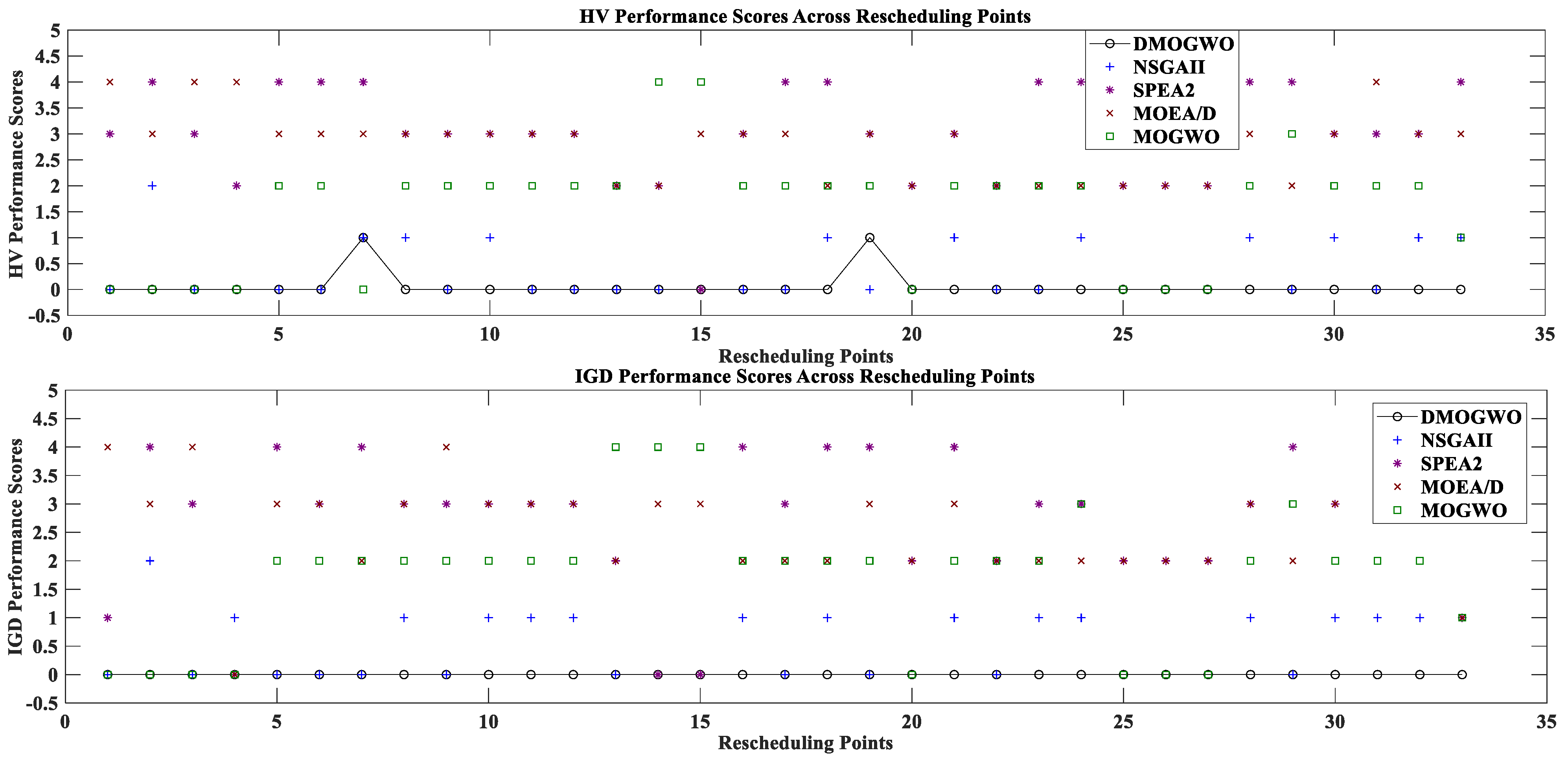
6.4.2. Performance Comparisons for the Dynamic Problem

This section presents a comparative analysis of the performance of different algorithms for the dynamic process of the DDFJSP-VPT for all instances. As each instance includes a varying number of rescheduling points, this study adopts the methodology outlined in [45]. For each rescheduling point, each algorithm is executed independently 20 times. The non-dominated solutions from these runs are combined, and the resulting non-dominated set is used as the reference Pareto front to calculate the performance metrics of each algorithm at each rescheduling point. The performance metrics across all rescheduling points in each run are then aggregated and averaged, yielding 20 average results that represent the algorithm’s performance over the entire dynamic process of the instance. Finally, these 20 averages are further averaged to compute the overall performance values for each algorithm in the corresponding instance. The results are presented in Table 5 and Table 6.

The experimental results demonstrate that DMOGWO exhibits excellent optimization performance in addressing the DDFJSP-VPT. As shown in Table 5, DMOGWO achieves the highest HV values in 6 out of 10 instances and the lowest IGD values in 8 out of 10 instances, significantly outperforming other algorithms in most cases, with no instances of values that are significantly inferior to others. Furthermore, in terms of the C metric, DMOGWO consistently surpasses SPEA2, MOEA/D, and MOGWO across the majority of instances. Additionally, when compared with MOEA/D and MOGWO, the C values approximate 1 in some instances, indicating that its solution set almost completely dominates these two algorithms. These findings validate DMOGWO’s ability to generate Pareto fronts with better convergence and distribution in dynamic scheduling problems.

Table 5. Comparison between DMOGWO and other algorithms using HV and IGD values.

Instance	HV					IGD
	DMOGWO	NSGA-II	SPEA2	MOEA/D	MOGWO	DMOGWO	NSGA-II	SPEA2	MOEA/D	MOGWO
MK01	0.7738	0.7603 (=)	0.7069 (+)	0.6521 (+)	0.7827 (=)	0.0199	0.0281 (=)	0.0810 (+)	0.1016 (+)	0.0294 (=)
MK02	0.7362	0.6903 (+)	0.6421 (+)	0.5926 (+)	0.7433 (=)	0.0536	0.0699 (=)	0.0767 (+)	0.1154 (+)	0.0502 (=)
MK03	1.2031	1.2032 (=)	0.8313 (+)	1.0458 (+)	1.1829 (+)	0.0114	0.0138 (=)	0.1450 (+)	0.0713 (+)	0.0254 (+)
MK04	0.7616	0.7588 (=)	0.5943 (+)	0.6655 (+)	0.7495 (+)	0.0141	0.0153 (=)	0.0848 (+)	0.0661 (+)	0.0310 (+)
MK05	1.2028	1.1762 (+)	0.9385 (+)	0.9083 (+)	1.0734 (+)	0.0487	0.0622 (+)	0.1579 (+)	0.1776 (+)	0.1188 (+)
MK06	0.8062	0.8098 (=)	0.7011 (+)	0.6305 (+)	0.6290 (+)	0.0449	0.0402 (=)	0.1082 (+)	0.2068 (+)	0.2008 (+)
MK07	1.0272	0.9310 (+)	0.6847 (+)	0.7477 (+)	0.9003 (+)	0.0282	0.0399 (+)	0.1691 (+)	0.1240 (+)	0.1036 (+)
MK08	0.7434	0.6699 (+)	0.5093 (+)	0.5493 (+)	0.6314 (+)	0.0391	0.0523 (+)	0.1373 (+)	0.1116 (+)	0.1193 (+)
MK09	1.1828	1.1618 (+)	0.8553 (+)	1.0261 (+)	1.0592 (+)	0.0249	0.0362 (+)	0.2166 (+)	0.1188 (+)	0.1233 (+)
MK10	0.9470	0.9171 (+)	0.7176 (+)	0.7122 (+)	0.8573 (+)	0.0966	0.1132 (+)	0.1949 (+)	0.2087 (+)	0.1508 (+)

Table 5. Comparison between DMOGWO and other algorithms using HV and IGD values.

Instance	HV					IGD
	DMOGWO	NSGA-II	SPEA2	MOEA/D	MOGWO	DMOGWO	NSGA-II	SPEA2	MOEA/D	MOGWO
MK01	0.7738	0.7603 (=)	0.7069 (+)	0.6521 (+)	0.7827 (=)	0.0199	0.0281 (=)	0.0810 (+)	0.1016 (+)	0.0294 (=)
MK02	0.7362	0.6903 (+)	0.6421 (+)	0.5926 (+)	0.7433 (=)	0.0536	0.0699 (=)	0.0767 (+)	0.1154 (+)	0.0502 (=)
MK03	1.2031	1.2032 (=)	0.8313 (+)	1.0458 (+)	1.1829 (+)	0.0114	0.0138 (=)	0.1450 (+)	0.0713 (+)	0.0254 (+)
MK04	0.7616	0.7588 (=)	0.5943 (+)	0.6655 (+)	0.7495 (+)	0.0141	0.0153 (=)	0.0848 (+)	0.0661 (+)	0.0310 (+)
MK05	1.2028	1.1762 (+)	0.9385 (+)	0.9083 (+)	1.0734 (+)	0.0487	0.0622 (+)	0.1579 (+)	0.1776 (+)	0.1188 (+)
MK06	0.8062	0.8098 (=)	0.7011 (+)	0.6305 (+)	0.6290 (+)	0.0449	0.0402 (=)	0.1082 (+)	0.2068 (+)	0.2008 (+)
MK07	1.0272	0.9310 (+)	0.6847 (+)	0.7477 (+)	0.9003 (+)	0.0282	0.0399 (+)	0.1691 (+)	0.1240 (+)	0.1036 (+)
MK08	0.7434	0.6699 (+)	0.5093 (+)	0.5493 (+)	0.6314 (+)	0.0391	0.0523 (+)	0.1373 (+)	0.1116 (+)	0.1193 (+)
MK09	1.1828	1.1618 (+)	0.8553 (+)	1.0261 (+)	1.0592 (+)	0.0249	0.0362 (+)	0.2166 (+)	0.1188 (+)	0.1233 (+)
MK10	0.9470	0.9171 (+)	0.7176 (+)	0.7122 (+)	0.8573 (+)	0.0966	0.1132 (+)	0.1949 (+)	0.2087 (+)	0.1508 (+)

Table 6. Comparison between DMOGWO and other algorithms using C metric values.

Instance	DMOGWO(A) vs. NSGA-II(B)		DMOGWO(A) vs. SPEA2(C)		DMOGWO(A) vs. MOEA/D(D)		DMOGWO(A) vs. MOGWO(E)
	C(A,B)	C(B,A)	C(A,C)	C(C,A)	C(A,D)	C(D,A)	C(A,E)	C(E,A)
MK01	0.5935	0.1726 (+)	0.5529	0.1225 (+)	0.8733	0.0013 (+)	0.5433	0.2716 (=)
MK02	0.3980	0.1988 (=)	0.3878	0.1490 (+)	0.7365	0.0741 (+)	0.2245	0.2506 (=)
MK03	0.3518	0.2705 (=)	0.7693	0.0053 (+)	0.9975	0.0000 (+)	0.8019	0.0615 (+)
MK04	0.2371	0.1816 (=)	0.3468	0.0085 (+)	0.7244	0.0020 (+)	0.8439	0.0273 (+)
MK05	0.5026	0.2026 (+)	0.6285	0.0110 (+)	0.9455	0.0000 (+)	0.9486	0.0016 (+)
MK06	0.4142	0.4544 (=)	0.5509	0.2141 (+)	0.9366	0.0132 (+)	0.9973	0.0008 (+)
MK07	0.3051	0.1891 (=)	0.6516	0.0036 (+)	0.8308	0.0031 (+)	0.7515	0.0037 (+)
MK08	0.3425	0.1452 (+)	0.3881	0.0111 (+)	0.5692	0.0006 (+)	0.5635	0.0153 (+)
MK09	0.3675	0.1086 (+)	0.4876	0.0028 (+)	0.6810	0.0054 (+)	0.9464	0.0093 (+)
MK10	0.5974	0.0697 (+)	0.7001	0.0065 (+)	0.7878	0.0003 (+)	0.8402	0.0310 (+)

Table 6. Comparison between DMOGWO and other algorithms using C metric values.

Instance	DMOGWO(A) vs. NSGA-II(B)		DMOGWO(A) vs. SPEA2(C)		DMOGWO(A) vs. MOEA/D(D)		DMOGWO(A) vs. MOGWO(E)
	C(A,B)	C(B,A)	C(A,C)	C(C,A)	C(A,D)	C(D,A)	C(A,E)	C(E,A)
MK01	0.5935	0.1726 (+)	0.5529	0.1225 (+)	0.8733	0.0013 (+)	0.5433	0.2716 (=)
MK02	0.3980	0.1988 (=)	0.3878	0.1490 (+)	0.7365	0.0741 (+)	0.2245	0.2506 (=)
MK03	0.3518	0.2705 (=)	0.7693	0.0053 (+)	0.9975	0.0000 (+)	0.8019	0.0615 (+)
MK04	0.2371	0.1816 (=)	0.3468	0.0085 (+)	0.7244	0.0020 (+)	0.8439	0.0273 (+)
MK05	0.5026	0.2026 (+)	0.6285	0.0110 (+)	0.9455	0.0000 (+)	0.9486	0.0016 (+)
MK06	0.4142	0.4544 (=)	0.5509	0.2141 (+)	0.9366	0.0132 (+)	0.9973	0.0008 (+)
MK07	0.3051	0.1891 (=)	0.6516	0.0036 (+)	0.8308	0.0031 (+)	0.7515	0.0037 (+)
MK08	0.3425	0.1452 (+)	0.3881	0.0111 (+)	0.5692	0.0006 (+)	0.5635	0.0153 (+)
MK09	0.3675	0.1086 (+)	0.4876	0.0028 (+)	0.6810	0.0054 (+)	0.9464	0.0093 (+)
MK10	0.5974	0.0697 (+)	0.7001	0.0065 (+)	0.7878	0.0003 (+)	0.8402	0.0310 (+)

To provide a more intuitive comparison of the algorithm’s performance, we introduce the performance score metric [46]. The performance score for each algorithm is determined by aggregating the results from all rescheduling points across the instances (33 rescheduling points in total) and counting the number of instances at each rescheduling point where the algorithm is significantly worse than the others. A lower performance score indicates better algorithmic performance. Figure 9 illustrates the performance scores of each algorithm connected by straight lines, while Figure 10 presents the average performance scores and corresponding rankings.

As shown in Figure 9, DMOGWO consistently maintains the lowest performance scores across the majority of rescheduling points, whereas NSGA-II, SPEA2, MOEA/D, and MOGWO exhibit more fluctuating and generally higher scores, highlighting their instability in dynamic scheduling problems. Figure 10 further confirms this observation, in that the lowest average performance scores in both HV and IGD were achieved by DMOGWO, ranking first and significantly outperforming the other algorithms. These results are consistent with the conclusions drawn from the previous experiments.

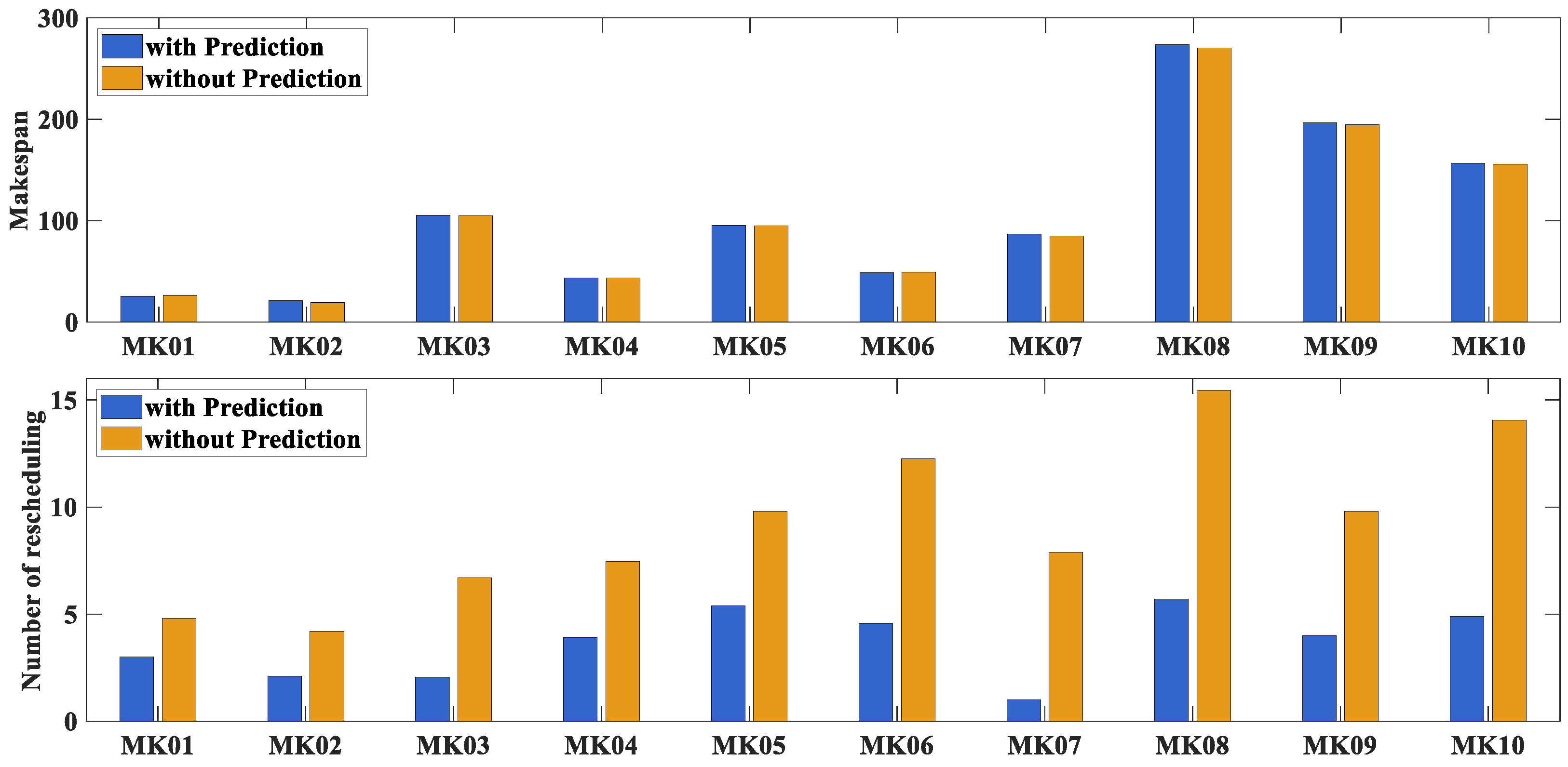
6.5. Performance Evaluation of the Heuristic Scheduling Method

To further validate the effectiveness of the proposed heuristic scheduling method in solving the DDFJSP-VPT, we compare it with two other approaches: the rules-based reactive scheduling method and the hybrid-shift strategy, which comprises left-shift and right-shift strategies. The reactive scheduling method is implemented by applying different rules to factory assignment, machine selection, and operation sequencing; in other words, the combination of three different types of rules is adopted at every scheduling decision point. In this study, we use two factory assignment rules, three machine selection rules, and four operation priority rules, making a total of 24 combinations. Details of the rules are as follows:

Factory Assignment Rule: The first one selects the factory with the fewest unfinished operations for processing. The second selects a factory at random. We refer to them as FAR1 and FAR2, respectively.

Machine Selection Rules: The first selects the machine with the shortest processing time from the available machines. The second selects the machine with the minimum load from the available machines, while the third randomly selects the machine. For convenience, we call them MAR1, MAR2, and MAR3, respectively.

Operation Priority Rules: We employ four prevalent operation priority rules: the shortest processing time (SPT), earliest delivery date (EDD), lowest completion rate (LCR), and random allocation.

The performance of each method is evaluated based on three objectives: the completion time of all jobs, total tardiness, and total factory load, over the entire dynamic scheduling process. Using MK07 as the test instance, each method is independently executed 20 times, with the average value of each objective computed. The results are presented in

Table 7. Comparisons of different dynamic scheduling methods.

Method	Avg Makespan	Avg Tardiness	Avg Factory Load
FAR1 + MAR1 + SPT	152.5570 ± 10.3291	340.3910 ± 40.8320	658.8920 ± 0.3928
FAR1 + MAR2 + SPT	120.6490 ± 8.3210	212.2750 ± 41.7754	771.1400 ± 16.2458
FAR1 + MAR3 + SPT	133.3275 ± 14.4204	348.8570 ± 82.0908	942.0190 ± 42.2810
FAR2 + MAR1 + SPT	149.5850 ± 10.5789	331.1560 ± 63.8415	659.0110 ± 0.4405
FAR2 + MAR2 + SPT	120.3770 ± 12.0717	200.5355 ± 50.2503	764.2850 ± 25.3700
FAR2 + MAR3 + SPT	132.5515 ± 10.5213	332.6000 ± 63.9346	929.0045 ± 22.8944
FAR1 + MAR1 + EDD	141.3315 ± 7.4195	404.9715 ± 52.0484	659.3950 ± 0.6024
FAR1 + MAR2 + EDD	124.3380 ± 12.2159	292.2310 ± 46.5486	775.6655 ± 15.2888
FAR1 + MAR3 + EDD	137.9690 ± 13.8511	429.9040 ± 78.6745	968.0980 ± 38.5276
FAR2 + MAR1 + EDD	145.7560 ± 9.9641	430.5280 ± 48.5627	659.5075 ± 0.6525
FAR2 + MAR2 + EDD	118.6630 ± 9.3815	291.9735 ± 57.8797	776.2800 ± 21.3636
FAR2 + MAR3 + EDD	136.9060 ± 13.6345	416.4960 ± 69.3839	965.7185 ± 43.6098
FAR1 + MAR1 + LCR	131.3435 ± 8.4095	397.8990 ± 38.0280	659.0970 ± 0.6666
FAR1 + MAR2 + LCR	116.6145 ± 7.3871	281.7150 ± 58.0040	778.3695 ± 25.7305
FAR1 + MAR3 + LCR	129.0545 ± 10.2834	404.3545 ± 65.9814	958.8905 ± 32.4785
FAR2 + MAR1 + LCR	133.1555 ± 9.4063	415.0705 ± 77.6714	658.8705 ± 0.6640
FAR2 + MAR2 + LCR	112.7030 ± 8.2004	256.8070 ± 37.8803	793.5140 ± 20.7099
FAR2 + MAR3 + LCR	133.6625 ± 10.9616	434.4575 ± 64.0533	974.2605 ± 35.5795
FAR1 + MAR1 + RAND	124.0835 ± 7.5009	288.9380 ± 49.3850	659.4990 ± 1.0215
FAR1 + MAR2 + RAND	112.8370 ± 11.7223	197.1655 ± 42.9895	784.8950 ± 19.6604
FAR1 + MAR3 + RAND	135.7470 ± 11.9744	392.2830 ± 73.1358	984.9805 ± 39.3767
FAR2 + MAR1 + RAND	121.0080 ± 6.6896	287.0665 ± 54.8079	659.0645 ± 0.6109
FAR2 + MAR2 + RAND	115.0515 ± 10.4489	214.7640 ± 43.8436	785.8260 ± 18.6741
FAR2 + MAR3 + RAND	134.6400 ± 14.9668	392.6080 ± 104.4888	988.4450 ± 48.9537
Hybrid-shift strategy	88.1500 ± 0	50.7400 ± 0	665.9400 ± 0
Proposed scheduling method	83.6725 ± 2.1910	39.5960 ± 11.6871	695.2530 ± 6.8797

.

The results shown in Table 7 clearly demonstrate that our proposed dynamic scheduling method significantly outperforms the other dynamic scheduling methods in terms of reducing the makespan and minimizing tardiness. Additionally, with regard to the total factory load, the combination of the MAR1 rule highlights its superior performance compared to other methods and combination rules. This phenomenon is primarily attributed to the MAR1 rule’s preference for selecting machines with the shortest processing times in terms of task allocation, which effectively reduces the overall factory load. However, this approach may result in an excessive concentration of operations on a limited number of machines, leading to longer waiting times for some machines while leaving others idle. This imbalance may negatively affect the other two objectives. Overall, the proposed scheduling method offers a more efficient solution to dynamic scheduling problems, optimizing both resource utilization and operational performance.

6.6. Further Analysis

In Section 4, the prediction is based on the assumption that processing times satisfy certain constraints with a given probability. As the probability threshold increases, the system’s ability to absorb uncertainty improves, but the scheduling performance may decrease. Therefore, selecting the probability threshold involves a trade-off between uncertainty absorption and scheduling performance. Following [47], a threshold of 0.85 is chosen, and the effectiveness of the proposed prediction strategy is verified through experiments. We compare the initialization scheduling schemes generated with and without the prediction strategy for all test cases. Each scheme is run 20 times, and the average completion time and number of rescheduling events are compared. The results are shown in Figure 11.

As shown in Figure 11, the makespans of the prediction-based and non-prediction-based scheduling methods are nearly identical, while the number of reschedules is reduced in the prediction-based method. Therefore, the proposed prediction method significantly reduces the rescheduling frequency with only a slight compromise in the scheduling performance. This enhancement improves scheduling efficiency and provides a more robust initialization schedule for subsequent dynamic scheduling processes.

7. Conclusions

In this study, a dynamic scheduling model with processing times following a normal distribution is developed for the DDFJSP-VPT. The model simultaneously optimizes three objectives: the makespan, tardiness, and total factory load. A chance-constrained approach is employed to predict the processing times and generate a robust initial scheduling plan. To address the uncertainty and dynamics inherent in production processes, an adaptive heuristic scheduling method is developed, which combines a left-shift adjustment strategy, an insertion-based local adjustment strategy, and the DMOGWO-based global rescheduling strategy. Additionally, for the DMOGWO algorithm, a hybrid initialization scheme is introduced to generate a high-quality initial population. Moreover, the discrete crossover and mutation operations are used to update the wolf pack, enabling the GWO to be effectively applied to discrete combinatorial optimization problems. The experimental results demonstrate the effectiveness of the proposed heuristic schedule method. Furthermore, the utility of the DMOGWO and the prediction scheme is validated. Future studies will focus on exploring more complex dynamic DFJSP problems, particularly those involving multiple dynamic events.

References

1. Luo, C.; Gong, W.; Lu, C. Knowledge-driven two-stage memetic algorithm for energy-efficient flexible job shop scheduling with machine breakdowns. Expert Syst. Appl. 2024, 235, 121149. [Google Scholar] [CrossRef]
2. Zhang, G.; Sun, J.; Liu, X.; Wang, G.; Yang, Y. Solving flexible job shop scheduling problems with transportation time based on improved genetic algorithm. Math. Biosci. Eng. 2019, 16, 1334–1347. [Google Scholar] [CrossRef] [PubMed]
3. Du, B.; Han, S.; Guo, J.; Li, Y. A hybrid estimation of distribution algorithm for solving assembly flexible job shop scheduling in a distributed environment. Eng. Appl. Artif. Intell. 2024, 133, 108491. [Google Scholar] [CrossRef]
4. Wang, L.; Deng, J.; Wang, S.-Y. Survey on optimization algorithms for distributed shop scheduling (Review). Control Decis. 2016, 31, 1–11. [Google Scholar] [CrossRef]
5. Caldeira, R.; Honnungar, S.; Kumar, G.C.M. Feasibility study for converting traditional line assembly into work cells for termination of fiber optics cable. AIP Conf. Proc. 2018, 1943, 020047. [Google Scholar] [CrossRef]
6. Mula, J.; Poler, R.; García-Sabater, J.P.; Lario, F.C. Models for production planning under uncertainty: A review. Int. J. Prod. Econ. 2006, 103, 271–285. [Google Scholar] [CrossRef]
7. Gu, J.; Jiang, T.; Zhu, H.; Zhang, C. Low-Carbon Job Shop Scheduling Problem with Discrete Genetic-Grey Wolf Optimization Algorithm. J. Adv. Manuf. Syst. 2020, 19, 1–14. [Google Scholar] [CrossRef]
8. Luo, S.; Zhang, L.; Fan, Y. Energy-efficient scheduling for multi-objective flexible job shops with variable processing speeds by grey wolf optimization. J. Clean. Prod. 2019, 234, 1365–1384. [Google Scholar] [CrossRef]
9. Zhu, Z.; Zhou, X. An efficient evolutionary grey wolf optimizer for multi-objective flexible job shop scheduling problem with hierarchical job precedence constraints. Comput. Ind. Eng. 2020, 140, 106280. [Google Scholar] [CrossRef]
10. Kong, X.; Yao, Y.; Yang, W.; Yang, Z.; Su, J. Solving the Flexible Job Shop Scheduling Problem Using a Discrete Improved Grey Wolf Optimization Algorithm. Machines 2022, 10, 1100. [Google Scholar] [CrossRef]
11. Komaki, G.M.; Kayvanfar, V. Grey Wolf Optimizer algorithm for the two-stage assembly flow shop scheduling problem with release time. J. Comput. Sci. 2015, 8, 109–120. [Google Scholar] [CrossRef]
12. Zhang, H.; Chen, Y.; Zhang, Y.; Xu, G. Energy-Saving Distributed Flexible Job Shop Scheduling Optimization with Dual Resource Constraints Based on Integrated Q-Learning Multi-Objective Grey Wolf Optimizer. Comput. Model. Eng. 2024, 140, 1459–1483. [Google Scholar] [CrossRef]
13. Li, X.; Xie, J.; Ma, Q.; Gao, L.; Li, P. Improved gray wolf optimizer for distributed flexible job shop scheduling problem. Sci. China Technol. Sci. 2022, 65, 2105–2115. [Google Scholar] [CrossRef]
14. Zhu, K.; Gong, G.; Peng, N.; Zhang, L.; Huang, D.; Luo, Q.; Li, X. Dynamic distributed flexible job-shop scheduling problem considering operation inspection. Expert Syst. Appl. 2023, 224, 119840. [Google Scholar] [CrossRef]
15. Zhu, N.; Gong, G.; Lu, D.; Huang, D.; Peng, N.; Qi, H. An effective reformative memetic algorithm for distributed flexible job-shop scheduling problem with order cancellation. Expert Syst. Appl. 2024, 237, 121205. [Google Scholar] [CrossRef]
16. Zhang, H.; Qin, C.; Xu, G.; Chen, Y.; Gao, Z. An energy-saving distributed flexible job shop scheduling with machine breakdowns. Appl. Soft Comput. 2024, 167, 112276. [Google Scholar] [CrossRef]
17. Chen, Y.; Liao, X.; Chen, G.; Hou, Y. Dynamic Intelligent Scheduling in Low-Carbon Heterogeneous Distributed Flexible Job Shops with Job Insertions and Transfers. Sensors 2024, 24, 2251. [Google Scholar] [CrossRef]
18. Wang, J.; Liu, Y.; Ren, S.; Wang, C.; Wang, W. Evolutionary game based real-time scheduling for energy-efficient distributed and flexible job shop. J. Clean. Prod. 2021, 293, 126093. [Google Scholar] [CrossRef]
19. Lin, C.; Cao, Z.; Zhou, M. Learning-Based Grey Wolf Optimizer for Stochastic Flexible Job Shop Scheduling. IEEE Trans. Autom. Sci. Eng. 2022, 19, 3659–3671. [Google Scholar] [CrossRef]
20. Jin, L.; Zhang, C.; Wen, X.; Sun, C.; Fei, X. A neutrosophic set-based TLBO algorithm for the flexible job-shop scheduling problem with routing flexibility and uncertain processing times. Complex Intell. Syst. 2021, 7, 2833–2853. [Google Scholar] [CrossRef]
21. Caldeira, R.H.; Gnanavelbabu, A. A simheuristic approach for the flexible job shop scheduling problem with stochastic processing times. Simulation 2020, 97, 215–236. [Google Scholar] [CrossRef]
22. Sun, L.; Lin, L.; Li, H.; Gen, M. Cooperative Co-Evolution Algorithm with an MRF-Based Decomposition Strategy for Stochastic Flexible Job Shop Scheduling. Mathematics 2019, 7, 318. [Google Scholar] [CrossRef]
23. Mokhtari, H.; Dadgar, M. Scheduling optimization of a stochastic flexible job-shop system with time-varying machine failure rate. Comput. Oper. Res. 2015, 61, 31–45. [Google Scholar] [CrossRef]
24. Shahgholi Zadeh, M.; Katebi, Y.; Doniavi, A. A heuristic model for dynamic flexible job shop scheduling problem considering variable processing times. Int. J. Prod. Res. 2018, 57, 3020–3035. [Google Scholar] [CrossRef]
25. Zhong, X.; Han, Y.; Yao, X.; Gong, D.; Sun, Y. An evolutionary algorithm for the multi-objective flexible job shop scheduling problem with uncertain processing time. Sci. Sin. Inform. 2023, 53, 737–757. [Google Scholar] [CrossRef]
26. Zhang, L.; Feng, Y.; Xiao, Q.; Xu, Y.; Li, D.; Yang, D.; Yang, Z. Deep reinforcement learning for dynamic flexible job shop scheduling problem considering variable processing times. J. Manuf. Syst. 2023, 71, 257–273. [Google Scholar] [CrossRef]
27. Fu, Y.; Gao, K.; Wang, L.; Huang, M.; Liang, Y.-C.; Dong, H. Scheduling stochastic distributed flexible job shops using an multi-objective evolutionary algorithm with simulation evaluation. Int. J. Prod. Res. 2024, 63, 86–103. [Google Scholar] [CrossRef]
28. Charnes, A.; Cooper, W.W. Chance-Constrained Programming. Manage. Sci. 1959, 6, 73–79. [Google Scholar] [CrossRef]
29. Muralidhar, K.; Swenseth, S.R.; Wilson, R.I. Describing processing time when simulating JIT environments. Int. J. Prod. Res. 1992, 30, 1. [Google Scholar] [CrossRef]
30. Chang, P.; Chen, S.; Lin, K. Two-phase sub population genetic algorithm for parallel machine-scheduling problem. Expert Syst. Appl. 2005, 29, 705–712. [Google Scholar] [CrossRef]
31. Bitar, A.; Dauze’re-Pe’re’s, S.; Yugma, C.; Roussel, R. A memetic algorithm to solve an unrelated parallel machine scheduling problem with auxiliary resources in semiconductor manufacturing. J. Sched. 2016, 19, 367–376. [Google Scholar] [CrossRef]
32. He, W.; Sun, D.-h. Scheduling flexible job shop problem subject to machine breakdown with route changing and right-shift strategies. Int. J. Adv. Manuf. Technol. 2012, 66, 501–514. [Google Scholar] [CrossRef]
33. Deb, K.; Pratap, A.; Agarwal, S.; Meyarivan, T. A fast and elitist multiobjective genetic algorithm: NSGA-II. IEEE Trans. Evol. Comput. 2002, 6, 182–197. [Google Scholar] [CrossRef]
34. Gao, K.Z.; Suganthan, P.N.; Pan, Q.K.; Chua, T.J.; Cai, T.X.; Chong, C.S. Pareto-based grouping discrete harmony search algorithm for multi-objective flexible job shop scheduling. Inf. Sci. 2014, 289, 76–90. [Google Scholar] [CrossRef]
35. Lu, C.; Gao, L.; Li, X.; Xiao, S. A hybrid multi-objective grey wolf optimizer for dynamic scheduling in a real-world welding industry. Eng. Appl. Artif. Intell. 2017, 57, 61–79. [Google Scholar] [CrossRef]
36. Wang, X.; Gao, L.; Zhang, C.; Shao, X. A multi-objective genetic algorithm based on immune and entropy principle for flexible job-shop scheduling problem. Int. J. Adv. Manuf. Technol. 2010, 51, 757–767. [Google Scholar] [CrossRef]
37. Wang, L.; Zhou, G.; Xu, Y.; Liu, M. An enhanced Pareto-based artificial bee colony algorithm for the multi-objective flexible job-shop scheduling. Int. J. Adv. Manuf. Technol. 2012, 60, 1111–1123. [Google Scholar] [CrossRef]
38. Brandimarte, P. Routing and scheduling in a flexible job shop by tabu search. Ann. Oper. Res. 1993, 41, 157–183. [Google Scholar] [CrossRef]
39. Zitzler, E.; Thiele, L. Multiobjective evolutionary algorithms: A comparative case study and the strength Pareto approach. IEEE Trans. Evol. Comput. 1999, 3, 257–271. [Google Scholar] [CrossRef]
40. Zitzler, E.; Thiele, L.; Laumanns, M.; Fonseca, C.M.; Da Fonseca, V.G. Performance assessment of multiobjective optimizers: An analysis and review. IEEE Trans. Evol. Comput. 2003, 7, 117–132. [Google Scholar] [CrossRef]
41. Tang, J.; Gong, G.; Peng, N.; Zhu, K.; Huang, D.; Luo, Q. An effective memetic algorithm for distributed flexible job shop scheduling problem considering integrated sequencing flexibility. Expert Syst. Appl. 2024, 242, 122734. [Google Scholar] [CrossRef]
42. Qingfu, Z.; Hui, L. MOEA/D: A Multiobjective Evolutionary Algorithm Based on Decomposition. IEEE Trans. Evol. Comput. 2007, 11, 712–731. [Google Scholar] [CrossRef]
43. Zitzler, E.; Laumanns, M.; Thiele, L. SPEA2: Improving the Strength Pareto Evolutionary Algorithm for Multiobjective Optimization; Technical Report Gloriastrasse; 103, TIK-Rep; Swiss Federal Institute of Technology: Lausanne, Switzerland, 2001; pp. 1–20. [Google Scholar] [CrossRef]
44. Demšar, J. Statistical comparisons of classifiers over multiple data sets. J. Mach. Learn. Res. 2006, 7, 1–30. [Google Scholar]
45. Shen, X.-N.; Yao, X. Mathematical modeling and multi-objective evolutionary algorithms applied to dynamic flexible job shop scheduling problems. Inf. Sci. 2015, 298, 198–224. [Google Scholar] [CrossRef]
46. Bader, J.; Zitzler, E. HypE: An Algorithm for Fast Hypervolume-Based Many-Objective Optimization. Evol. Comput. 2011, 19, 45–76. [Google Scholar] [CrossRef] [PubMed]
47. Chuanjun, Z.; Wen, Q.; Mengzhou, Z.; Guang, C.; Chaoyong, Z. Multi-objective flexible job shops robust scheduling problem under stochastic processing times. China Mech. Eng. 2016, 27, 1667–1672. [Google Scholar] [CrossRef]
Figure 1. Flowchart of the proposed heuristic scheduling method in the DDFJSP-VPT.
Applsci 15 02281 g001
Figure 2. Illustration of the local adjustment strategy.
Applsci 15 02281 g002
Figure 3. Binary tree of subsequent operations.
Applsci 15 02281 g003
Figure 4. Illustration of the Three-Layer Encoding Scheme.
Applsci 15 02281 g004
Figure 5. Illustration of the decoded schedule of the chromosome shown in Figure 4.
Applsci 15 02281 g005
Figure 6. Illustration of the crossover for OS and MS.
Applsci 15 02281 g006
Figure 7. Illustration of the mutation for OS and MS.
Applsci 15 02281 g007
Figure 8. Performance evaluation with varying N values.
Applsci 15 02281 g008
Figure 9. Performance scores of four algorithms across all rescheduling points.
Applsci 15 02281 g009
Figure 10. Average performance scores of four algorithms across all rescheduling points.
Applsci 15 02281 g010
Figure 11. Comparison of the dynamic scheduling method with and without predictions.
Applsci 15 02281 g011