Impact of Non-Landslide Sample Sampling Strategies and Model Selection on Landslide Susceptibility Mapping

Abstract

This study investigated the influence of non-landslide sampling strategies on landslide susceptibility assessment (LSA) performance and explored approaches to minimizing uncertainty in model selection. Five non-landslide sampling strategies were evaluated using the random forest (RF) model to generate landslide susceptibility maps (LSMs) for each scenario. To assess the impact of these strategies, this study employed a receiver operating characteristic (ROC) curve, a confusion matrix, and various statistical indicators. Additionally, the mean susceptibility indices derived from the gradient boosting decision tree (GBDT), support vector machine (SVM), and RF models were analyzed to evaluate their effectiveness in reducing the uncertainty during model selection. The GBDT, SVM, and RF were selected for their ability to handle complex, nonlinear relationships in the data, superior generalization capability, effective mitigation of overfitting risks, high predictive performance, and robustness. The findings revealed that selecting non-landslide samples from slope units without landslides enhances accuracy and averaging across models mitigated the uncertainty associated with landslide susceptibility models. Furthermore, this study demonstrated that the non-landslide sample selection method significantly improved prediction accuracy, particularly when samples were drawn from very-low-susceptibility zones identified by pre-classified machine learning models. These results highlight the importance of refining sample selection strategies and integrating multiple machine learning models to improve the reliability and accuracy of landslide susceptibility assessments. This approach provides valuable insights for future research and practical applications in risk mitigation and disaster management by offering a more precise depiction of low-susceptibility areas, thereby reducing the occurrence of false positives in landslide prediction.

1. Introduction

Landslides are among the most widespread and destructive geological disasters worldwide [1]. Landslide susceptibility assessment (LSA) and landslide susceptibility mapping (LSM) are effective tools for identifying landslide-prone areas and supporting risk management efforts [2]. The regional LSA evaluates the likelihood of landslide occurrence within a specific area based on local topographical conditions [3], providing predictions on where landslides are most likely to occur [4].

In recent years, the rapid development of 3S technologies (GIS, RS, and GPS) has led to their extensive application in landslide spatial prediction. The advanced processing capabilities of remote sensing images and robust spatial analysis functions of GIS have significantly enhanced landslide spatial prediction [5]. Currently, landslide spatial prediction relies predominantly on GIS platforms to perform susceptibility assessments through multi-factor correlation analysis. Various models have been developed, including physical [6], traditional statistical [7], and machine learning models [2,8,9]. Among these, machine learning models have become a research focus because of their ability to overcome the limitations of traditional statistical methods, such as the need for predefined assumptions. Unlike traditional methods, machine learning models do not require input variables to follow a normal distribution and effectively capture nonlinear relationships between environmental factors and landslide susceptibility. These models are particularly adept at fitting highly nonlinear relationships. Commonly employed machine learning models include logistic regression, k-nearest neighbor, support vector machines, extremely randomized trees, Bayesian networks, artificial neural networks, gradient boosting decision trees, and random forests. For example, Liu et al. [10] applied a logistic regression model to assess landslide susceptibility in the Wuling Mountains and demonstrated its strong accuracy in predicting landslide-prone areas. Jafari et al. [11] employed the k-nearest neighbor algorithm to evaluate landslide susceptibility in Southwestern China, showing that the model effectively handled landslide data in complex topographic conditions. Li et al. [12] combined support vector machines (SVMs) with geological and topographic factors, revealing that the SVM approach significantly improved prediction accuracy in complex geological environments while efficiently processing high-dimensional data. Zhang et al. [13] applied the extremely randomized trees model for landslide susceptibility assessment in the Qinling Mountains, highlighting its enhanced stability and accuracy under intricate geological conditions. Zhou et al. [14] implemented a Bayesian network model in the Sichuan Basin, demonstrating its effectiveness in handling various uncertainties related to landslide occurrence. Xu et al. [15] applied artificial neural networks (ANNs) for landslide susceptibility modeling in the Loess Plateau, showing that ANNs effectively captured nonlinear relationships in landslide-prone areas, improving prediction accuracy. Wang et al. [16] employed gradient boosting decision trees (GBDTs) in the Three Gorges Reservoir area, finding that GBDTs enhanced prediction accuracy through the integration of multiple weak classifiers while effectively addressing variable geological conditions. Zhang et al. [17] applied random forest models to assess landslide susceptibility in the Tibetan Plateau, demonstrating their capability to handle high-dimensional data, identify key factors influencing landslides and provide efficient predictive results.

Despite these advancements, significant uncertainties persist in the application of machine learning models for the spatial prediction of landslides, particularly concerning the selection of LSA models and data sampling. The suitability of LSA models varies across research areas, leading to considerable variability in results among researchers using different models. This variability makes discrepancies in LSA outcomes evident and hinders identification of the model with the best predictive performance, thereby limiting the application and promotion of LSA findings. Consequently, improving the applicability and generalization of machine learning models in regional LSA remains a critical area for further research [18].

Non-landslide samples serve as target label data for landslide susceptibility modeling and play a crucial role in determining the applicability of susceptibility models. Thus, careful and rational selection of non-landslide samples is essential for enhancing the accuracy of LSA. The current literature identifies three primary methods for selecting non-landslide samples: (1) buffering outward from the edges of landslides to generate sample data [19,20]; (2) randomly selecting samples from non-landslide areas [21,22]; and (3) selecting samples from regions with gentle slopes that do not experience landslides [23,24]. However, these methods involve varying degrees of subjectivity and are influenced by the characteristics of specific factors, thereby introducing uncertainties into the selection of non-landslide samples. These challenges hinder the accurate prediction of landslide susceptibility, making this a critical and active area of research.

Badong County, located at the heart of the Three Gorges Reservoir area, is highly susceptible to landslide-induced geological hazards. Among the regions within the Three Gorges Reservoir, Badong County has experienced a particularly high frequency of landslides. Since the impoundment of reservoirs, fluctuations in water levels and associated issues such as reservoir bank landslides have attracted significant attention. Notably, during periods of high water levels, landslide occurrence increases, posing substantial risks to local infrastructure, public safety, and the ecological environment. This study addressed the critical need for disaster prevention and mitigation by conducting a regional landslide susceptibility assessment. Effective strategies were explored to minimize uncertainties related to non-landslide sample selection and model choice, with the aim of producing more accurate and reliable landslide susceptibility zoning results. These findings will serve as a solid foundation and valuable reference for future disaster prevention, mitigation efforts, and regional landslide risk assessment. This study addressed the uncertainties in landslide susceptibility modeling by proposing the application of average susceptibility indices from multiple models as the final susceptibility index to reduce uncertainty in model selection. To minimize the uncertainty in non-landslide sample selection, the non-landslide samples were derived from slope units without landslides, thereby avoiding similarities in the disaster-causing factors and environmental conditions associated with selecting the samples from slope units containing landslides. Non-landslide samples were also selected beyond an 800 m buffer zone around landslide points, with the buffer distance based on the largest recorded landslide in the study area, which measured 1600 m in length and 1300 m in width. This method was compared with the approach of selecting non-landslide samples in slope units without landslides. Additionally, non-landslide samples were selected from very-low-susceptibility areas identified by the LR, SVM, and GBDT models to analyze the effects of different sampling strategies on LSM.

2. Materials

2.1. Study Area

Badong County (Figure 1) is situated in the southwestern part of Hubei Province, in the upper and middle reaches of the Yangtze River, northeast of Enshi Tujia and Miao Autonomous Prefecture. The topography of the study area features higher elevations in the northwest, gradually lowering toward the southeast, and is classified as an erosion-structural landscape. The prominent landforms include high, medium, and low mountains, with the highest elevation reaching 2977 m and a maximum height difference of 3008 m. The region falls within a subtropical monsoon climate zone characterized by warm average temperatures, abundant rainfall, and distinct seasonal variations. The average temperature is 17.5 °C, while rainfall averages 1285.9 mm annually, most occurring during the flood season between April and September. The area has a dense river network dominated by the Yangtze and Qingjiang Rivers. The exposed strata in the region primarily consist of Permian and Lower Triassic Jialingjiang Group carbonate rocks, along with Middle Triassic Badong Group carbonate rocks interbedded with clastic rocks. As of 2020, the Hubei Provincial Environmental Monitoring Station reported 642 geological disaster incidents in Badong County, including 548 landslides (79 classified as unstable slopes), 80 collapses, 10 ground subsidence events, and 4 debris flows.

2.2. Data Source and Preparation of Influencing Factors

2.2.1. Data Source

(1) Digital Elevation Model (DEM) data: These data were used to extract various topographic factors, including slope, aspect, curvature, topographic wetness index (TWI), flow path length, and flow width. The data were sourced from the Geospatial Data Cloud website (http://www.gscloud.cn/ (accessed on 12-July-2024)) with a spatial resolution of 30 m. For example, Liu et al. [25] extracted topographic features such as slope, aspect, and curvature from DEM data and used machine learning models to generate landslide susceptibility maps. Their findings highlight the effectiveness of DEM data in predicting landslide-prone areas.

(2) Basic geological data: Geological data were used to analyze the engineering geological rock group (EGRG) distribution and slope structure in the study area. The data were sourced from the National 1:200,000 Digital Geological Map (Public Edition) spatial database provided by the Geological Science Data Publishing System (http://dcc.ngac.org.cn/cn/page/index (accessed on 12-July-2024)). For example, Wang et al. [26] investigated the significance of geological data, particularly EGRG, in understanding regional landslide behavior. They used geological map data to analyze landslide distribution and incorporated it into landslide susceptibility modeling.

(3) Rainfall stations and rainfall data: These data, provided by the China Geological Survey, were used to analyze the relationship between rainfall and landslide occurrence in the study area and to calculate the mean annual rainfall. For example, Wang et al. [27] utilized Kriging interpolation to estimate the annual rainfall distribution in the Xijiang River Basin and found that incorporating spatially distributed rainfall data significantly improved the accuracy of landslide susceptibility assessments. Their study emphasizes the importance of considering rainfall distribution in landslide hazard modeling.

(4) Land use data and normalized difference vegetation index (NDVI): These data were sourced from the United States Geological Survey (earthexplorer.usgs.gov (accessed on 18-July-2024)) and Landsat-8 imagery. For example, Yang et al. [28] used Landsat-8 imagery to extract NDVI values and assess the role of vegetation in mitigating or exacerbating landslide risks. Similarly, Zhao et al. [29] incorporated NDVI and land use data to examine the influence of different land cover types on landslide occurrence and proposed land use planning strategies to reduce landslide risks.

(5) Vector data: This included information on administrative boundaries, national water systems, road networks, and other relevant features sourced from the National Geographic Information Resources Catalogue Service System (https://www.webmap.cn/ (accessed on 12-July-2024)).

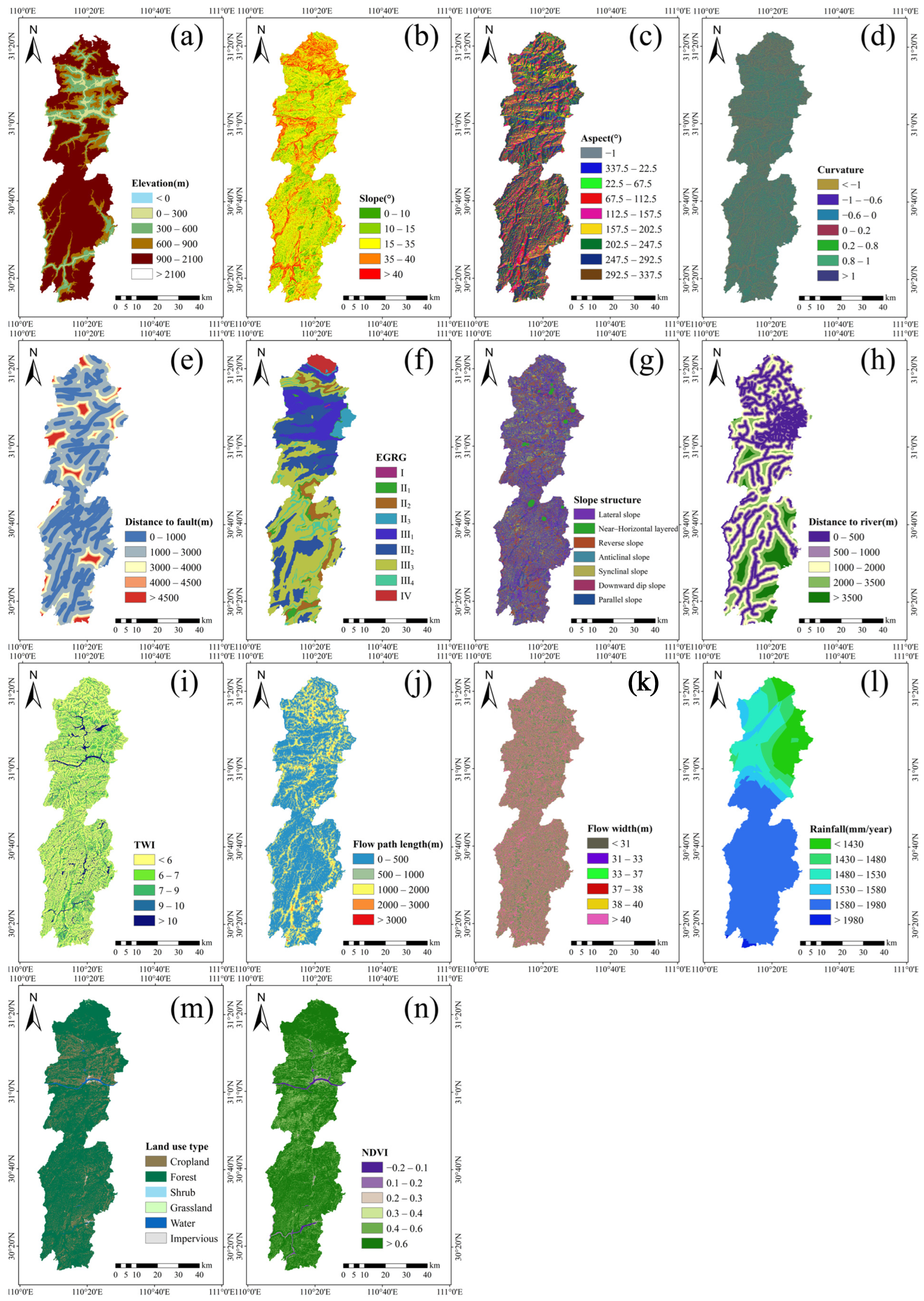
2.2.2. Influencing Factors

Considering the geological conditions, geographic environment, and characteristics of landslide disasters in Badong County, a 30 m × 30 m raster was selected as the basic unit for spatial landslide prediction in accordance with the technical requirements of the China Geological Survey’s geological disaster investigations (1:50,000). Based on prior research, this study utilized ArcGIS version 10.7 to extract 14 influencing factor layers (Figure 2) as indicators for modeling landslide susceptibility in the study area. These factors included four topographic-geomorphic variables (elevation, slope, aspect, and curvature), three geological condition variables (distance from fault, EGRG, and slope structure), five hydrological condition variables (distance to river, TWI, flow path length, flow width, and mean annual rainfall in 2020), and two surface cover variables (land use type and NDVI).

In accordance with the “1:50,000 Engineering Geological Survey Specifications” and considering the geological characteristics of the study area, such as rock type, structure, and strength, the region was classified into nine engineering geological rock groups (

Table 1. Classification of EGRG based on geotechnical characteristics.

Construction Type	Lithological Unit Code	Lithological Unit Name
Loose soils	I	Quaternary loose soils
Clastic rock	II1	Rock formation dominated by hard, thick-bedded sandstone
	II2	Rock formation dominated by weak, layered claystone
	II3	Alternating hard and soft layered sandstone and claystone interbedded formation
Carbonate rock	III1	Slightly karstified alternating soft and hard layered clastic rock with carbonate interbedding formation
	III2	Highly karstified hard-layered carbonate rock formation
	III3	Moderately karstified alternating soft and hard layered carbonate rock with clastic interbedding formation
	III4	Moderately karstified alternating soft and hard layered carbonate and clastic rock interbedded formation
Metamorphic rock	IV	Migmatite and gneiss formation

).

The slope structure in this study was classified based on the relationship between stratigraphic inclination, dip slope gradient, and direction, with the specific classification criteria presented in

Table 2. Slope structure classification criteria.

Category	Types of Slope Structures	Definition
1	Downward dip slope	((|α − β|∈(0, 30°]) or (|α − β|∈[330°, 360°))) and (γ > 10°) and (δ > γ)
2	Synclinal slope	((|α − β|∈(0, 30°]) or (|α − β|∈[330°, 360°))) and (γ > 10°) and (δ < γ)
3	Parallel slope	(|α − β|∈(30°, 60°]) or (|α − β|∈[300°, 330°))
4	Lateral slope	(|α − β|∈(60°, 120°]) or (|α − β|∈[240°, 300°))
5	Anticlinal slope	(|α − β|∈(120°, 150°]) or (|α − β|∈[210°, 240°))
6	Reverse slope	(|α − β|∈(150°, 180°]) or (|α − β|∈[180°, 210°))

Where α is the slope direction, β is the rock inclination, γ is the rock dip, and δ is the slope gradient.

.

3. Methodologies

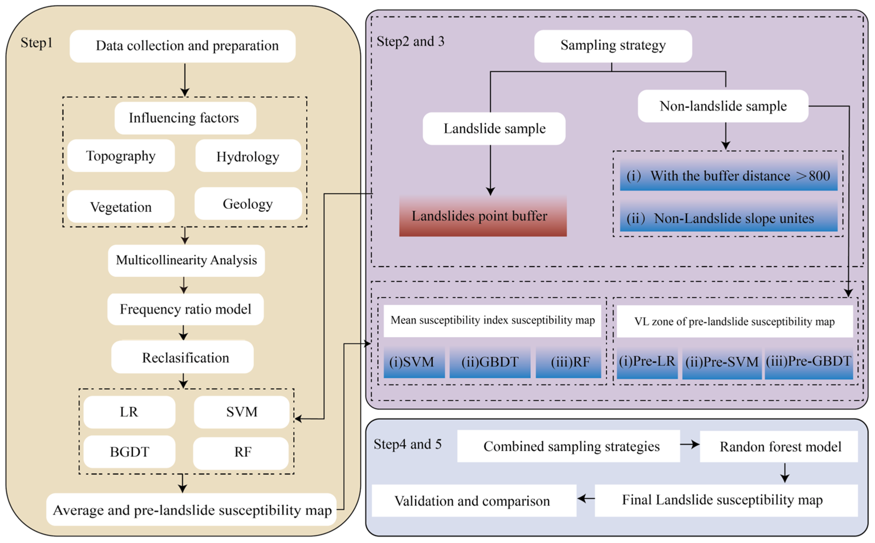
3.1. Modelling Procedure

The flowchart of this study, shown in Figure 3, outlines five key stages. In the first stage, data preparation and factor reclassification, all the influencing factors were converted into 30 m-resolution raster data using ArcGIS. The frequency ratios (FRs) for continuous factors were calculated using smaller intervals, and subcategories with similar FR values were grouped to establish factor classifications.

For the sampling strategy of landslide and non-landslide data in the second stage, landslide samples were generated by buffering around landslide points, with the buffer radius determined by the area of each landslide. Buffered areas within slope units containing landslides were retained, whereas those within slope units without landslides were excluded. Non-landslide samples were identified using five distinct methods. In the “Slope” dataset, samples were selected from slope units without landslides. In the “Buffer” dataset, samples were extracted from areas outside an 800 m buffer around landslide points, the buffer distance based on the largest recorded landslide in the study area, which measured 1600 m in length and 1300 m in width; and the non-landslide samples were extracted from the zones of very low susceptibility identified by the LR, SVM, and GBDT models, forming the “Pre-LR”, “Pre-SVM”, and “Pre-GBDT” datasets, respectively.

In the third stage, the average method to reduce model selection uncertainty refers to averaging the susceptibility indices from different models to mitigate the uncertainty in the model selection process.

For the LSM in the fourth stage, the LSM performance of the LR, SVM, GBDT, and RF models was compared using the “Buffer” and “Slope” datasets through combining the aforementioned landslide and non-landslide sampling strategies. Additionally, the RF model was applied to compare LSM performance across the “Pre-LR”, “Pre-SVM”, and “Pre-GBDT” datasets.

For the validation and comparison process in the fifth stage, the receiver operating characteristic (ROC) curves and area under the curve (AUC) values for each scenario were calculated to assess model performance and evaluate the impact of different sampling strategies on LSA. A confusion matrix of the model was generated and exported. Furthermore, the distribution and proportion of existing landslide points within each susceptibility zone were recorded, along with the distribution and proportion of pixels for each susceptibility zone.

3.2. Frequency Ratio Analysis

The FR reflects the significance of different attribute intervals of the indicator factors in relation to landslide susceptibility. An FR greater than 1 indicates that a specific category interval influences landslide occurrence, whereas an FR less than 1 suggests no association with landslide formation [30]. In this study, the FR method was applied to categorize continuous indicator factors, and the FR for each influencing factor category was calculated using the following formula:

$$FR={\displaystyle \frac{\frac{A}{B}}{\frac{C}{D}}},$$

(1)

where $A$ is the landslide area within a specific category, $B$ is the total landslide area in the study region, $C$ is the area occupied by that category in the study region, and $D$ is the total area of the study region.

Continuous factors were segmented into smaller intervals, and the frequency ratios for both continuous and categorical factors were computed using the above formula. The intervals of the continuous factors with similar frequency ratios were subsequently combined. The results are presented in

Table 3. Classification criteria for influencing factors based on FRs.

Influencing Factors	Classification	FR	Influencing Factors	Classification	FR
Aspect (°)	Plane	0.00	EGRG	I	0.00
	North	1.27		II1	1.61
	Northeast	1.10		II2	0.94
	East	1.26		II3	0.53
	Southeast	1.02		III1	3.98
	South	0.98		III2	0.19
	Southwest	0.64		III3	0.67
	West	0.78		III4	1.55
	West	0.96		IV	0.00
Slope structure	Near-horizontal layered	0.76	Curvature	<−1	0.88
	Downward dip slope	1.07		−1–−0.6	1.04
	Synclinal slope	0.94		−0.6–0	1.14
	Parallel slope	0.93		0–0.2	1.20
	Lateral slope	0.89		0.2–0.8	1.14
	Anticlinal slope	1.05		0.8–1	1.04
	Reverse slope	1.30		>1	0.87
Elevation (m)	<0	0.00	Land use type	Cropland	2.31
	0–300	5.98		Forest	0.64
	300–600	2.81		Shrub	0.36
	600–900	1.19		Grassland	0.37
	900–2100	0.30		Water	0.00
	>2100	0.00		Impervious	11.02
Flow width (m)	<31	1.05	Rainfall (mm/year)	<1430	0.00
	31–33	1.13		1430–1480	2.57
	33–37	1.06		1480–1530	0.97
	37–38	1.01		1530–1580	1.39
	38–40	1.04		1580–1980	0.67
NDVI	−0.2–0.1	0.10	TWI	<6	0.69
	0.1–0.2	2.59		6–7	1.28
	0.2–0.3	6.05		7–9	1.69
	0.3–0.4	2.65		9–10	1.64
	0.4–0.6	1.58		>10	0.89
Distance to river (m)	0–500	1.73	Distance to fault (m)	0–1000	1.10
	500–1000	1.30		1000–3000	0.84
	1000–2000	0.56		3000–4000	1.44
	2000–3500	0.17		4000–4500	1.02
	>3500	0.03		>4500	0.73
Slope (°)	0–10	0.69	Flow path length (m)	0–500	0.46
	10–15	0.97		500–1000	1.32
	15–35	1.14		1000–2000	2.60
	35–40	0.92		2000–3000	1.89
	>45	0.67		>3000	0.00

.

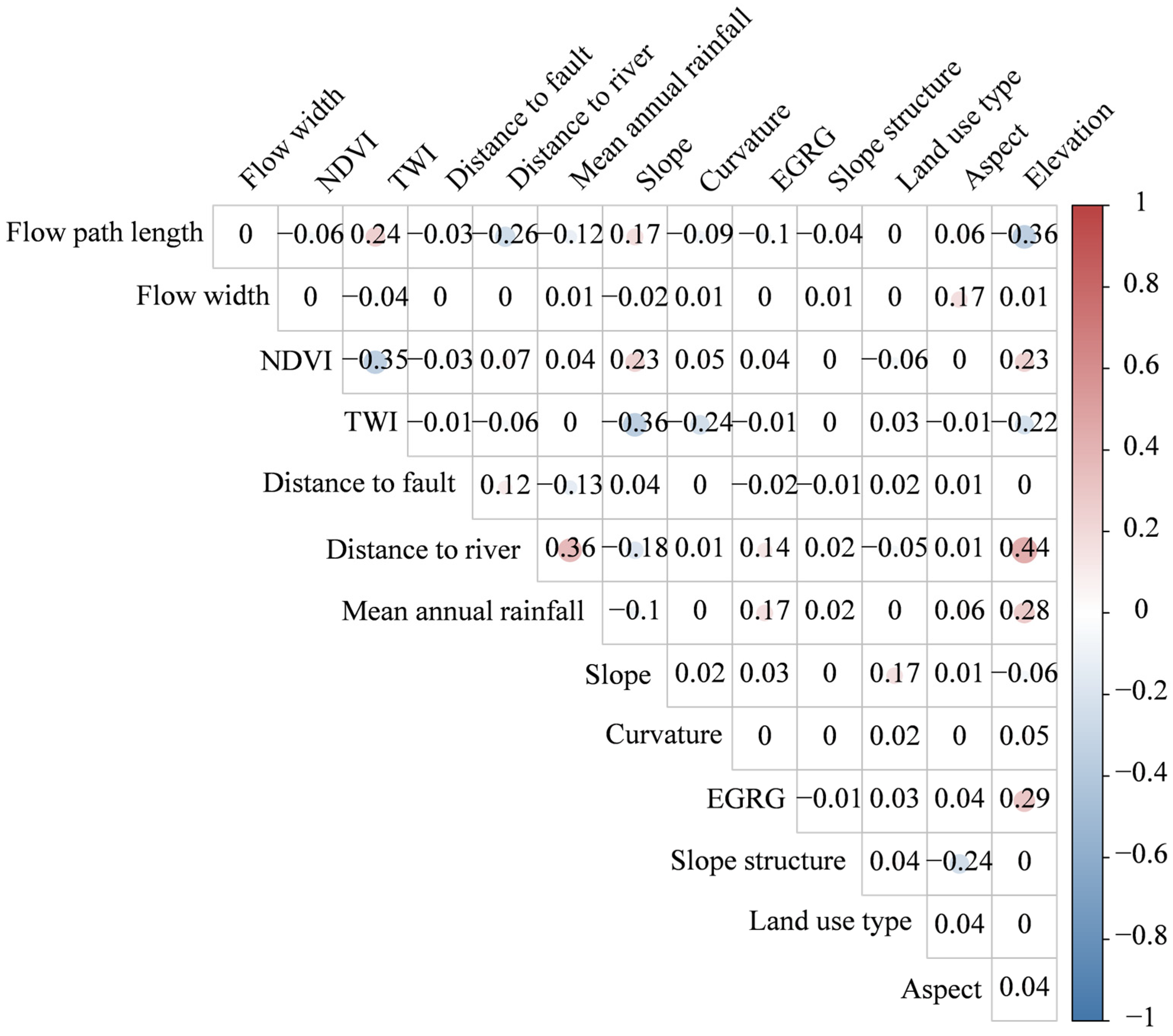
3.3. Multicollinearity Analysis

To construct a susceptibility assessment index system, several factors related to the occurrence and development of geological disasters were selected. However, these factors are not entirely independent and may exhibit some degree of correlation. If not properly addressed, overlapping influence weights among the indicator factors can lead to errors or inaccuracies in assessment results. Therefore, it is crucial to filter the factors during selection to ensure their independence while maintaining the accuracy of the input parameters. To avoid interference and overlap, factors with a minimal influence on landslide susceptibility or overlapping weights should be eliminated. This study utilized the Pearson correlation coefficient method to analyze the correlations between influencing factors.

The method proposed by the statistician Karl Pearson [31] quantifies the correlation between factors using the correlation coefficient r. The primary objective was to describe differences in the target variables. The closer the absolute value of r is to 1, the greater the correlation between the factors. The Pearson correlation coefficient is a commonly used metric that can be calculated by dividing the covariance of two factors by the product of their standard deviations, as shown in Equation (2):

$$r_{\left(X,Y\right)}={\displaystyle \frac{Cov\left(\left(X,Y\right)\right)}{\sqrt{Var\left[X\right]Var\left[Y\right]}}},$$

(2)

where $Var\left[X\right]$ represents the variance of $X$, $Var\left[Y\right]$ represents the variance of $Y$, and $Cov\left(\left(X,Y\right)\right)$ is the covariance between $X$ and $Y$.

The influencing factor data were imported into the SPSS statistical analysis software, where the “Bivariate” tool was adopted for analysis. The correlation coefficients between the influencing factors are shown in Figure 4. A high correlation coefficient (0.44) was identified between elevation and distance to rivers, leading to the exclusion of the elevation factor from this study.

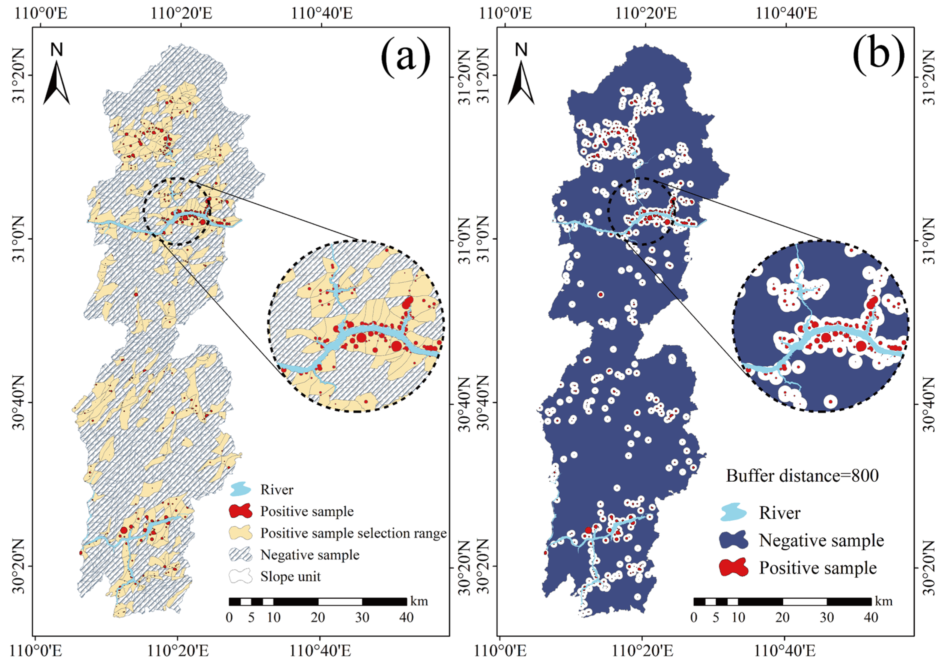
3.4. Assessment Unit and Sample Selection

This study involved multiple factor categories, with the data presented in a raster format that was regular in shape and convenient for computation. Using slope units as assessment units requires the extraction of statistical metrics for each factor, thereby significantly increasing workload and potentially introducing errors. By selecting appropriately sized raster units, the uncertainty is reduced while meeting accuracy requirements. In this study, raster units with a resolution of 30 m × 30 m were selected as assessment and mapping units. Statistical analysis revealed that the study area contained 3,721,512 raster cells.

The landslide catalog data comprise point data, which may have spatial resolution inconsistencies, posing challenges in accurately representing the areal characteristics of landslides. To address this, a buffering method was implemented to align landslide morphology more closely. Buffers were created around the landslide points and extended outward, based on the landslide area. Buffered areas within slope units containing landslides were retained, whereas those within slope units without landslides were excluded. Non-landslide samples were selected using five methods. The samples were selected from the slope units without landslides to form the “Slope” dataset (Figure 5a). An 800 m-radius buffer was established around landslide points, and the samples from outside this buffer formed the “Buffer” dataset (Figure 5b). The buffer distance was determined based on the largest recorded landslide in the study area, which was 1600 m in length and 1300 m in width. Additionally, the non-landslide samples were selected from very-low-susceptibility zones identified by the LR, SVM, and GBDT models, resulting in the “Pre-LR”, “Pre-SVM”, and “Pre-GBDT” datasets, respectively.

3.5. Machine Learning Models

3.5.1. Logistic Regression

Logistic regression (LR) [32] is a multivariate regression model that utilizes multiple independent variables to predict a single dependent variable, making it a widely adopted method for the spatial prediction of geological disasters. The core principle of LR is to transform domain values from negative to positive infinity into a probability range between 0 and 1. Values closer to 0 represent one class, whereas values closer to 1 represent another, indicating the non-occurrence and occurrence of geological disaster events, respectively. This transformation is achieved using the sigmoid function:

$$g\left(z\right)={\displaystyle \frac{1}{1+e^{-z}}},$$

(3)

where $g\left(z\right)$ represents the estimated probability of the occurrence of geological disasters, varying from 0 to 1 along an S-shaped curve; and $z$ is a linear combination:

$$z=b_0+b_1{x}_1+b_2{x}_2+\dots +b_n{x}_n,$$

(4)

where $x_1,x_2,\dots \dots ,x_n$ represent the independent variables that influence the occurrence of geological disasters; and $b_0,b_1,\dots \dots ,b_n$ denote the regression coefficients associated with these variables.

3.5.2. Gradient Boosting Decision Tree

The gradient boosting decision tree (GBDT) [33] is an optimization algorithm known for its strong generalization performance on real-world distributions. It is widely applied to classification and regression tasks by employing regularization functions to enhance training outcomes and mitigate overfitting. The GBDT operates through multiple iterations of weak classifiers, which are weighted and aggregated at each step to produce the final classification result. The GBDT model is ultimately described as:

$$F_m={\sum }_{m=1}^M\begin{array}{c}T\left(x,{\theta }_m\right)\end{array},$$

(5)

where $M$ is the number of iterations, $T\left(x,{\theta }_m\right)$ represents the weak classifier generated in the $m$-th iteration, and ${\theta }_m$ is the loss function:

$${\theta }_m=argmin{\sum }_{i=1}^{N}L\left(y_i,F_{m-1}\left(x_i\right)+T\left(x_i,{\theta }_m\right)\right),$$

(6)

where $y_i$ represents the true label of the i-th sample, $F_{m-1}\left(x_i\right)$ is the model’s prediction for the $i$-th sample after the $m-1$-th iteration, and $T\left(x_i,{\theta }_m\right)$ is the output of the weak classifier generated in the m-th iteration with parameters ${\theta }_m$. Function $L$ denotes the loss function and quantifies the error between predicted values and actual labels. The objective is to determine the parameters ${\theta }_m$ that minimize total loss across all $N$ samples in the dataset.

In the current iteration $F_{m-1}\left(x_i\right)$, the GBDT algorithm determines the parameters of the next classifier by minimizing ${\theta }_m$. During each learning step, the algorithm aims to minimize the loss function, striving for either local or global optimality. The GBDT is a flexible and robust method suitable for both classification and prediction tasks.

3.5.3. Support Vector Machine

A support vector machine (SVM) is a non-parametric supervised machine learning algorithm designed to address nonlinear classification and regression problems using mathematical tools. The SVM is grounded in the statistical learning theory developed by Cortes and Vapnik [34]. It achieves its desired output by transforming input data into a high-dimensional space using kernel functions and subsequently mapping the results back to a two-dimensional space [35]. This algorithm is particularly suitable for binary classification problems involving both positive and negative landslide samples. In such cases, the SVM seeks to identify the optimal separating hyperplane in the feature space that maximizes the margin between the two classes.

Spatial prediction of geological disasters is a binary classification problem, where outcomes are categorized as either “present” or “absent”. The core principle of the SVM lies in identifying a hyperplane within the training dataset that separates the two classes while maximizing the margin between them. The hyperplane is mathematically represented as:

$$W^{T}x+b=0,$$

(7)

where $W$ is the normal vector that determines the orientation of the hyperplane, $x$ is the input feature vector, and $b$ is the bias term controlling the offset of the hyperplane from the origin. This boundary partitions the feature space, enabling the classification of data points.

The hyperplane that achieves the maximum margin can be determined by minimizing the following objective function:

$$min{\displaystyle \frac{1}{2}}{‖w‖}^{2}s.t.,y_i\left(w^T{x}_i+b\right)\ge 1,i=1,2\cdots n,$$

(8)

where $y_i$ represents the label of the i-th sample, and $x_i$ is its feature vector. To maximize the margin between the two classes while ensuring that all points are correctly classified and positioned outside the margin, the norm ${‖w‖}^2$ is minimized.

The objective function can be reformulated by incorporating a Lagrange multiplier, resulting in the following expression:

$$\underset{{\alpha }_i\ge 0}{\mathrm{Max}}\tau (w,b,\alpha )=\underset{{\alpha }_i\ge 0}{\mathrm{m}\mathrm{a}\mathrm{x}}({\displaystyle \frac{1}{2}}{‖w‖}^2-{\sum }_{i=1}^n{\alpha }_i\left(y_i\left(w^T{x}_i+b\right)-1\right)),$$

(9)

$$s.t.,\alpha \ge 0,i=1,\cdots ,n,$$

(10)

$${\sum }_{i=1}^n{\alpha }_i{y}_i=0,$$

(11)

$$y_i\left(w^T{x}_i+b\right)\ge 1,i=1,\cdots ,n,$$

(12)

$$w=\sum _{i=1}^n{\alpha }_i{y}_i{x}_i,$$

(13)

where ${\alpha }_i$ is the Lagrange multipliers, $y_i$ is the label of the i-th sample, and $w^T{x}_i$ is the dot product (or kernel function) between the i-th sample and the new sample x.

By eliminating the parameter $\omega$, the solution requires the determination of ${\alpha }_i$ and $b$ and utilization of ${\alpha }_i$ kernels to enable nonlinear separation.

The advantages of the SVM include its foundation in minimizing structural risk and its robust performance, which is ensured by solving a constrained quadratic optimization problem.

3.5.4. Random Forest

The random forest (RF) algorithm is a machine learning approach that utilizes bagging to create multiple independent training sets and constructs numerous classification and regression trees (CARTs) for prediction. The final output can be determined by majority voting or averaging the predicted scores [36,37]. The core principle of the RF is that combining multiple classifiers produces more accurate predictions than relying on a single classifier. Using the bagging technique, n samples (approximately two-thirds of the total dataset) were randomly drawn with replacement to form an independent training set. A CART tree can then be constructed for each training set, where m factors are randomly selected at each internal node for branching without pruning, resulting in n independent random decision trees. The outcome is determined by the class with the highest number of votes or by averaging the predictions of these trees. The data not included in each sampling (approximately one-third of the total dataset) are referred to as out-of-bag (OOB) data. The OOB data were used to estimate the internal error, calculate the OOB error for each tree and determine the overall OOB error of the RF model. The generalization error bound of the random forest model is defined as follows:

$$P^{*}\le \overline{\rho }\left(1-S^2\right)S^2,$$

(14)

where $P^{*}$ represents the generalization error; $\overline{\rho }$ is the average correlation between CART trees; and $S^2$ denotes the average strength of the trees.

3.6. Model Performance Evaluation

Model accuracy can be evaluated using the ROC curve, which offers a comprehensive performance measure by plotting sensitivity (true positive rate) on the vertical axis against specificity (false positive rate) on the horizontal axis. A more convex ROC curve in the ROC space can present superior performance [38]. The AUC serves as a key metric for assessing predictive accuracy, with AUC values closer to 1 indicating higher model accuracy.

In addition to the ROC curve, the confusion matrix is a widely used tool for evaluating the performance of machine learning models, providing key metrics, such as accuracy, precision, recall, and F1 score.

True positive (TP): This indicates that the actual value is positive, and the model predicts it as positive.

True negative (TN): This indicates that the actual value is negative, and the model predicts it as negative.

False positive (FP): This indicates that the actual value is negative, whereas the model predicts it as positive.

False negative (FN): This indicates that the actual value is positive, whereas the model predicts it as negative.

$$\mathrm{A}\mathrm{c}\mathrm{c}\mathrm{u}\mathrm{r}\mathrm{a}\mathrm{c}\mathrm{y}={\displaystyle \frac{TP+TN}{TP+TN+FP+FN}},$$

(15)

$$\mathrm{P}\mathrm{r}\mathrm{e}\mathrm{c}\mathrm{i}\mathrm{s}\mathrm{i}\mathrm{o}\mathrm{n}={\displaystyle \frac{TP}{TP+FP}},$$

(16)

$$\mathrm{R}\mathrm{e}\mathrm{c}\mathrm{a}\mathrm{l}\mathrm{l}={\displaystyle \frac{TP}{TP+FN}},$$

(17)

$$\mathrm{F}1\mathrm{S}\mathrm{c}\mathrm{o}\mathrm{r}\mathrm{e}=2\cdot {\displaystyle \frac{\mathrm{Precision}\cdot \mathrm{Recall}}{\mathrm{Precision}+\mathrm{Recall}}}$$

(18)

The number and proportion of landslide points distributed across each susceptibility zone were recorded with the corresponding pixel quantities and proportions for each zone.

4. Results

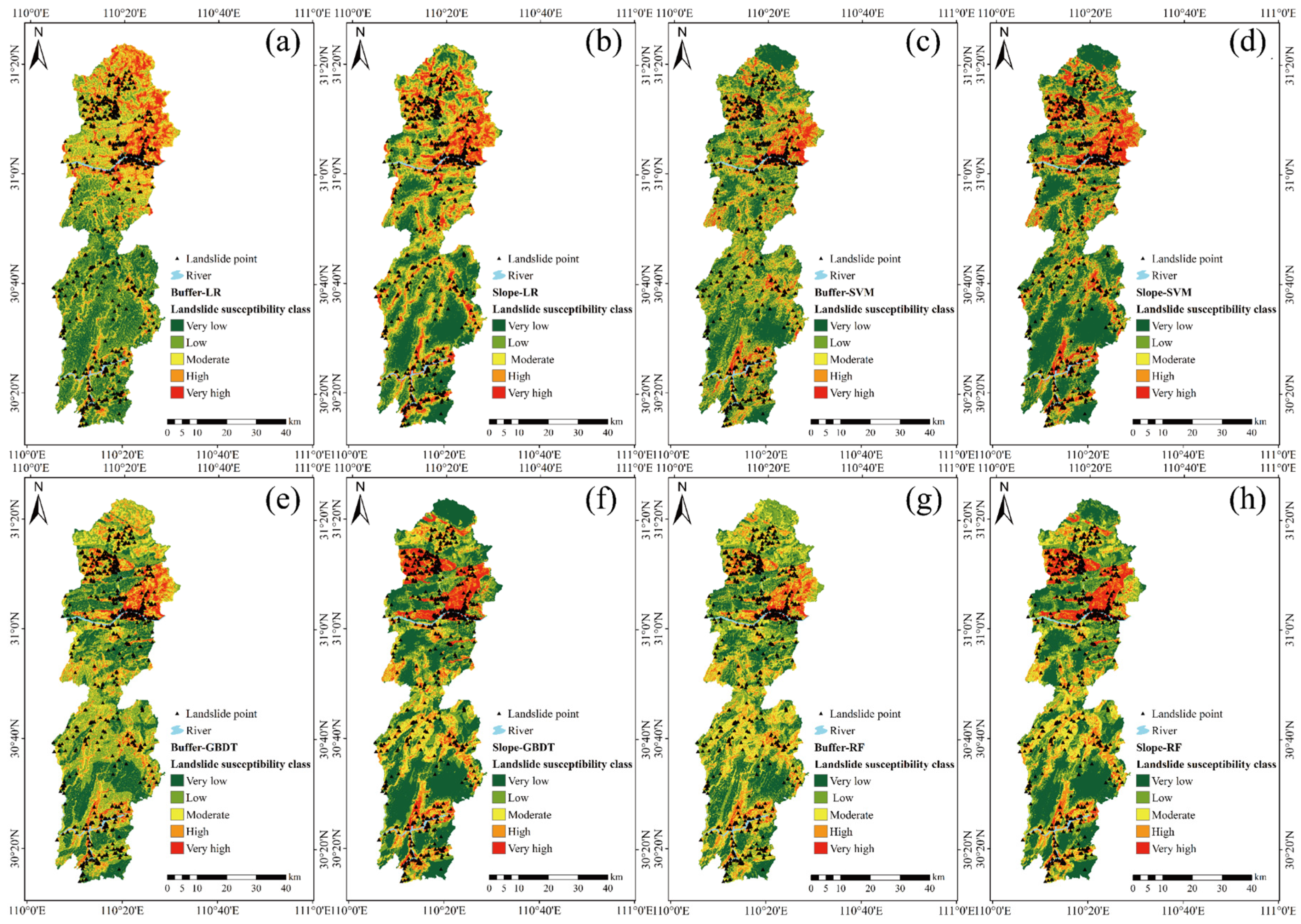
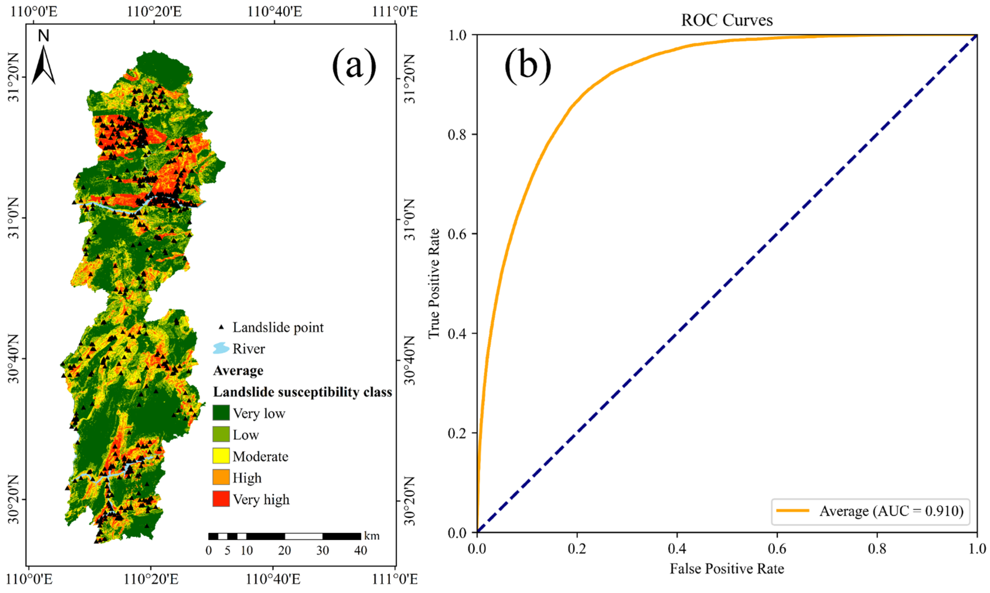
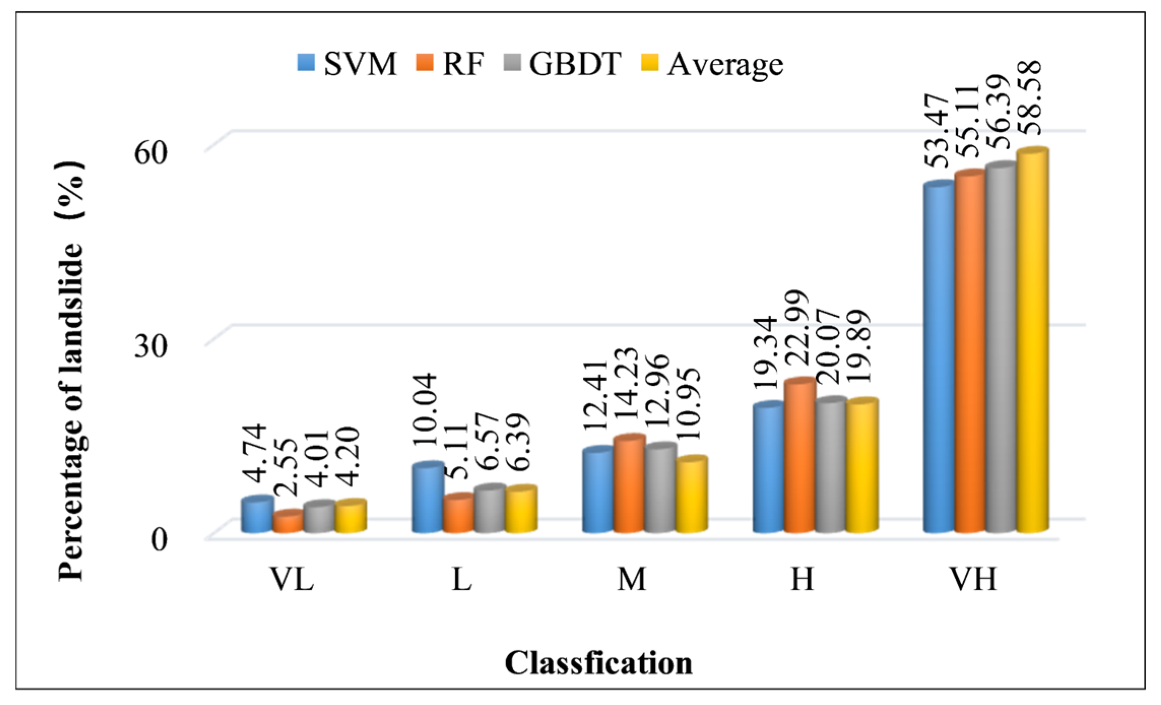
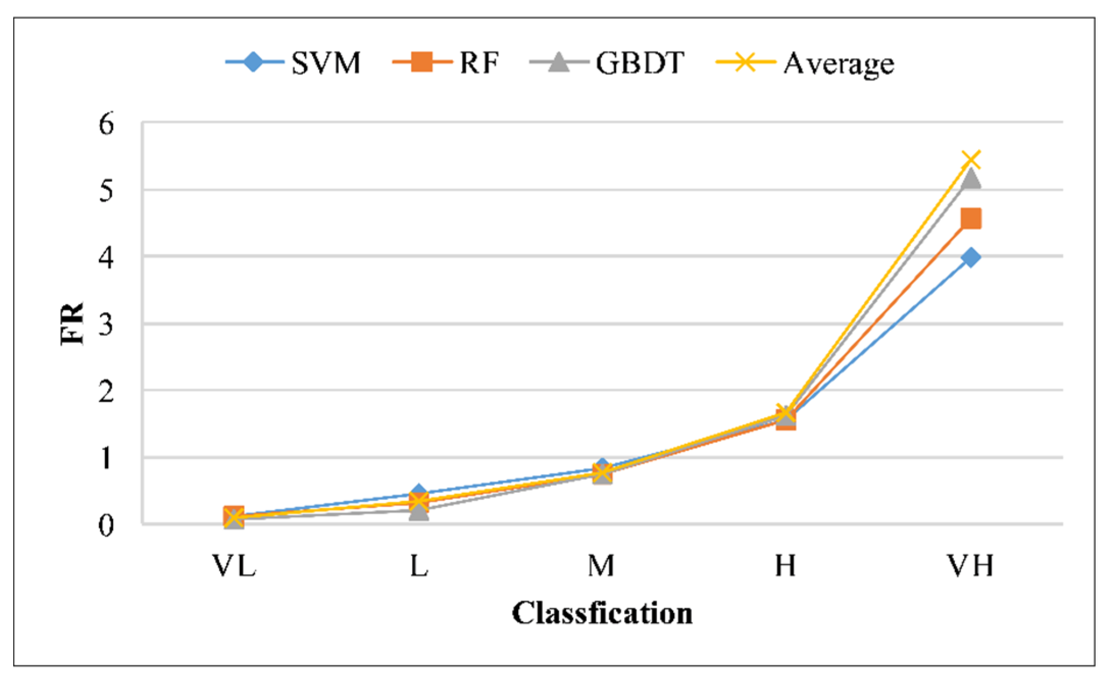
4.1. Landslide Susceptibility Assessment Results

After optimizing the parameters of each model, landslide susceptibility zoning in the study area was conducted using four distinct models. The susceptibility indices produced by these models were imported into ArcGIS, where the natural break method was applied to divide the area into five zones: very low susceptibility (VL), low susceptibility (L), moderate susceptibility (M), high susceptibility (H), and very high susceptibility (VH) (Figure 6). In the figure, Buffer-LR/-SVM/-GBDT/-RF represent the susceptibility maps generated from the “Buffer” dataset, while Slope-LR/-SVM/-GBDT/-RF correspond to the maps derived from the “Slope” dataset. Although the susceptibility zones varied slightly among models, the distributions of the VL and VH zones remained consistent. The VH zones were primarily concentrated in the northern part of Badong County, particularly along rivers, whereas the VL zones were predominantly located in the southern region.

The ROC curves for the eight scenarios are shown in Figure 7. The AUC values for the Buffer-LR/-SVM/-GBDT/-RF models were 0.721, 0.844, 0.829, and 0.824, respectively, whereas the AUC values for the Slope-LR/-SVM/-GBDT/-RF models were 0.763, 0.855, 0.880, and 0.889, respectively. These findings indicated that, irrespective of the machine learning model employed, landslide susceptibility predictions based on non-landslide sample datasets from slope units achieved higher prediction accuracy than those derived from buffer zone datasets.

To evaluate the performance of the four models on unknown data and examine the impact of different sampling strategies on susceptibility results, the accuracy, precision, recall, and F1 score were calculated for each model using the test set.

Table 4. Performance metrics for four models with two sampling strategies.

Model	Accuracy		Precision		Recall		F1 Score
	Buffer	Slope	Buffer	Slope	Buffer	Slope	Buffer	Slope
LR	0.6054	0.7187	0.6037	0.7138	0.6034	0.7282	0.6036	0.7209
SVM	0.7139	0.8040	0.7227	0.7939	0.6967	0.8227	0.7095	0.8080
GBDT	0.7222	0.8312	0.7241	0.8285	0.7202	0.8382	0.7221	0.8321
RF	0.7299	0.8385	0.7381	0.8406	0.7098	0.8341	0.7237	0.8373

presents a detailed comparison of these metrics for the four models under two distinct non-landslide sample selection strategies.

The table revealed that the slope dataset outperformed the buffer dataset across all metrics. Among the models, the RF model demonstrated superior accuracy, precision, and F1 score on both datasets compared with the others.

4.2. Uncertainty in Machine Learning Model Selection

To reduce the impact of model selection uncertainty on landslide susceptibility predictions, the average landslide susceptibility index for each raster cell was computed using susceptibility maps generated with the “Slope” dataset and the SVM, GBDT, and RF models, collectively referred to as the “Average” model. The resulting landslide susceptibility map for Badong County is shown in Figure 8a, and the corresponding ROC curve is presented in Figure 8b. Compared with the individual models, the average method achieved an AUC value of 0.910, reflecting a significant improvement. This demonstrated the effectiveness of the average method in providing a comprehensive analysis of landslide susceptibility results across different models.

The prediction results were evaluated by analyzing the distribution and proportion of existing landslide disaster points across different susceptibility zones. To this end, the proportion of landslides within each susceptibility zone was calculated. The study area was divided into five susceptibility zones (VL, L, M, H, and VH) by using the natural break method. Statistical analysis was performed on the distribution of landslide disaster points, distribution of raster cells within each susceptibility zone generated by each model, and corresponding FR indicators (

Table 5. Statistical analysis of landslide disaster points, raster cells, and FR indicators in different susceptibility zones across various models.

Model	Susceptibility Zones	Raster Cells	Proportion (%)	Landslide Count	Proportion (%)	FR
Slope-SVM	VL	1,371,117	36.84	26	4.74	0.13
	L	827,852	22.25	55	10.04	0.45
	M	559,434	15.03	68	12.41	0.83
	H	462,794	12.44	106	19.34	1.56
	VH	500,315	13.44	293	53.47	3.98
Slope-RF	VL	1,168,148	31.39	14	2.55	0.11
	L	919,426	24.71	28	5.11	0.32
	M	710,896	19.10	78	14.23	0.75
	H	526,665	14.15	126	22.99	1.56
	VH	396,377	10.65	302	55.11	4.56
Slope-GBDT	VL	1,381,568	37.12	22	4.01	0.08
	L	757,638	20.36	36	6.57	0.21
	M	644,561	17.32	71	12.96	0.75
	H	477,588	12.83	110	20.07	1.62
	VH	460,157	12.36	309	56.39	5.17
Average	VL	1,665,281	44.75	23	4.20	0.09
	L	688,898	18.51	35	6.39	0.35
	M	524,041	14.08	60	10.95	0.78
	H	420,368	11.30	109	19.89	1.67
	VH	422,924	11.36	321	58.58	5.44

).

Across all models, the distribution of landslide disaster points increased with higher susceptibility levels within the study area. In all four scenarios, the proportion of landslide disasters in very-low-susceptibility areas remained below 5% (Figure 9), with the RF model showing the lowest proportion at 2.55%. Conversely, the proportion of landslide disasters in the H and VH susceptibility areas exceeded 70% in all scenarios. Notably, in the average scenario, the proportion of landslide disasters in the very high susceptibility zone reached 58.58%, the highest among all scenarios. Distribution of landslide disasters relative to susceptibility zones aligned with objective patterns and logic. The results processed using the average method demonstrated better consistency with logical reasoning and objective reality.

The FR indicator was calculated to represent the relative density of landslides within specific susceptibility zones, considering both the number of landslides and total area of each zone. An effective LSM is typically characterized by higher FR values in the H and VH susceptibility zones. In all four scenarios, the FR values progressively increased with increasing susceptibility levels (Figure 10). The FR values were less than 1 in the VL, L, and M susceptibility zones but exceeded 1 in the H and VH zones, demonstrating that susceptibility zoning accurately captured the spatial distribution of historical landslides. Notably, in the “Average” model, the FR values for the H and VH zones were higher than those in the other scenarios, reaching 1.67 and 5.44, respectively.

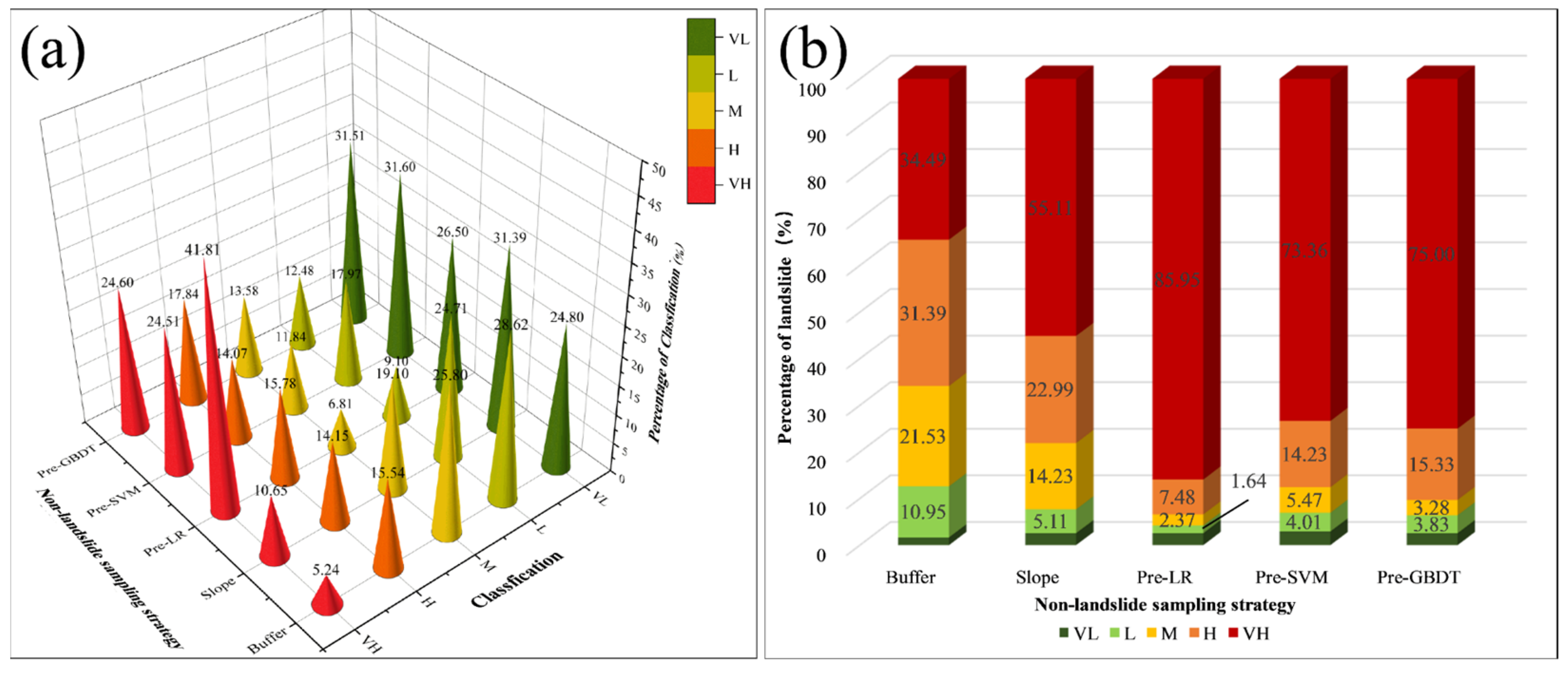
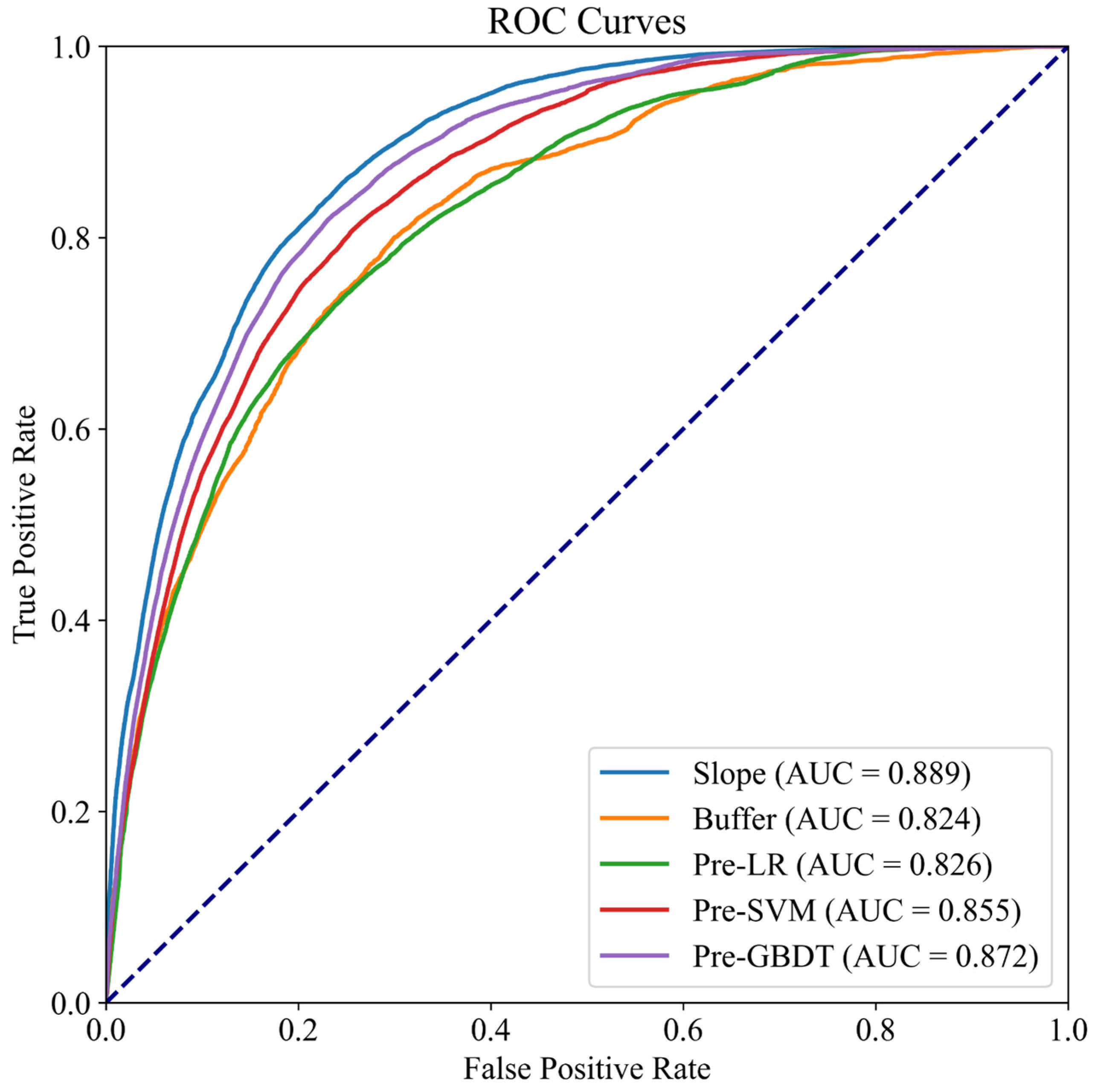
4.3. Impact of Non-Landslide Sample Sampling Strategies on Landslide Susceptibility Assessment

To minimize the uncertainty in selecting non-landslide samples, this study confirmed the advantages of selecting non-landslide samples from slope units without landslides. Subsequently, non-landslide samples were selected from low-susceptibility zones identified by the LR, SVM, and GBDT models on the “Slope” dataset. Landslide susceptibility mapping was conducted for the study area using the RF model, which exhibited a superior predictive performance. The results of the landslide susceptibility zoning under the five non-landslide sampling strategies are shown in Figure 11.

To analyze the distribution patterns of susceptibility zonation and landslides in these LSMs, the area of each susceptibility level was quantified. The results indicated that most VH susceptibility zones typically accounted for 5.24% to 24.60% of the total area. Generally, the L and VL susceptibility zones occupied a larger proportion of the area than the other zones (Figure 12a), except in the “Pre-LR” dataset, where the VH zone covered a significantly larger area, comprising 41.81% of the total. Subsequently, landslide percentages at each susceptibility level were compared. In the “Pre-LR” dataset, the VL zone contained less than 3% of all landslides, whereas the VH zone accounted for 85.95%. In contrast, in the “Buffer” dataset, less than 2% of the landslides fell within the VL zone, whereas 34.49% were located in the VH zone (Figure 12b). These findings suggest that the use of the VL zone from the LR model as a non-landslide dataset yields unsatisfactory results.

ROC curves were plotted for the five scenarios (Figure 13), with the “Slope” dataset achieving the highest AUC value of 0.889. The AUC values for the remaining datasets in descending order were as follows: “Pre-GBDT” at 0.872, “Pre-SVM” at 0.855, “Pre-LR” at 0.826, and “Buffer” at 0.824. These results indicated that the performance of the “Pre-LR” dataset was suboptimal. However, the AUC values exhibited an upward trend with the increasing accuracy of the pre-classification models.

5. Discussion

This section focuses on three key aspects: (1) the primary findings derived from the experimental results; (2) the remaining uncertainties present in the modeling process; and (3) the limitations of this study and suggestions for future research priorities.

The uncertainties that this study seeks to address can be categorized into two main aspects: (1) the effect of non-landslide sample selection on susceptibility modeling; and (2) the impact of machine learning model selection on prediction outcomes. Specifically, when an 800 m buffer was applied around landslide points, the susceptibility zoning generated using non-landslide samples from outside the buffer indicated a significantly lower predictive accuracy than the samples drawn from slope units without landslides. Geologically, this discrepancy can be identified because non-landslide samples from outside the buffer zone may include environments and geological conditions similar to those that favor landslide development [18]. In contrast, selecting non-landslide samples from slope units without landslides effectively eliminated this issue. Statistical analyses, confusion matrix metrics, and AUC values confirmed this finding, demonstrating substantial improvements when the non-landslide samples were selected from slope units devoid of landslides. This study further confirmed that selecting non-landslide samples from the very-low-susceptibility zone identified by machine learning models could enhance susceptibility modeling performance, yielding higher AUC values than selecting non-landslide samples outside the buffer zone. However, the predictive performance was closely tied to the accuracy of the pre-classified machine learning model. Generally, a higher accuracy in the pre-classified model could contribute to better classification performance using the RF model. Conversely, lower accuracy in pre-classified models, such as the LR model in this study, may lead to significant discrepancies between the RF model predictions and actual performance. Additionally, integrating multiple machine learning models has been proven to mitigate the impact of model selection on landslide susceptibility modeling; however, this approach requires inherently high prediction accuracy for each model.

In this study, uncertainties persisted, primarily in two aspects: (1) the selection of landslide samples; and (2) the selection of influencing factors. First, the sampling method for the landslide samples in this study was based on the length and width of the landslides recorded in the landslide catalog data to calculate their area. Then, each landslide was approximately regarded as a circle, with the radius derived from the area. A buffer was created based on the radius, and a portion of the slope unit containing the landslide was extracted as a landslide sample. This method inevitably deviates from the true extent of the landslide area, potentially including non-landslide areas or excluding parts of the actual landslide in the sample. Second, the uncertainty introduced by the selection of influencing factors is closely related to the model’s predictive performance. Although numerous influencing factors have been incorporated into landslide susceptibility modeling, no universally optimal combination of factors exists [39]. Some studies have demonstrated that modifying the selection of factors, by either adding or removing certain factors, can enhance predictive ability [40,41]. In this study, 14 influencing factors were selected based on previous research experience; however, the uncertainty in factor selection was not investigated because it was not the primary focus of our research. Despite these two sources of uncertainty, our results demonstrate that the overall uncertainty in the modeling process is within an acceptable range. The AUC accuracy of all sampling strategies exceeded 0.721, and the ROC values for most strategies exceeded 0.8. This enables us to focus on analyzing the impact of sampling strategies and integrating the results of the different models, rather than solely focusing on improving model performance.

Given the uncertainties mentioned above, the main limitations of the current method and findings can be summarized as follows. First, landslide samples generated by buffering outward from the landslide point may fail to accurately represent the actual landslide area. Using deciphered landslide surface vectors as samples would address this issue. However, this approach can be labor-intensive and challenging to implement. Second, this study focused only on the impact of non-landslide sample selection strategies on susceptibility modeling, while landslide sample selection also played a critical role in influencing the outcomes. For instance, Guo et al. [20] explored three landslide sample selection strategies along the landslide boundary, within the boundary, and in the landslide extension area, highlighting their significant impact on modeling. Similarly, Huang et al. [42] selected two widely used models, SVM and RF, to develop a landslide susceptibility assessment using landslide points, buffer zones, and polygonal surfaces. Furthermore, the models implemented in this study represented only a small subset of the available machine learning methods, limiting the ability to reduce the uncertainty associated with model selection. With limited research in this area, averaging the results from multiple models could offer little basis for meaningful comparisons with other approaches to address model selection uncertainty. Many researchers have explored suitable models for specific study areas by employing various sampling strategies, examining the effects of spatial resolution on susceptibility assessments, and analyzing the influence of different proportions of landslide and non-landslide samples. For example, Hong et al. [43] investigated how different non-landslide sample selection methods and varying ratios of landslide to non-landslide samples affect landslide susceptibility modeling. Chen et al. [44] compared the impact of different spatial resolutions (30, 40, 50, 60, 70, 80, and 90 m) on landslide susceptibility modeling using three models: frequency ratios, entropy indices, and weights of evidence. Yan et al. [45] analyzed the effects of environmental factors at resolutions ranging from 30 to 600 m, with 30 m intervals, on landslide susceptibility assessments. Similarly, Yang et al. [46] investigated the impact of varying ratios of landslide to non-landslide samples on landslide susceptibility modeling using a Bayesian optimization method. Hence, developing and testing alternative sampling techniques for both landslide and non-landslide cases as well as exploring innovative strategies for minimizing model selection uncertainty are essential. These advancements can provide valuable insights and significantly improve LSA.

In conclusion, the improvement observed from selecting non-landslide samples from slope units without landslides and very-low-susceptibility zones identified by pre-classified machine learning models holds significant potential for enhancing the accuracy and reliability of landslide susceptibility modeling. This refinement is particularly valuable for risk assessment and disaster management because it provides a more precise representation of low-susceptibility areas, potentially reducing the occurrence of false positives in landslide predictions. Such refinements could ultimately support more informed decision-making in risk mitigation efforts. This approach may prove instrumental in developing more reliable susceptibility maps and promoting proactive disaster prevention strategies, especially in landslide-prone regions. Additionally, the use of model averaging to mitigate the impact of model selection can be applied to other natural hazard risk assessments, offering benefits to a broader international audience involved in environmental management and disaster preparedness. These findings provide evidence-based strategies for improving susceptibility mapping and risk prediction.

6. Conclusions

The regional LSA and its associated uncertainties remain significant challenges for managing and mitigating landslide risks. This study focused on Badong County and examined the impact of model selection uncertainty and non-landslide dataset sampling strategies on the susceptibility zoning performance. The findings revealed that selecting non-landslide samples from the slope units without landslides substantially improved the accuracy of LSM compared to selecting those outside a designated buffer zone. The confusion matrix metrics and AUC values consistently demonstrated superior performance across the four machine learning models when the slope unit sampling strategy was applied, with the RF model achieving the highest accuracy. The AUC values for the four models showed improvements ranging from 0.011 to 0.065 between the two sampling strategies. Furthermore, using very-low-susceptibility zones identified by nonlinear machine learning models as non-landslide samples enhanced the susceptibility modeling performance, with the effectiveness depending on the accuracy of the pre-classified models. The higher-performing pre-classified models yielded better-performing non-landslide samples. These results suggested that the common strategy of randomly selecting non-landslide samples outside the buffer zone introduced significant uncertainty. Integrating the outputs of various machine learning models using an average method can effectively enhance predictive performance. Metrics such as the AUC and FR confirmed that the averaging method provided a comprehensive analysis of susceptibility outputs from different models, thereby reducing the uncertainty associated with model selection.

This study confirmed that the uncertainties in LSA stemmed in part from the dataset sampling strategies and selection of machine learning models. However, these uncertainties were mitigated by enhancing the quality of non-landslide samples and integrating the average susceptibility indices from multiple models. Accordingly, susceptibility modeling frameworks should adopt robust and well-justified sampling strategies to ensure more reliable results. In addition, utilizing multiple assessment models further minimized the uncertainty associated with the model selection. Future research should focus on examining the effects of different sampling strategies for landslide and non-landslide samples and exploring the influence of varying data resolutions on susceptibility modeling results.

References

1. Segoni, S.; Pappafico, G.; Luti, T.; Catani, F. Landslide susceptibility assessment in complex geological settings: Sensitivity to geological information and insights on its parameterization. Landslides 2020, 17, 2443–2453. [Google Scholar] [CrossRef]
2. Reichenbach, P.; Rossi, M.; Malamud, B.D.; Mihir, M.; Guzzetti, F. A review of statistically-based landslide susceptibility models. Earth-Sci. Rev. 2018, 180, 60–91. [Google Scholar] [CrossRef]
3. Brabb, E.E. Innovative approaches to landslide hazard mapping. In Proceedings of the 4th International Symposium on Landslides, Toronto, ON, Canada, 16–21 September 1984; Canadian Geotechnical Society: Vancouver, BC, Canada, 1984; Volume 1, pp. 307–324. [Google Scholar]
4. Guzzetti, F.; Carrara, A.; Cardinali, M.; Reichenbach, P. Landslide hazard evaluation: A review of current techniques and their application in a multi-scale study. Geomorphology 1999, 31, 181–216. [Google Scholar] [CrossRef]
5. Akgun, A.; Kincal, C.; Pradhan, B. Application of remote sensing data and GIS for landslide risk assessment as an environmental threat to Izmir city (West Turkey). Environ. Monit. Assess. 2011, 184, 5453–5470. [Google Scholar] [CrossRef]
6. Zhang, W.; Tang, L.; Li, H.; Wang, L.; Cheng, L.; Zhou, T.; Chen, X. Probabilistic stability analysis of Bazimen landslide with monitored rainfall data and water level fluctuations in Three Gorges Reservoir, China. Front. Struct. Civ. Eng. 2020, 14, 1247–1261. [Google Scholar] [CrossRef]
7. Abedini, M.; Tulabi, S. Assessing LNRF, FR, and AHP models in landslide susceptibility mapping index: A comparative study of Nojian watershed in Lorestan province, Iran. Environ. Earth Sci. 2018, 77, 405. [Google Scholar] [CrossRef]
8. Pham, B.T.; Pradhan, B.; Bui, D.T.; Prakash, I.; Dholakia, M.B. A comparative study of different machine learning methods for landslide susceptibility assessment: A case study of Uttarakhand area (India). Environ. Model. Softw. 2016, 84, 240–250. [Google Scholar] [CrossRef]
9. Guo, Z.; Tian, B.; Li, G.; Huang, D.; Zeng, T.; He, J.; Song, D. Landslide susceptibility mapping in the Loess Plateau of northwest China using three data-driven techniques: A case study from middle Yellow River catchment. Front. Earth Sci. 2023, 10, 1033085. [Google Scholar] [CrossRef]
10. Liu, Z.; Zhang, Q.; Wang, Y.; Li, X.; Zhang, Y. Application of logistic regression for landslide susceptibility mapping in mountainous areas: A case study of the Wuling Mountains, China. Landslides 2022, 19, 87–102. [Google Scholar]
11. Jafari, A.; Chai, W.; Zhang, H.; Li, M. Landslide susceptibility assessment using k-nearest neighbor algorithm in the southwestern region of China. Geomorphology 2021, 387, 107785. [Google Scholar]
12. Li, P.; Yang, C.; Zhang, L.; Liu, Z. A novel landslide susceptibility mapping approach using support vector machine with the integration of geological and topographical factors. Environ. Earth Sci. 2023, 82, 345. [Google Scholar]
13. Zhang, W.; Li, J.; Wang, L.; Liu, Y. Landslide susceptibility mapping using extremely randomized trees: A case study in the Qinling Mountains, China. Nat. Hazards 2022, 112, 45–61. [Google Scholar]
14. Zhou, X.; Wang, L.; Zhao, Q.; Li, J. Landslide susceptibility modeling using Bayesian networks: A case study of the Sichuan Basin, China. Sci. Total Environ. 2021, 783, 146993. [Google Scholar]
15. Xu, Z.; Zhao, Q.; Liu, H.; Zhang, W. Landslide susceptibility assessment using artificial neural networks in the Loess Plateau, China. Geomorphology 2022, 400, 107836. [Google Scholar]
16. Wang, M.; Liu, Y.; Chen, X.; Zhang, J. Gradient boosting decision tree for landslide susceptibility modeling: A case study of the Three Gorges Reservoir Area, China. Landslides 2023, 20, 289–302. [Google Scholar]
17. Zhang, X.; Chen, J.; Liu, Y.; Li, S. Landslide susceptibility mapping using random forest: Application to the Tibetan Plateau. Environ. Monit. Assess. 2023, 195, 468. [Google Scholar]
18. Chang, Z.L. Regional Rainfall-Induced Landslide Hazard Assessment Method Based on Data-Driven and Forming Mechanism. Ph.D. Thesis, Nanchang University, Nanchang, China, 2023. (In Chinese). [Google Scholar]
19. Xi, C.J.; Han, M.; Hu, X.W.; Liu, B.; He, K.; Luo, G.; Cao, X.C. Effectiveness of Newmark-based sampling strategy for coseismic landslide susceptibility mapping using deep learning, support vector machine, and logistic regression. Bull. Eng. Geol. Environ. 2022, 81, 174. [Google Scholar] [CrossRef]
20. Guo, Z.; Tian, B.; Zhu, Y.; He, J.; Zhang, T. How do the landslide and non-landslide sampling strategies impact landslide susceptibility assessment? A catchment-scale case study from China. J. Rock Mech. Geotech. Eng. 2024, 16, 877–894. [Google Scholar] [CrossRef]
21. Choi, J.; Oh, H.J.; Won, J.S.; Lee, S. Validation of an artificial neural network model for landslide susceptibility mapping. Environ. Earth Sci. 2010, 60, 473–483. [Google Scholar] [CrossRef]
22. Azarafza, M.; Azarafza, M.; Akgün, H.; Atkinson, P.M.; Derakhshani, R. Deep learning-based landslide susceptibility mapping. Sci. Rep. 2021, 11, 24112. [Google Scholar] [CrossRef] [PubMed]
23. Wang, Q.; Wang, Y.; Niu, R.; Peng, L. Integration of information theory, K-means cluster analysis and the logistic regression model for landslide susceptibility mapping in the Three Gorges Area, China. Remote Sens. 2017, 9, 938. [Google Scholar] [CrossRef]
24. Lucchese, L.V.; de Oliveira, G.G.; Pedrollo, O.C. Investigation of the influence of nonoccurrence sampling on landslide susceptibility assessment using artificial neural networks. Catena 2021, 198, 105067. [Google Scholar] [CrossRef]
25. Liu, H.; Zhang, L.; Wang, X. Application of Digital Elevation Model (DEM) in Landslide Susceptibility Mapping: A Case Study. Landslides 2020, 15, 123–135. [Google Scholar]
26. Wang, J.; Li, Z.; Yang, M. Role of Geological Data in Landslide Risk Assessment. Geol. Sci. 2019, 12, 223–234. [Google Scholar]
27. Wang, Y.; Li, Q.; Zhang, Y.; Chen, L. Landslide susceptibility assessment using spatial interpolation of rainfall data: A case study of the Xijiang River Basin. Landslides 2021, 18, 665–678. [Google Scholar]
28. Yang, S.; Zhao, X.; Wang, B. Relationship Between Vegetation Cover (NDVI) and Landslide Susceptibility. Environ. Earth Sci. 2020, 8, 340–350. [Google Scholar]
29. Zhao, W.; Liu, Z.; Li, G. Impact of Land Use and Vegetation on Landslide Hazard Assessment. Nat. Hazards J. 2018, 30, 215–228. [Google Scholar]
30. Shirzadi, A.; Chapi, K.; Shahabi, H.; Solaimani, K.; Kavian, A.; Ahmad, B.B. Rockfall susceptibility assessment along a mountainous road: An evaluation of bivariate statistic, analytical hierarchy process, and frequency ratio. Environ. Earth Sci. 2017, 76, 152. [Google Scholar] [CrossRef]
31. Pearson, K. Note on Regression and Inheritance in the Case of Two Parents. Proc. R. Soc. Lond. 1895, 58, 240–242. [Google Scholar]
32. Nelder, J.A.; Baker, R.J. Generalized Linear Models; Wiley Online Library: Hoboken, NJ, USA, 2006. [Google Scholar]
33. Friedman, J.H. Greedy function approximation: A gradient boosting machine. Ann. Stat. 2001, 29, 1189–1232. [Google Scholar] [CrossRef]
34. Cortes, C.; Vapnik, V. Support-vector networks. Mach. Learn. 1995, 20, 273–297. [Google Scholar] [CrossRef]
35. Cristianini, N.; Schoelkopf, B. Support vector machines and kernel methods: The new generation of learning machines. AI Mag. 2002, 23, 31–41. [Google Scholar]
36. Breiman, L. Random forests. Mach. Learn. 2001, 45, 5–32. [Google Scholar] [CrossRef]
37. Fang, K.; Wu, J.; Zhu, J. A review of technologies on random forests. Stat. Inform. Forum. 2011, 26, 32–38. [Google Scholar]
38. Rodrigues, S.G.; Silva, M.M.; Alencar, M.H. A proposal for an approach to mapping susceptibility to landslides using natural language processing and machine learning. Landslides 2021, 18, 2515–2529. [Google Scholar] [CrossRef]
39. van Westen, C.J.; van Asch, T.W.J.; Soeters, R. Landslide hazard and risk zonation: Why is it still so difficult? Bull. Eng. Geol. Environ. 2006, 65, 167–184. [Google Scholar] [CrossRef]
40. Pham, B.T.; Jaafari, A.; Prakash, I.; Bui, D.T. A novel hybrid intelligent model of support vector machines and the MultiBoost ensemble for landslide susceptibility modeling. Bull. Eng. Geol. Environ. 2019, 78, 2865–2886. [Google Scholar] [CrossRef]
41. Tang, Y.; Feng, F.; Guo, Z.; Feng, W.; Li, Z.; Wang, J.; Sun, Q.; Ma, H.; Li, Y. Integrating principal component analysis with statistically-based models for analysis of causal factors and landslide susceptibility mapping: A comparative study from the loess plateau area in Shanxi (China). J. Clean. Prod. 2020, 277, 124159. [Google Scholar] [CrossRef]
42. Huang, F.; Yan, J.; Fan, X.; Zhang, Y.; Liu, Z.; Wang, Q.; Chen, J.; Liu, L. Uncertainty pattern in landslide susceptibility prediction modelling: Effects of different landslide boundaries and spatial shape expressions. Geosci. Front. 2022, 13, 101317. [Google Scholar] [CrossRef]
43. Hong, H.; Miao, Y.; Liu, J.; Zhang, C.; Yang, L.; Zhao, Z. Exploring the effects of the design and quantity of absence data on the performance of random forest-based landslide susceptibility mapping. Catena 2019, 176, 45–64. [Google Scholar] [CrossRef]
44. Chen, Z.; Ye, F.; Fu, W.; Wu, G.; Zhang, T.; Wang, Q. The influence of DEM spatial resolution on landslide susceptibility mapping in the Baxie River basin, NW China. Nat. Hazards 2020, 101, 853–877. [Google Scholar] [CrossRef]
45. Yan, G.; Tang, G.; Li, S.; Zhang, Y.; Wang, X.; Xu, Y. Uncertainty in regional scale assessment of landslide susceptibility using various resolutions. Nat. Hazards 2023, 117, 399–423. [Google Scholar] [CrossRef]
46. Yang, C.; Liu, L.L.; Huang, F.; Chen, Y.; Zhang, H.; Li, J.; Wang, F. Machine learning-based landslide susceptibility assessment with optimized ratio of landslide to non-landslide samples. Gondwana Res. 2022, 123, 198–216. [Google Scholar] [CrossRef]
Figure 1. Distribution of landslide disasters and geographic locations in Badong County.
Applsci 15 02132 g001
Figure 2. Influencing factors used: (a) elevation; (b) slope; (c) aspect; (d) curvature; (e) distance to fault; (f) EGRG; (g) slope structure; (h) distance to river; (i) TWI; (j) flow path length; (k) flow width; (l) mean annual rainfall; (m) land use type; and (n) NDVI.
Applsci 15 02132 g002
Figure 3. Research flowchart. LR, logistic regression model; SVM, support vector machine model; GBDT, gradient boosting decision tree model; RF, random forest model.
Applsci 15 02132 g003
Figure 4. Correlation coefficients between influencing factors.
Applsci 15 02132 g004
Figure 5. Non-landslide sample selection methods: (a) Slope dataset; (b) Buffer dataset.
Applsci 15 02132 g005
Figure 6. Susceptibility zoning maps generated by different machine learning models based on two sampling methods: (a) Buffer-LR; (b) Slope-LR; (c) Buffer-SVM; (d) Slope-SVM; (e) Buffer-GBDT; (f) Slope-GBDT; (g) Buffer-RF; and (h) Slope-RF.
Applsci 15 02132 g006
Figure 7. ROC curves and AUC values for each model based on two datasets: (a) Buffer dataset; (b) Slope dataset.
Applsci 15 02132 g007
Figure 8. (a) LSM obtained using the average method; (b) the corresponding ROC curve and AUC values.
Applsci 15 02132 g008
Figure 9. Statistics of the proportion of landslides in different susceptibility zones of the four models.
Applsci 15 02132 g009
Figure 10. FR of each model at different susceptibility levels.
Applsci 15 02132 g010
Figure 11. LSM for different sampling strategies. LSM is generated by (a) “Pre-LR” datasets (b) “Pre-SVM” datasets (c) “Pre-GBDT” datasets (d) “Buffer” datasets and (e) “Slope” datasets.
Applsci 15 02132 g011
Figure 12. Proportions of areas and landslides across different susceptibility zones under various non-landslide sample sampling strategies: (a) area proportions; (b) landslide proportions.
Applsci 15 02132 g012
Figure 13. ROC curves and AUC values plotted using five different datasets.
Applsci 15 02132 g013