Software Fault Localization Based on SALSA Algorithm

Abstract

In software development, debugging is the most tedious and time-consuming phase. Therefore, various automated fault localization techniques have been proposed to assist debugging. Among existing fault localization techniques, Spectrum-Based Fault Localization (SBFL) is one of the most extensively researched methods. Traditional SBFL techniques rely solely on the coverage of program execution for fault localization, which means they neglect the interactions between program entities and fault propagation paths during the execution of the program, resulting in a tie problem that reduces the accuracy of fault localization. To solve the above problem, this paper proposes SA-SBFL, a fault localization method based on the SALSA (Random Method for Link Structure Analysis) algorithm. First, a link graph of program entities is constructed, which includes interactions between program entities and fault propagation paths. Then, the suspicion values obtained from traditional SBFL methods are used as the initial weights of the link graph. Finally, the random walk model is employed to simulate the propagation of faults among program entities, analyze the importance of program entities in the fault propagation process, and obtain a ranking list of suspicious program entities. The experiments in this paper demonstrate that the SA-SBFL method significantly outperforms general SBFL methods. For instance, in the Defects4J dataset, the SA-SBFL technique outperforms traditional SBFL in terms of fault localization accuracy, with a 47% improvement in the Top-1 metric and a 10% increase in the Top-5 metric, and it also showed an average improvement of 19% in the EXAM metric.

1. Introduction

In today’s rapidly developing software industry, software debugging is a key link in ensuring software quality and reliability [1]. With the increasing complexity and expansion of software systems, the debugging process is becoming increasingly challenging. Software debugging not only helps developers identify and fix errors or defects in the program, but it is also essential for preventing potential system failures, improving user satisfaction, and reducing maintenance costs [2].

Effective software debugging strategies typically include fault localization, which is a core part of the debugging process. In practical software engineering applications, the efficiency and accuracy of fault localization significantly impacts the development cycle and costs. Rapid and accurate fault localization can substantially reduce the time developers spend on debugging, thereby accelerating software release schedules. Additionally, by minimizing system failures caused by errors, software stability and user satisfaction can be enhanced. Traditional fault localization methods often rely on developers’ experience, intuition, and manual code reviews, which are not only time-consuming and labor-intensive but also prone to human error [3]. For instance, in large-scale software projects, even minor errors can lead to system crashes or performance degradation, and traditional fault localization methods may take hours or even days to identify the root cause of the problem. To overcome these limitations, researchers have begun to explore automated and semi-automated fault localization techniques.

Among these emerging technologies, software fault localization techniques based on spectrum have attracted widespread attention due to their unique advantages. Traditional spectrum-based software fault localization techniques determine the code areas that may contain defects by analyzing the coverage of the tested program after execution. Specifically, they utilize the execution information of the tested program (such as covered statements, branches, or paths) and the corresponding test results (success or failure), and assess the risk level of each statement through statistical methods [4]. The core idea of this method is that if a test case fails, the statements it covers are more likely to contain defects. However, Spectrum-Based Fault Localization (SBFL) suffers from the tie problem, where multiple statements within the same basic block may have the same suspicion value, making it impossible to locate the specific faulty statement in the program precisely. This situation severely affects the developers’ debugging efficiency because it leads to a vague indication rather than a clear fault point. To address this issue, researchers have proposed various improvement methods, including methods based on metric combination [5], improving program matrices [6], considering fault propagation context [7], considering local dependency relationships [8], and utilizing program slicing [9,10] to solve this problem. With the development of various technologies and tools, combining traditional software fault localization techniques and different methodologies is a mainstream direction of current research. Some researchers combine the trajectory of program execution with graph theory to study its network structure for precise localization.

Based on the concepts of graph theory, various network analysis algorithms have been invented to analyze the structure of network links and assess the importance of nodes. In recent years, software fault localization techniques based on various network analysis algorithms have achieved certain effects. These methods use abstract syntax trees (AST) [11], Control Flow Graphs (CFG) [12], and Program Dependency Graphs (PDG) [13] as intermediate data representations, abstracting code structure into graph structures. However, when facing large-scale programs, directly constructing a graph from the source code can result in a very large graph, which can severely affect the efficiency of network structure analysis.

In response to this, this paper proposes a software fault localization method based on the SALSA algorithm (SA-SBFL), which aims to address the tie problem that exists in traditional SBFL techniques. Additionally, we consider the control dependency relationships between statements during the execution of the tested program, enabling more precise fault statement localization. Specifically, first, we need to construct the Root Set Control Dependency Graph (RSCDG) based on the execution trajectory of the tested program. This graph is a part of the entire control dependency graph and includes the process of fault propagation. Then, we employ the Stochastic Approach for Link-Structure Analysis (SALSA) algorithm, leveraging the algorithm to analyze the importance of nodes and rank them, thereby achieving accurate localization. The main contributions of this paper are as follows:

(1)

In response to the situation where previous researchers directly abstracted source code into graph structures, which often included a lot of unimportant information, this paper proposes the Root Set Control Dependency Graph (RSCDG). The RSCDG is a part of the control dependency graph, which not only reduces the computational burden on the computer but also contains key information related to the propagation of software faults.

(2)

This paper proposes SA-SBFL, a method based on the principles of the SALSA algorithm, which analyzes the statement link relationships in software fault propagation to achieve accurate fault localization. Additionally, SA-SBFL can effectively address the tie problem present in traditional SBFL techniques.

(3)

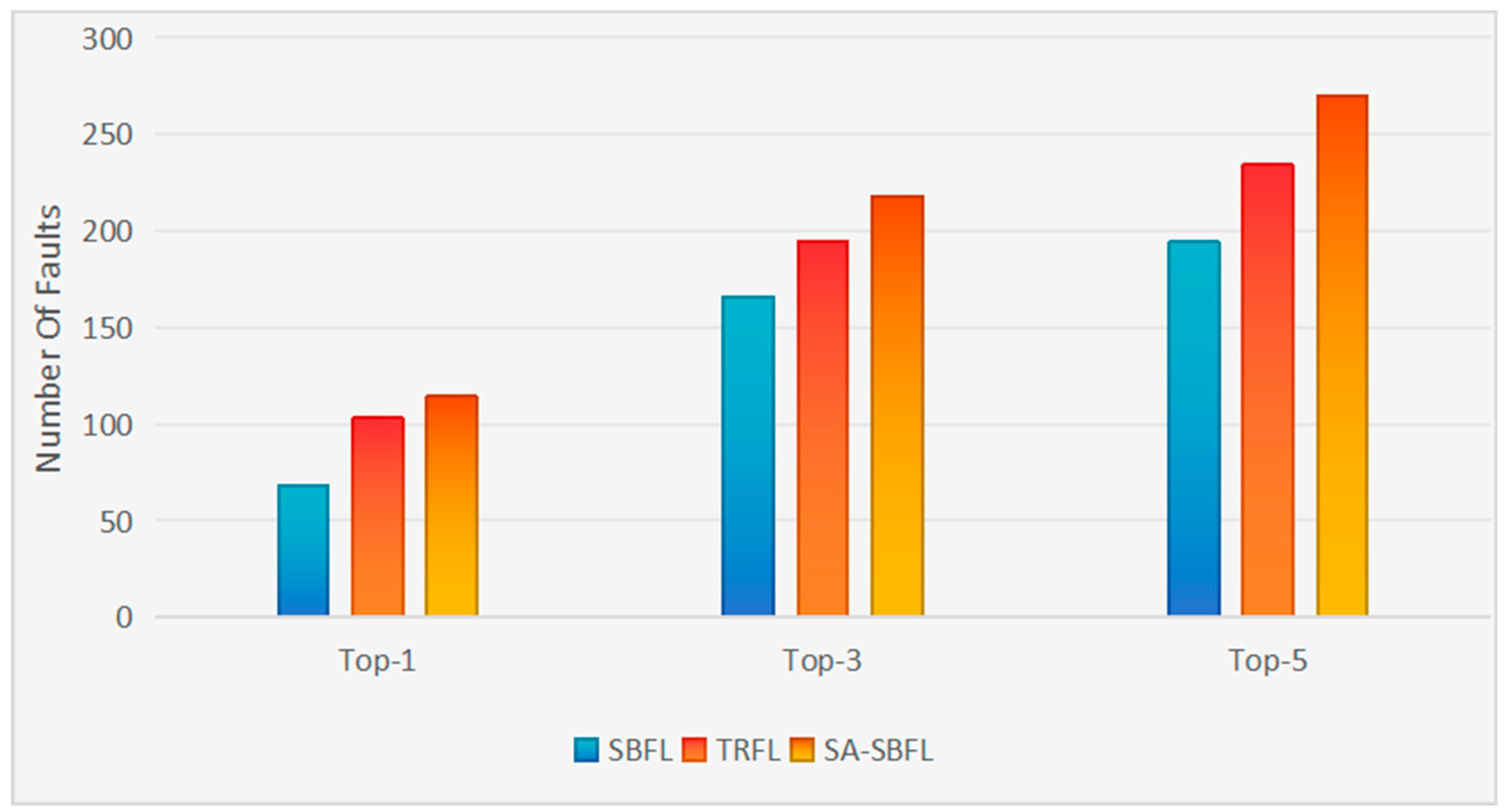
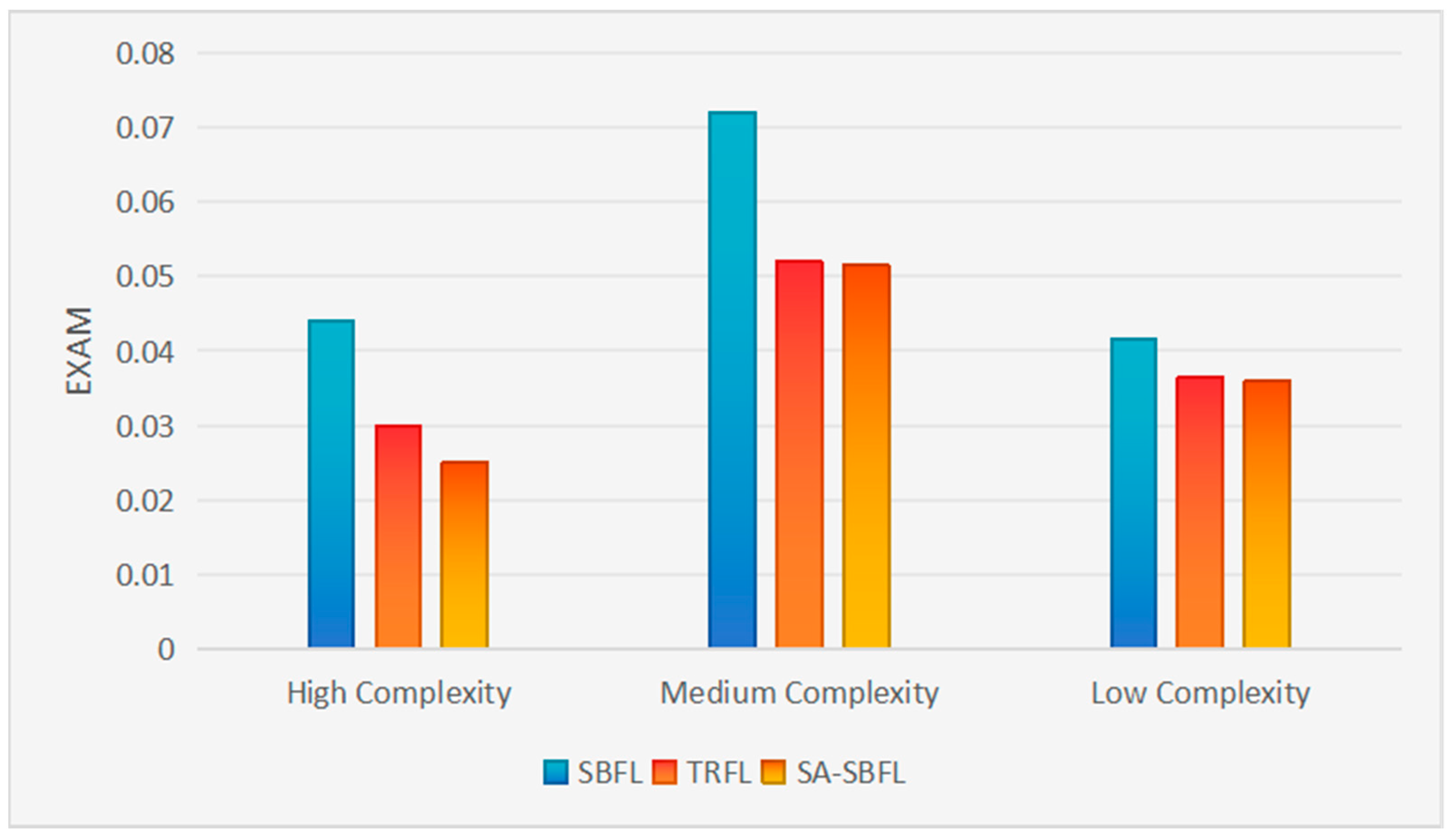
This paper conducted experiments on SA-SBFL using five benchmark projects from Defects4J and evaluated the experimental results with two metrics: Top-N (N = 1, 3, 5) and Expected Additional Mistakes. The experimental results demonstrate that, compared to traditional SBFL techniques, SA-SBFL has better performance.

The remaining research work of this paper is arranged as follows. Section 2 provides a review of related research on fault localization and introduces the technologies used in this paper; Section 3 details the specific framework of SA-SBFL; Section 4 introduces the experimental dataset and evaluation metrics used in this paper; Section 5 discusses the main research questions and the experimental results; Section 6 and Section 7 offer a summary and provide an outlook on future research work.

2. Related Work

2.1. Spectrum-Based Software Fault Localization

Spectrum-Based Fault Localization (SBFL) is a typical method in dynamic analysis. The input for SBFL consists of code coverage information from all test cases, and the output is a list of code elements sorted in descending order of their suspicious values calculated by specific formulas. The “spectrum” in SBFL refers to the collection of code coverage information during the execution of the tested program, which is composed of information about the parts of the program that are executed during the test case execution. This information can include statements, basic blocks, branches, or functions.

To more intuitively reflect the information about the location of defective program entities within the spectrum, Jones et al. proposed a statistical formula known as Tarantula [14]. They speculated that statements covered by failed test cases have a higher degree of suspicion than those covered by successful test cases. Since the introduction of the Tarantula formula, researchers have proposed a variety of suspect value calculation methods. These include the Jaccard formula based on cluster analysis [15], the Ochiai formula inspired by biology [16], the Ochiai 2 formula that considers the impact of unexecuted or passed test cases [17], the Op2 formula, which performs optimally in single fault localization [17], and the Dstar formula [18], which has been proven to have the best comprehensive ranking performance. Nevertheless, no single statistical formula can perfectly adapt to the needs of all test programs [19].

Many current software fault localization methods have been researched and developed based on traditional Spectrum-Based Fault Localization (SBFL) techniques. For instance, Zhao et al. [8] considered the variability among test cases. On the basis of the original spectrum information, they utilized the PageRank algorithm to account for the contribution of different test cases and recalculated the spectrum. Subsequently, they applied traditional SBFL techniques on the recalculated spectrum to achieve more effective fault localization. De Souza et al. [20] improved the effectiveness of SBFL technology in fault localization by introducing context information and filtering strategies. He et al. considered the interactions between software entities and the propagation of influences to construct a Fault Influence Network (FIN) based on the complex network theory, calculating node weights to improve the accuracy of fault localization [21]. Thanks to the efforts of many researchers, Spectrum-Based Software Fault Localization (SBFL) has achieved numerous results. However, as software programs become increasingly complex and larger in scale, relying solely on spectra and statistical formulas is insufficient to pinpoint the location of faults accurately. Building on this, this paper takes into account the interaction between program statements and the propagation paths of faults during the execution process.

2.2. Software Fault Localization Based on Network Analysis Algorithm

Network analysis algorithms assess the importance and relevance of nodes in a network by analyzing the structure of links and relationships between nodes. Therefore, software fault localization methods based on network analysis algorithms can mine critical information from the network structure of source code or program execution paths, thereby completing the fault localization task. X Fan et al. [22] proposed a fault localization technique based on the TrustRank algorithm (TRFL). TRFL combines the internal data dependency relationships of the program to construct a node-weighted program execution network, and uses the TrustRank algorithm to analyze network centrality, thereby re-ranking program entities based on their degree of suspicion. Yan Y et al. [23] proposed a fault localization method based on the PageRank algorithm and mutation analysis (PRMA). This method first applies the PageRank algorithm to calculate the fault scores of statements, then uses these fault scores to weight the suspicion values of statements to address the tie issue in mutation-based fault localization. Finally, statements are ranked based on their weighted suspicion values. Zhang et al. [24] utilized the PageRank algorithm to recalculate the spectral information, taking into account the contributions of different tests, and then applied traditional SBFL techniques on the recalculated spectral information for more effective fault localization. Considering the advantages of network analysis algorithms, we have also employed network analysis algorithms to accomplish the task of fault localization in our research.

2.3. Program Dependency Graph

The Program Dependency Graph (PDG) is a graph structure used to represent the dependencies between various statements in a program. It is an extension of the Control Flow Graph (CFG), encompassing not only the execution path information of the program but also the dependencies of data flow and control flow. It has been widely applied in software testing and program slicing.

Podgurski A et al. [25] summarized the necessity of weak and strong syntactic dependencies for certain inter-statement relationships and pointed out that these dependencies can be efficiently computed to guide activities such as test data selection and code inspection. Harrold M J et al. [26] proposed a fault classification and fault injection method based on the Program Dependence Graph (PDG). This method further characterizes faults by analyzing the differences between the PDGs of the original and faulty programs, categorizing faults into structural and statement-level faults. By performing transformations on the PDG, it generates different types of faults. The Control Dependency Graph (CDG), as a part of the Program Dependency Graph (PDG), specifically represents the control dependency relationships between program statements. This paper takes the CDG as the research object to accomplish the task of fault localization.

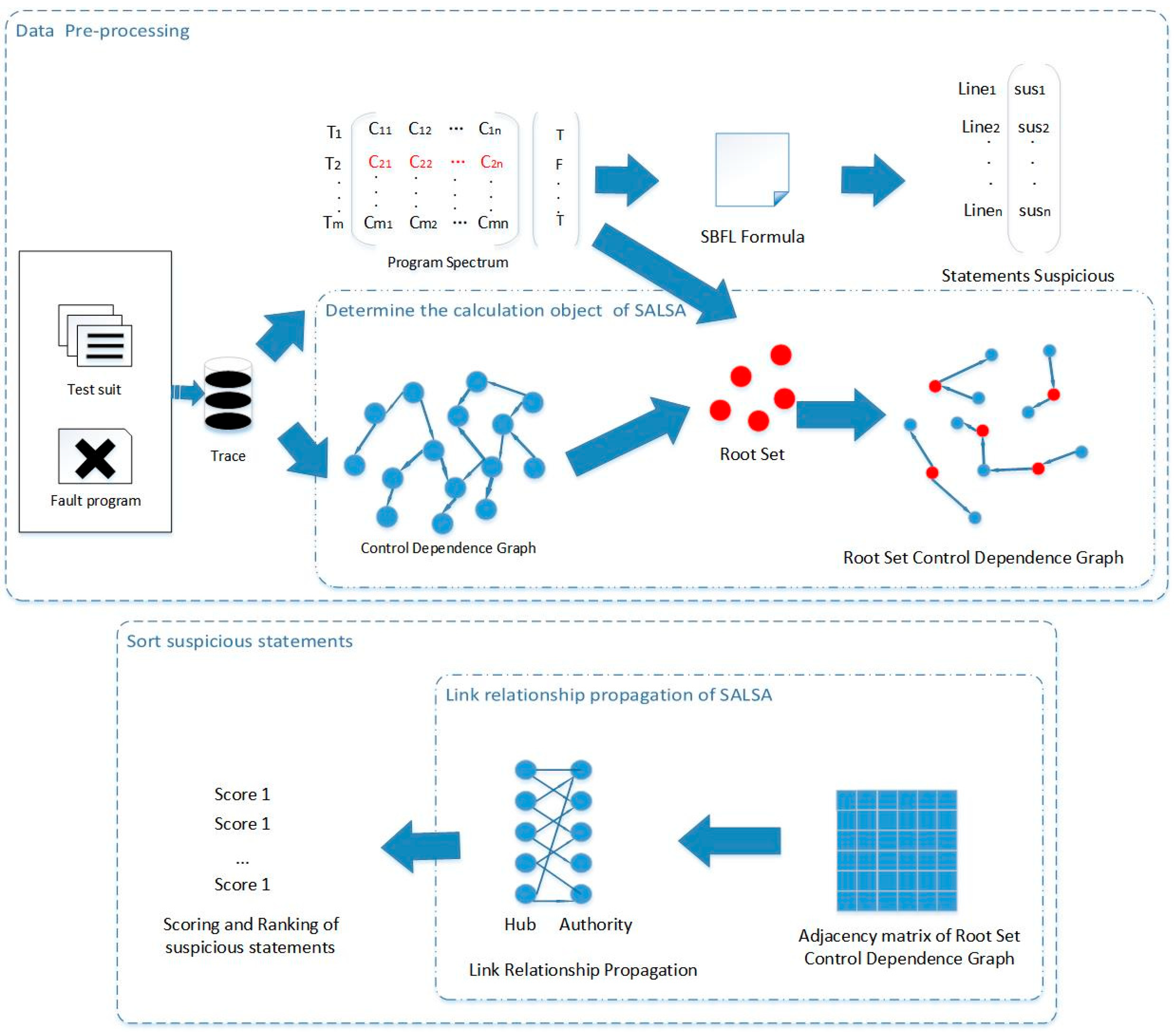
3. Proposed Approach

This paper proposes a software fault localization method based on the SALSA algorithm (SA-SBFL). The full name of the SALSA is Stochastic Approach for Link-Structure Analysis, which is a network analysis algorithm that combines the features of PageRank and HITS algorithms. The specific implementation process of SA-SBFL is derived from the implementation flow of the SALSA algorithm. The computational flow of the SALSA algorithm is divided into two phases: the first is the stage of determining the computation set, and the second is the link relationship propagation phase. Correspondingly, SA-SBFL is also divided into two phases: the first is the data preprocessing phase, the goal of which is to obtain the computation object set; the second phase is the suspicious statement ranking phase, where link relationship propagation is conducted based on the data obtained from the first phase, ultimately leading to the ranking of suspicious statements.

The overall framework is shown in Figure 1, mainly consisting of two stages. (1) Data Preprocessing Stage: First, obtain the project source code from the Defects4j dataset, execute the corresponding test suite, and acquire the program spectrum. Based on the suspicion value calculation formula, determine the suspicion value for each statement. Then, identify the root set (RS) according to the program spectrum, which includes statements strongly related to the fault. Construct the control dependency graph and derive the Root Set Control Dependency Graph (RSCDG) based on the root set. The RSCDG contains the propagation path of the fault and simultaneously narrows down the localization scope. (2) Suspicious Statement Ranking Stage: The suspicion values of statements obtained in the first phase serve as the initial weights of nodes in the RSCDG. The weight of each node is propagated based on the link relationships within the RSCDG, and ultimately, the suspicion values of the statements are output and ranked.

3.1. Data Pre-Processing

3.1.1. Program Spectrum

In the experimental process of this paper, for each faulty version of the program in the Defects4J dataset, the first step is to execute the test suite corresponding to the faulty version to obtain the program’s execution trajectory and generate the spectrum. Program spectrum, also known as code coverage, is a very important concept in the field of software defect localization. It can be defined as the set of program entities that are covered during the execution of tests. Spectrum Based Fault Localization (SBFL) technology utilizes information about program entities executed by test cases to indicate which entities are more likely to be defective. The spectrum, often used to describe the behavior of a program, is a projection of the program’s execution trajectory, revealing the active parts of the program during execution and showing the extent to which test cases cover the code. Each element in the spectrum, such as statements or branches, can be marked as executed or not executed, and this information is crucial for identifying testing blind spots and potential defect areas. In this paper, the spectrum used is a statement spectrum. The matrix form of the spectrum is shown in

Table 1. Spectrum in matrix form.

	e1	e2	e3	e4	e5	e6	e7	Result
T1	1	1	1	0	0	1	0	1
T2	1	1	0	1	0	0	1	1
T3	0	0	1	1	0	0	1	0
T4	1	1	1	1	1	1	1	1
T5	0	0	1	0	1	0	1	0
T6	1	1	0	0	1	1	0	1

.

The rows in the table represent each test case; columns 2 to 8 represent the code lines, with 0 indicating not executed and 1 indicating executed; the last column indicates the result of the test case execution, with 0 indicating failure and 1 indicating success.

3.1.2. Obtain Statement Suspicion Values Based on Statistical Formulas

After obtaining the spectrum of the faulty version of the program, the next step is to calculate the suspicion values of program statements using statistical formulas. SBFL employs statistical formulas to compute the suspicion scores for each code entity, which may include formulas such as Tarantula and Ochiai. When calculating suspicion values, it is necessary to select the appropriate statistical formula based on specific circumstances. Different statistical formulas consider various factors when calculating suspicion values, so the right formula must be chosen based on different scenarios.

Table 2. Common statistical formulas for SBFL.

Name	Formula
Dstar	${\displaystyle \frac{{\mathrm{N}}_{\mathrm{e}\mathrm{f}}^2}{{\mathrm{N}}_{\mathrm{e}\mathrm{p}}+{\mathrm{N}}_{\mathrm{n}\mathrm{f}}}}$
Jaccard	${\displaystyle \frac{{\mathrm{N}}_{\mathrm{e}\mathrm{f}}}{{\mathrm{N}}_{\mathrm{e}\mathrm{f}}+{\mathrm{N}}_{\mathrm{n}\mathrm{f}}+{\mathrm{N}}_{\mathrm{e}\mathrm{p}}}}$
Tarantula	${\displaystyle \frac{\frac{{\mathrm{N}}_{\mathrm{e}\mathrm{f}}}{{\mathrm{N}}_{\mathrm{e}\mathrm{f}}+{\mathrm{N}}_{\mathrm{n}\mathrm{f}}}}{\frac{{\mathrm{N}}_{\mathrm{e}\mathrm{f}}}{{\mathrm{N}}_{\mathrm{e}\mathrm{f}}+{\mathrm{N}}_{\mathrm{n}\mathrm{f}}}+\frac{{\mathrm{N}}_{\mathrm{e}\mathrm{p}}}{{\mathrm{N}}_{\mathrm{e}\mathrm{p}}+{\mathrm{N}}_{\mathrm{n}\mathrm{p}}}}}$
Ochiai	${\displaystyle \frac{{\mathrm{N}}_{\mathrm{e}\mathrm{f}}}{\sqrt{({\mathrm{N}}_{\mathrm{e}\mathrm{f}}+{\mathrm{N}}_{\mathrm{n}\mathrm{f}})·({\mathrm{N}}_{\mathrm{e}\mathrm{f}}+{\mathrm{N}}_{\mathrm{e}\mathrm{p}})}}}$
Ochiai2	${\displaystyle \frac{{\mathrm{N}}_{\mathrm{e}\mathrm{f}}·{\mathrm{N}}_{\mathrm{e}\mathrm{p}}}{\sqrt{({\mathrm{N}}_{\mathrm{e}\mathrm{f}}·{\mathrm{N}}_{\mathrm{e}\mathrm{p}})·({\mathrm{N}}_{\mathrm{n}\mathrm{f}}·{\mathrm{N}}_{\mathrm{n}\mathrm{p}})·({\mathrm{N}}_{\mathrm{e}\mathrm{f}}·{\mathrm{N}}_{\mathrm{n}\mathrm{p}})·({\mathrm{N}}_{\mathrm{n}\mathrm{f}}·{\mathrm{N}}_{\mathrm{e}\mathrm{p}})}}}$
OP2	${\mathrm{N}}_{\mathrm{e}\mathrm{f}}-{\displaystyle \frac{{\mathrm{N}}_{\mathrm{e}\mathrm{p}}}{{\mathrm{N}}_{\mathrm{e}\mathrm{p}}+{\mathrm{N}}_{\mathrm{n}\mathrm{p}}+1}}$

lists some commonly used formulas. The four parameters used in the formulas need to be calculated based on the spectrum matrix, and

Table 3. Four parameters in statistical formulas.

Element	Description
Nef	Number of failed tests to execute the program element
Nep	Number of passed tests for executed program elements
Nnf	Number of failed tests for non-executed program elements
Nnp	Number of passed tests for non-executed program elements

demonstrates the meaning of each parameter.

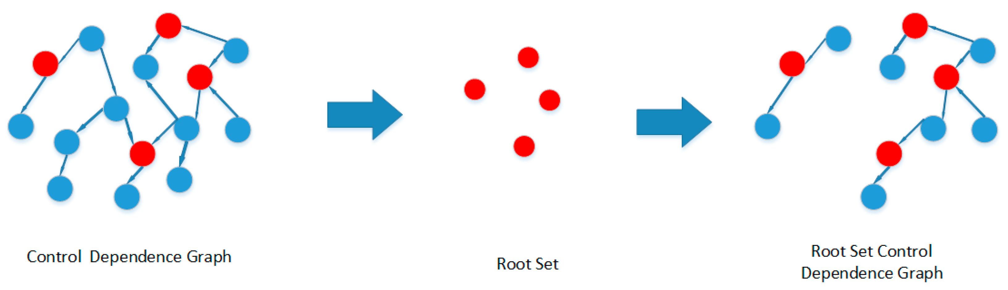
3.1.3. Obtain the Root Set

In the SALSA algorithm, the root set refers to the initial collection of web pages that are highly relevant to the user’s query request. These web pages are considered highly trustworthy and are usually carefully selected based on certain criteria or prior knowledge. The selection of the root set directly affects the trust propagation and node evaluation results across the entire network. Therefore, when choosing the root set, various factors need to be carefully considered to ensure that the selected web pages have sufficient representativeness and credibility. In this paper, the concept of a root set is used, which refers to a collection of statements that are highly related to the fault. Considering that a program statement is more suspicious if it is executed more frequently in failed tests and less frequently in passing tests, this paper analyzes the spectrum to count all program statements in failed test cases and eliminates those that are executed frequently in passing test cases. Ultimately, a set of program statements with high suspiciousness is obtained, known as the root set (RS). Taking the spectrum from Table 1 as an example, RS1 is obtained, which includes e3, e4, e5, and e7.

3.1.4. Obtain the Root Set Control Dependency Graph

The Control Dependency Graph (CDG), as a part of the Program Dependency Graph (PDG), displays the control flow dependency relationships between various statements in a program. In the CDG, nodes represent statements within the program, and edges represent control dependencies, indicating whether the execution of one statement will affect the execution of another statement. This paper introduces the concept of the Root Set Control Dependency Graph (RSCDG), which is a part of the Control Dependency Graph (CDG). The nodes in the RSCDG represent statements that are highly related to the fault, and the edges indicate the propagation of the fault between nodes. The RSCDG corresponds to the expanded web collection in the SALSA algorithm, where the web pages in the expanded web collection are those that have direct linking relationships with the web pages within the root set. Therefore, in this paper, based on the root set obtained from Section 3.1.3, the structures within the CDG that have direct dependency relationships with the statements in the root set are separated to form the RSCDG. Figure 2 illustrates the process of obtaining the RSCDG.

3.2. Sort Suspicious Statements

In this paper, the random walk model is used in this stage to evaluate the importance of nodes in the network structure of the RSCDG. The suspicion values of statements serve as node weights that are propagated along the links between nodes, ultimately resulting in a ranking of suspicious statements.

In the SALSA algorithm, random walk theory and Markov chains are combined to analyze the web page link structure by constructing a bipartite undirected graph, calculating the scores of each node, including Hub scores and Authority scores. This method involves analyzing two distinct Markov chains: the hub chain and the authority chain. In the hub chain, the random walk starts at a hub node, moves to an authority node via an outgoing link, and then returns to another hub node via an incoming link. The hub chain primarily focuses on the out-degree of nodes, that is, how many other nodes a particular node points to. The authority chain is the reverse of the hub chain. The authority chain starts at an authority node, moves to a hub node via an incoming link, and then returns to another authority node via another outgoing link. The authority chain primarily focuses on the in-degree of nodes, that is, how many other nodes point to that particular page. A webpage may score high in the hub chain, indicating that it is an important source of information. At the same time, it may also score high in the authority chain, indicating that it is an important receiver of information.

In this paper, the RSCDG is constructed as an undirected bipartite graph, i.e., RSCDG = (Vh, Va, E). Node set Vh: Contains all nodes with an out-degree greater than 0, which are nodes that point to other nodes. Node set Va: Contains all nodes with an in-degree greater than 0, which are nodes that are pointed to by other nodes. Edge set E: Contains all the linking relationships from one node to another.

In the bipartite graph we derived, we will perform two types of random walks. First, a random walk on the hub chain: starting from a node in Vh, moving to a node on the authority side via an edge, and then returning to a node on the hub side via another edge. Second, a random walk on the authority chain: starting from a node in Va, moving to a node on the hub side via an edge, and then returning to a node on the authority side via another edge. The hub chain simulates a random walk on the hub side, where each state in the chain corresponds to a node in Vh, and transitions between states correspond to walks from one hub node to another through an intermediary authority node. The authority chain simulates a random walk on the authority side, where each state in the chain corresponds to a node in Va, and transitions between states correspond to walks from one authority node to another through an intermediary hub node.

To implement a random walk on a Markov chain, we need to define a transition probability matrix. Since we are conducting random walks on two Markov chains, we need to create two random matrices: the hub matrix H and the authority matrix A. The acquisition of matrices H and A is as follows.

Firstly, based on the linking structure of the RSCDG, we obtain the adjacency matrix W corresponding to the directed graph RSCDG. If node i points to node j, then the value of W_ij is 1; otherwise, it is 0. Then, based on the adjacency matrix W, we obtain the row-normalized matrix W^r and the column-normalized matrix W^c.

The row-normalized matrix W^r is obtained by dividing each non-zero element in W by the sum of the elements in that row. This operation normalizes the sum of each row to 1, representing the probability distribution of links emanating from node i, as shown in Equation (1). Note that if $\sum _{\mathrm{k}=1}^{\mathrm{n}}{\mathrm{W}}_{\mathrm{i}\mathrm{k}}$ = 0, then ${\left({\mathrm{W}}^{\mathrm{r}}\right)}_{\mathrm{i}\mathrm{j}}$ = 0.

$${\left({\mathrm{W}}^{\mathrm{r}}\right)}_{\mathrm{i}\mathrm{j}}={\displaystyle \frac{{\mathrm{W}}_{\mathrm{i}\mathrm{j}}}{\sum _{\mathrm{k}=1}^{\mathrm{n}}{\mathrm{W}}_{\mathrm{i}\mathrm{k}}}}$$

(1)

The column-normalized matrix W^c is derived by dividing each non-zero element in matrix W by the sum of the elements in its corresponding column. This operation normalizes the sum of each column to 1, representing the probability distribution of node j being linked to, as shown in Equation (2). Note that if $\sum _{\mathrm{k}=1}^{\mathrm{n}}{\mathrm{W}}_{\mathrm{k}\mathrm{j}}$ = 0, then ${\left({\mathrm{W}}^{\mathrm{c}}\right)}_{\mathrm{i}\mathrm{j}}$ = 0.

$${\left({\mathrm{W}}^{\mathrm{c}}\right)}_{\mathrm{i}\mathrm{j}}={\displaystyle \frac{{\mathrm{W}}_{\mathrm{i}\mathrm{j}}}{\sum _{\mathrm{k}=1}^{\mathrm{n}}{\mathrm{W}}_{\mathrm{k}\mathrm{j}}}}$$

(2)

Based on the row-normalized matrix W^r and the column-normalized matrix W^c obtained above, we can derive the hub matrix H and the authority matrix A. The hub matrix H is composed of the non-zero rows and columns of W^rW^T_c. This matrix represents the transition probabilities from hub nodes to other hub nodes. The authority matrix is composed of the non-zero rows and columns of W^T_cW^r. This matrix represents the transition probabilities from authority nodes to other authority nodes. Where W^T_c is the transpose of W^c. As shown in Equations (3) and (4).

$$\mathrm{H}={\mathrm{W}}^{\mathrm{r}}{{\mathrm{W}}^{\mathrm{T}}}_{\mathrm{c}}$$

(3)

$$\mathrm{A}={{\mathrm{W}}^{\mathrm{T}}}_{\mathrm{c}}{\mathrm{W}}^{\mathrm{r}}$$

(4)

The SALSA algorithm updates node weights through a random walk, a process that can be seen as an iterative vector update process. At the beginning of the algorithm, the initial weight of each node is taken from the suspicion values obtained in Section 3.1.2, treating the suspicion values of statements as the initial weights of the corresponding nodes. In each iteration, the vector containing node weights is updated according to the transition probability matrix. This process can be viewed as a matrix-vector multiplication. In this paper, we define two vectors, h and a, which represent the initial weights of the hub nodes and authority nodes, respectively.

The weight update formula for authority nodes is given by Equation (5). Here, a^(t) is the current iteration’s score vector for the authority nodes, H is the hub matrix, and a^(t+1) is the score vector for the authority nodes in the next iteration.

$${\mathrm{a}}^{(\mathrm{t}+1)}={\mathrm{a}}^{\left(\mathrm{t}\right)}·\mathrm{H}$$

(5)

The weight update formula for hub nodes is given by Equation (6). Here, h^(t) is the score vector for the hub nodes in the current iteration, A is the authority matrix, and h^(t+1) is the score vector for the hub nodes in the next iteration.

$${\mathrm{h}}^{(\mathrm{t}+1)}={\mathrm{h}}^{\left(\mathrm{t}\right)}·\mathrm{A}$$

(6)

By the aforementioned method, the weights of the nodes are continuously updated until convergence. The final weight vectors will stabilize at a state that includes two scores for each node, reflecting the relative importance of each node as a hub or authority in the fault propagation process. In this paper, it is assumed that the faulty statements are more likely to be the source of fault propagation information. Therefore, the hub scores of nodes are chosen as the suspicion degree of statements, and the hub nodes are ranked. Ultimately, a sorted list of suspicious statements is obtained. As shown in Algorithm 1.

Algorithm 1 Link Analysis Algorithm

Input:       Adjacency matrix: W       Initial Hub weights: w_hubs       Initial Authority weights: w_authorities       Maximum number of iterations: max_iter Output: The final weight of Hub: hubs_scores The final weight of Authority: authorities_score 1: Wr <- normal_row(W) 2: Wc <- normal_col(W) 3: H <- WrWTc 4: A <- WTcWr 5: for i = 1 to max_iter do 6:    hubs_new <- w_hubs.A 7:    authorities_new <- w_authorities.H 8:    if hubs_new-w_hubs<tol and authorities_new-w_authorities<tol then 9:      break; 10:   end if 11:   w_hubs <- hubs_new 12:   w_authorities <- authorities_new 13: end for 14: hubs_scores <- hubs_new 15: authorities_score <- authorities_new 16: return hubs_scores, authorities_score

4. Experimental Settings

4.1. Experimental Subjects

In the experiments of this paper, the proposed method was evaluated for effectiveness on Defects4j. Defects4j is a mature real fault dataset used for testing experiments and has been widely applied in software testing research. It contains six Java open-source projects, including JFreefigure, Google Closure Compiler, Apache Commons Lang, Apache Commons Math, Joda-Time, and Mockito. All buggy versions of the benchmark programs can be downloaded from the Defects4j repository. For each bug, Defects4J provides the buggy program, the minimally changed fixed program, the failing tests, and the modified source files. Note that this experiment used 348 real bugs selected from Defects4j, excluding the Mockito project, as well as nine other bugs, because the program errors were not located in methods or constructors, and some buggy projects could not obtain execution tracking through the tracer.

Table 4. Defects4j dataset.

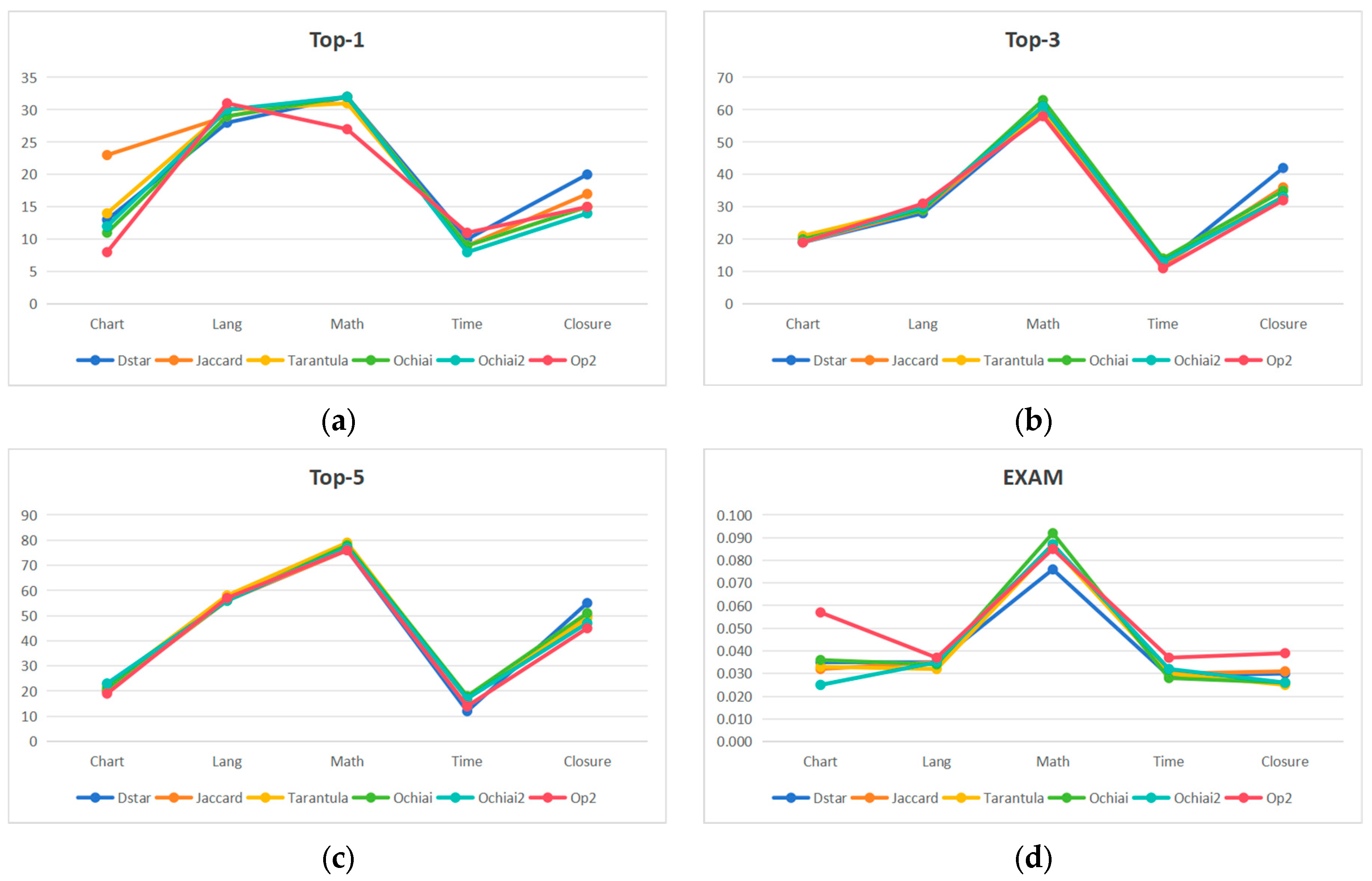
ID	Program	#Faults	LoC	#Tests
Chart	JFreefigure	25	96 k	2205
Closure	Closure Compile	133	90 k	7927
Lang	Apache commons-lang	65	22 k	2245
Math	Apache commons-math	98	81 k	3546
Time	Joda-Time	27	28 k	4130

displays specific information about the Defects4J dataset used. The first column shows the topic IDs that will be used in the remaining text; the second column shows the full names of the projects; the third column shows the number of defects for each project; the forth column shows the latest version’s LoC (Lines of Code) for each project in Defects4J; the fifth column shows the number of test cases each project has.

4.2. Evaluation Metrics

• Top-N

Top-N is an important metric for evaluating the performance of fault localization techniques, with the core being to check whether the actual fault location is accurately included in the top N code locations recommended by the fault localization technique. Specifically, within the Top-N metric framework, these techniques first recommend the Top-N code locations that are most likely to contain faults as candidate areas. Then, the effectiveness of the fault localization technique is assessed by verifying whether faults exist within these candidate areas. In short, it involves calculating how many of the Top-N recommended locations are indeed the actual locations of the faults. Clearly, the larger the value of Top-N, the better the performance of the technique, as it reflects that more accurate fault locations have been successfully identified and included in the Top-N recommended positions.

• EXAM (Expected Additional Mistakes)

EXAM is another commonly used metric for evaluating the performance of fault localization techniques. It is primarily used to measure the percentage of elements that need to be inspected before the actual fault location is found. Specifically, EXAM calculates how many additional elements need to be inspected to find the actual fault location if the fault is not discovered in the Top-N recommended code locations. The formula is as follows:

$$\mathrm{EXAM}={\displaystyle \frac{{\sum }_{i=N+1}^{\left|E\right|}(i-N)·P\left(i\right)}{\left|E\right|-N}}$$

(7)

N is the number of the top N recommended code locations, and E is the set of all possible elements, i.e., the root set. P(i) represents the probability that the i-th element is the fault location; in this paper, P(i) = i/|E|.

5. Results and Analyses

The software fault localization based on the SALSA algorithm proposed in this paper first constructs a Root Set Control Dependency Graph (RSCDG) that contains information on fault propagation. Then, it employs a random walk strategy to analyze the link structure of the RSCDG and scores each node, identifying important nodes related to fault propagation. Each node ultimately has two scores: a hub score and an authority score, which represent the importance and centrality of the faulty statement in the fault propagation process. This paper prioritizes the use of the hub score for the final ranking.

To explore the software localization effects of SA-SBFL, this paper conducted experiments on five projects in Defects4J, using six statistical formulas to calculate the suspicion values of statements as the initial weights of nodes in the RSCDG. The experiments were evaluated from multiple metrics, including Top-1, Top-2, Top-5, and EXAM. To comprehensively verify the effectiveness and practicality of the experiment, this paper evaluates three aspects.

RQ1: How accurate is SA-SBFL in fault localization?

RQ2: Which score is more advantageous in fault localization, the final hub score or the authority score of the node?

RQ3: What are the differences in fault location accuracy when using suspicious values obtained from different statistical formulas such as node weights?

5.1. RQ1: How Accurate Is SA-SBFL in Fault Localization?

Figure 3 demonstrates the fault localization effectiveness of SA-SBFL, traditional SBFL, and TRFL on Top-N (N = 1, 3, 5) across five projects, showing the total number of faults found by each method. It is evident from the figure that SA-SBFL significantly outperforms both traditional SBFL and TRFL in terms of fault localization accuracy, regardless of whether the faulty statements are ranked first, within the top three, or the top five. SA-SBFL exhibits greater precision and reliability in all these cases. The specific localization effects of the three fault localization techniques across the five projects are presented in

Table 5. The fault location results of different technologies in each project.

Project	Technique	Top-1	Top-3	Top-5	EXAM
Chart	SBFL	5	16	19	0.041
	TRFL	12	23	25	0.030
	SA-SBFL	13	21	25	0.031
Closure	SBFL	14	38	39	0.044
	TRFL	22	44	59	0.030
	SA-SBFL	32	65	87	0.025
Lang	SBFL	23	45	55	0.044
	TRFL	31	52	59	0.040
	SA-SBFL	30	54	59	0.040
Math	SBFL	20	56	69	0.102
	TRFL	31	63	79	0.074
	SA-SBFL	32	65	85	0.072
Time	SBFL	6	11	12	0.039
	TRFL	7	12	12	0.033
	SA-SBFL	7	13	14	0.032

. For instance, in the Closure project, SA-SBFL can localize 87 faults on Top-5, which is 48 more than SBFL and 28 more than TRFL. It should also be noted that the statistical formula used by the three methods in the table is Dstar.

Next, let us discuss the performance of SA-SBFL across projects of different complexities. First, according to the Loc and #Tests for each project in Table 4, projects are categorized into low, medium, and high complexity. Closure is considered high complexity, Chart and Math are medium complexity, and Lang and Time are low complexity. From Figure 4, it can be observed that in projects of all complexity levels, SA-SBFL has the lowest EXAM values, while SBFL has the highest EXAM values. Particularly in high-complexity projects, SA-SBFL’s EXAM value is 0.025, which is the lowest among all the techniques. In summary, SA-SBFL demonstrates the highest fault localization accuracy across projects of varying complexities, with its advantage being particularly evident in high-complexity projects.

5.2. RQ2: Which Score Is More Advantageous in Fault Localization, the Final Hub Score or the Authority Score of the Node?

In SA-SBFL, each node ultimately has two scores: the hub score and the authority score. Both of these scores can serve as a basis for fault localization. A high hub score for a node indicates its role in connecting and navigating the link structure, while a high authority score indicates its importance as a source of high-quality information. Therefore, different types of faults are suitable for SA-SBFL to use different scores for fault localization.

Figure 5 illustrates the performance of fault localization using SA-SBFL with both hub scores and authority scores on Top-N (N = 1, 3, 5). The chart shows that on the Top-1 metric, the authority scores on average localized 95 faults across all statistical formulas, while the hub scores-based SA-SBFL localized an average of 97 faults. This indicates that on Top-1, the hub scores perform slightly better than the authority scores. On the Top-3 metric, the authority scores-based SA-SBFL on average localized 185 faults across all statistical formulas, while the hub scores-based SA-SBFL localized an average of 180 faults. This indicates that on Top-3, the authority scores perform slightly better than the hub scores. On the Top-5 metric, the authority scores-based SA-SBFL on average localized 215 faults across all statistical formulas, while the hub scores-based SA-SBFL localized an average of 219 faults. This indicates that on Top-5, the hub scores perform slightly better than the authority scores. In summary, we can see that the performance of the authority scores and hub scores is very close.

Table 6. SA-SBFL (Authority) and SA-SBFL (Hub) fault localization results.

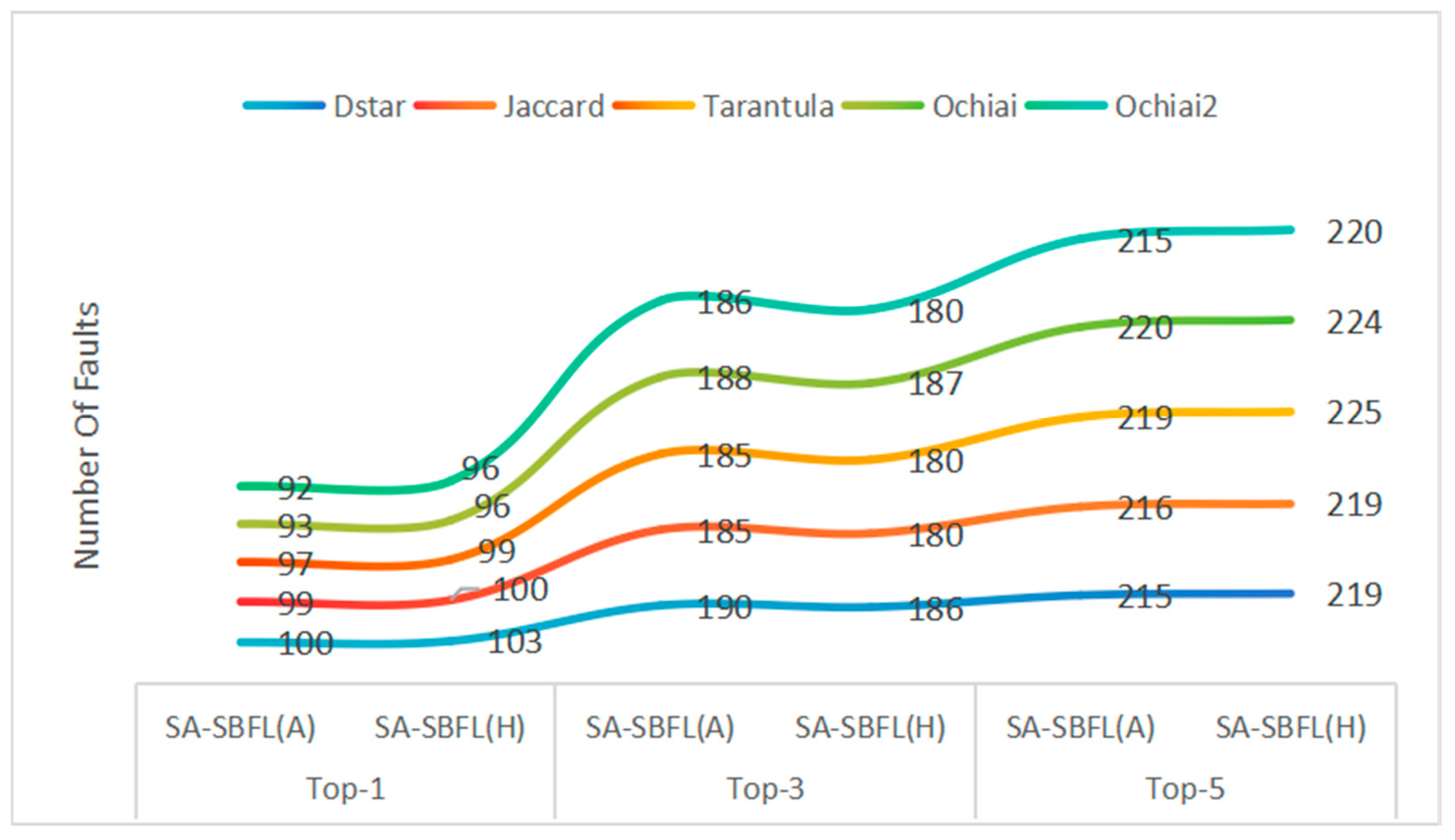
Project	Formula	Top-1		Top-3		Top-5		EXAM
		SA-SBF (A)	SA-SBF (H)	SA-SBF (A)	SA-SBF (H)	SA-SBF (A)	SA-SBF (H)	SA-SBF (A)	SA-SBF (H)
Defects4j	Dstar	100	103	190	186	215	219	0.040	0.041
	Jaccard	99	100	185	180	216	219	0.041	0.043
	Tarantula	97	99	185	180	219	225	0.040	0.041
	Ochiai	93	96	188	187	220	224	0.041	0.043
	Ochiai2	92	96	186	180	215	220	0.039	0.041
	Op2	90	92	180	171	207	211	0.049	0.051

presents the experimental results of SA-SBFL using different scores under six statistical formulas. Hub scores and authority scores each have their advantages under different statistical formulas, and their performance on the Top-1, Top-3, and Top-5 metrics is very close. Although the hub scores slightly outperform the authority scores on Top-1 and Top-5, the authority scores slightly outperform the hub scores in terms of the EXAM value. In summary, in Defects4J, SA-SBFL shows similar fault localization effects when using both authority scores and hub scores. If the type of fault is known, choosing between authority scores or hub scores based on specific circumstances can allow SA-SBFL to locate more faults. Alternatively, combining both scores could further improve the precision of fault localization.

5.3. RQ3: What Are the Differences in Fault Location Accuracy When Using Suspicious Values Obtained from Different Statistical Formulas as Node Weights?

In SA-SBFL, suspicion values calculated through statistical formulas are used as the initial weights of nodes in the RSCDG. However, different statistical formulas weigh the execution of statements in failed and successful test cases, and how they utilize this information to calculate suspicion levels, thus different formulas may perform differently under different types of errors and different distributions of test cases. Similarly, the choice of different statistical formulas will also affect the localization effectiveness of SA-SBFL.

Table 7. Fault localization results of SA-SBFL and SBFL using different statistical formulas.

Project	Technique	Top-1		Top-3		Top-5		EXAM
		SBFL	SA-SBFL	SBFL	SA-SBFL	SBFL	SA-SBFL	SBFL	SA-SBFL	Improvement
Chart	Dstar	5	13	16	19	19	25	0.042	0.035	26.19%
	Jaccard	6	13	17	19	20	24	0.038	0.032	15.79%
	Tarantula	7	14	20	21	22	25	0.037	0.033	10.81%
	Ochiai	6	11	17	20	19	25	0.039	0.036	7.69%
	Ochiai2	6	12	17	19	21	23	0.028	0.025	10.71%
	Op2	5	8	14	19	16	22	0.061	0.057	6.56%
Lang	Dstar	23	28	45	54	55	56	0.044	0.035	20.45%
	Jaccard	22	29	45	53	56	56	0.043	0.035	18.60%
	Tarantula	21	30	45	52	57	58	0.042	0.032	23.81%
	Ochiai	22	29	44	55	56	56	0.043	0.034	20.93%
	Ochiai2	21	30	45	54	55	56	0.042	0.035	16.67%
	Op2	23	31	45	51	56	57	0.046	0.037	19.57%
Math	Dstar	22	32	56	59	69	81	0.102	0.076	25.49%
	Jaccard	22	32	57	60	69	79	0.109	0.087	20.18%
	Tarantula	22	31	57	60	69	79	0.102	0.086	15.69%
Math	Ochiai	22	32	58	63	70	81	0.102	0.092	9.80%
	Ochiai2	22	32	56	61	69	79	0.104	0.087	16.35%
	Op2	21	27	52	58	61	78	0.110	0.085	22.73%
Time	Dstar	6	10	11	12	12	14	0.039	0.029	25.64%
	Jaccard	5	9	9	12	18	17	0.033	0.030	9.09%
	Tarantula	5	9	11	14	16	17	0.032	0.030	6.25%
	Ochiai	6	9	11	14	18	18	0.031	0.028	9.68%
	Ochiai2	5	8	11	13	16	17	0.037	0.032	13.51%
	Op2	8	11	12	11	14	14	0.041	0.037	9.76%
Closure	Dstar	14	20	38	42	39	87	0.044	0.030	31.82%
	Jaccard	13	17	27	36	37	80	0.046	0.031	32.61%
	Tarantula	12	15	26	33	36	79	0.031	0.025	19.35%
	Ochiai	14	15	29	35	39	81	0.037	0.026	29.73%
	Ochiai2	13	14	27	33	37	77	0.036	0.026	27.78%
	Op2	17	15	33	32	42	85	0.053	0.039	26.42%

presents the fault localization effects of SA-SBFL and SBFL using six different statistical formulas.

Figure 6 illustrates the performance of SA-SBFL and traditional SBFL using different statistical formulas in terms of the number of faults localized on Top-N (N = 1, 2, 3) and their performance on the EXAM metric. The chart shows that the Dstar and Tarantula statistical formulas both exhibit lower EXAM values and higher Top-5 values across multiple projects. In particular, Dstar demonstrates consistent performance in the Chart, Lang, and Time projects, while Tarantula stands out in the Lang and Closure projects. Other statistical formulas performed averagely in the experiments. Therefore, this paper concludes that the Dstar and Tarantula statistical formulas are more suitable for application in SA-SBFL.

6. Limitation and Future Work

In the current research on software defect localization, the methodology proposed in this paper has shifted from single-spectrum analysis to a more complex analysis of the linking relationships between program entities, but it still has some obvious limitations. Firstly, the mining of internal program information is not limited to the linking relationships between program entities; it also includes the interactions between program entities in the program execution network. Secondly, this study is constrained by the analysis tools and can only be conducted when the test subject is written in the Java language. This restricts the widespread application of software defect localization techniques. Additionally, the SALSA algorithm used in this paper selects the entire set of program entities executed in failed test cases as the root set, which can lead to a problem where in some cases, the root set is particularly large, resulting in reduced efficiency of defect localization.

In response to these limitations, future research directions could include the following: First, developing defect localization tools that support multiple programming languages. Given the diversity of programming languages, developing a defect localization tool that can adapt to various programming language environments will have broad application prospects. Secondly, exploring more network analysis algorithms that can fully utilize the effective information within the program is possible. Lastly, the selection method for the root set can be optimized to obtain a high-quality root set. Overall, with the increase in software fault localization research and the publication of a large number of related papers, it is expected that more researchers will focus on identifying fault localization issues and providing specific solutions in the future.

7. Conclusions

Fault localization is a critical and complex task in software debugging, especially in manual debugging processes. It not only poses challenges to researchers but also consumes a significant amount of resources. Spectrum-Based Fault Localization (SBFL) technology is a widely discussed method aimed at assisting in the discovery of software defects by analyzing the execution coverage of programs. However, this method does not fully account for the interactions between program entities and data flow, making it difficult to directly translate its analysis results into precise defect locations.

This paper proposes a novel software fault localization method called SA-SBFL, which not only leverages traditional spectrum-based fault localization techniques but also incorporates the SALSA algorithm. By analyzing the linking relationships between program statements and using random walk to identify important program statements within the entire linking network, potential defective program statements are pinpointed. Through this method, a ranking list of the suspiciousness of program statements is ultimately obtained to assist researchers in locating fault positions. To validate the effectiveness of this method, this paper examines five open-source benchmark programs from the Defects4J dataset and compares them with six statistical formulas. The experimental results show that compared to traditional SBFL methods, the method proposed in this paper significantly outperforms traditional SBFL methods, narrowing the code detection scope and thereby enhancing software defect localization performance.

References

- Perscheid, M.; Siegmund, B.; Taeumel, M.; Hirschfeld, R. Studying the advancement in debugging practice of professional software developers. Softw. Qual. J. 2017, 25, 83–110. [Google Scholar] [CrossRef]
- Hailpern, B.; Santhanam, P. Software debugging, testing, and verification. IBM Syst. J. 2002, 41, 4–12. [Google Scholar] [CrossRef]
- Wong, W.E.; Gao, R.; Li, Y.; Abreu, R.; Wotawa, F.; Li, D. Software fault localization: An overview of research, techniques, and tools. In Handbook of Software Fault Localization: Foundations and Advances; Wiley-IEEE Press: Hoboken, NJ, USA, 2023; pp. 1–117. [Google Scholar]
- Abreu, R.; Zoeteweij, P.; Van Gemund, A.J.C. On the accuracy of spectrum-based fault localization. In Proceedings of the Testing: Academic and Industrial Conference Practice and Research Techniques-MUTATION (TAICPART-MUTATION 2007), Windsor, UK, 10–14 September 2007; IEEE: Piscataway, NJ, USA, 2007; pp. 89–98. [Google Scholar]
- Ajibode, A.; Shu, T.; Said, K.; Ding, Z. A fault localization method based on metrics combination. Mathematics 2022, 10, 2425. [Google Scholar] [CrossRef]
- Godboley, S.; Dutta, A.; Mohapatra, D.P.; Mall, R. GECOJAP: A novel source-code preprocessing technique to improve code coverage. Comput. Stand. Interfaces 2018, 55, 27–46. [Google Scholar] [CrossRef]
- Yan, Y.; Jiang, S.; Zhang, Y.; Zhang, S.; Zhang, C. A fault localization approach based on fault propagation context. Inf. Softw. Technol. 2023, 160, 107245. [Google Scholar] [CrossRef]
- Zhao, G.; He, H.; Huang, Y. Fault centrality: Boosting spectrum-based fault localization via local influence calculation. Appl. Intell. 2022, 52, 7113–7135. [Google Scholar] [CrossRef]
- Zhang, Y.; Santelices, R. Prioritized static slicing and its application to fault localization. J. Syst. Softw. 2016, 114, 38–53. [Google Scholar] [CrossRef]
- Hofer, B.; Wotawa, F. Spectrum enhanced dynamic slicing for better fault localization. In ECAI; IOS Press: Amsterdam, The Netherlands, 2012; pp. 420–425. [Google Scholar]
- Qian, J.; Ju, X.; Chen, X. GNet4FL: Effective fault localization via graph convolutional neural network. Autom. Softw. Eng. 2023, 30, 16. [Google Scholar] [CrossRef]
- Ma, Y.F.; Li, M. The flowing nature matters: Feature learning from the control flow graph of source code for bug localization. Mach. Learn. 2022, 111, 853–870. [Google Scholar] [CrossRef]
- Zhang, Z.; Lei, Y.; Mao, X.; Yan, M.; Xia, X.; Lo, D. Context-aware neural fault localization. IEEE Trans. Softw. Eng. 2023, 49, 3939–3954. [Google Scholar] [CrossRef]
- Jones, J.A.; Harrold, M.J. Empirical evaluation of the tarantula automatic fault-localization technique. In Proceedings of the 20th IEEE/ACM international Conference on Automated Software Engineering, Long Beach, CA, USA, 7–11 November 2005; pp. 273–282. [Google Scholar]
- Chen, M.Y.; Kiciman, E.; Fratkin, E.; Fox, A.; Brewer, E. Pinpoint: Problem determination in large, dynamic internet services. In Proceedings of the International Conference on Dependable Systems and Networks, Washington, DC, USA, 23–26 June 2002; IEEE: Piscataway, NJ, USA, 2002; pp. 595–604. [Google Scholar]
- Abreu, R.; Zoeteweij, P.; Golsteijn, R.; Van Gemund, A.J. A practical evaluation of spectrum-based fault localization. J. Syst. Softw. 2009, 82, 1780–1792. [Google Scholar] [CrossRef]
- Naish, L.; Lee, H.J.; Ramamohanarao, K. A model for spectra-based software diagnosis. ACM Trans. Softw. Eng. Methodol. 2011, 20, 1–32. [Google Scholar] [CrossRef]
- Wong, W.E.; Debroy, V.; Gao, R.; Li, Y. The DStar method for effective software fault localization. IEEE Trans. Reliab. 2013, 63, 290–308. [Google Scholar] [CrossRef]
- Yoo, S.; Xie, X.; Kuo, F.C.; Chen, T.Y.; Harman, M. No pot of gold at the end of program spectrum rainbow: Greatest risk evaluation formula does not exist. RN 2014, 14, 14. [Google Scholar]
- de Souza, H.A.; Mutti, D.; Chaim, M.L.; Kon, F. Contextualizing spectrum-based fault localization. Inf. Softw. Technol. 2018, 94, 245–261. [Google Scholar] [CrossRef]
- He, H.; Ren, J.; Zhao, G.; He, H. Enhancing spectrum-based fault localization using fault influence propagation. IEEE Access 2020, 8, 18497–18513. [Google Scholar] [CrossRef]
- Fan, X.; Wu, K.; Zhang, S.; Yu, L.; Zheng, W.; Ge, Y. Fault Localization Using TrustRank Algorithm. Appl. Sci. 2023, 13, 12344. [Google Scholar] [CrossRef]
- Yan, Y.; Jiang, S.; Zhang, Y.; Zhang, C. An effective fault localization approach based on PageRank and mutation analysis. J. Syst. Softw. 2023, 204, 111799. [Google Scholar] [CrossRef]
- Zhang, M.; Li, X.; Zhang, L.; Khurshid, S. Boosting spectrum-based fault localization using pagerank. In Proceedings of the 26th ACM SIGSOFT International Symposium on Software Testing and Analysis, Santa Barbara, CA, USA, 10–14 July 2017; pp. 261–272. [Google Scholar]
- Podgurski, A.; Clarke, L. The implications of program dependencies for software testing, debugging, and maintenance. In Proceedings of the ACM SIGSOFT’89 Third Symposium on Software Testing, Analysis, and Verification, Key West, FL, USA, 13–15 December 1989; pp. 168–178. [Google Scholar]
- Harrold, M.J.; Offutt, A.J.; Tewary, K. An approach to fault modeling and fault seeding using the program dependence graph. J. Syst. Softw. 1997, 36, 273–295. [Google Scholar] [CrossRef]