Enhancing Indoor Localization with Room-to-Room Transition Time: A Multi-Dataset Study

Abstract

With the rapid advancement of network technologies and the widespread adoption of smart devices, the demand for efficient indoor localization and navigation systems has surged. Addressing the navigation challenge without requiring additional hardware is critical for the broad adoption of such technologies. Among various fingerprint-based systems—such as Bluetooth, ZigBee, or FM radio—Wi-Fi-based indoor positioning stands out as a practical solution, due to the pervasiveness of Wi-Fi infrastructure in public indoor spaces. This study introduces an ESP32-based data-collection tool designed to minimize offline training time for Wi-Fi fingerprinting, and it presents a novel dataset incorporating room-to-room transition time, which represents the time taken to move between rooms, alongside Wi-Fi signal strength data. The proposed approach focuses on room-level localization, leveraging Machine Learning (ML) models to predict the most likely room rather than precise (x, y) coordinates. To assess the effectiveness of this feature, three datasets were collected from different residential environments by three different individuals, enabling a comprehensive evaluation across multiple spatial layouts and movement patterns. The experimental results demonstrate that incorporating room-to-room transition time consistently enhanced localization performance across all the datasets, with accuracy improvements ranging from 1.17% to 12.47%, depending on the model and dataset. Notably, the Wide Neural Network model exhibited the highest improvement, achieving an accuracy increase from 82.37% to 94.77%, while the Ensemble-based methods such as Ensemble Bagged Trees also benefited significantly, reaching up to 93.17% accuracy. Despite varying gains across the datasets, the results confirm that integrating room-to-room transition time improves Wi-Fi-based indoor positioning by leveraging temporal movement patterns to enhance classification.

1. Introduction

The rapid advancement of wireless network technologies has received significant interest in the practical application of location-based services for both indoor and outdoor environments. While GPS-based localization services are extensively used outdoors with high accuracy, their efficacy indoors is compromised, due to obstructions like walls and doors leading to weak signal reception [1]. Hence, alternative methods, such as fingerprinting [2,3], triangulation [4], trilateration [4], proximity [5], and pedestrian dead reckoning [6] are utilized for indoor environments [7]. Compared to other methods, fingerprinting-based techniques require less hardware, and they are capable of performing localization and navigation using signal strength values from various wireless network technologies, such as FM radio [8], Wi-Fi [9], Bluetooth [10], Radio Frequency Identification Device (RFID) [11], Ultra Wide Band (UWB) [12], and ZigBEE [13]. Among these technologies, Wi-Fi fingerprint-based applications are widely used in public areas, such as museums, shopping malls, and parking lots, so positioning can be done with these services using only a mobile device without the cost of additional hardware. While alternatives, such as UWB and BLE, have higher sensitivity and efficiency, the need for infrastructure makes their widespread use in specific scenarios impractical. As another alternative, although FM radio is widespread and offers wide coverage, its application for fine-grained indoor localization is limited [14]. FM signals are typically designed for long-range communication and are not optimized to capture the small-scale spatial variations required to distinguish closely located indoor spaces. The relatively low frequency of FM signals results in larger wavelengths that are less sensitive to obstacles and environmental changes that are critical for room-level discrimination in indoor environments [15]. Wireless Local Area Networks (WLANs), on the other hand, operate at higher frequencies and provide rich spatial diversity, making them more suitable for precise indoor localization [16].

Wi-Fi is a wireless communication technology employed in WLAN, and it generally operates in the frequency range between 2.4 GHz and 5.8 GHz [17,18]. Current Wi-Fi technology does not provide direct information about the distance between the access point and the signal receiver, but the Wi-Fi signal strength level indicates the distance and proximity of the signal receiver to the access point. The Basic Service Set Identifier (BSSID), which is a unique identifier, is used to obtain information about the MAC address associated with the Wi-Fi signal strength [19]. In this context, the signal strengths corresponding to each BSSID were taken into account in our study.

In Wi-Fi-based fingerprinting methods for indoor localization, an offline radio map is first generated by collecting Received Signal Strength Indicator (RSSI) data from the target environments. During the online phase, the real-time location of the target device is estimated by leveraging previously measured RSSI data. In this study, a sensor fusion approach is proposed by integrating Wi-Fi signals with room-to-room transition time, which represents the time taken to move from one room to another, measured using the mobile device clock as a sensor. This feature is incorporated into Wi-Fi-based fingerprinting systems to enhance room-level localization accuracy by utilizing ML models.

This study builds upon our preliminary work [20], which proposed room-to-room transition time as a novel feature for indoor localization. While the previous study introduced the concept, it was limited to a single dataset and a narrower experimental setup. In this work, we expand the evaluation by testing the feature across multiple datasets from different residential environments and systematically analyzing its impact on classification performance, using a broader range of ML models. The experimental results demonstrate that the inclusion of room-to-room transition time consistently improves localization accuracy across diverse settings, reinforcing its general applicability. In summary, the contributions of this study are listed below:

• The general applicability of the room-to-room transition time feature was validated through experiments conducted on multiple datasets collected from different residential environments, demonstrating its robustness across varying spatial layouts and user movement patterns.
• A diverse set of ML algorithms, including Ensemble methods and Neural Networks, was employed to systematically evaluate the impact of the proposed feature on indoor localization performance.
• An ESP32-based data-collection system has been developed to automate the acquisition of Wi-Fi signal fingerprints, streamlining the data-collection process and enhancing consistency in training data.
• A set of high-quality datasets, incorporating Wi-Fi fingerprints and room-to-room transition times, is introduced to support further research in fingerprinting-based indoor localization.

2. Related Work

In recent years, indoor positioning applications, which have attracted attention both in academia and industry, have offered solutions to many problems, such as target tracking, inventory management, room-level location, and machine fault detection [21]. Since GPS sensors cannot be used in indoor positioning, due to signal fading, various sensors are used to ensure accuracy and reliability [22]. Although there are many positioning systems associated with modern technology today, these systems aim to minimize positioning error, since systems with low cost and without the use of any special devices are preferred. Indoor positioning methods can be divided into two groups: “special sensor systems” and “ambient sensor systems” [23]. Although the development of special sensor systems and placement of these systems in the environment or on the human body have advantages, such as minimizing the position estimation error, they also have disadvantages, such as installation and hardware costs, user adaptation to the new system, and the need for installation whenever the user needs it. Ambient sensor systems, on the other hand, are more suitable for individual and general-purpose use as they do not require installation costs and additional hardware, and they are also available on devices (smartphones, tablets, etc.) that the user can carry at any time [24]. For this reason, in order to achieve indoor positioning accuracy at minimum cost, there are various studies in the literature that generally use the existing sensors of the smartphones [25,26,27,28,29,30,31,32,33]. Among these studies, WLAN, Wi-Fi, BLE, and FM radio are used as wireless signals for fingerprint-based indoor positioning. The RSSIs of these signals are called fingerprints and are given as features to artificial intelligence models. In addition to RSSI, other features, such as Channel Impulse Response (CIR) and Channel State Information (CSI), can be used. Flexible and easy to deploy, fingerprint-based systems are considered as potential solutions for cost-effective indoor localization. In addition to the Wi-Fi and Bluetooth sensors of the smartphone, various sensors, such as accelerometer, magnetometer, barometer, light, and gyroscope, are used to extract features [33,34]. Although various signal strengths received from the different sensors are used as a feature, to the best of our knowledge the use of transition time information between rooms has not been encountered, except in our previous study [20]. In a study similar to the calculation of room–room transition time, Zhu et al. [35] analyzed the spatial geometric distribution, time sequence, and statistical features within different sliding windows from Global Navigation Satellite System (GNSS) measurements on smartphones, to estimate the Indoor/Outdoor (IO) times between indoor and outdoor transitions with high accuracy. After this feature-extraction process, they proposed a new high-accuracy IO detection model by calculating the detection result with the Hidden Markov Model (HMM), using an Ensemble model based on stacking and filtering. In their experimental results, up to 94.53% accuracy of IO transition detection was achieved.

Table 1. Feature and method comparisons of the proposed approach and state-of-the-art studies (LSTM: Long Short-Term Memory, RNN: Recurrent Neural Network, CNN: Convolutional Neural Network, SVM: Support Vector Machine, k-NN: k-Nearest Neighbor, MLA-MFL: Map Location Anchors with Multisensor Fusion Location, HMM: Hidden Markov Model).

Study	Sensors	Feature Types	Methods	Accuracy
Wang et al. [36]	magnetic, light sensors	fusion of magnetic field data and light intensity data	LSTM	mean error: 1.39 m
Zhou et al. [32]	accelerometer, gyroscope, gravimeter, magnetometer	signal fusion	RNN, CNN	RMSE < 1.2 m
Yan et al. [30]	Bluetooth, Wi-Fi, inertial camera	LTE signal, Bluetooth, camera image, Wi-Fi radio image	SVM, CNN	region (92%)
Lamoureux and Chelouah [37]	magnetometer, gyroscope	magnetic fields, iBeacon radio, RSSI	k-NN	RMSE: 1.4 m
Li et al. [27]	Wi-Fi, magnetometer	CSI and magnetic field strength	Multi Module Data k-NN	avg error < 0.5 m
Jianhua et al. [33]	Bluetooth, accelerometer, gyroscope, barometer, magnetometer	signal fusion	MLA-MFL	avg error: 0.72 m
Zhu et al. [35]	GNSS	spatial geometry distribution, time sequence, and statistical features of GNSS measurement	stacking model with HMM	94.53–92.80%
This study	ESP32 Wi-Fi module and clock time of smartphone	RSSI and room-to-room transition time	Wide Neural Network	room-level (94.7%)

summarizes the sensors, features, and classification methods used in fingerprint-based indoor positioning studies in the literature. In our previous study [20], Wi-Fi signals were collected manually, using a mobile application. A key distinction in this study was the automation of the data-collection process through a hardware setup, eliminating the need for manual collection. Additionally, the dataset was expanded, and better performance was achieved by incorporating Ensemble and Regression-based methods alongside traditional ML techniques.

3. Material and Method

The proposed fingerprint-based indoor positioning method was divided into two phases: offline (data collection) and online (test). In the offline phase, a hardware setup and a mobile application were used to collect Wi-Fi signal strengths and room-to-room transition times, respectively, across three different residential environments. The floor plan shown in Figure 1 corresponds to the house used in Dataset 2, while additional datasets were collected in two other houses with distinct spatial layouts. In the online phase, different ML models were trained and tested using these datasets, which contained Wi-Fi signal strengths and transition times between rooms. These phases are explained in the following subsections.

The proposed system is based on active localization, as it relies on the use of wireless devices such as a smartphone and ESP32 module in the offline phase for localization. Passive or device-free localization systems differ from active localization systems in terms of practicality and scalability as they incur higher infrastructure costs, such as the use of Radio Frequency (RF) sensing (e.g., Wi-Fi Channel State Information [CSI]), vision-based systems, infrared sensors, or Light Spectral Information (LSI) [38,39,40,41,42].

3.1. Offline (Data-Collection) Phase

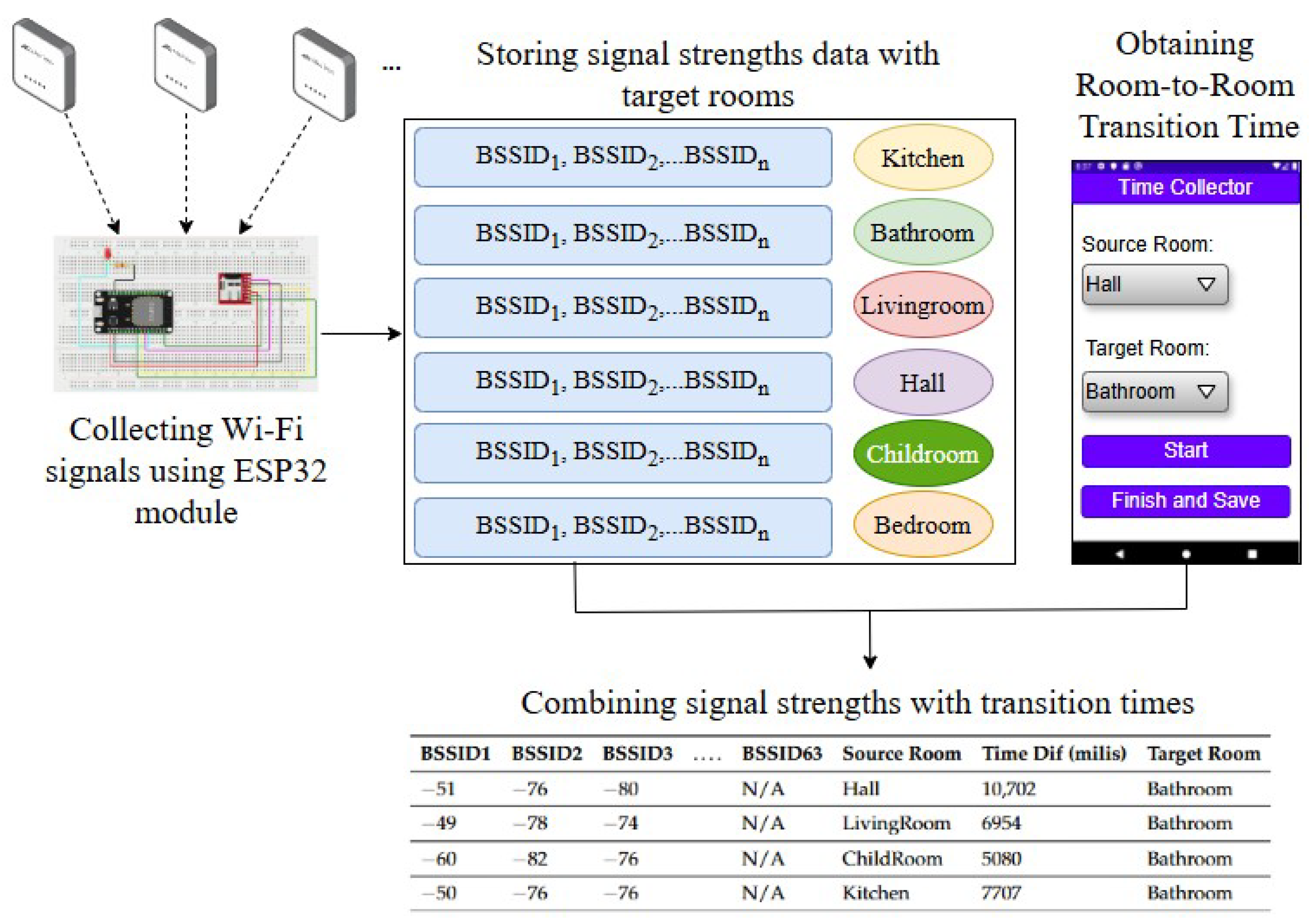
For this phase, two distinct data-collection methods were developed: hardware setup and mobile application. While hardware setup was used to collect large numbers of Wi-Fi signal strengths, the mobile application was used to obtain room-to-room transition time when the user was walking between rooms. The data obtained were combined for further processing in the online phases. The data-collection process is shown in Figure 2. The design and implementation details of each data-collection method are discussed below.

3.1.1. Hardware Setup for Automated Wi-Fi Data Collection

To measure Wi-Fi signal strength, a hardware setup comprising an ESP32-DevKitC (ESP32) module [43], a MicroSD card module, and a portable power bank was employed. The ESP32-based Wi-Fi signal-collection module was assembled on a breadboard and strategically positioned at predetermined fixed locations within each room. This module was programmed to record Wi-Fi signal strength at 5 min intervals, storing the data on the MicroSD card. Over a single session, this configuration facilitated the collection of up to 500 data points per room, allowing for continuous data collection for approximately 41.6 h (around two days). This setup ensured efficient and automated data acquisition, reducing manual intervention and maintaining high reliability in signal strength measurement.

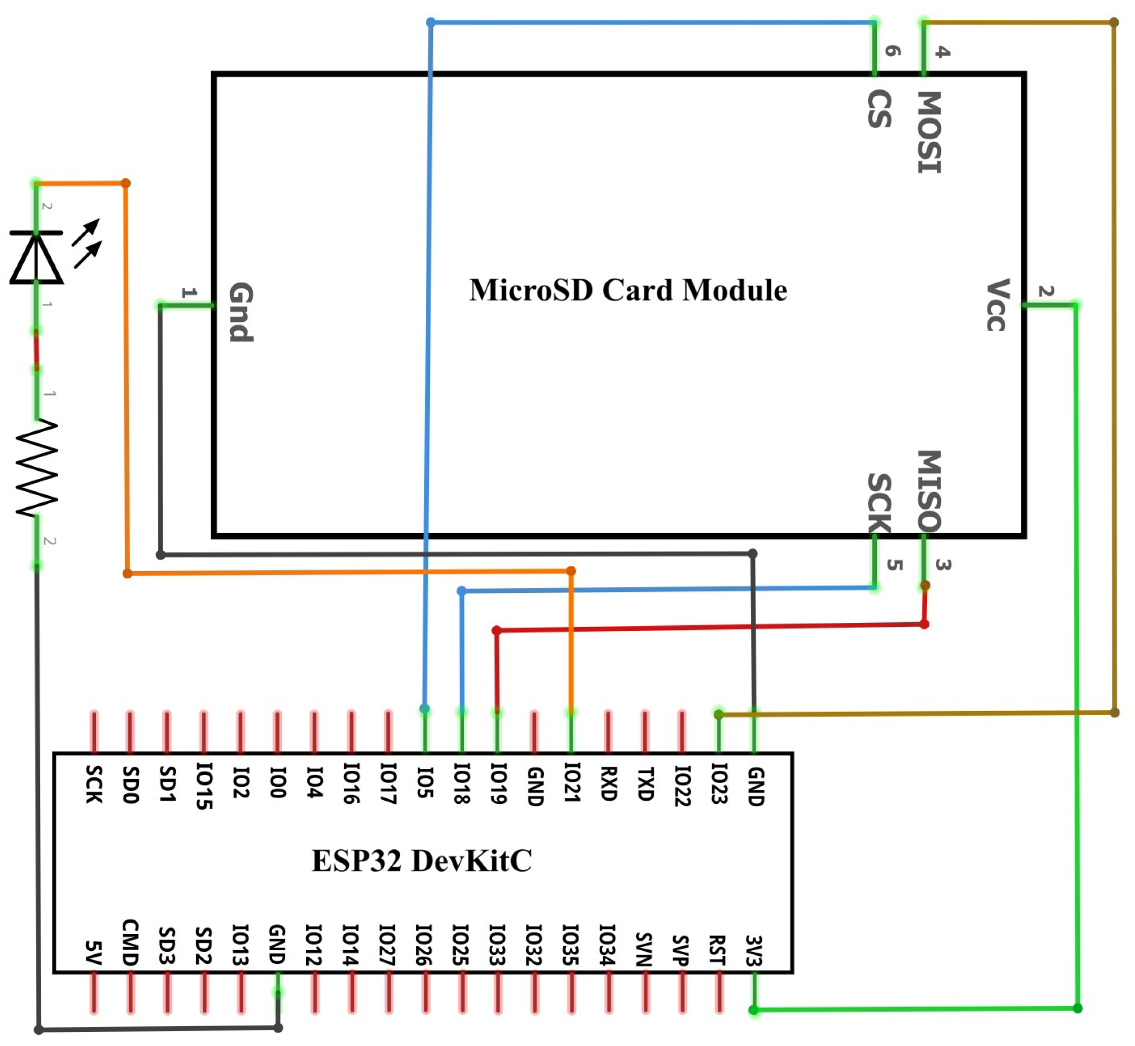
The circuit diagram of the hardware setup is shown in Figure 3. The ESP32 development board [43] featured a dual-core Xtensa® 32-bit LX6 processor running at 240 MHz and 520 kilobytes of Static Random-Access Memory (SRAM), along with integrated Wi-Fi and Bluetooth modules. The development board was connected to an external SD card module via the Serial Peripheral Interface (SPI) for data logging.

To maintain uninterrupted operation, the study utilized two power banks in an alternating manner. While one power bank powered the ESP32 module during data collection, the other was recharged, ensuring continuous functionality. The ESP32 module was programmed to signal the completion of data collection via a blinking red LED indicator. Upon activation of the indicator, the device was disconnected from the power source, and the collected data, stored in CSV format on the SD card, were transferred to a computer for subsequent processing.

Following the data-collection phase, three raw datasets were generated, each corresponding to a different residential environment. In total, 3000 data points were collected for each dataset. Dataset 1 contained 58 unique BSSIDs, Dataset 2 included 63 unique BSSIDs, and Dataset 3 comprised 41 unique BSSIDs, reflecting the variations in Wi-Fi signal availability across different environments.

3.1.2. Mobile-Based Data Collector for Room Transition Time Measurement

A mobile application was developed to measure the time it took a user to move from one room (source) to another (target) in milliseconds. When the user started moving, he/she pressed the “Start” button to start the time measurement, and when he/she reached the target room, he/she pressed the “Finish” button to record the transition time between the two rooms. The first author of the study took part in collecting data at a daily walking speed.

The Wi-Fi signals obtained from the hardware setup and the room-to-room transition times collected via the mobile application were combined in three different datasets, to assess the general applicability of room-to-room transition time.

Table 2. A sample (from Dataset 2) of the combined Wi-Fi and Room-to-Room Time Difference datasets (N/A: Not Available).

BSSID1	BSSID2	BSSID3	….	BSSID63	Source Room	Time Dif (milis)	Target Room
−51	−76	−80		N/A	Hall	10,702	Bathroom
−49	−78	−74		N/A	LivingRoom	6954	Bathroom
−60	−82	−76		N/A	ChildRoom	5080	Bathroom
−50	−76	−76		N/A	Kitchen	7707	Bathroom
−51	−82	−89		N/A	Bedroom	7156	Bathroom
−77	−93	−84		−91	Kitchen	12,278	Bedroom
−75	−91	−83		−92	Bathroom	6596	Bedroom
−76	−91	−85		−92	LivingRoom	9976	Bedroom
−73	−89	−86		−90	Hall	10,960	Bedroom
−75	−90	−84		−88	ChildRoom	6832	Bedroom
−68	N/A	−81		N/A	Hall	8872	Kitchen
−67	−87	−81		N/A	Bathroom	7904	Kitchen
−68	−87	−81		N/A	LivingRoom	8456	Kitchen
−68	−85	−80		N/A	ChildRoom	9954	Kitchen
−67	−86	−82		N/A	Bedroom	11,306	Kitchen
N/A	−77	N/A		N/A	ChildRoom	8409	LivingRoom
N/A	−80	N/A		N/A	Bedroom	10,482	LivingRoom
N/A	−81	N/A		N/A	Bathroom	6700	LivingRoom
N/A	−79	N/A		N/A	Kitchen	8458	LivingRoom
N/A	−80	N/A		N/A	Hall	8221	LivingRoom
−66	−88	N/A		N/A	Bathroom	8063	Hall
−67	−90	N/A		N/A	Bedroom	11,471	Hall
−68	−88	N/A		N/A	Kitchen	7470	Hall
−66	−89	N/A		N/A	ChildRoom	9049	Hall
−68	−90	N/A		N/A	LivingRoom	7483	Hall
−44	−93	−71		N/A	Hall	9932	ChildRoom
−43	−89	−69		N/A	LivingRoom	8142	ChildRoom
−43	−95	−79		N/A	Kitchen	9068	ChildRoom
−44	−89	−69		N/A	Bathroom	4653	ChildRoom
−44	−95	−77		N/A	Bedroom	7319	ChildRoom

presents a sample from Dataset 2.

When the values given in Table 2 were examined, the BSSID measurements were the expression of the signal strengths of the access points obtained as dBm format. If no signal was received from the BSSID, it was recorded as 0 dbm in the dataset. These values are expressed as Not Available (N/A) in Table 2. In addition, the time elapsed during the transition from a source room to a target room was recorded in the dataset as an instantaneous time difference feature.

Table 3. Summary of the datasets used in this study, including house sizes and the demographic characteristics of the data collectors (gender, age, and height).

Dataset	House Size (m2)	Collector
		Gender	Age	Height (cm)
Dataset 1	195	Female	30	163
Dataset 2	145	Female	34	162
Dataset 3	130	Male	45	182

summarizes the key characteristics of the three datasets used in this study. Each dataset was collected in a different residential environment with varying spatial layouts and by individuals with different characteristics, such as height, age, and gender. The house sizes ranged from 130 m² to 195 m², while the data collectors varied in gender, age, and height, which may have introduced additional variability in walking patterns and transition times. This table provides an overview of these differences, supporting the generalizability of the room-to-room transition time analysis.

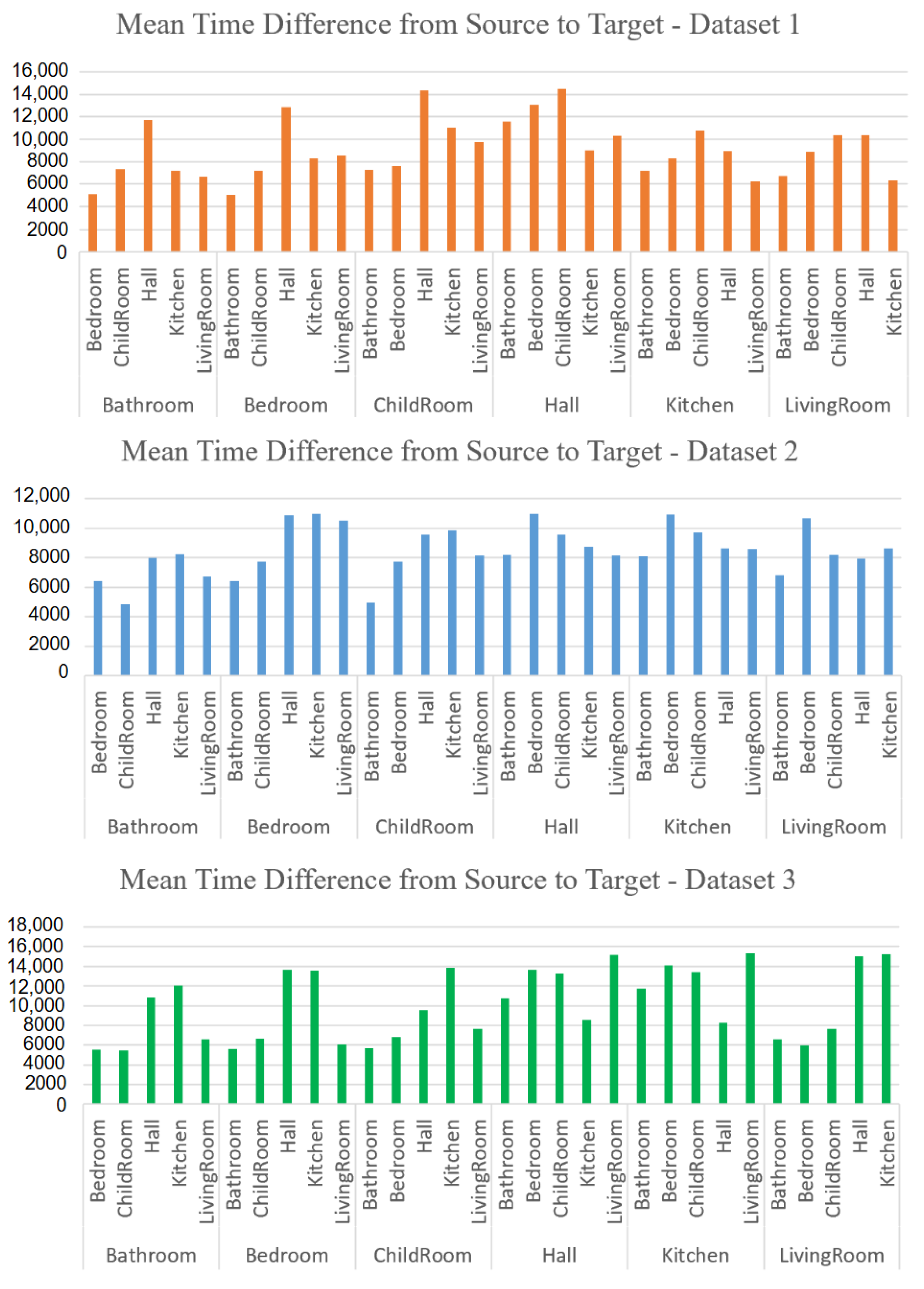
Figure 4 shows the mean transition times between the source and target rooms across the three datasets. As an example, in Dataset 2 the mean time difference from the Bathroom to the Bedroom, which were close to each other, was 6414 ms, while the average time difference from the Bathroom to the Kitchen, which were farther apart, was 8008 ms. The data collector walked at a natural pace during the different time periods, and the transition times varied, based not only on the distance between rooms but also on the collector’s physical condition and mental state at the time of the data collection.

Table 4. Approximate distances (in cm) and estimated step counts between room pairs for each dataset. Distances were measured as accurately as possible, using a measuring tape, considering pathway curvatures. Step counts were estimated based on a sample walking path between rooms.

Room Pair	Dataset 1		Dataset 2		Dataset 3
	Distance	Steps	Distance	Steps	Distance	Steps
Kitchen–Livingroom	895	13	797	11	1210	23
Kitchen–Bedroom	1090	18	1066	15	1095	21
Kitchen–Hall	777	13	930	15	680	14
Kitchen–Bathroom	790	13	876	13	975	18
Bathroom–Bedroom	640	9	545	8	420	9
Bathroom–Hall	705	12	1153	19	885	17
Livingroom–Bedroom	1055	16	934	14	430	9
Livingroom–Bathroom	750	11	708	12	530	11
Livingroom–Hall	767	11	1073	17	1140	22
Bedroom–Hall	1062	17	1254	22	1150	22
Childroom–Livingroom	900	14	1133	16	580	12
Childroom–Bathroom	450	7	732	11	400	8
Childroom–Bedroom	790	13	693	11	430	9
Childroom–Kitchen	1007	16	1183	18	1040	20
Childroom–Hall	935	15	1482	24	1030	20

presents the approximate distances and corresponding step counts between rooms, providing an overview of the spatial relationships within the different residential environments. To ensure the accuracy of the distance measurements between the rooms, a measuring tape was used, and the paths were divided into smaller segments, to account for possible curvatures. The step count was estimated based on a representative walking path between rooms, reflecting typical movement patterns.

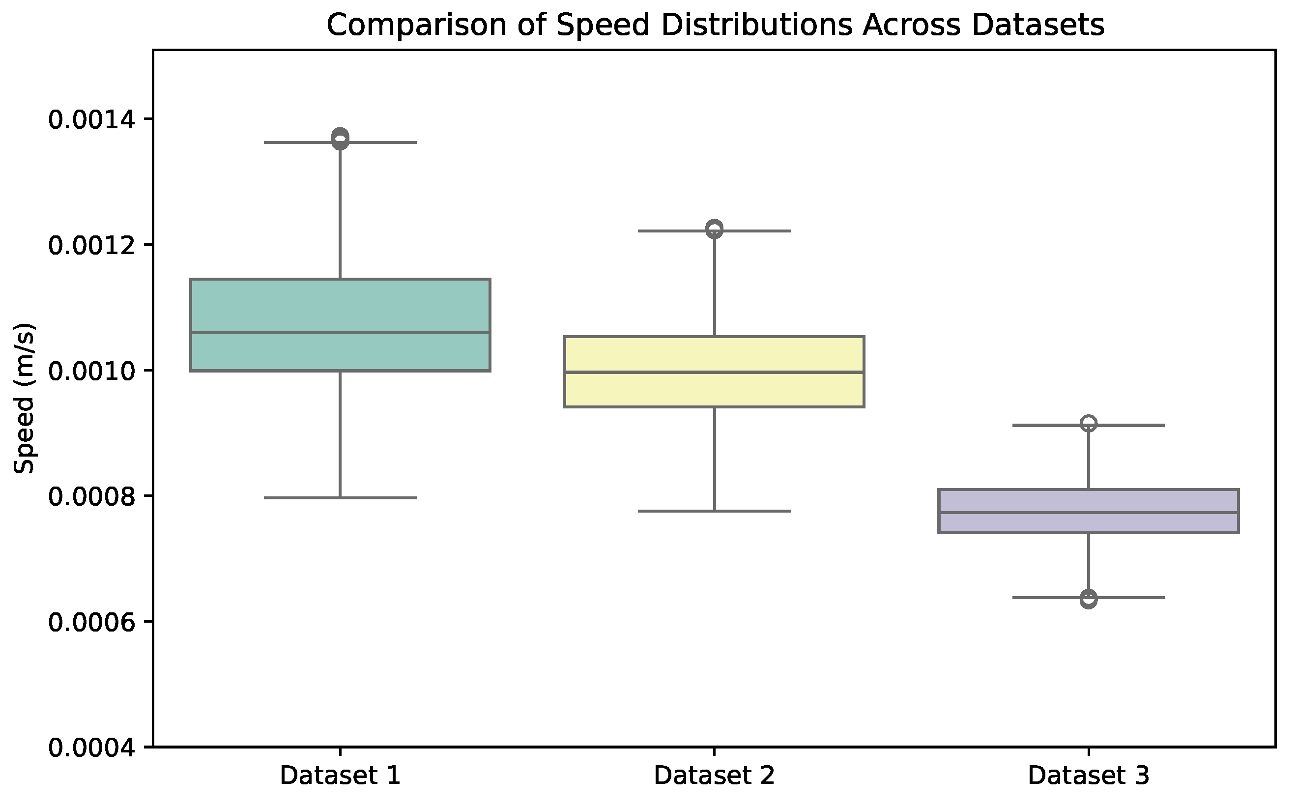
The average speeds calculated using the room-to-room transition data from the datasets are presented in Figure 5. The walking speed for each transition was obtained by dividing the approximate distance between rooms by the recorded transition time. While Figure 5 indicates that the walking speeds varied across different room pairs, Figure 6 shows that when the speeds were aggregated at the dataset level there were noticeable differences between the datasets. This suggests that both spatial-layout and individual-movement characteristics contributed to the observed variations in walking speed across the different home environments.

3.2. Online (Learning-and-Test) Phase

During the online phase, both the raw dataset and the combined datasets, which integrated the Wi-Fi signal strengths with the room-to-room transition times, were utilized to train various ML models for accurately predicting target rooms. The flowchart describing the online phase is shown in Figure 7.

In Figure 7, both the BSSID names received from the ESP32 microcontroller for each target room and the signal strengths corresponding to these BSSIDs were recorded for certain periods of time, and the target room was added to the dataset as a label. In addition to the Wi-Fi signal strengths, a mobile application was developed to calculate the transition time of the user from one room (source room) to another room (target room) and, as a result, Wi-Fi signal strengths, source room, time difference, and target room information were used to classify the target room. In the online phase, the raw Wi-Fi dataset and the Wi-Fi+Room-to-Room Transition Time datasets obtained in the offline phase were divided into training and test sets by 10-fold cross-validation. Then, various supervised ML algorithms were used to train the dataset, and the prediction models obtained from the training phase were used to predict the target room information, using the BSSID signals and transition times in the test set.

Then, the effect of the transition time between rooms on the classification performance was analyzed. This dataset of labeled locations was used in the test phase to model the relationship between fingerprints and location, in order to estimate the location of an unknown fingerprint. In this study, 34 supervised learning algorithms were implemented, including Classification Trees (Fine Tree, Coarse Tree, Medium Tree), Discriminant Analysis (Quadratic, Linear), Naive Bayes, Nearest Neighbors (Fine, Medium, Cosine, Weighted), Support Vector Machine (Linear, Quadratic, Cubic, Medium Gaussian, Coarse Gaussian), Classification Ensembles, and Neural Networks (Narrow, RusBoosted, Bilayered, Trilayered). To determine which algorithms to retain for further analysis, the highest-performing algorithm within each model category (e.g., SVM, k-NN, Decision Trees) was selected. Instead of applying a strict accuracy threshold, the best-performing model from each category was chosen, based on its ability to achieve the highest accuracy while maintaining computational efficiency. This approach ensured that the most effective algorithms, based on their predictive accuracy, were included in the subsequent analysis while less performant models were excluded.

Among the supervised learning algorithms, Fine Tree (a variant of Decision Tree Classifiers), Efficient Logistic Regression, Weighted K-Nearest Neighbors (k-NN), Linear Support Vector Machine (SVM), Wide Neural Network, and Ensemble Bagged Trees yielded the most promising results and were subsequently compared across both datasets. In the following subsections, each method is described according to its characteristics.

3.2.1. Fine Tree

Fine Tree [44], one of the Decision Tree classification models, optimizes the structure of the Decision Tree by employing preprocessing methods, such as pruning and removing unnecessary branches and nodes, thereby reducing overfitting and balancing model complexity through parameter adjustments [45]. It aims to improve accuracy by combining the predictions generated by multiple trees using Ensemble methods [46]. Additionally, by applying regularization [47] to control overfitting and enhance the model’s generalization ability, Fine Tree helps Decision Tree classifiers achieve better results in data prediction tasks.

3.2.2. Linear Discriminant Analysis

Linear Discriminant Analysis (LDA) [48] is a well-established dimensionality reduction technique primarily used for classification tasks. It aims to maximize the separation between different classes by projecting the data onto a lower-dimensional space where class distinctions are most prominent. This is achieved by computing the between-class variance, which captures the spread of different class means, and the within-class variance, which accounts for variations within each class. The optimal projection is found by solving the eigenvalue problem for the matrix that balances these variances, ensuring that data points from the same class are close together while those from different classes are well-separated. LDA is widely used in applications such as pattern recognition, face recognition, and medical diagnostics, though it has limitations when dealing with non-linearly separable classes or small sample sizes, requiring modifications such as kernel LDA or regularized LDA.

3.2.3. Efficient Logistic Regression

Efficient Logistic Regression [49] operates faster and more scalably compared to traditional Logistic Regression methods, even on larger-scale datasets. Efficient Logistic Regression utilizes the fitclinear function for binary-class data and the fitcecoc function for multi-class data [50]. These functions enable the model to train on datasets with a large number of observations by significantly reducing training computation time compared to traditional Logistic Regression models. Specifically, it employs various optimization techniques to shorten training times for large datasets.

3.2.4. Weighted k-NN

Weighted k-Nearest Neighbors (Weighted k-NN) [51] is a weighted model of the k-Nearest Neighbors (k-NN) algorithm. In this model, each neighbor’s influence on the prediction is weighted based on its distance. Closer neighbors have more weight in the prediction. Weights are usually calculated using inverse distance or a similar formula. Weighted k-NN provides more accurate predictions by calculating the contributions of different neighbors based on distance, rather than equally. This model is particularly useful when the differences between the effects of data points are significant.

3.2.5. Cosine k-NN

Cosine k-NN [52] is founded on the assessment of angular similarity between two vectors in a multidimensional space, as opposed to their absolute magnitudes. This method utilizes cosine similarity as the distance metric, distinguishing it from the traditional k-NN algorithm, which relies on Euclidean distance. By focusing on the directional alignment of vectors, Cosine k-NN is particularly effective in capturing relationships in high-dimensional and sparse data.

3.2.6. Coarse k-NN

Coarse k-NN [53] is a variant of KNN where the number of neighbors is kept larger. This method attempts to capture general trends by increasing the number of near neighbors to create a wider decision boundary. Considering more neighbors allows the model to classify based on general patterns rather than individual instances. However, this can lead to ignoring detailed local variations and reduce the classification sensitivity of the model. Coarse KNN is less sensitive to small changes in the data and is suitable for identifying larger-scale trends. However, it also has disadvantages, such as increased complexity and less precise decision boundaries.

3.2.7. Linear SVM

Linear SVM (Linear Support Vector Machine) [54] is an ML model for classification on a linearly separable dataset. Its main purpose is to classify data points into two classes by creating a decision boundary between two different classes. Linear SVM aims to achieve the maximum margin (distance) when building the delimiter. This means finding the widest gap between the two classes. The marginal classification objective increases the ability to accurately classify new observations and generally improves the generalization ability of the model.

3.2.8. Medium Gaussian SVM

Medium Gaussian SVM [55] is a robust ML algorithm designed for high-accuracy classification of non-linear datasets. It leverages the Gaussian Radial Basis Function (RBF) kernel to enhance classification performance by mapping input data into a higher-dimensional space. Unlike the standard SVM, Medium Gaussian SVM employs a moderate gamma parameter, striking a balance between decision boundary flexibility and model complexity. This adjustment mitigates the risk of overfitting, thereby improving the model’s generalization capability. By identifying a subset of the training data as support vectors, the algorithm constructs an optimal hyperplane for classification. The use of the Gaussian kernel enables effective handling of datasets that are not linearly separable, making it particularly suitable for complex pattern-recognition tasks.

3.2.9. Wide Neural Network

A Wide Neural Network [56] is a structure in artificial neural network architecture that usually contains a large number of neurons in the input layer. This model is used to learn complex relationships between many features. A Wide Neural Network can represent a large feature space, to capture different combinations of input data. This is especially useful when working with high-dimensional and large-scale datasets, because it can model more complex relationships using more parameters and layers. Thus, it allows for more effective feature extraction and learning of more complex data structures in a larger feature space. This model is especially used in problems where there are non-linear relationships between features, and it is often preferred for representing high-dimensional datasets.

3.2.10. Ensemble Bagged Trees

Ensemble Bagged Trees [57] is an Ensemble method that combines many Decision Trees to form a powerful classification or Regression model. Using the Bagging (Bootstrap Aggregating) technique, random samples are generated from the dataset and separate trees are trained on each sample. Then, the predictions of these trees are averaged or modulated to make the final prediction. This method compensates for the errors of a single tree, increases generalization ability, and reduces overfitting. Ensemble Bagged Trees are known for their robustness and ability to learn complex relationships. Bagging reduces variance by training each tree on different samples, while reducing bias by aggregating the trees [58]. For this reason, the model ensures more reliable and stable forecasts.

4. Experimental Results and Discussions

In this study, we utilized classical ML algorithms, such as Fine Tree, k-NN, SVM, Wide Neural Network, Linear Discriminant, and Ensemble Bagged Trees, due to their relative simplicity, interpretability, and effectiveness when applied to small-to-medium-sized datasets. These methods are particularly well-suited for problems with structured, tabular data like Wi-Fi fingerprints combined with the room-to-room transition time feature. Classical ML approaches also allowed us to focus on exploring the potential of the novel temporal feature we introduced, without the additional complexity of training and optimizing deep learning models. To evaluate the performances of various ML algorithms, Accuracy, Precision, Recall, and F1 score metrics were obtained by applying 10-fold cross-validation to the three datasets collected from the different people. These methods were applied to both the raw Wi-Fi dataset and the combined Wi-Fi+Room-to-Room Transition Time datasets, to examine the effect of room-to-room transition time information on the accuracy of the models.

Table 5. Accuracy scores of Wi-Fi dataset and Wi-Fi + room-to-room time for Dataset 1, using 10-fold cross-validation.

Algorithm	Wi-Fi Dataset	Wi-Fi + Room-to-Room
Fine Tree	82.9	86.7
Linear Discriminant	87.5	88.7
Coarse k-NN	83.6	84.7
Medium Gaussian SVM	88.5	89.
Wide Neural Network	79.8	83.2
Ensemble Bagged Trees	87.2	89.9

,

Table 6. Accuracy scores of Wi-Fi dataset and Wi-Fi + room-to-room time for Dataset 2, using 10-fold cross-validation.

Algorithm	Wi-Fi Dataset	Wi-Fi + Room-to-Room
Fine Tree	81.9	92.9
Efficient Logistic Regression	82.1	83.4
Weighted k-NN	81.9	93.6
Linear SVM	81.9	89.6
Wide Neural Network	82.3	94.7
Ensemble Bagged Trees	82	93.1

and

Table 7. Accuracy scores of Wi-Fi dataset and Wi-Fi + room-to-room time for Dataset 3, using 10-fold cross-validation.

Algorithm	Wi-Fi Dataset	Wi-Fi + Room-to-Room
Fine Tree	81	83.9
Linear Discriminant	88.8	89.4
Cosine k-NN	88.7	89.6
Medium Gaussian SVM	89.9	90.5
Wide Neural Network	78.2	85.6
Ensemble Bagged Trees	85.8	88.5

compare the accuracy scores obtained by classifying the two datasets. Similarly, Precision, Recall, and F1 score values were evaluated for all generated datasets, as shown in

Table 8. Precision, Recall, and F1 scores for Wi-Fi and Wi-Fi + room-to-room transition time (Wi-Fi + RR) for Dataset 1.

ML Algorithm	Dataset 1	Precision	Recall	F1 Score
Fine Tree	Wi-Fi	83.1	82.9	82.9
	Wi-Fi + RR	86.8	86.7	86.7
Linear Discriminant	Wi-Fi	87.6	87.5	87.6
	Wi-Fi + RR	88.8	88.7	88.7
Coarse k-NN	Wi-Fi	85	83.6	83.8
	Wi-Fi + RR	86.2	84.7	84.8
Medium Gaussian SVM	Wi-Fi	88.6	88.5	88.5
	Wi-Fi + RR	90	89.5	89.5
Wide Neural Network	Wi-Fi	79.9	79.9	79.9
	Wi-Fi + RR	83.3	83.3	83.3
Ensemble Bagged Trees	Wi-Fi	87.3	87.2	87.3
	Wi-Fi + RR	90	90	90

,

Table 9. Precision, Recall, and F1 scores for Wi-Fi and Wi-Fi + room-to-room transition time (Wi-Fi + RR) for Dataset 2.

ML Algorithm	Dataset 2	Precision	Recall	F1 Score
Fine Tree	Wi-Fi	90.7	78.9	84.3
	Wi-Fi + RR	93	93	93
Efficient Logistic Regression	Wi-Fi	91	82.1	80.5
	Wi-Fi + RR	91	86.5	90.8
Weighted k-NN	Wi-Fi	90.6	81.8	86
	Wi-Fi + RR	93.5	95.1	94.3
Linear SVM	Wi-Fi	90.5	81.8	85.9
	Wi-Fi + RR	90.7	89.5	90.1
Wide Neural Network	Wi-Fi	91	82.3	83
	Wi-Fi + RR	94.6	94.6	94.6
Ensemble Bagged Trees	Wi-Fi	90.7	82	86.1
	Wi-Fi + RR	93	92.8	92.9

and

Table 10. Precision, Recall, and F1 scores for Wi-Fi and Wi-Fi + room-to-room transition time (Wi-Fi + RR) for Dataset 3.

ML Algorithm	Dataset 3	Precision	Recall	F1 Score
Fine Tree	Wi-Fi	81.1	81	81
	Wi-Fi + RR	83.9	83.8	83.8
Linear Discriminant	Wi-Fi	88.9	88.8	88.8
	Wi-Fi + RR	89.5	89.4	89.4
Cosine k-NN	Wi-Fi	88.7	88.7	88.7
	Wi-Fi + RR	89.7	89.6	89.6
Medium Gaussian SVM	Wi-Fi	89.9	89.9	89.9
	Wi-Fi + RR	90.5	90.5	90.5
Wide Neural Network	Wi-Fi	78.2	78.1	78.1
	Wi-Fi + RR	85.6	85.5	85.5
Ensemble Bagged Trees	Wi-Fi	89.2	89.1	89.1
	Wi-Fi + RR	88.6	88.5	88.5

. The metrics for measuring the performance of the models are described below:

• Accuracy: This metric was actually the ratio of the number of data for which labels were correctly predicted to the number of all predictions performed by the model:

  $$\mathrm{Accuracy}={\displaystyle \frac{\mathrm{True}\mathrm{Positives}+\mathrm{True}\mathrm{Negatives}}{\mathrm{Total}\mathrm{Number}\mathrm{of}\mathrm{Predictions}}}$$
  Although the accuracy metric provided crucial information about the performance of the model, metrics such as Precision, Recall, and F1 score were needed when the number of classes by label type was not equal.
• Precision: This metric gives the proportion of True Positives predicted out of all positive predictions made by a model, whether true or false. The use of this metric is important when False Positive predictions have a high impact on the performance of the model:

  $$\mathrm{Precision}={\displaystyle \frac{\mathrm{True}\mathrm{Positives}}{\mathrm{True}\mathrm{Positives}+\mathrm{False}\mathrm{Positives}}}$$
  If the model has high precision, it means that the model has lower False Positive errors compared to models that have lower precision. For the dataset used in this study, an example of a False Positive is when a dataset that was actually labeled as “LivingRoom” was classified as another room name.
• Recall: The sensitivity metric is the ratio of True Positives over False Positives to the sum of True Positive and False Negative predictions:

  $$\mathrm{Recall}={\displaystyle \frac{\mathrm{True}\mathrm{Positives}}{\mathrm{True}\mathrm{Positives}+\mathrm{False}\mathrm{Negatives}}}$$
  If a model has a high recall, it can effectively predict positive samples while minimizing False Negative predictions.
• F1 score: The F1 score metric considers both Precision and Recall metrics and calculates the harmonic mean of both metrics. Since this metric combines both Precision and Recall metrics in a single equation, it is important to consider when the class distribution is unbalanced:

  $$\mathrm{F}1\mathrm{score}=2\times {\displaystyle \frac{\mathrm{Precision}\times \mathrm{Recall}}{\mathrm{Precision}+\mathrm{Recall}}}$$
  A model with a high F1 score metric represents an efficient classifier, as it minimizes both False Positives and False Negatives.

In the evaluation process of the datasets created in this study, the model was trained on the training data by dividing the datasets with 10-fold cross-validation for each algorithm, and the performances of the obtained model on the test sets were compared. The use of 10-fold cross-validation showed that the results did not vary depending on the test set.

Table 5, Table 6 and Table 7 show a comparison of the accuracy rates for the Wi-Fi dataset versus Wi-Fi + Room-to-Room (Wi-Fi + RR) in Datasets 1, 2, and 3, respectively. The findings provide promising insights into how including room-to-room transition time data affects results. When the accuracy rates obtained were analyzed, it was observed that in Dataset 1 incorporating room-to-room transition time resulted in moderate accuracy improvements across all the tested models. The Ensemble Bagged Trees and Medium Gaussian SVM models demonstrated the highest improvements, with accuracy increasing from 87.2% to 89.9% and from 88.5% to 89.5%, respectively. This suggests that Ensemble-based and kernel-based approaches effectively leverage the additional temporal feature. The Fine Tree model also showed a meaningful gain, improving from 82.9% to 86.7%, indicating that Decision Tree-based models benefit from the added contextual information of transition time. However, the Coarse k-NN model had the smallest increase, with accuracy rising only by 1.1% (from 83.6% to 84.7%), suggesting that Nearest Neighbor approaches may not fully exploit the transition time feature, due to their dependence on distance-based similarity. In addition, the Wide Neural Network model demonstrated the most substantial performance enhancement, particularly in Dataset 2, where accuracy increased from 82.3% to 94.7%, highlighting the strong impact of temporal features on deep learning models. Similarly, Ensemble methods, such as Ensemble Bagged Trees, also benefited significantly from this additional feature, achieving up to 93.1% accuracy in Dataset 2. The Fine Tree and Weighted k-NN models also exhibited notable improvements, especially in Dataset 2, where their accuracy rose by approximately 11% and 12%, respectively. However, for Dataset 3 the performance gain was relatively modest, with algorithms such as Linear Discriminant Analysis and Cosine k-NN showing only a slight improvement of around 0.6–1%, indicating that the effectiveness of the transition time feature may vary depending on the spatial layout and dataset characteristics. Despite this variation, Medium Gaussian SVM consistently achieved high accuracy across all datasets, reaching 90.5% in Dataset 3. These findings emphasize that room-to-room transition time is a valuable feature that enhances Wi-Fi-based fingerprinting localization, particularly in environments where spatial movement patterns can provide meaningful contextual information for classification.

Figure 8 illustrates the accuracy performance of various algorithm groups (k-NN, LDA and Logistic Regression, Neural Networks, SVM, and Tree-based) for Wi-Fi and Wi-Fi + room-to-room, evaluated on the three distinct datasets collected from the different home layouts. The results indicate a consistent improvement in accuracy when incorporating room-to-room transition time features, with Wi-Fi + room-to-room transition time outperforming Wi-Fi across all the algorithm groups. The SVM algorithm showed high performance on all three datasets, with values of 89.6, 89.5, and 90.5%, respectively. Medium Gaussian SVM achieved the highest performance, with accuracy peaking at 90.5% on Dataset 3. Neural Networks and k-NN also showed substantial improvements when contextual data were added, though Neural Networks underperformed slightly on Dataset 1. Overall, across all the datasets, the Wide Neural Network method demonstrated the most significant performance improvement when transitioning from Wi-Fi to Wi-Fi + room-to-room transition time (Wi-Fi + RR).

Table 8, Table 9 and Table 10 provide an overview, according to the experimental results, of the performance metrics (Precision, Recall, and F1 score) for Wi-Fi and Wi-Fi + room-to-room transition time (Wi-Fi + RR) for the various ML algorithms on the three datasets. Table 8 shows consistent performance improvements across all the methods, with algorithms like Medium Gaussian SVM and Ensemble Bagged Trees achieving near-optimal Precision and Recall on the Wi-Fi + RR dataset. Similarly, Table 9 demonstrates that most of the algorithms achieved performance above 90% for Precision, Recall, and F1 score on the Wi-Fi + RR dataset. Specifically, the Wide Neural Network model exhibited notable improvements, with a 3.33% increase in Precision, 12.45% in Recall, and 11.51% in F1 score when using the enriched feature set. Consistent with the results observed for the other datasets, incorporating room-to-room transition time information enhanced performance across all the algorithms in Table 10. Notably, the Wide Neural Network method demonstrated the most significant improvement, achieving a 7.4% increase in Precision, Recall, and F1 score metrics. On this dataset, the best-performing method was Medium Gaussian SVM, attaining Precision, Recall, and F1 score values of 90.5%.

The complexity values presented in

Table 11. Training and testing time complexities of algorithms (numerical and mathematical) [59].

Algorithm	Training Complexity	Testing Complexity
Fine Tree	$O(F·N^2·logN)$	$O\left(N\right)$
Efficient Logistic Regression	$O(I·F·N)$	$O\left(F\right)$
Weighted k-NN	N/A	$O(N·F+k·logk)$
Cosine k-NN	N/A	$O(N·F)$
Coarse k-NN	N/A	$O(N·F+k·logk)$
Linear SVM	$O(max(N,F)·min(N,F)·I)$	$O(F·M)$
Medium Gaussian SVM	$O(N^2·F)$	$O(F·M)$
Wide Neural Network	$O(I·N·(F·W+W^2·L))$	$O(F·W+W^2·L)$
Ensemble Bagged Trees	$O(B·N·F·D)$	$O(B·D)$
Linear Discriminant Analysis	$O(F^2+F·N)$	$O\left(F\right)$

Sample parameters used in calculations: $F=63$ (number of features); $N=3000\ast (90/100)$ (number of training samples-10-fold cross-validation); $I=100$ (number of iterations, default for Efficient Logistic Regression and Wide Neural Network); $k=5$ (number of Nearest Neighbors, default for Weighted k-NN and Coarse k-NN); $W=10$, $L=3$ (width and layers, defaults for Wide Neural Networks); $B=100$, $D=4$ (number of trees and depth, defaults for Ensemble Bagged Trees); $M\le N$ (number of support vectors, assumed to be, at most, N).

reveal the computational trade-offs among the different ML algorithms, in terms of training and testing costs. Evaluating these complexities helped to determine the suitability of each approach, based on dataset size, real-time performance needs, and resource availability. When we discuss the complexities of the algorithms through the Dataset 2 samples, the Fine Tree algorithm, despite having high training complexity ($O(F·N^2·logN)\approx O(63·{2700}^2·log\left(2700\right))\approx O(2.99·{10}^8)$), demonstrated faster testing with lower complexity ($O\left(N\right)\approx O\left(2700\right)$), resulting in significant performance improvement for Wi-Fi + RR. Efficient Logistic Regression had low training complexity ($O(I·F·N)\approx O(100·63·2700)\approx O(1.7·{10}^7)$) and extremely low testing complexity ($O\left(F\right)\approx O\left(63\right)$), making it a highly efficient algorithm. While it performed well in Recall improvements on Wi-Fi + RR, its overall accuracy gain was relatively modest, due to its linear nature. Weighted k-NN, Coarse k-NN, and Cosine k-NN, although they did not have explicit training complexity (lazy learning), exhibited high testing complexity, due to their reliance on pairwise distance calculations. Specifically, Weighted k-NN and Coarse k-NN required $O(N·F+k·logk)\approx O(2700·63+5·log\left(5\right))\approx O(1.7·{10}^5)$, while Cosine k-NN had slightly lower but still significant complexity of $O(N·F)\approx O(2700·63)$. These models required higher computational power during inference, making them less practical for real-time applications, despite their strong accuracy improvements with Wi-Fi + RR. Linear SVM exhibited high training complexity ($O(max(N,F)·min(N,F)·I)\approx O(2700·63·100)\approx O(1.7·{10}^7)$), but its testing complexity remained moderate ($O(F·M)\approx O(63·M)$). It showed moderate improvement in accuracy with Wi-Fi + RR, making it a reasonable choice when balancing accuracy and efficiency. Medium Gaussian SVM, with training complexity of $O(N^2·F)\approx O({2700}^2·63)$, was one of the most computationally expensive algorithms, in terms of training. Its testing complexity, similar to Linear SVM, was $O(F·M)$. While it achieved strong performance improvements with Wi-Fi + RR, its high training cost makes it unsuitable for large datasets or real-time applications. Wide Neural Network, with the highest training and testing complexities among all the models, had complexity of $O(I·N·(F·W+W^2·L))\approx O(100·2700·(63·10+{10}^2·3))\approx O(2.51·{10}^8)$ for training and $O(F·W+W^2·L)\approx O(63·10+{10}^2·3)\approx O\left(930\right)$ for testing. Despite its computational demands, it showed the highest improvement across all the performance metrics, making it ideal for accuracy-focused applications where computational resources are available. Ensemble Bagged Trees, with training complexity of $O(B·N·F·D)\approx O(100·2700·63·4)\approx O(6.8·{10}^7)$, balanced high training cost with low testing complexity ($O(B·D)\approx O(100·4)\approx O\left(400\right)$). It exhibited one of the highest accuracy improvements with Wi-Fi + RR, making it a strong candidate for practical deployment where high training cost is acceptable. Linear Discriminant Analysis (LDA), with training complexity of $O(F^2+F·N)$, was one of the fastest models, in terms of both training and testing ($O\left(F\right)\approx O\left(63\right)$). While its accuracy improvement was limited, it is highly efficient for real-time applications.

Overall, the new features in the Wi-Fi + RR data led to more accurate predictions, and the more complex algorithms performed better with the increase in data. This improvement suggests that incorporating additional spatial–temporal features, such as room-to-room transition time, enhances the algorithms’ ability to model human mobility patterns within indoor environments. Building upon these findings, this study further investigated the generalizability of the room-to-room transition time feature by collecting data from three different environments with distinct layouts and from individuals of varying genders and ages. Despite the variability in walking speeds and room-to-room distances, the experimental results demonstrate that the ML models consistently achieved higher accuracy when trained with Wi-Fi + RR data across all the datasets. From the Decision Trees to the Neural Networks and Ensemble methods, the algorithms trained with this feature consistently outperformed their counterparts trained solely on Wi-Fi data. This indicates that room-to-room transition time serves as a valuable contextual feature, improving classification accuracy across different learning paradigms.

The motivation behind integrating room-to-room transition time in ML algorithms lies in its ability to provide deeper insights into human movement behavior within spatial contexts. By capturing the dynamics of indoor mobility, models trained on Wi-Fi + room-to-room datasets exhibit enhanced predictive capabilities, paving the way for more accurate, adaptive, and context-aware ML models applicable to various real-world domains.

5. Conclusions and Future Works

This study introduces room-to-room transition time as a novel feature for improving smartphone-based indoor localization. The experiments conducted on three distinct datasets, collected from different residential environments with varying user demographics, demonstrate that the inclusion of transition time significantly enhances the performance of ML models.

Compared to our preliminary study [20], which first introduced the concept of using room-to-room transition time as a feature for indoor localization, this research presents several significant advancements. The earlier work laid the foundation for incorporating temporal information into indoor positioning but was limited in scope, leaving a more extensive analysis across diverse datasets and ML models for future exploration. Building on this groundwork, we collected new datasets covering different home layouts and users, significantly increasing the diversity of the training data. Additionally, a wider range of ML algorithms was tested, including Ensemble methods and Neural Networks, allowing for a more comprehensive evaluation of the proposed feature. Furthermore, unlike the manual data-collection process in the preliminary study, this work automated Wi-Fi fingerprinting, using an ESP32-based hardware setup, ensuring more consistent and efficient data acquisition. These enhancements, along with the demonstrated performance gains, reinforce the novelty and broader applicability of the proposed feature in indoor localization.

The experimental results indicate that incorporating temporal and spatial features, such as transition time, adds significant value to indoor localization systems. The performance improvements observed across multiple datasets and spatial configurations underline the robustness and generalizability of the proposed feature. The proposed feature enables models to better capture the dynamics of human movement within indoor environments, leading to more accurate and reliable predictions, despite variations in home structure. The findings provide a strong foundation for future research and practical applications, particularly in developing scalable, low-cost, and high-accuracy indoor positioning systems for smart environments.

Our study highlights the significance of room-to-room transition time in room-level indoor positioning. Instead of determining the (x, y) coordinates of an object or person within an indoor environment, a room-level approach is often more practical and meaningful, especially in spaces like homes, offices, or hospitals, which are structurally divided into rooms and corridors. In many applications, knowing whether an individual or device is inside a specific room is sufficient, rather than pinpointing an exact location within that room. For instance, in a hospital setting, tracking medical devices, doctors, or patients does not require precise (x, y) coordinates; instead, identifying the specific room where they are located is both more useful and operationally efficient.

Although fingerprinting and WLAN networks were used in this study, we foresee that the proposed room-to-room transition time information could be easily integrated with localization methods other than fingerprinting (triangulation trilateration, proximity, and pedestrian dead reckoning) and with other wireless technologies, such as FM radio, WMAN, or cellular networks, to improve the performance of existing methods and to propose new methods.

One of the most challenging aspects of this study was data collection, particularly the acquisition of a sufficient number of room-to-room transition time samples. Walking repeatedly between rooms to manually record transition times was a time-consuming, tedious, and physically demanding process. Although Wi-Fi signal acquisition was automated in this study, a major limitation remains: the manual recording of transition times. This manual process not only made data collection labor-intensive but also introduced the risk of deviations from natural walking behaviors, as participants had to consciously initiate and track transitions. Consequently, while the collected datasets successfully capture the intended movement variations, they may not fully reflect the spontaneous and unconstrained movement patterns observed in real-world scenarios.

To address these limitations, the acquisition of room-to-room transition times will be automated, using a low-cost and energy-efficient ESP32-based localization system. The proposed system will include multiple stationary localization nodes deployed within each room, ensuring sufficient coverage for trilateration-based positioning. Additionally, a wearable device equipped with an ESP32 module, already developed in its initial version, will continuously track the user’s position within the home environment by leveraging Bluetooth and/or Wi-Fi signal strengths from these nodes. By automatically monitoring the user’s movement in real-time, this system will enable seamless and natural data collection, eliminating the need for manual input. This approach not only facilitates the collection of a much larger dataset with minimal effort but also ensures that the recorded transition times more accurately reflect real-world movement patterns, thereby enhancing the general applicability of the proposed feature in indoor localization.

Further research will focus on expanding the dataset and the experimental setup to cover more diverse environments, including multi-floor buildings and dynamic public spaces, as well as incorporating data from a larger number of users with varying movement patterns. Additionally, the planned integration of a wearable device with an ESP32-based localization system will not only facilitate seamless and natural data collection but will also significantly increase the volume and realism of the recorded transition times, eliminating the need for manual input. These advancements will allow for a more comprehensive evaluation of deep learning approaches, which are particularly effective for handling large-scale and complex datasets. Moreover, hybrid models that combine classical ML and deep learning techniques could further improve robustness and adaptability in real-world applications. By addressing these challenges, future studies can bridge the gap between controlled experimental settings and practical deployment, ensuring that the proposed system remains efficient, scalable, and suitable for real-world indoor positioning applications.