Cross-Domain Feature Fusion Network: A Lightweight Road Extraction Model Based on Multi-Scale Spatial-Frequency Feature Fusion

Abstract

Road extraction is a key task in the field of remote sensing image processing. Existing road extraction methods primarily leverage spatial domain features of remote sensing images, often neglecting the valuable information contained in the frequency domain. Spatial domain features capture semantic information and accurate spatial details for different categories within the image, while frequency domain features are more sensitive to areas with significant gray-scale variations, such as road edges and shadows caused by tree occlusions. To fully extract and effectively fuse spatial and frequency domain features, we propose a Cross-Domain Feature Fusion Network (CDFFNet). The framework consists of three main components: the Atrous Bottleneck Pyramid Module (ABPM), the Frequency Band Feature Separator (FBFS), and the Domain Fusion Module(DFM). First, the FBFS is used to decompose image features into low-frequency and high-frequency components. These components are then integrated with shallow spatial features and deep features extracted through the ABPM. Finally, the DFM is employed to perform spatial–frequency feature selection, ensuring consistency and complementarity between the spatial and frequency domain features. The experimental results on the CHN6_CUG and Massachusetts datasets confirm the effectiveness of CDFFNet.

1. Introduction

A remote sensing image is a digital image that is observed and obtained using observation instruments loaded on satellites or airplanes to observe and obtain information about water bodies on the earth’s surface [1], the atmospheric environment [2], and the distribution of roads. The extraction of road information from remote sensing images has been broadly applied in various fields, such as map road information updating and maintenance [3], urban road network planning and construction [4], and land use detection [5]. The traditional road extraction process still requires manual intervention, which is time consuming and has high labor costs [6]. Nowadays, an increasing number of researchers and students are using convolutional neural networks (CNNs) designed on high-performance GPU devices to replace manual features. This approach has been shown to greatly improve the efficiency of road extraction and to better capture the global contextual information of roads through automated feature learning and end-to-end optimization, which performs well in complex, high-resolution remote sensing imagery, providing higher accuracy, efficiency, and scalability [7,8,9,10,11].

FCN [12] achieves end-to-end image segmentation by replacing the fully connected layer with convolution, solves the problem that traditional classification networks cannot handle, full-image segmentation, and introduces an upsampling operation to recover the resolution. U-Net [13] further improves FCN by introducing an encoder–decoder structure and hopping connections, which enhances the capture of details and structural information and is particularly suitable for medical applications, remote sensing images, and other tasks that require high-resolution segmentation. The DeepLab [14,15,16,17], on the other hand, employs techniques such as atrous convolution and Spatial Pyramid Pooling, which enhances the model’s ability to deal with features at different scales, improves segmentation accuracy and global context understanding, and performs well, especially in complex scenarios. Based on the LinkNet [18], D-LinkNet [19] introduces dense connections and atrous convolution to improve the ability of the model to capture features of different scales and is more suitable for road extraction tasks in high-resolution remote sensing images, promoting the further development of computer vision in road extraction tasks.

Existing problems in real situations include the interference of tree occlusion and terrain shadows, the inconsistency of texture and spectral features of roads in different remotely sensed images, and the complexity of road topology, etc.; hence, the road extraction methods based on deep learning usually produce broken roads, which affects the practical application of the road extraction model. To solve the above problems, researchers have recently made efforts to improve the model’s understanding of long-distance context and multiscale information, and to implement improvements around the shape, connectivity, multiscale, and overall extraction strategies of roads.

In terms of road shape-based issues, Mei et al. [20] proposed a connectivity attention network (CoANet) based on the strip convolution module, which jointly learns segmentation and neighboring pixel dependencies, and utilizes the road shape law to reduce the effect of topological complexity such as narrow and elongated roads. Qi et al. [21] designed a dynamic snake convolution, which enables the model to adaptively learn meandering roads, thus improving the model’s ability to extract narrow paths. In the connectivity-based aspect, Oner et al. [22] proposed a new loss function that prevents unwanted connections between background regions and promotes the connectivity of network-like structures, thus reducing the topological differences between predicted and real roads. In terms of multiscale, Yang et al. [23] introduced RCFS-Net, which combines contextual information into a full-stage feature fusion module to extract roads in tree- and building-obscured scenes. Zhang et al. [24] constructed a U-Net-like model structure by incorporating the idea of residual connections from ResNet [25], utilizing residual connections to reuse early features, which effectively balanced the model’s parameter count and performance. This approach mitigated issues such as blurred road edges and loss of details in road extraction caused by complex backgrounds and variations in lighting. Yang et al. [26] used recursive CNN (RCNN) units in the U-Net architecture in order to simultaneously complete the road segmentation and centerline tracking tasks, which reduces the disconnection of the road results.The DeepLabV3+ used the atrous convolution to propose an ASPP module that enhances the model’s ability to capture long-distance information without increasing computational effort. Based on the DeepLabv3+ model, Zhipeng et al. [27] introduced a feature map slicing module in Encoder to make the model focus more effectively on small target objects in localized areas in remote sensing images and added an attention mechanism module to make the model pay more attention to effective feature information in the image. Wulamu et al. [28] and Wang et al. [29] incorporated the ASPP (Atrous Spatial Pyramid Pooling) module after feature extraction using the encoder–decoder architecture, further extracting multi-scale contextual information from the images and enhancing the segmentation accuracy of road edges. In the overall extraction strategy, Bandara et al. [30] enhanced the reliability of the extraction results by comprehensively utilizing two graph reasoning approaches in different spaces. They estimated the graph’s structure of image features through a similarity matrix and then applied Graph Convolutional Network (GCN) for feature extraction. Simultaneously, they simplified the relationships among multiple different regions in the coordinate space into a fully connected graph and used GCN to model the relationships between corresponding features.

Wavelet transform plays a crucial role in signal and image processing by capturing multi-resolution representations of the low and high frequency components of a signal or image to better understand their structure and characteristics. The combination of CNN and wavelet transform has been widely applied in image denoising, change detection, and remote sensing segmentation. Gao et al. [31] proposed a novel network architecture integrating CNN with wavelet transform, which effectively extracts and fuses multi-scale features to capture subtle changes and structural information of sea ice. Zhao et al. [32] used wavelet transform to decompose pediatric echocardiographic images into high-frequency components containing image details like cardiac boundaries and low-frequency components representing overall cardiac contours. Through multi-level feature fusion, the model enhances its capability to capture the complex structures and details of medical images.

In the complex background of remote sensing images, areas with significant grayscale variations, such as road edges and shadows caused by tree occlusions, often lead to segmentation errors. Frequency domain features are more sensitive to such areas [33,34]. Therefore, to fully leverage the advantages of both spatial and frequency domain information, this study implements effective extraction and integration of features between the spatial and frequency domains.

This study adopts DeepLabV3+ as the main framework and designs a Cross-Domain Feature Fusion Network (CDFFNet) for road extraction. The model retains DeepLabV3+’s capability of extracting shallow and deep spatial features and multi-scale features, while introducing additional frequency domain features and effectively integrating them. First, the lightweight MobileNetV2 [35] replaces the original DeepLabV3+ backbone, the modified Xception [36], to extract image features. By leveraging depthwise separable convolutions, MobileNetV2 dramatically reduces both the parameter count and computational complexity. Additionally, its inverted residual structure and linear bottleneck design enhance the model’s ability to extract high-dimensional features. Next, the encoder structure is used to extract shallow and deep spatial features. During deep feature extraction, an Atrous Bottleneck Pyramid Module (ABPM) is employed to mitigate issues such as feature discontinuities and spatial gaps caused by the original ASPP. To incorporate frequency domain features, this study proposes a Frequency Band Feature Separator (FBFS), which uses Haar wavelet transform to decompose frequency domain features into high-frequency and low-frequency signals. These are then converted into high- and low-frequency features that can be embedded into the CNN. Subsequently, a Domain Fusion Module (DFM) aligns and integrates spatial and frequency domain features, enabling effective cross-domain feature fusion. By utilizing high- and low-frequency features from the frequency domain to complement shallow and deep spatial features, the model can better capture areas with significant grayscale changes, such as shadows cast by buildings and trees, road edges, and boundaries between different surface materials. This enhances the accuracy and robustness of road extraction.

In summary, the contributions in this study are as follows:

(1)

Lightweight Backbone Network: The advantages of using the modified Xception as the backbone network are more apparent in scenarios where the segmented images have diverse semantic labels and the dataset size is sufficient for training. In contrast, the MobileNetV2 network has a simpler structure, fewer parameters, lower computational complexity, and faster training speed. For tasks like road extraction with fewer semantic label categories, MobileNetV2 achieves better segmentation accuracy.

(2)

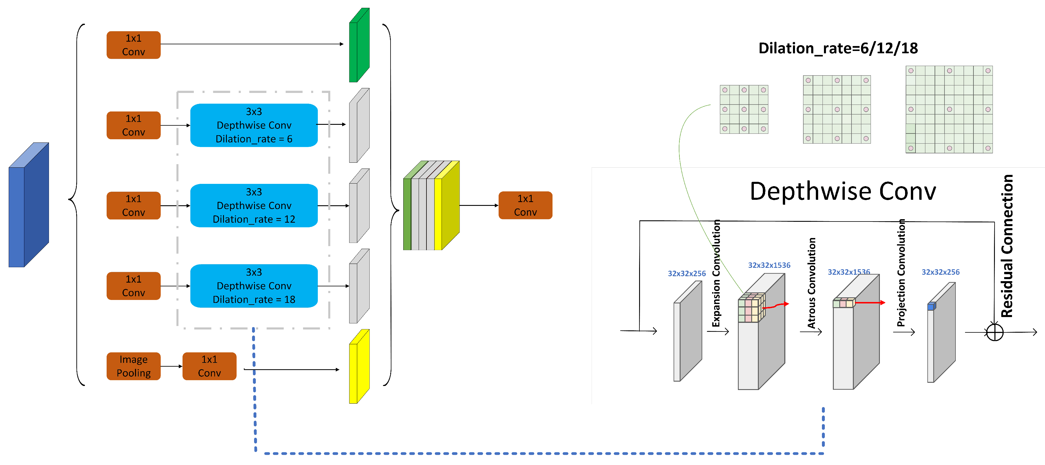
Atrous Bottleneck Pyramid Module (ABPM): The original ASPP module extracts feature maps with different receptive fields by parallel atrous convolutions with various dilation rates. However, its spaced and sparse sampling leads to a lack of correlation between convolution results, causing issues like checkerboard artifacts, feature discontinuities, and spatial gaps. A common solution is to apply upsampling before convolution to avoid these artifacts. Inspired by MobileNetV2’s inverted residual structure, which first expands dimensions, then applies convolution, and finally reduces dimensions while maintaining low computational costs through depthwise separable convolution, this study designs the ABPM. This module extracts features using atrous convolutions in high-dimensional spaces, improving the correlation between extracted features.

(3)

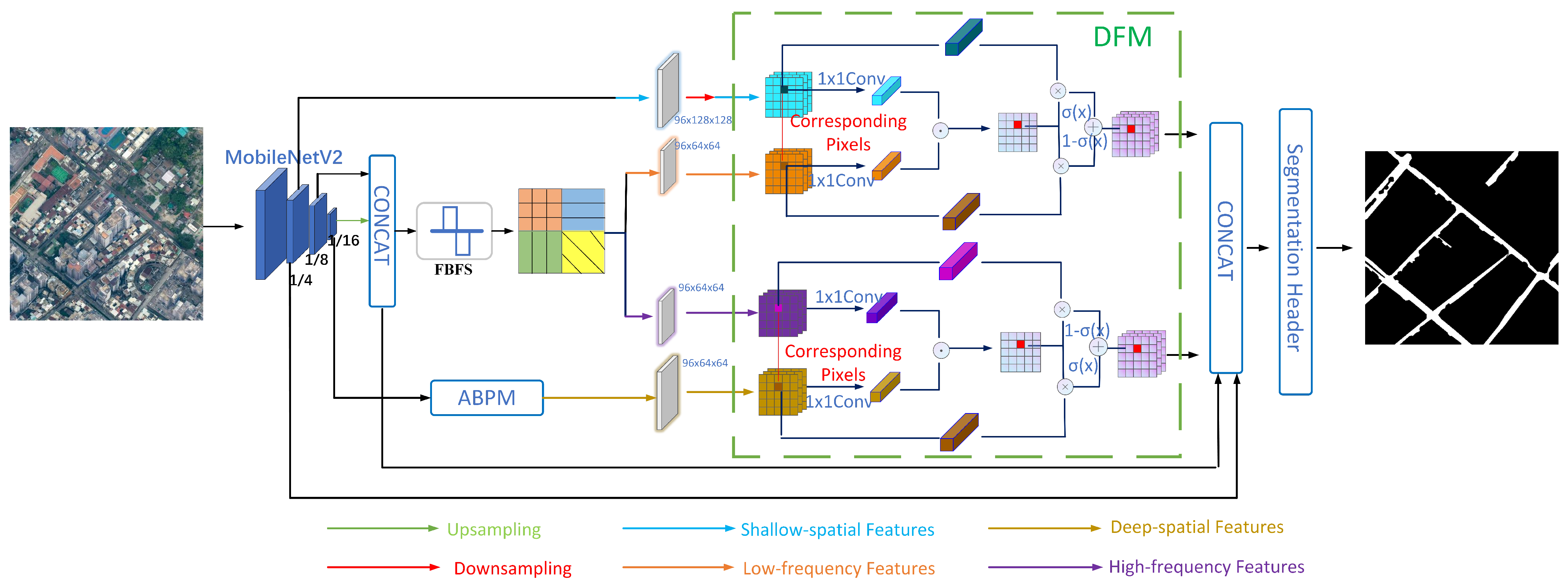
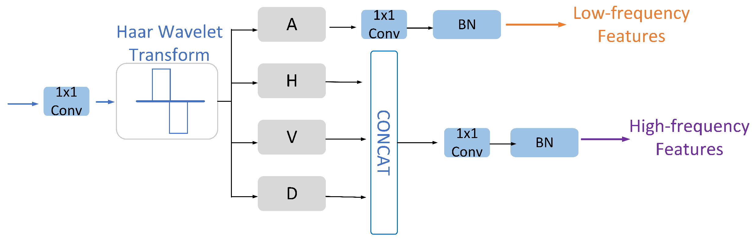
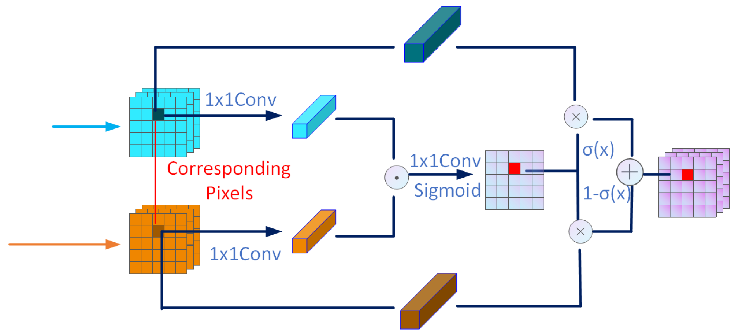
Introducing Frequency Domain Information: A Frequency Band Feature Separator (FBFS) is designed to split the frequency domain features into high-frequency and low-frequency components using Haar wavelet transform. High-frequency features focus on local edges, while low-frequency features emphasize large-area continuous regions and regions. Subsequently, a Domain Fusion Module (DFM) aligns and fuses frequency domain and spatial domain features. High-frequency features are integrated with deep spatial features that carry semantic information, whereas low-frequency features are linked with shallow spatial features that encode positional information. DFM can select features between the frequency domain and spatial domain, effectively bridge the semantic gap between the two features, and make full use of the frequency domain and spatial domain feature information.

2. Materials and Methods

In this section, we first introduce the overall structure of the Cross-Domain Feature Fusion Network (CDFFNet) that has been constructed. Then, we present the three important modules of CDFFNet, namely, Atrous Bottleneck Pyramid Module (ABPM), Frequency Band Feature Separator (FBFS), and Domain Fusion Module (DFM).

2.1. The Overall Structure of CDFFNet

The overall structure of CDFFNet is illustrated in Figure 1. It retains the structure of DeepLabv3+ for thoroughly extracting shallow and deep features in the spatial domain, utilizing the 1/4 low-level feature layer output by the MobileNetV2 backbone network as the shallow feature layer to preserve positional information in the spatial domain. The 1/16 feature map is passed into the Atrous Bottleneck Pyramid Module (ABPM) for multi-scale feature extraction, obtaining deep features that contain spatial domain category information. Subsequently, the output 1/8 and 1/16 feature maps are resized to the same scale and concatenated, then fed into the Frequency Band Feature Separator (FBFS). In FBFS, Haar wavelet transform is utilized to decompose spatial domain features into low-frequency and high-frequency features in the frequency domain. The Domain Fusion Module (DFM) module then selects and combines shallow features, low-frequency features, deep features, and high-frequency features to obtain richer hybrid features. Finally, the hybrid features from the two branches and the feature maps from three scales of the backbone network are concatenated, and the final road extraction result is obtained through the segmentation head.

2.2. Improved Network Module

2.2.1. Atrous Bottleneck Pyramid Module (ABPM)

The original ASPP (Atrous Spatial Pyramid Pooling) module extracts feature map information from different receptive fields by paralleling atrous convolutions with various dilation rates. However, the interval sampling and sparse sampling of atrous convolutions can lead to a lack of correlation between convolution results, causing issues such as the checkerboard effect in image pixels, resulting in discontinuous image features and spatial gaps. A common solution is to perform upsampling before convolution to avoid the generation of artifacts. Inspired by the inverted residual structure in MobileNetV2, which first increases the dimensionality, then applies convolution, and finally reduces the dimensionality, while using depthwise separable convolutions to ensure less computational cost, we design the Atrous Bottleneck Pyramid Module (Figure 2). In this module, atrous convolutions are used for feature extraction in high-dimensional features to increase the correlation between extracted features. Specifically, a 1 × 1 convolution is first used to unify the number of channels in the four branches to 256. Then, three of these branches apply depthwise convolutions with dilation rates set to 6, 12, and 18. Respectively, for feature extraction in high-dimensional features that have been expanded six times. Afterward, pointwise convolutions are used for feature extraction in the channel direction and to restore the channel dimensions. Finally, the features from the four branches and the pooled features are concatenated, and a 1 × 1 convolution is used to change the number of channels:

$$\begin{array}{cc}\hfill {\mathbf{F}}_{\mathbf{ABPM}}& =\sum _{i=1}^3{\delta }_{\mathrm{DS}}^{r_i}\left({\delta }_{1\times 1}\left({\mathbf{F}}_{\mathbf{in}}\right)\right)+{\delta }_{1\times 1}\left({\mathbf{F}}_{\mathbf{in}}\right)+{\delta }_{\mathrm{pool}-\mathrm{conv}}\left({\mathbf{F}}_{\mathbf{in}}\right)\hfill \end{array}$$

(1)

Among them, ${\delta }_{1\times 1}\left(\right)$ represents a 1 × 1 convolution, ${\delta }_{\mathrm{pool}-\mathrm{conv}}\left(\right)$ represents pooling followed by a 1 × 1 convolution, and ${\sum }_{i=1}^3{\delta }_{\mathrm{DS}}^{r_i}\left(\right)$ represents depthwise separable convolutions with dilation rates set to 6, 12, and 18. $r_i$ = 6, 12 and 18. Using ABPM expands the receptive field of the model while preserving important detail information, and at the same time, the parameter count and computational complexity remain largely unchanged due to the use of depthwise separable convolutions with dilation rates.

2.2.2. Frequency Band Feature Separator (FBFS)

To introduce frequency domain information, a Frequency Band Feature Separator (Figure 3) module is designed. This module first employs pointwise convolution to enhance the nonlinearity of features, generating new features with unchanged dimensions. It then utilizes the Haar wavelet transform to decompose frequency domain features into horizontal, vertical, and diagonal high-frequency components, as well as a low-frequency component. The three high-frequency components are concated, and pointwise convolutions and batch normalization are applied separately to obtain high-frequency and low-frequency features embedded in the CNN network. The FBFS module leverages the simplicity and efficiency of the Haar wavelet transform for image signal decomposition to effectively extract frequency domain features, enabling more comprehensive feature representation.

For the input $X\in R^{C\times H\times W}$, a pointwise convolution operation is first performed to enhance feature nonlinearity, resulting in a new feature $X\in R^{C\times H\times W}$ with unchanged dimensions. A first-order Haar wavelet transform is applied to each channel of $X_c\in R^{H\times W}$:

$$\left\{\begin{array}{c}{A}_c(i,j)={\displaystyle \frac{X_c(i,2j-1)+X_c(i,2j)}{2}}\hfill \\ \\ D_c(i,j)=X_c(2i-1,j)-X_c(2i,j)\hfill \end{array}\right.$$

(2)

Here, $A_c(i,j)$ represents the low-frequency approximation coefficients of channel c, $D_c(i,j)$ represents the high-frequency detail coefficients of channel c, where i is the row index and j is the column index. After the first-order Haar wavelet transform, the width of each row is halved, and the range of j changes from 1 to ${\displaystyle \frac{W}{2}}$. Subsequently, the following Haar wavelet transform is applied to each column of the low-frequency approximation coefficients $A_c(i,j)$ and high-frequency detail coefficients $D_c(i,j)$ of channel c:

$$\left\{\begin{array}{c}{A}_c=A{A}_c(i,j)={\displaystyle \frac{A_c(i,2j-1)+A_c(i,2j)}{2}}\hfill \\ H_c=A{D}_c(i,j)={\displaystyle \frac{D_c(i,2j-1)-D_c(i,2j)}{2}}\hfill \\ V_c=D{A}_c(i,j)=A_c(i,2j-1)-A_c(i,2j)\hfill \\ D_c=D{D}_c(i,j)=D_c(i,2j-1)-D_c(i,2j)\hfill \end{array}\right.$$

(3)

Here, $A_c$ represents the approximation coefficients of a single channel, $H_c$ represents the horizontal detail coefficients of a single channel, $V_c$ represents the vertical detail coefficients of a single channel, and $D_c$ represents the diagonal detail coefficients of a single channel. The coefficients $H_c$, $V_c$, and $D_c$ are combined into high-frequency components, while $A_c$ represents the low-frequency component. Both the high-frequency and low-frequency components are subjected to $1\times 1$ convolution for low-dimensional mapping and batch normalization, resulting in high-frequency and low-frequency features:

$$\begin{array}{cc}& F_l,F_h=(\psi \left({\delta }_{1\times 1}\left(A\right)\right),\psi \left({\delta }_{1\times 1}\left(Cat(H,V,D)\right)\right))\hfill \end{array}$$

(4)

Here, ${\delta }_{1\times 1}\left(\right)$ represents the $1\times 1$ convolution, $\psi \left(\right)$ represents batch normalization, and $F_l,F_h\in (C,H/2,W/2)$ represent the low-frequency and high-frequency features, respectively.

2.2.3. Domain Fusion Module (DFM)

Features in the frequency domain and spatial domain capture different aspects and attributes of an image. It is necessary to enhance the information transfer between cross-domain feature maps and selectively fuse spatial and frequency features to improve the model’s representation capability.

Figure 4 illustrates the structure of the Domain Fusion Module (DFM). First, after performing dimensionality reduction using $1\times 1$ convolutions in both the spatial and frequency domains, the corresponding pixel vectors ${\overrightarrow{v}}_s$ and ${\overrightarrow{v}}_f$ are subjected to a dot product operation. The result is then upscaled to the input dimension, and a Sigmoid activation is applied to generate the weight information for the corresponding pixels:

$$\sigma (i,j)=\mathrm{Sig}\left(\mathrm{Upsample}\left({\overrightarrow{v}}_s(i,j)·{\overrightarrow{v}}_f(i,j),C_{\mathrm{in}}\right)\right)$$

(5)

Here, $C_{\mathrm{in}}$ represents the input dimension, Sig() represents the Sigmoid activation function, and $\sigma (i,j)$ denotes the similarity between the corresponding pixels in the spatial and frequency domains. If $\sigma (i,j)$ is high, the spatial domain feature weight becomes larger. The feature selection is performed using $\sigma (i,j)$, and the final fused feature is generated as follows:

$$Ou{t}_{DFM}=\sigma {\overrightarrow{v}}_s+(1-\sigma ){\overrightarrow{v}}_f.$$

(6)

3. Experiments and Analysis

First, the dataset and evaluation metrics used in this experiment will be introduced. Then, the parameters and strategies of the training platform will be presented. Finally, the experimental results of the comparison experiments and ablation experiments, along with their analysis, will be discussed.

3.1. Experimental Settings

3.1.1. Datasets

The CHN6-CUG [37] and Massachusetts [38] datasets are widely used for evaluating road extraction models in remote sensing imagery, ensuring the robustness and generalization ability of the evaluated models. Below is a detailed introduction to these two datasets utilized in this experiment.

CHN6-CUG (50 cm/pixel): This dataset, created by Zhu Qiqi and others from China University of Geosciences (Wuhan), is a large-scale satellite remote sensing road dataset. It contains high-resolution satellite imagery from six representative cities in China, including Beijing and Shanghai. The dataset features pixel-level annotations, categorizing pixels into road and non-road classes with high precision. It comprises a total of 4511 labeled images, each with a resolution of 512 × 512 pixels. Among these, 3608 images are used for model training, while the remaining 903 images are reserved for testing and result evaluation.

Massachusetts (1 m/pixel): This dataset contains a total of 1171 remote sensing images of urban, suburban, and rural scenes. Each image is 1500 × 1500 pixels in size, covering an area of 2.25 km² per image and more than 2600 km² in total. The labeled images are derived from rasterized road centerlines generated using OpenStreetMap vector road data, with a line width of 7 pixels. A random selection of 995 images (85%) is designated as the training set, while 176 images (15%) are used as the test set. To preprocess the data, each 1500 × 1500 image is padded with 18 rows and 18 columns of zero-value pixels on the top, bottom, left, and right sides, converting it to a size of 1536 × 1536 pixels. Subsequently, each image in both the training and test sets is divided into 9 non-overlapping patches of 512 × 512 pixels, resulting in 8955 patches for training and 1584 patches for testing. To reduce training costs, patches containing only zero-value pixels are removed, leaving a final dataset of 8239 training patches and 1355 test patches, along with their corresponding labeled images.

3.1.2. Evaluation Metrics

In this experiment, five commonly used evaluation metrics in remote sensing segmentation are employed to verify the accuracy and inference speed of road extraction for each model. These metrics are as follows: mean Intersection over Union (mIoU), mean Pixel Accuracy (mPA), Recall, Accuracy, the number of parameters (PN) and Frames Per Second (FPS).

mIoU: Intersection over Union (IoU) measures the overlap between the predicted road region and the ground truth road region. The mean Intersection over Union (mIoU) is the average IoU of the road and background classes. The formula is as follows:

$$\mathrm{IoU}={\displaystyle \frac{\mathrm{TP}}{\mathrm{TP}+\mathrm{FP}+\mathrm{FN}}}\mathrm{and}\mathrm{mIoU}={\displaystyle \frac{\sum \mathrm{IoU}}{\mathrm{C}}}$$

(7)

mPA: Pixel Accuracy (PA) represents the proportion of correctly predicted pixels in the road or background category out of the total pixels for that category. The mean Pixel Accuracy (mPA) is the average PA of the road and background classes. The formula is as follows:

$$\mathrm{PA}={\displaystyle \frac{\mathrm{TP}}{\mathrm{TP}+\mathrm{FN}}}\mathrm{and}\mathrm{mPA}={\displaystyle \frac{\sum \mathrm{PA}}{\mathrm{C}}}$$

(8)

Recall: It refers to the proportion of pixels that are correctly predicted by the model among the pixels that are actually road. The formula is as follows:

$$\mathrm{Recall}={\displaystyle \frac{\mathrm{TP}}{\mathrm{TP}+\mathrm{FN}}}$$

(9)

Accuracy: It refers to the proportion of pixels in the image that are correctly predicted by the model as road or background. The formula is as follows:

$$\mathrm{Accuracy}={\displaystyle \frac{\mathrm{TP}}{\mathrm{TP}+\mathrm{FP}+\mathrm{FN}}}$$

(10)

TP (True Positive) refers to the number of pixels correctly predicted as roads, FP (False Positive) refers to the number of pixels incorrectly predicted as roads, FN (False Negative) refers to the number of pixels that are actually roads but predicted as non-roads, TN (True Negative) refers to the number of pixels correctly predicted as non-roads, and C represents the number of classes, which is 2 for road extraction tasks.

Number of Parameters (PN): It represents the sum of all trainable parameters in the model to measure the complexity and computational resource requirements. A lower parameter count enables the model to be deployed on embedded and mobile devices, reducing the energy consumption associated with computation and storage. Additionally, a lower parameter count can help reduce the risk of model overfitting to some extent.

Frames Per Second (FPS): It is used to indicate the number of remote sensing image frames that a model can process or display per second. In real-time application scenarios such as autonomous driving and real-time road extraction, a high FPS means the system can process images or video streams faster, providing more timely road information.

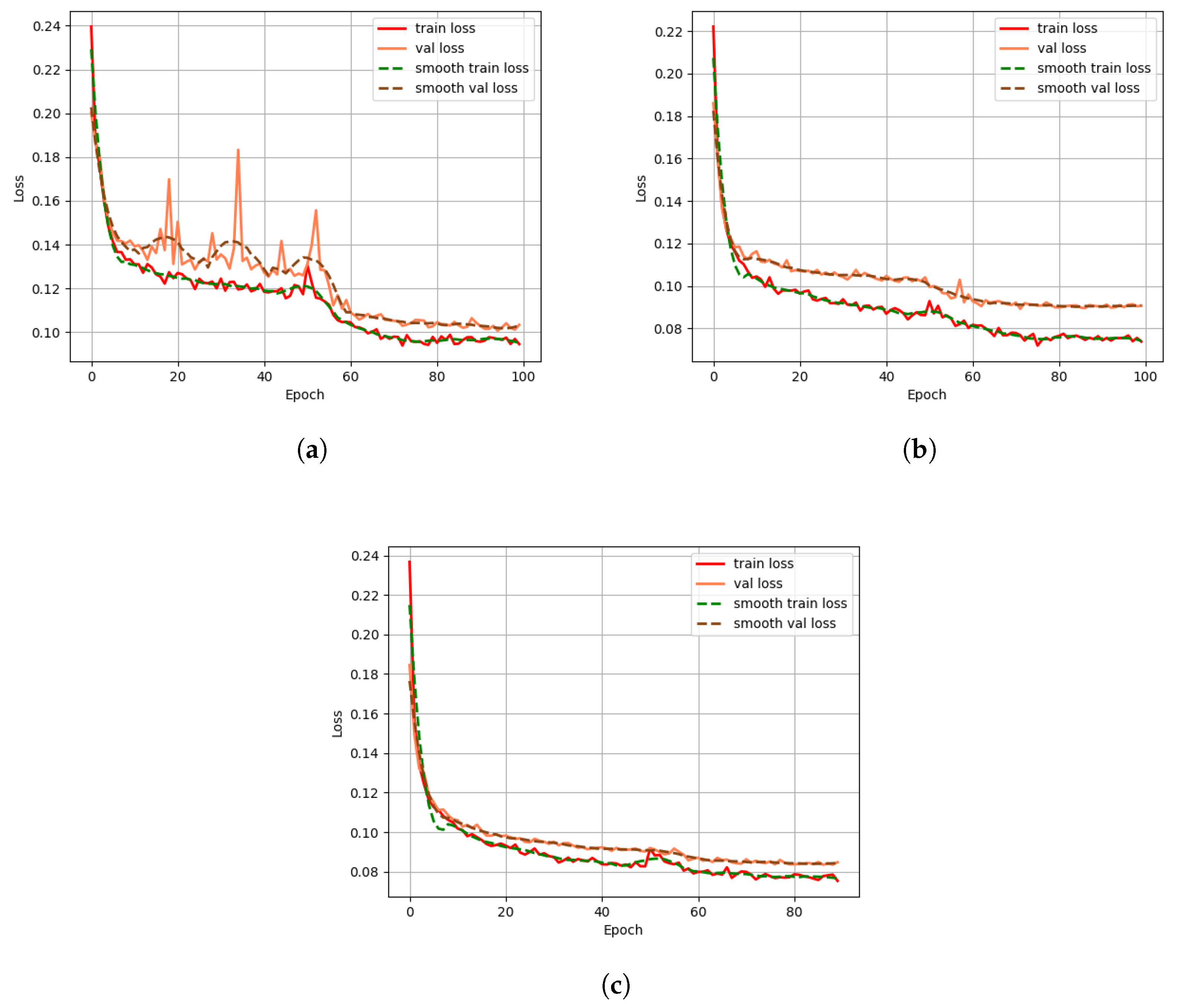
3.1.3. Implementation Details

In this experiment, all road extraction networks use the same hardware setup, loss function, optimizer, learning rate, dataset division, and data augmentation methods.

The hardware setup includes a 13th Gen Intel(R) Core(TM) i5-13500HX CPU running at 2.50 GHz, 16 GB of RAM (Intel Corporation, Santa Clara, CA, USA), and an NVIDIA GeForce RTX 4060 Laptop GPU with 8 GB of VRAM (NVIDIA Corporation, Santa Clara, CA, USA). The algorithm programming environment utilizes PyTorch 1.10.2 with GPU acceleration via CUDA 11.3. The model employs Cross-Entropy (CE) Loss as the loss function, and Stochastic Gradient Descent (SGD) as the optimizer. The learning rate follows a Cosine schedule, starting at a maximum of 7 × 10⁻³ and gradually decreasing to a minimum of 7 × 10⁻⁵. The batch size is set to 8, with a total of 100 epochs for training.

3.2. Comparison with Other Methods

To verify the effectiveness of CDFFNet in remote sensing road extraction, comparative experiments were conducted using the PSPNet [39] model, U-Net model, HRNet [40] model, SegFormer [41] model, RoadCNN [6] model, and the proposed CDFFNet model. The accuracy comparison experiment will compare the differences between the models in the accuracy of road extraction, while the inference efficiency comparison experiment will compare the differences between the models in the number of parameters and the inference speed. Both experiments performed a series of rigorous quantitative and qualitative analyses to better demonstrate their respective strengths and weaknesses in the road extraction task.

To ensure a convenient and fair comparison of performance differences between different road extraction models, all models shared a common training and testing framework. A significant amount of time was invested in debugging the comparative experimental models within the PyTorch 1.10.2. For models originally implemented in Caffe or TensorFlow, where no PyTorch-based source code was available from the original papers, we utilized the implementations of these models found in MMSegmentation (an open-source semantic segmentation framework developed by OpenMMLab), such as PSPNet, UNet, and DeepLabV3+. If a model was not available in MMSegmentation, we searched for its implementation in the source code provided by relevant literature that used the model, for example, RoadCNN, which is sourced from MSMDFF-Net [7]. For models whose original papers directly provided PyTorch framework-based code, we directly used the code for those model architectures, such as HRNet and Segformer.

3.2.1. Accuracy Comparison Experiment

The specific experimental results are shown in

Table 1. Accuracy Metrics on CHN6_CUG. (The bold font indicates the optimal value).

Methods	mIoU/%	mPA/%	Recall/%	Accuracy/%
PSPNet (mobileNetV2)	70.97	77.60	56.63	96.18
U-Net (VGG16)	74.41	81.06	63.41	96.68
HRNet (hrnetv2_w18)	74.58	80.88	62.96	96.74
SegFormer (MixViTb1)	69.63	75.42	52.08	96.09
RoadCNN	73.14	80.78	62.15	96.39
DeepLabv3+ (Xception)	71.08	78.77	59.25	96.05
CDFFNet (MobileNetV2)	74.83	81.86	65.10	96.70

and

Table 2. Metrics on Massachusetts. (The bold font indicates the optimal value).

Methods	mIoU/%	mPA/%	Recall/%	Accuracy/%
PSPNet (mobileNetV2)	52.78	55.02	10.43	96.03
U-Net (VGG16)	68.77	73.13	46.95	97.21
HRNet (hrnetv2_w18)	68.70	74.56	45.98	97.13
SegFormer (MixViTb1)	62.57	66.35	40.32	96.88
Road CNN	68.88	74.17	47.22	97.12
DeepLabv3+ (Xception)	65.94	70.94	42.8	96.82
CDFFNet (MobileNetV2)	69.25	73.8	48.3	97.24

, which, compared to the DeepLabv3+ baseline model, CDFFNet achieves an improvement of 3.75% in mIoU, 3.09% in mPA, 5.85% in Recall, and 0.65% in Accuracy on the CHN6_CUG dataset. On the Massachusetts dataset, CDFFNet achieves an improvement of 3.31% in mIoU, 2.86% in mPA, 5.5% in Recall, and 0.6% in Accuracy, further demonstrating its effectiveness in different remote sensing data contexts. On CHN6_CUG, CDFFNet achieved an mIoU improvement of 3.86%, 0.42%, 0.25%, 5.2%, and 1.69% compared to the PSPNet, U-Net, HRNet, SegFormer, and RoadCNN models, respectively. The mPA metric increased by 4.1%, 0.8%, 0.98%, 6.44%, and 1.08%, while the Recall metric showed an increase of 8.47%, 1.69%, 2.41%, 13.02%, and 2.95%, respectively. The accuracy values are quite close, but CDFFNet achieves the highest value. Additionally, CDFFNet demonstrated superior accuracy on the Massachusetts dataset, reflecting its generalization capability. Among them, HRNet performs well, showing little difference in accuracy metrics compared to CDFFNet. However, the CDFFNet model processes remote sensing images of 512 × 512 resolution at approximately three times the speed of HRNet. Specific details are provided in Section 3.2.2, Inference Efficiency Comparison Experiment.

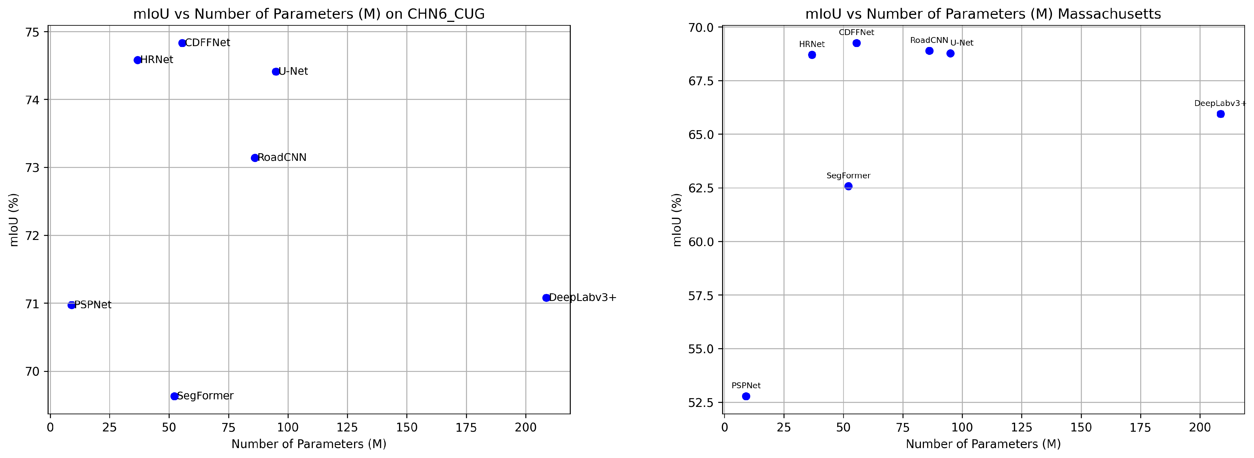
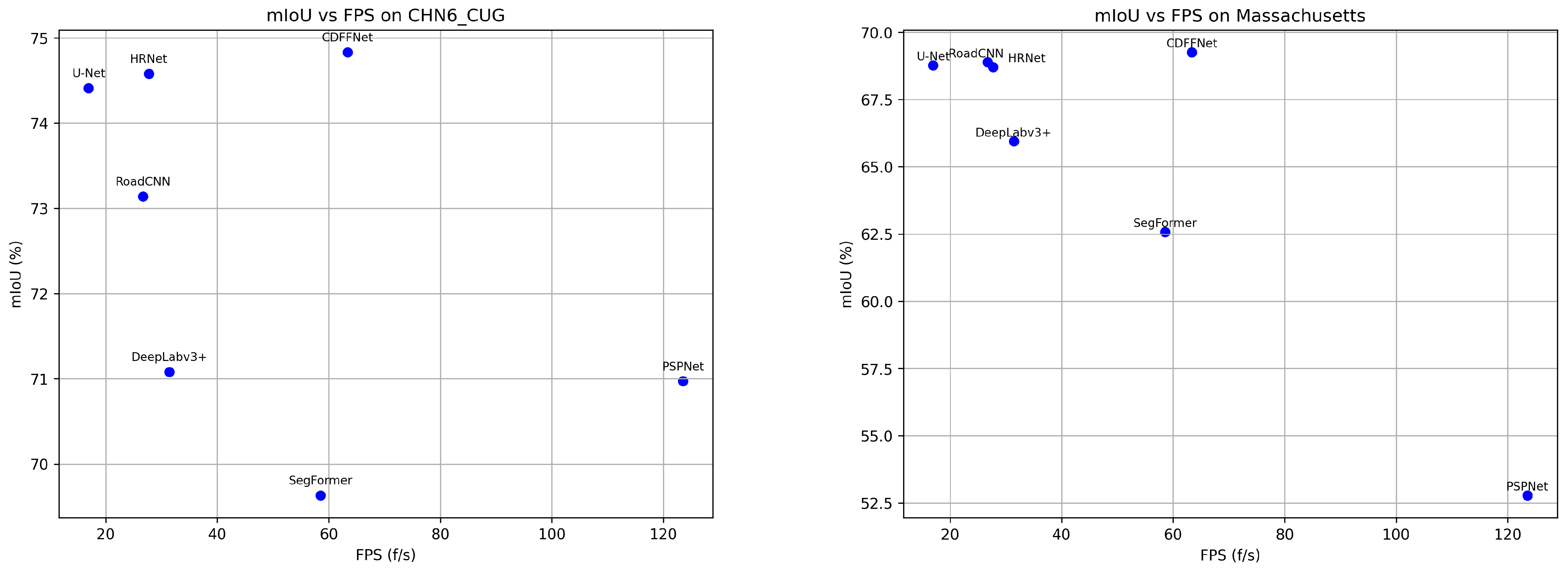
3.2.2. Inference Efficiency Comparison Experiment

Table 3. PN and FPS Metrics of Each Model.

Methods	PSPNet	U-Net	HRNet	SegFormer	RoadCNN	v3+	CDFFNet
PN/M	9.06	94.95	36.76	52.18	86.15	208.70	55.57
FPS (f/s)	123.54	16.95	27.74	58.55	26.69	31.41	63.36

summarizes the number of parameters (PN) and Frames Per Second (FPS) of each model on 512 × 512 resolution remote sensing images. The FPS for each model were obtained by performing multiple measurements under the same hardware conditions and averaging the results. From the table, it can be observed that after lightweight improvements to the DeepLabV3+ baseline model, the number of parameters was reduced by 153.13 M, while the prediction speed increased by 31.95 f/s. The PSPNet with MobileNetV2 as the backbone has 46.51 M fewer parameters than CDFFNet, and its inference speed increased by 60.18 f/s. However, CDFFNet outperforms PSPNet in terms of road extraction accuracy. Although HRNet and SegFormer have fewer parameters, HRNet’s processing of high-resolution images and the use of the Transformer encoder in SegFormer reduce their inference speeds.

The following four scatter plots show the relative relationship between the Number of Parameters, FPS, and mIoU for each model on the CHN6_CUG and Massachusetts datasets.

As shown in Figure 5, on the CHN6_CUG dataset, DeepLabv3+ (208.7 M parameters), and RoadCNN (86.15 M parameters) models, which have a larger number of parameters, perform poorly, with mIoU values 3.57% and 1.69% lower than CDFFNet, respectively. This is because larger models tend to capture detailed information, including noise and outliers, during training on smaller datasets. When the dataset is smaller, the model can memorize the details of the training set but fails to generalize to the validation set. On the larger Massachusetts dataset, RoadCNN, with more parameters, can fully exploit its performance, with the mIoU only differing by 0.37% from CDFFNet. U-Net and HRNet, which have moderate parameter counts, maintain relatively low computational overhead while achieving high performance, with mIoU values differing from CDFFNet by only 0.42% and 0.25%, respectively. However, as analyzed in Figure 6, U-Net and HRNet have lower FPS performance. U-Net employs a multi-layer encoder–decoder structure and incorporates skip connections, gradually reducing the spatial resolution and increasing feature channels in the encoder while using skip connections to combine encoder features and gradually restoring spatial resolution in the decoder. HRNet processes high-resolution and low-resolution feature maps through multiple parallel branches and fuses pixel-wise information at different scales to obtain rich semantic information. The special structure of U-Net and HRNet significantly reduces the inference efficiency and image prediction speed, affecting the application of road extraction in real-time scenarios. PSPNet has the least parameters and the highest inference speed, but its road extraction accuracy is far behind that of CDFFNet. In summary, CDFFNet strikes an excellent balance between road extraction accuracy, model complexity, and inference speed, providing an effective reference for the real-time extraction of road information in engineering applications.

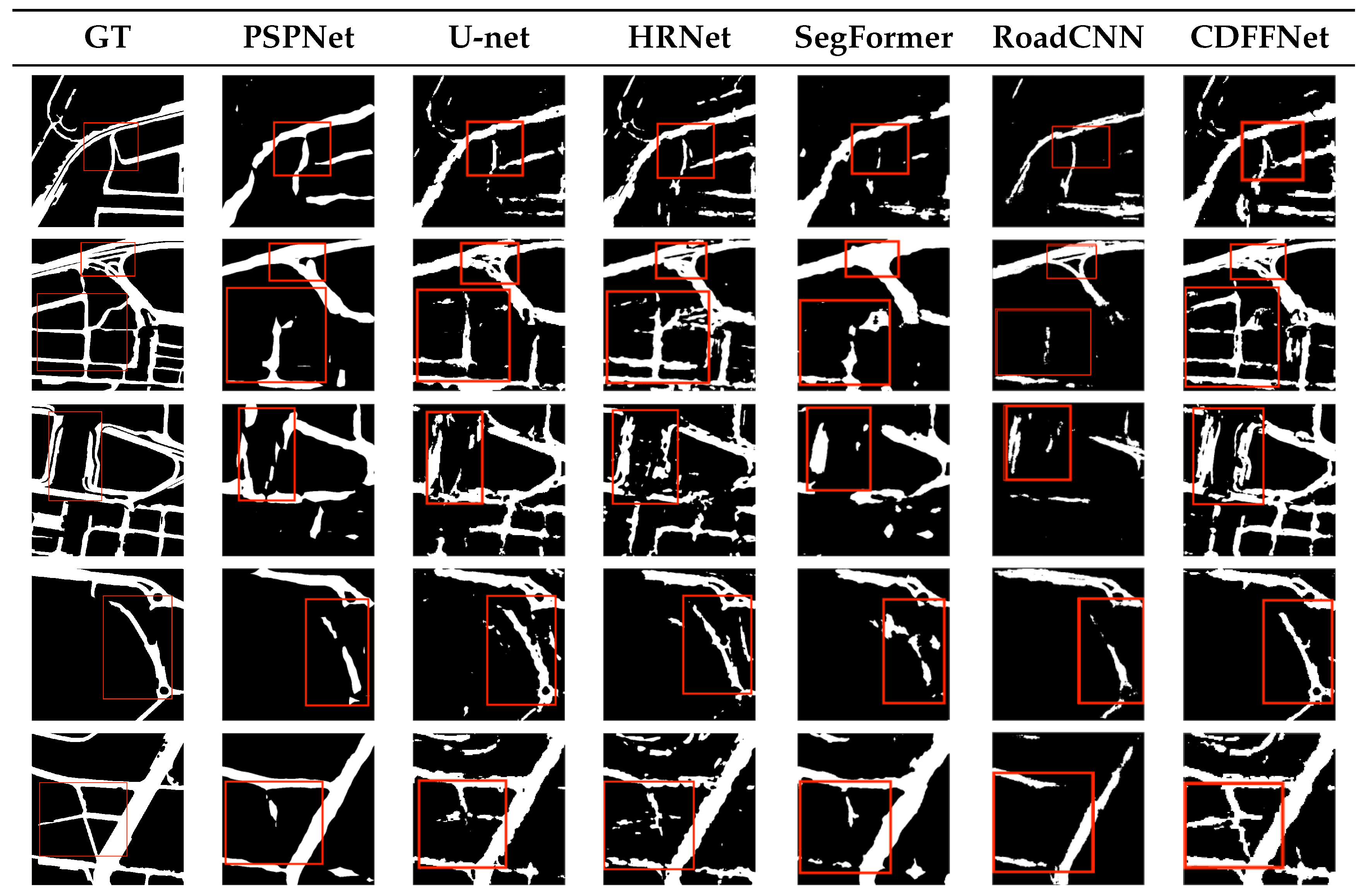
3.2.3. Comparison Experiment Prediction Results

The comparison of prediction results for different models is shown in Figure 7. In order to more clearly differentiate the road segmentation results generated by the models, the road areas in the prediction results are marked in white, and the non-road areas in black. Furthermore, to highlight the differences in key regions, red bounding boxes are used for marking. The reference models exhibit varying degrees of misclassification, omission, and discontinuous segmentation in the road extraction task. In contrast, the CDFFNet model achieves more accurate identification of road targets at different scales, effectively capturing road edge information, and delivering significantly better prediction results compared to other models.

3.3. Ablation Experiments

To further evaluate the contribution of each improved part, ablation experiments were conducted using the CHN6_CUG dataset, gradually incorporating the improvements into the baseline model DeepLabV3+.

Table 4. Ablation Experiment Results.

Method	mIoU/%	mPA/%	Recall%	Accuracy/%	PN/M
DeepLabV3+	71.08	78.77	59.25	96.05	208.70
+MobileNetV2	72.74	79.21	59.74	96.46	22.18
+ABPM	73.65	80.81	63.08	96.52	31.76
+FBFS	74.58	81.56	64.83	96.65	55.64
+DFM	74.83	81.86	65.10	96.70	55.57

presents the experimental results of the baseline model after replacing the backbone network (MobileNetV2), adding the ABPM, FBFS and DFM. In the ablation experiment for the FBFS module, the shallow and deep features from the spatial domain, as well as the high- and low-frequency features from the frequency domain, were concatenated along the channel dimension separately. These concatenated features were then passed through a 1 × 1 convolution to adjust the channel dimensions before being fed into the Segmentation Header.

From the analysis of the ablation experiments, it can be concluded that using MobileNetV2 as the backbone network significantly reduces the number of parameters while improving the segmentation accuracy of the model. Replacing ASPP with the ABPM module increases the parameter count due to the use of high-dimensional features and residual connections, but the precision of road extraction improved significantly. Finally, introducing frequency-domain features further enhances the model’s ability to extract roads in shaded areas. Figure 6 shows the improvement in the model’s extraction results for roads in shadowed areas after adding frequency domain information.

The loss changes during the training and validation process for the original DeepLabV3+, the model with the MobileNetV2 backbone, and the final CDFFNet are shown in Figure 8. DeepLabV3+ has a larger number of parameters, requiring more training steps to effectively learn the patterns in the data, resulting in a slower convergence of the loss value. Additionally, larger models often have more local minima and saddle points, making the optimization process more challenging, causing the loss value to fluctuate continuously. After replacing the backbone with MobileNetV2, the model structure was lightweighted, and the loss value decreased consistently in the early stages of training. The fluctuation of the loss value was significantly reduced, and the optimization process became more stable. The training and validation loss of CDFFNet showed a more stable decline, with the final validation loss also decreasing after model improvement, demonstrating CDFFNet’s better generalization ability in road extraction tasks.

From the analysis of the ablation experiments, it can be concluded that using MobileNetV2 as the backbone network significantly reduced the number of parameters while improving the segmentation accuracy of the model. Replacing ASPP with the ABPM module increased the parameter count due to the use of high-dimensional features and residual connections, but the precision of road extraction improved significantly. Finally, introducing frequency-domain features further enhanced the model’s ability to extract roads in shaded areas. Figure 9 shows the improvement in the model’s extraction results for roads in shadowed areas after adding frequency domain information.

4. Conclusions

This paper proposes a lightweight Cross-Domain Feature Fusion Network (CDFFNet) to address the negative impact of areas with significant grayscale variations, such as tree shadows and road edges, on road extraction results in remote sensing image tasks. The network introduces a frequency-domain information auxiliary branch into the spatial-domain road extraction model to fully integrate spatial and frequency-domain features, improving the accuracy and connectivity of road extraction. First, a lightweight backbone network, MobileNetV2, is used to replace Xception in the DeepLabV3+ framework, reducing the model’s parameter count, lowering computational complexity, and maintaining efficient feature extraction capabilities. The Atrous Bottleneck Pyramid Module (ABPM) is used for multi-scale feature extraction to learn deep spatial domain features. The Frequency Band Feature Separator (FBFS) performs frequency-domain feature mapping (low-frequency and high-frequency) using Haar wavelet transform to obtain additional frequency-domain information. Then, through the Domain Fusion Module (DFM) module, the information transfer between cross-domain feature maps is enhanced, and spatial–frequency features are selectively fused. The final experimental results validate the superiority of the CDFFNet architecture and the effectiveness of each improvement.

Compared to traditional models, CDFFNet not only achieves significant improvements in accuracy but also effectively reduces memory requirements and substantially boosts inference speed. By striking a good balance among parameter count, accuracy, and inference speed, CDFFNet offers crucial advantages and flexibility for the practical deployment of road extraction models. This optimization enables CDFFNet to operate efficiently on resource-constrained edge devices, reducing hardware costs and power consumption while maintaining high-precision road extraction capabilities. Therefore, CDFFNet is particularly suitable for tasks requiring efficient and accurate road extraction, such as urban planning, disaster management, and traffic monitoring. In the future, we will improve CDFFNet for different edge devices to enhance its application value.

References

1. Hou, Z.Q.; Chen, Y.; Yuan, W.H.; Chen, J.M. The Study on the Recent Suspended Sediment Variation Characteristics in Yangshan Deepwater Port Area Based on Landsat 8 Satellite Data. Port Waterw. Eng. 2024, 27–33+40. [Google Scholar] [CrossRef]
2. Yang, A.Q.; Yu, X.H.; Chen, L.; Yan, S.M.; Zhu, L.Y.; Guo, W.; Li, M.M.; Li, Y.Y.; Li, Y.; He, J.Y. Long-term Trend of HCHO Column Concentration in Shanxi Based on Satellite Remote Sensing. China Environ. Sci. 2024, 44, 6608–6616. [Google Scholar] [CrossRef]
3. Xu, Q.; Long, C.; Yu, L.; Zhang, C. Road extraction with satellite images and partial road maps. IEEE Trans. Geosci. Remote Sens. 2023, 61, 4501214. [Google Scholar] [CrossRef]
4. Zhang, Y.; Zhang, J.; Li, T.; Sun, K. Road Extraction and Intersection Detection Based on Tensor Voting. In Proceedings of the 2016 IEEE International Geoscience and Remote Sensing Symposium (IGARSS), Beijing, China, 10–15 July 2016; pp. 1587–1590. [Google Scholar]
5. Huang, B.; Zhao, B.; Song, Y. Urban land-use mapping using a deep convolutional neural network with high spatial resolution multispectral remote sensing imagery. Remote Sens. Environ. 2018, 214, 73–86. [Google Scholar] [CrossRef]
6. Bastani, F.; He, S.; Abbar, S.; Alizadeh, M.; Balakrishnan, H.; Chawla, S.; Madden, S.; DeWitt, D. Roadtracer: Automatic Extraction of Road Networks from Aerial Images. In Proceedings of the IEEE Conference on Computer Vision and Pattern Recognition, Salt Lake City, UT, USA, 18–23 June 2018; pp. 4720–4728. [Google Scholar]
7. Wang, Y.; Tong, L.; Luo, S.; Xiao, F.; Yang, J. A Multi-Scale and Multi-Direction Feature Fusion Network for Road Detection From Satellite Imagery. IEEE Trans. Geosci. Remote Sens. 2024, 62, 5615718. [Google Scholar]
8. Chen, H.; Li, Z.; Wu, J.; Xiong, W.; Du, C. SemiRoadExNet: A semi-supervised network for road extraction from remote sensing imagery via adversarial learning. ISPRS J. Photogramm. Remote Sens. 2023, 198, 169–183. [Google Scholar] [CrossRef]
9. Bose, S.; Chowdhury, R.S.; Pal, D.; Bose, S.; Banerjee, B.; Chaudhuri, S. Multiscale probability map guided index pooling with attention-based learning for road and building segmentation. ISPRS J. Photogramm. Remote Sens. 2023, 206, 132–148. [Google Scholar] [CrossRef]
10. Zhang, L.; Lan, M.; Zhang, J.; Tao, D. Stagewise unsupervised domain adaptation with adversarial self-training for road segmentation of remote-sensing images. IEEE Trans. Geosci. Remote Sens. 2021, 60, 5609413. [Google Scholar] [CrossRef]
11. Ding, L.; Bruzzone, L. DiResNet: Direction-aware residual network for road extraction in VHR remote sensing images. IEEE Trans. Geosci. Remote Sens. 2020, 59, 10243–10254. [Google Scholar] [CrossRef]
12. Sun, W.; Wang, R. Fully convolutional networks for semantic segmentation of very high resolution remotely sensed images combined with DSM. IEEE Geosci. Remote Sens. Lett. 2018, 15, 474–478. [Google Scholar] [CrossRef]
13. Weng, W.; Zhu, X. UNet: Convolutional networks for biomedical image segmentation. IEEE Access 2021, 9, 16591–16603. [Google Scholar] [CrossRef]
14. Chen, L.C. Semantic image segmentation with deep convolutional nets and fully connected CRFs. arXiv 2014, arXiv:1412.7062. [Google Scholar]
15. Chen, L.C.; Papandreou, G.; Kokkinos, I.; Murphy, K.; Yuille, A.L. Deeplab: Semantic image segmentation with deep convolutional nets, atrous convolution, and fully connected crfs. IEEE Trans. Pattern Anal. Mach. Intell. 2017, 40, 834–848. [Google Scholar] [CrossRef] [PubMed]
16. Chen, L.C. Rethinking atrous convolution for semantic image segmentation. arXiv 2017, arXiv:1706.05587. [Google Scholar]
17. Chen, L.C.; Zhu, Y.; Papandreou, G.; Schroff, F.; Adam, H. Encoder-Decoder with Atrous Separable Convolution for Semantic Image Segmentation. In Proceedings of the European Conference on Computer Vision (ECCV), Munich, Germany, 8–14 September 2018; pp. 801–818. [Google Scholar]
18. Chaurasia, A.; Culurciello, E. Linknet: Exploiting Encoder Representations for Efficient Semantic Segmentation. In Proceedings of the 2017 IEEE visual communications and image processing (VCIP), St. Petersburg, FL, USA, 10–13 December 2017; pp. 1–4. [Google Scholar]
19. Zhou, L.; Zhang, C.; Wu, M. D-LinkNet: LinkNet with Pretrained Encoder and Dilated Convolution for High Resolution Satellite Imagery Road Extraction. In Proceedings of the IEEE Conference on Computer Vision and Pattern Recognition Workshops, Salt Lake City, UT, USA, 18–23 June 2018; pp. 182–186. [Google Scholar]
20. Mei, J.; Li, R.J.; Gao, W.; Cheng, M.M. CoANet: Connectivity attention network for road extraction from satellite imagery. IEEE Trans. Image Process. 2021, 30, 8540–8552. [Google Scholar] [CrossRef]
21. Qi, Y.; He, Y.; Qi, X.; Zhang, Y.; Yang, G. Dynamic Snake Convolution Based on Topological Geometric Constraints for Tubular Structure Segmentation. In Proceedings of the IEEE/CVF International Conference on Computer Vision, Paris, France, 2–3 October 2023; pp. 6070–6079. [Google Scholar]
22. Oner, D.; Koziński, M.; Citraro, L.; Dadap, N.C.; Konings, A.G.; Fua, P. Promoting connectivity of network-like structures by enforcing region separation. IEEE Trans. Pattern Anal. Mach. Intell. 2021, 44, 5401–5413. [Google Scholar] [CrossRef]
23. Yang, Z.; Zhou, D.; Yang, Y.; Zhang, J.; Chen, Z. Road extraction from satellite imagery by road context and full-stage feature. IEEE Geosci. Remote Sens. Lett. 2022, 20, 8000405. [Google Scholar] [CrossRef]
24. Zhang, Z.; Liu, Q.; Wang, Y. Road extraction by deep residual u-net. IEEE Geosci. Remote Sens. Lett. 2018, 15, 749–753. [Google Scholar] [CrossRef]
25. He, K.; Zhang, X.; Ren, S.; Sun, J. Deep Residual Learning for Image Recognition. In Proceedings of the IEEE Conference on Computer Vision and Pattern Recognition, Las Vegas, NV, USA, 27–30 June 2016; pp. 770–778. [Google Scholar]
26. Yang, X.; Li, X.; Ye, Y.; Lau, R.Y.; Zhang, X.; Huang, X. Road detection and centerline extraction via deep recurrent convolutional neural network U-Net. IEEE Trans. Geosci. Remote Sens. 2019, 57, 7209–7220. [Google Scholar] [CrossRef]
27. Zhipeng, S.; Jingwen, L.; Jianwu, J.; Yanling, L.; Ming, Z. Remote Sensing Image Semantic Segmentation Method Based on Improved DeepLabV3+. Laser Optoelectron. Prog. 2023, 60, 0628003. [Google Scholar]
28. Wulamu, A.; Shi, Z.; Zhang, D.; He, Z. Multiscale road extraction in remote sensing images. Comput. Intell. Neurosci. 2019, 2019, 2373798. [Google Scholar] [CrossRef] [PubMed]
29. Wang, R.; Cai, M.; Xia, Z. A lightweight high-resolution RS image road extraction method combining multi-scale and attention mechanism. IEEE Access 2023, 11, 108956–108966. [Google Scholar] [CrossRef]
30. Bandara, W.G.C.; Valanarasu, J.M.J.; Patel, V.M. Spin Road Mapper: Extracting Roads from Aerial Images via Spatial and Interaction Space Graph Reasoning for Autonomous Driving. In Proceedings of the 2022 International Conference on Robotics and Automation (ICRA), Philadelphia, PA, USA, 23–27 May 2022; pp. 343–350. [Google Scholar]
31. Gao, F.; Wang, X.; Gao, Y.; Dong, J.; Wang, S. Sea ice change detection in SAR images based on convolutional-wavelet neural networks. IEEE Geosci. Remote Sens. Lett. 2019, 16, 1240–1244. [Google Scholar] [CrossRef]
32. Zhao, C.; Xia, B.; Chen, W.; Guo, L.; Du, J.; Wang, T.; Lei, B. Multi-scale wavelet network algorithm for pediatric echocardiographic segmentation via hierarchical feature guided fusion. Appl. Soft Comput. 2021, 107, 107386. [Google Scholar] [CrossRef]
33. Xu, C.; Jia, W.; Wang, R.; Luo, X.; He, X. Morphtext: Deep morphology regularized accurate arbitrary-shape scene text detection. IEEE Trans. Multimed. 2022, 25, 4199–4212. [Google Scholar] [CrossRef]
34. Xu, C.; Fu, H.; Ma, L.; Jia, W.; Zhang, C.; Xia, F.; Ai, X.; Li, B.; Zhang, W. Seeing Text in the Dark: Algorithm and Benchmark. In Proceedings of the 32nd ACM International Conference on Multimedia, Melbourne, Australia, 28 October–1 November 2024; pp. 2870–2878. [Google Scholar]
35. Sandler, M.; Howard, A.; Zhu, M.; Zhmoginov, A.; Chen, L.C. Mobilenetv2: Inverted Residuals and Linear Bottlenecks. In Proceedings of the IEEE Conference on Computer Vision and Pattern Recognition, Salt Lake City, UT, USA, 18–23 June 2018; pp. 4510–4520. [Google Scholar]
36. Chollet, F. Xception: Deep Learning with Depthwise Separable Convolutions. In Proceedings of the IEEE Conference on Computer Vision and Pattern Recognition, Honolulu, HI, USA, 21–26 July 2017; pp. 1251–1258. [Google Scholar]
37. Ross, T.Y.; Dollár, G. Focal Loss for Dense Object Detection. In Proceedings of the IEEE Conference on Computer Vision and Pattern Recognition, Honolulu, HI, USA, 21–26 July 2017; pp. 2980–2988. [Google Scholar]
38. Mnih, V. Machine Learning for Aerial Image Labeling. Ph.D. Thesis, University of Toronto, Toronto, ON, Canada, 2013. [Google Scholar]
39. Zhao, H.; Shi, J.; Qi, X.; Wang, X.; Jia, J. Pyramid Scene Parsing Network. In Proceedings of the IEEE Conference on Computer Vision and Pattern Recognition, Honolulu, HI, USA, 21–26 July 2017; pp. 2881–2890. [Google Scholar]
40. Sun, K.; Zhao, Y.; Jiang, B.; Cheng, T.; Xiao, B.; Liu, D.; Mu, Y.; Wang, X.; Liu, W.; Wang, J. High-resolution representations for labeling pixels and regions. arXiv 2019, arXiv:1904.04514. [Google Scholar]
41. Xie, E.; Wang, W.; Yu, Z.; Anandkumar, A.; Alvarez, J.M.; Luo, P. SegFormer: Simple and efficient design for semantic segmentation with transformers. Adv. Neural Inf. Process. Syst. 2021, 34, 12077–12090. [Google Scholar]
Figure 1. Cross-Domain Feature Fusion Network (CDFFNet).
Applsci 15 01968 g001
Figure 2. Atrous Bottleneck Pyramid Module (ABPM).
Applsci 15 01968 g002
Figure 3. Frequency Band Feature Separator.
Applsci 15 01968 g003
Figure 4. Domain Fusion Module.
Applsci 15 01968 g004
Figure 5. Parameters (M) vs. mIoU.
Applsci 15 01968 g005
Figure 6. FPS vs. mIoU.
Applsci 15 01968 g006
Figure 7. Segmentation results of different methods. GT, Ground Truth.
Applsci 15 01968 g007
Figure 8. Training and validation loss variations: (a) DeepLabV3+. (b) After replacing the backbone network with MobileNetV2. (c) CDFFNet.
Applsci 15 01968 g008
Figure 9. The prediction results for roads in shadowed areas. RS, Remote Sensing; GT, Ground Truth. Before: The Prediction results before adding frequency domain features. After: The Prediction results after adding frequency domain features.
Applsci 15 01968 g009