Article

Dam Deformation Monitoring Model Based on Deep Learning and Split Conformal Quantile Prediction

Department of Water Resources and Harbor Engineering, Fuzhou University, Fuzhou 350100, China
*
Author to whom correspondence should be addressed.
Appl. Sci. 2025, 15(4), 1960; https://doi.org/10.3390/app15041960
Submission received: 20 December 2024 / Revised: 22 January 2025 / Accepted: 11 February 2025 / Published: 13 February 2025

Abstract

:
The construction of an interval prediction model capable of explaining deformation uncertainties is crucial for the long-term safe operation of dams. High effective coverage and narrow interval coverage widths are two key benchmarks to ensure that the prediction interval (PI) can accurately quantify deformation uncertainties. The vast majority of existing models neglect to control the interval coverage width, and overly wide PIs can cause decision confusion when operators are developing safety plans for hydraulic structures. To address this problem, this paper proposes a novel interval prediction model combining bidirectional long-short-term memory network (Bi-LSTM) and split conformal quantile prediction (SCQP) for dam deformation prediction. The model uses Bi-LSTM as a benchmark regressor to extract and explain the nonlinear feature of dam deformation in the continuous time domain. SCQP is used to quantify the uncertainties in dam deformation prediction to ensure that the constructed PI can achieve high effective coverage while further improving the accuracy of the quantification of deformation uncertainties. The effectiveness of the proposed model is validated using deformation monitoring data collected from an arch dam in China. The results show that the average prediction interval effective coverage (PICP) of the proposed model is as high as 0.951 while the mean prediction interval width (MPIW) and coverage width-based criterion (CWC) are both only 5.815 mm. Compared with other models, the proposed method can construct higher-quality PIs, thus providing a better service for the safety assessment of dams.

1. Introduction

Dams, playing an irreplaceable role in providing energy, maintaining ecology, and resisting flooding, are one of the main hydraulic structures that guarantee the socioeconomic prosperity of many countries [1,2]. While dams bring tremendous social benefits, their potential risk cannot be ignored. The cracking or failure of a dam can cause serious damage to people’s lives and ecosystems in the surrounding areas. Therefore, in order to ensure the long-term safe operation of dams, it is very important to carry out long-term safety monitoring of their condition indicators [3]. Among various monitoring targets, deformation is the most intuitive reflection of the safety status of the dam structure [4,5]. Long-term monitoring and predictive modeling of deformation can help operators identify potential risks of dams, which can prevent crack deterioration and failure [6,7].
With the rapid development of computer technology, researchers are increasingly interested in artificial intelligence (AI) applications [8,9]. Therefore, dam deformation prediction using machine learning (ML) and deep learning (DL) regression algorithms is also a hot topic. Simple execution, efficient computation, and high accuracy are advantages of dam deformation prediction models constructed based on AI algorithms [10,11,12,13]. Dai et al. (2018) developed a dam displacement prediction model using a random forest algorithm [14]. This approach can quantify the importance of explanatory variables, subsequently reducing the impact of dimensional catastrophes on the model’s predictive accuracy. Kang et al. (2017) used ELM to explain the structural behavior of concrete dams, and its generalization and computational efficiency have been verified in real engineering projects [15]. Ren et al. (2021) proposed a long- and short-term memory neural network (LSTM) incorporating a mixed attention mechanism and used it for dam displacement prediction [16]. This model not only utilizes DL techniques to break through the limitations of ML models and statistical models due to static regression but also uses the mixed attention mechanism to further enhance the physical interpretability of data-driven models. Song et al. (2023) proposed a novel DL network called SSA-Bi-LSTM for dam safety assessment considering extreme loading conditions [17]. The results showed that the model constructed based on a bidirectional long-short-term memory network (Bi-LSTM) has great generalization potential in dam safety assessment and is better than standard LSTM. Compared with conventional unidirectional DL neural networks, the additional backward LSTM layer introduced by Bi-LSTM allows it to consider the future samples when interpreting time-series lags between sequences [18]. Furthermore, the double-layer LSTM increases the memory threshold, enhancing the model’s depth and breadth for data mining [18,19]. Inspired by the study, we use it as one of the main methods in this work to further explore the potential of Bi-LSTM for dam deformation prediction.
However, there are significant uncertainties in the prediction modeling of dam deformation. According to Refs. [20,21,22], these uncertainties are mainly related to the deformation randomness triggered by the synergistic effect of internal and external factors of the dam, the strong perturbation noise in the data recording process, and the mapping randomness of AI technology [20]. Figure 1 shows the effect of uncertainties in dam deformation prediction. From Figure 1, it can be found that ignoring the deformation uncertainties may greatly affect the credibility of the dam deformation model.
Interval prediction is a tool that can quantify uncertainty by constructing a prediction interval (PI) [23]. Currently, the effectiveness of the methods has now been initially validated in dam deformation prediction. For example, Li et al. (2021) proposed a hybrid approach for concrete dam displacement prediction under uncertain conditions, which integrates principal component analysis (PCA), fuzzy C-means (FCM), and gaussian process regression (GPR) [22]. This approach can generate both PIs and accurate point predictions for dam deformation. Ren et al. (2022) used the improved gradient quantile regression (QR) for dam displacement interval prediction and obtained good results [21]. Yang et al. (2022) combined eXtreme gradient boosting (XGBOOST) with an artificial neural network (ANN) to construct a dam deformation interval prediction model [24]. The model can quantify the uncertainties of dam deformation by multiple random unrepeated sampling of samples. Although the interval prediction models developed in these studies have obtained good results in engineering cases, various stringent data distribution requirements limit their practical value [25]. More importantly, these models may trigger confusion in safety decisions due to the lack of control over the interval coverage width.
Under the influence of complex environmental factors, deformation uncertainties tend to show strong non-homogeneous characteristics. The coverage width of the PIs constructed by the majority of models is relatively fixed, which cannot reflect the evolution process of deformation uncertainties [26]. In addition, these models typically produce too large interval coverage width to satisfy the prediction interval nominal confidence (PINC), which can lead to decision-makers not being able to assess accurately the level of deformation uncertainty [27]. In fact, the ideal high-quality PIs should have the properties of both high effective coverage and narrow interval coverage width [28].
In order to solve these problems, this paper develops a dam deformation interval prediction model that integrates split conformal quantile prediction (SCQP) and Bi-LSTM. The proposed model is capable of constructing high-quality deformation PIs, providing a reliable scientific basis for the safe operation of dams. Its effectiveness and superiority have been demonstrated in an arch dam. The main contributions and innovations of this work can be summarized as follows:
(1)
The Bi-LSTM is used to capture the nonlinear properties of dam deformation, which ensures the generalization ability and robustness of our proposed model.
(2)
Split conformal quantile prediction (SCQP) is applied to quantify the uncertainties of dam deformation prediction, enabling the model to construct high-quality deformation PIs.
(3)
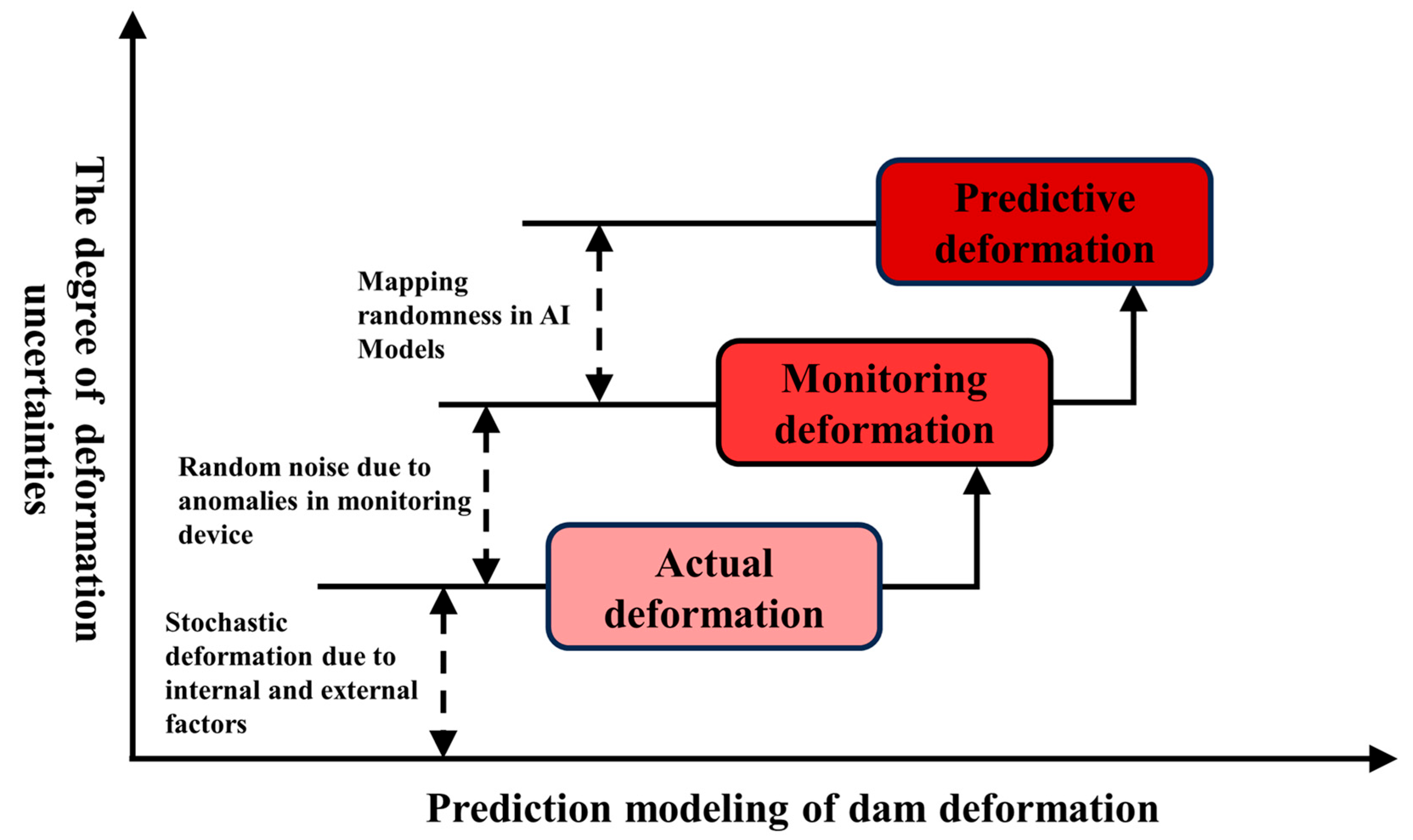
We compare the performance of point and interval predictions by mapping transformations between them. The results emphasize the importance of considering uncertainties in dam deformation prediction.
The rest of the paper is arranged as follows. After the introduction, the related theory of the proposed model is described in detail in Section 2. Section 3 provides a case study on the concrete arch dam and analyzes the results of comparison experiments. In Section 4, the necessity of considering the uncertainties in dam deformation prediction is discussed. The conclusions are summarized in Section 5.

2. Methodologies

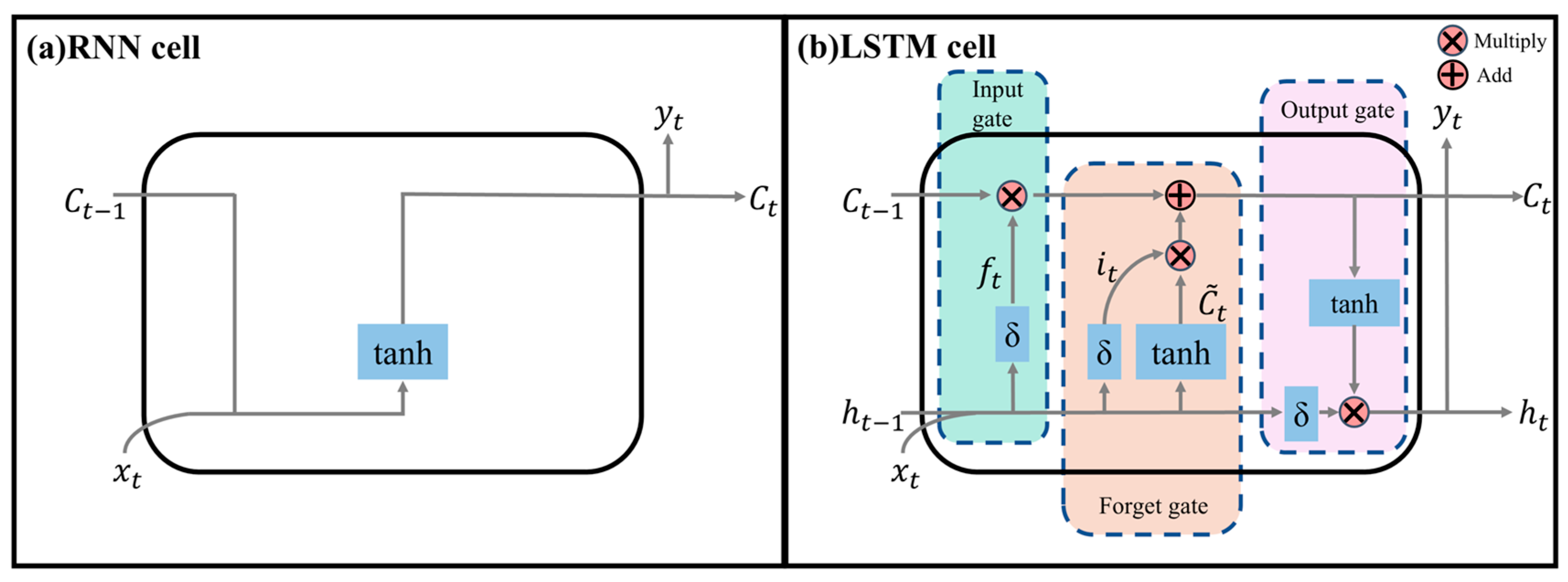
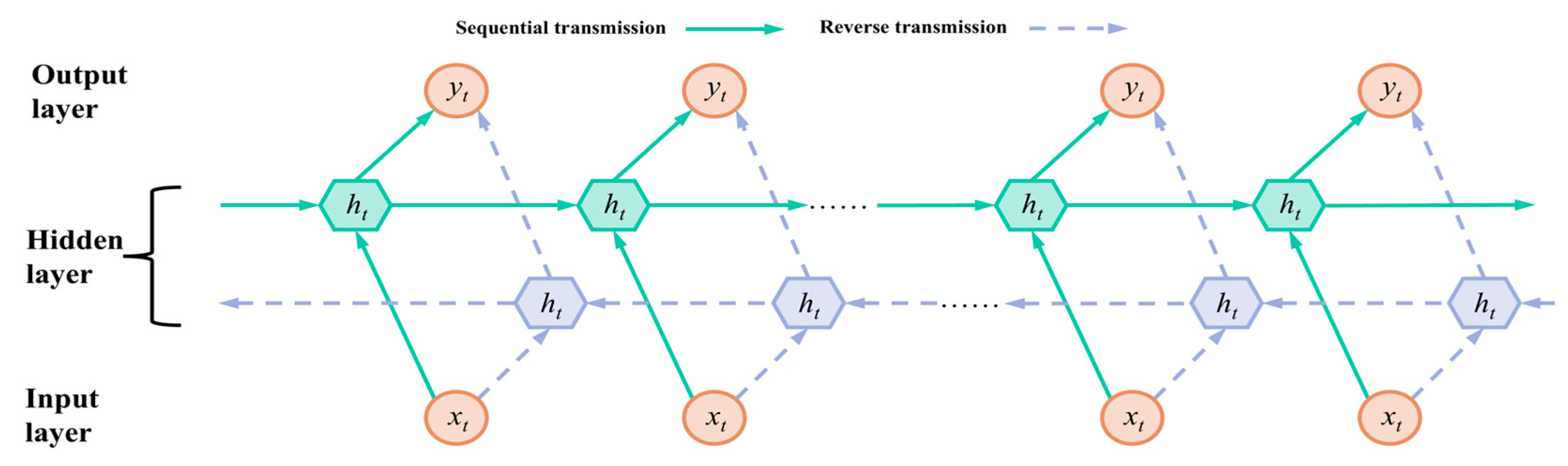
2.1. Bi-Directional Long Short-Term Memory Network

RNN was once the best AI algorithm for solving time-series prediction problems because of its ability to convey hidden layer state information [29]. However, researchers have gradually found that the single structural framework of RNN with unreasonable algorithmic solution logic easily leads to problems such as the loss of prior information and gradient explosion when dealing with complex long-term sequences [29,30]. To overcome the drawbacks of RNN, LSTM was proposed [31]. Figure 2 shows the internal unit structure of RNN and LSTM. Compared with RNN, LSTM replaces the recurrent hidden layer inside the RNN with a memory block. This memory block contains an input gate, an output gate, a forget gate, and a memory cell, and it controls the inflow and outflow of information at the hidden level through the synergy of these gate structures with the memory cell [32]. The main computational flow of LSTM is as follows:
Input   gate   calculation :   i t = σ ( W i h t 1 , x t + b i )
C ˜ t = t a n h ( W c [ h t 1 , x t ] + b c )
Forget   gate   calculation :   f t = σ ( W f [ h t 1 , x t ] + b f )
Update   cell   state :   C t = f t C t 1 + i t C ˜ t
Output   gate   calculation :   O t = σ ( W o h t 1 , x t 1 + b o )
h t = O t t a n h ( C t )
In Equations (1)–(6), C ˜ t and i t together form the input gate structure; the inflow of information controlled by the forget gate depends mainly on the relationship between the input variables x t at the current moment and the hidden state h t 1 at the previous moment; the amount of information contained in the latest cell state is determined by C ˜ t , i t , and f t ; finally, the hidden state of the current moment h t is obtained by the calculation of the output gate; b c , b i , b f , and b o represent the bias vectors of input gate, forget gate, latest cell state, and output gate, respectively; W i , W c , W f and W o are the corresponding weight matrices.
As a special variant of LSTM, the proposed Bi-LSTM has two LSTM layers with different orientations in the memory block to process information from the past and the future [33]. Figure 3 illustrates the structure of the Bi-LSTM. The two LSTM layers contain a pair of anisotropic temporal hidden states, i.e., forward h t and backward h t ,
h t = L S T M ( h t 1 , x t , c t 1 ) , t 1 , T
h t = L S T M ( h t + 1 , x t , c t + 1 ) , t 1 , T
H t = [ h t , h t ]
where T is the span of the time sequences.

2.2. Split Conformal Quantile Prediction

SCQP is an interval prediction method proposed by Romano et al. (2022) based on Split conformal prediction (SCP) [34,35]. The method inherits the advantages of conventional SCP and is able to construct PIs without any prior distribution [36]. Moreover, the addition of the pinball loss function also solves the defect of SCP that relies too much on the accuracy of the point prediction model. This approach requires splitting the training samples into a training subset indexed by L 1 and a calibration subset indexed by L 2 . The regression algorithm M q integrates pinball loss function and sets the minimization function loss as the objective. The two curves q ^ α U B and q ^ α L B that represent the upper and lower bounds of the PIs are fitted thus:
q ^ α L B = q α ( x ; θ ^ ) , q ^ α U B = q α ( x ; θ ^ ) M q ( ( X i , Y i ) : i L 1 ) θ ^ = arg min θ = 1 n i = 1 n ρ α ( Y i , q α ( X i ; θ ^ ) ) + L ( θ )
where ρ α ( Y i , q α ( X i ; θ ^ ) ) represents the pinball loss function, which can also be written as:
ρ α ( y ; z ) = ( 1 α ) ( y z ) , y z α ( y z ) , z < y
In the next key step, the consistency score E i can be calculated using the calibration set L 2 and the fit function of the upper and lower bounds, by which the error between the prediction interval P I α ( x ) = q ^ α L B = q α ( x ; θ ^ ) , q ^ α U B = q α ( x ; θ ^ ) and the actual observed value Y i can be quantified thus:
E i = max q ^ α L B ( X i ) Y i , Y i q ^ α U B
From Equation (14), it is not difficult to explore the meaning of the consistency score E i . When the observed value Y i lies below the PIs, Y i < q ^ α L B ( X i ) , E i = q ^ α L B ( X i ) Y i can be expressed as the error between the PI and the observed value. Similarly, if the observed value Y i lies above the PIs, Y i > q ^ α U B ( X i ) , then the error between PIs and the observed value Y i can be expressed as E i = q ^ α L B ( X i ) Y i . In addition, if Y i always lies within the PI, q ^ α L B ( X i ) < Y i < q ^ α U B ( X i ) , then E i will be chosen from the largest non-positive number.
So far, given the new input variable X n + 1 , the PIs of the response variable Y n + 1 can be described:
P I α ( X n + 1 ) = [ q ^ α L B ( X n + 1 ) Q 1 α ( R , L 2 ) , q ^ α L B ( X n + 1 ) + Q 1 α ( R , L 2 ) ]
Q 1 α ( E , L 2 ) : = ( 1 α ) ( 1 + 1 / L 2 ) th   empirical   quantile   of   E i : i L 2

2.3. The Evaluation Indicators of Model Performance

In this paper, the point prediction performance of the model is evaluated by three metrics: the correlation coefficient (R2), mean absolute error (MAE), and root mean square error (RMSE). These indicators can be expressed as follows:
R 2 = 1 i = 1 n ( y i y ^ i ) 2 i = 1 n ( y i y i ¯ ) 2
M A E = 1 n i = 1 n | y i y ^ i |
R M S E = 1 n i = 1 n ( y i y i ^ )
where y ^ i denotes the predicted value, y i is the actual value, and n is the total length of the sample. For MAE and RMSE, the smaller their values, the better. The range of R2 is between 0 and 1, with higher values indicating that the fitted displacements of the model are closer to the observed displacements. R2 reflects the model’s fitting performance for deformation trends, while MAE and RMSE indicate the model’s ability to control local and global error.
Similar to the point prediction model, the interval prediction model also has specific evaluation indicators. Prediction interval effective coverage (PICP) and average interval coverage width (MPIW) tend to best visualize the accuracy and effectiveness of PIs. They are defined as, respectively:
P I C P = 1 n t = 1 n k t
M P I W = 1 n t = 1 n ( U B i α L B i α )
where n is the number of target samples. k t is 1 if the samples fall within the PIs, otherwise k t is 0. U B i α and L B i α denote the upper and lower bounds of the PIs, respectively; α is the error coverage.
However, in most cases, PICP and MPIW are two opposing evaluation metrics. It is difficult for interval prediction models to maintain a balance between high PICP and small MPIW in constructing PIs. To validate the quality of the deformation PIs constructed by our proposed method, we use an evaluation metric called coverage width-based criterion (CWC), which assesses the comprehensive quality of PIs as follows:
C W C = M P I W 1 + γ ( P I C P ) exp ( η ( μ P I N C ) )
γ ( P I C P ) = 1 , P I C P < μ 0 , P I C P μ
where η and μ are the penalty parameter and the PINC of constructed PIs, respectively. When the PICP is lower than μ , the effective coverage rate of the PIs does not meet the predetermined probability requirement; then, γ ( P I C P ) = 1 . The CWC will be determined by the PICP and MPIW together; on the contrary, if the PICP is higher than μ , the effective coverage rate of the PIs meets the requirement, and the CWC is only related to MPIW. The η will be set to 10 in this paper [21].

2.4. The Proposed Bi-SCQLSTM for Dam Deformation Interval Pre Diction

Based on the theoretical background described above, this section proposes a novel distribution-free dam deformation interval prediction model that integrates Bi-LSTM with the SCQP, termed the Bi-SCQLSTM. The Bi-LSTM architecture can convey hidden states in different time dimensions and deeply explore the nonlinear feature of dam deformation. On the other hand, the SCQP algorithm generates high-quality deformation PIs that meet both high valid coverage and ideal interval coverage width, which can fully adapt to dam deformation sequences with different distributions.
The proposed Bi-SCQLSTM model is described in detail and shown in Algorithm 1, and the framework of the proposed model is summarized in Figure 4:
Algorithm 1: Procedure of Bi-SCQLSTM
Input:
    Observation dataset ( X i , Y i ) s × , 1 i n .
Set:
    Error coverage level α ( 0 , 1 ) .
Process:
    1. Divide the observation dataset ( X i , Y i ) : 1 < i < n into two disjoint subsets, the training set L 1 and the calibration set L 2 .
    2. Two function curves q ^ α L B , q ^ α U B are fitted by using a Bi-LSTM coupled with pinball loss.
    3. The consistency score E i corresponding to a finite number of samples Y i on the calibration set L 2 is calculated by Equation (20).
    4. Compute Q 1 α ( E , L 2 ) = ( 1 α ) ( 1 + 1 / L 2 ) th   empirical   quantile   of   E i : i L 2 .
Output:
    The prediction interval of the response variable Y n + 1 corresponding to the independent variable P I α ( X n + 1 ) = [ q ^ α L B ( X n + 1 ) Q 1 α ( R , L 2 ) , q ^ α L B ( X n + 1 ) + Q 1 α ( R , L 2 ) ]
(1)
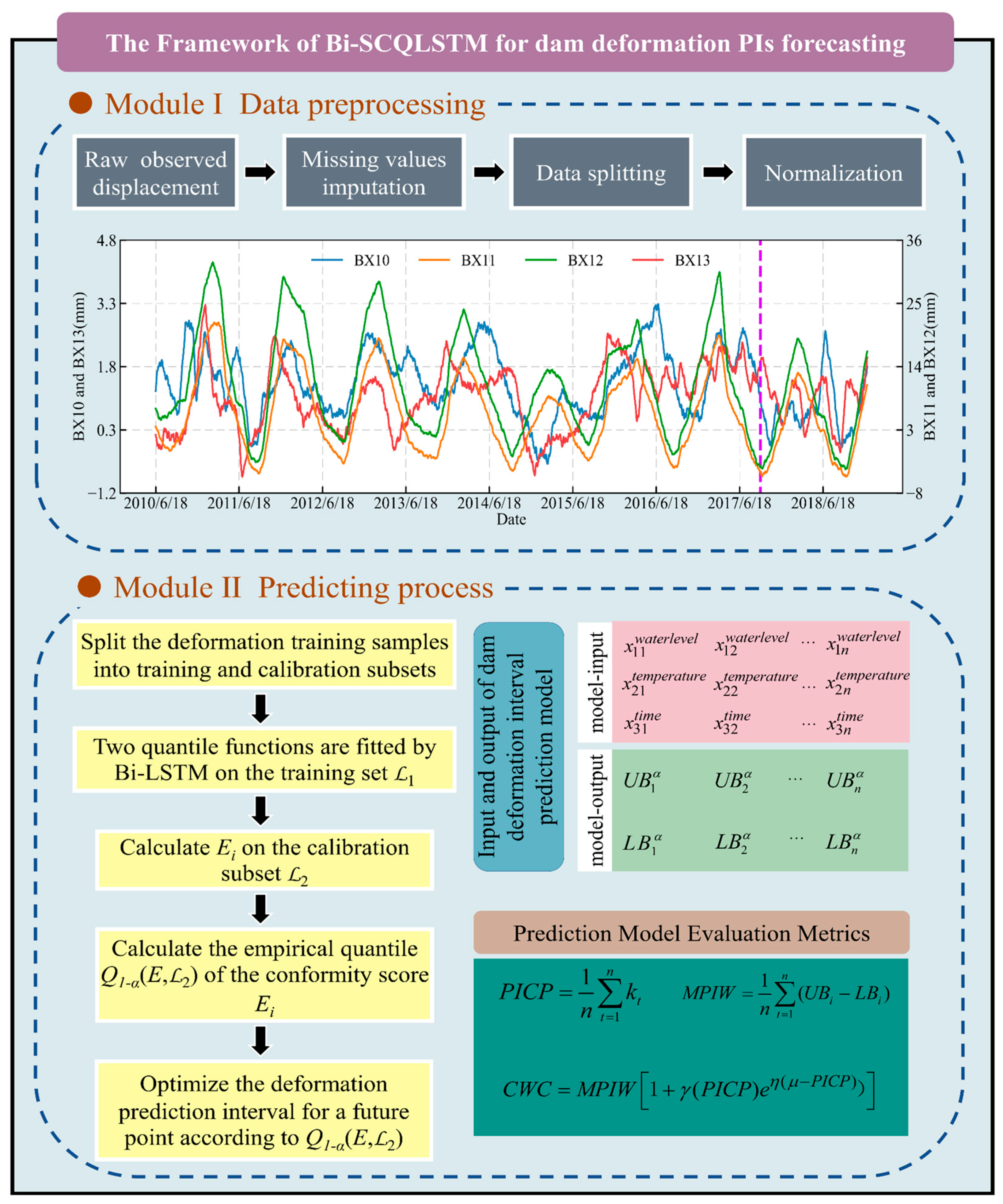
First, a raw dam monitoring series is interpolated, and the resulting dataset is divided into training samples and test samples, and min–max normalization is performed on the two sample sets independently.
(2)
Secondly, the training samples are used as the input data of the Bi-SCQLSTM. During this process, the training samples are further divided into two disjoint subsets, a training subset L 1 and a calibration subset L 2 . Two function curves q ^ α U B and q ^ α L B are fitted to the training subset L 1 using the Bi-LSTM. The number of neurons in the output layer of the Bi-LSTM is set to 2, and the cost function is defined as pinball loss. The main idea behind this process stems from quantile regression.
(3)
The Bi-LSTM is then used as the underlying evaluator for the SCQP algorithm, which is used to calculate the consistency score E i . For finite samples Y i from the calibration subset L 2 , the consistency score E i and corresponding empirical quantile Q 1 α ( R , L 2 ) will be obtained by Equation (14) and Equation (16), respectively. Then, the deformation PIs constructed by the model for the new exogenous variable X n + 1 will be optimized by the Q 1 α ( R , L 2 ) to further adapt to the dam deformation series with variance variability and random fluctuation.
(4)
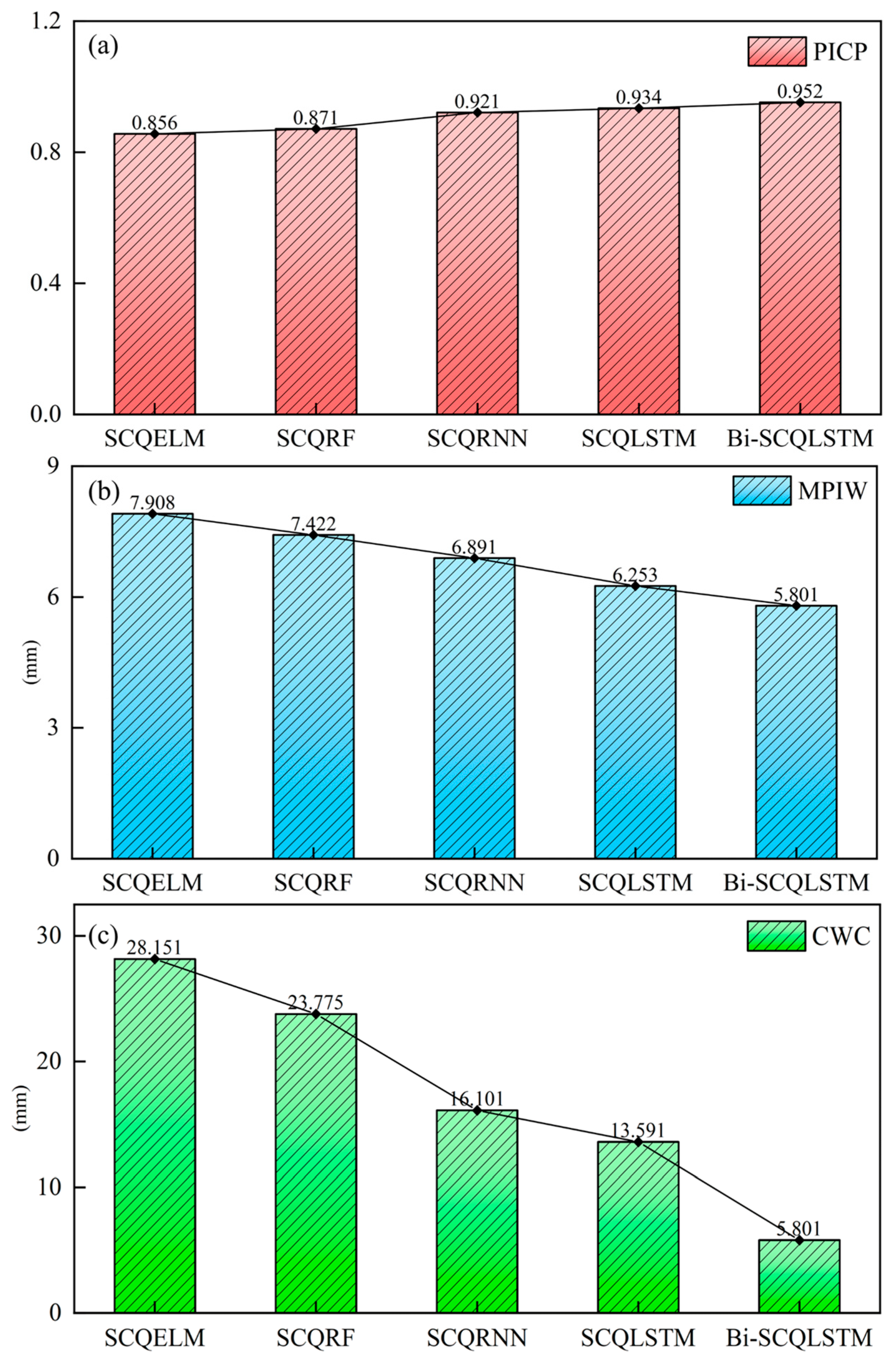
Finally, the deformation PIs are evaluated and compared by using the interval evaluation indicators PICP, MPIW, and CWC.

3. Case Study

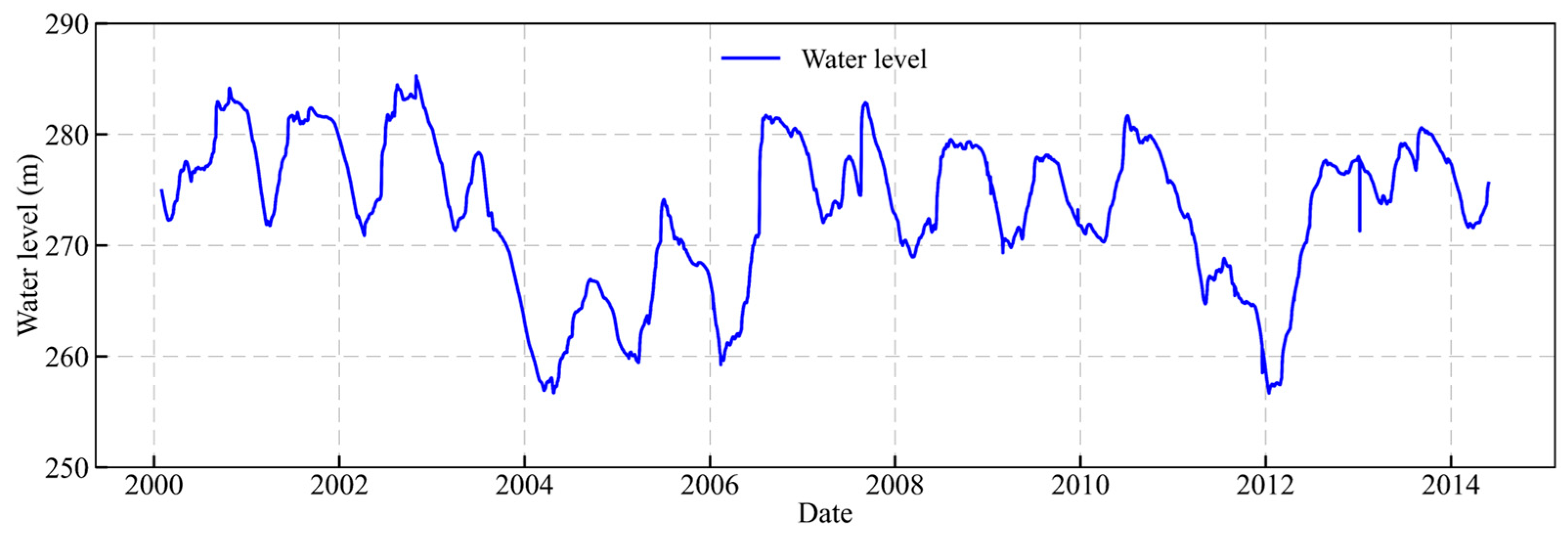
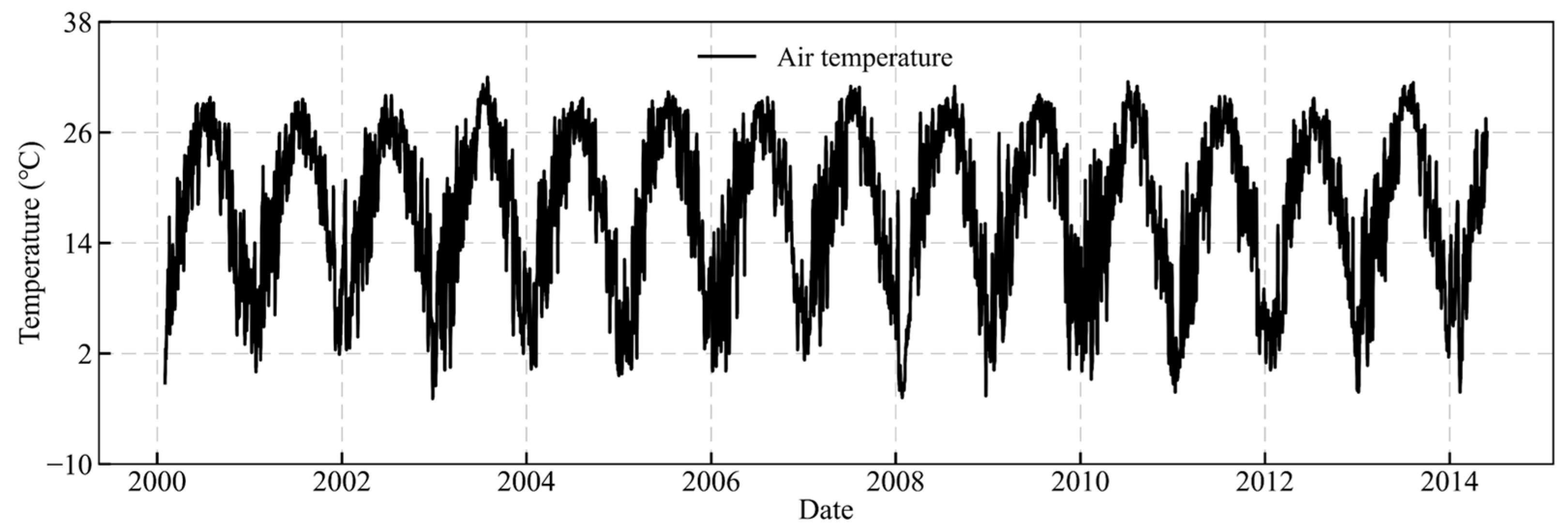
3.1. Overview of the Arch Dam Project

The proposed interval prediction model is validated with historical monitoring data from an arch dam located in south-central China. The construction of the arch dam began at the end of 1958, and the first phase was completed by the end of 1992. The major engineered task of this arch dam is flood control, but it also delivers water supply, power generation, and other associated functions. The dam has a height of 157 m, a base width of 35 m, a crest width of 7 m, a central crest arc length of 438 m, and an installed capacity of 500,000 kilowatts. Figure 5 shows the downstream area of the dam and the surrounding environment (https://www.dongjianghu.com/, accessed on 11 November 2024).
The horizontal deformation of the dam is measured using the pendulum method. In this study, the horizontal displacement (i.e., L5H291R) measured at an elevation of 291 m by pendulum L5, located on the crown cantilever of Dam Block 15, is selected as the dataset for modeling [37]. The position of the pendulum is shown in Figure 6. The selected dataset covers a total of 341 deformation observations of the arch dam from June 2000 to May 2014 (see Figure 7). These data contain 274 training samples and 67 test samples. The monitoring curves of the dam’s environmental variables, including upstream reservoir water level and temperature, are shown in Figure 8 and Figure 9.

3.2. Model Construction and Deformation Feature Selection

In order to eliminate the influence of different dimensionalities between variables and to improve the learning speed of the neural network, the training and test samples are first subjected to Min-Max Normalization before being inputted to the model, calculated as follows:
x n o r m = x min ( x ) max ( x ) min ( x )
For AI-based models, hyperparameter selection is a crucial part of the modeling process and can directly affect the performance of the prediction model. All model hyper-parameter choices involved in this study were derived by trial-and-error and grid search methods. First, we used the trial-and-error method to identify the approximate range of specific parameters. This process involved manually testing various parameter combinations and recording the fluctuations in model performance. Subsequently, grid search was employed to determine the optimal hyperparameter combination, ensuring that the model’s performance met the expected standards. Take the proposed Bi-SCQLSTM as an example. The number of bidirectional LSTM layers was set as 3, and the number of neurons was 128, 64, and 32, respectively. To prevent overfitting, a dropout layer was provided between the bidirectional LSTM layers, and the probability of each layer was selected as 0.35. The number of epochs was set to 3000; the batch size was 100; the Adam optimized learning rate was set to 0.003. The size of the sliding time window was 6, meaning that the data from the previous 6 days are used to predict the deformation of the subsequent day. In addition, considering the required accuracy of dam deformation prediction, the PINC in this study was specified for 95%.
Generally speaking, the causes of dam deformation can be divided into three main categories: deformation caused by hydrostatic pressure Y H ; deformation caused by temperature stress Y T ; and deformation caused by ageing Y t . For horizontal deformation, the deformation caused by hydrostatic pressure Y H shows a linear relationship with the upstream water level H , H 2 , H 3 , and H 4 . Thus, Y H can usually be expressed as a quadratic polynomial in terms of the upstream water level. The horizontal deformation Y t due to the time effect can usually be expressed as a combination of the monitoring date t and a function of its corresponding logarithm. Notably, Kang et al. (2020) verified that the deformation lag due to temperature effects in dams is better captured by actual historical temperature measurements, resulting in more physically explanatory dam deformation prediction [38]. Therefore, the deformation input features used in this study are based on the improved HTT statistical model:
deformation   input   factors = x w a t e r l e v e l , x t e m p e r a t u r e , x t i m e = H , H 2 , H 3 , H 4 , T 0 , T 1 2 , T 3 7 , T 8 15 , T 16 30 , T 31 60 , T 61 90 , T 91 120 , T 121 180 , δ , ln δ
where T 0 denotes the mean air temperature on the initial deformation monitoring date; T a b is the mean air temperature from days a to b ; and δ is the cumulative number of days from the initial deformation monitoring date.

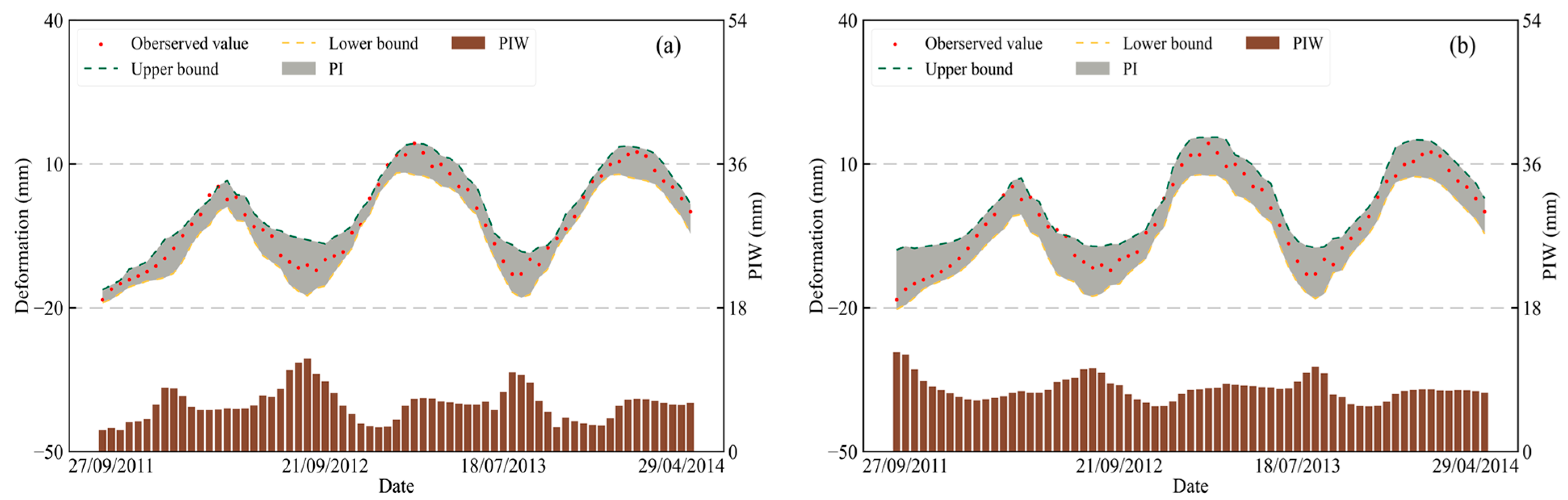
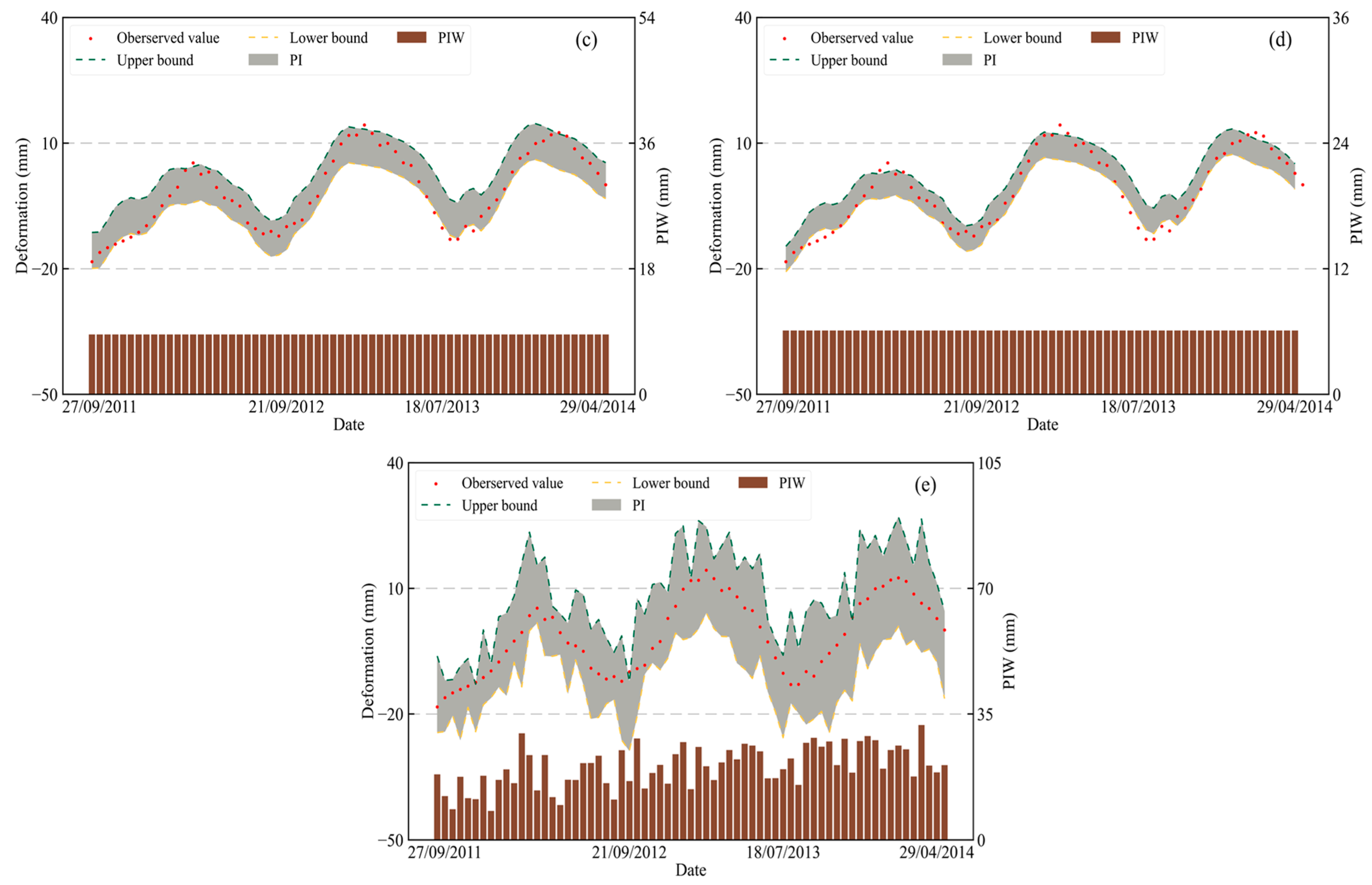
3.3. Comparative Analysis of Different Interval Prediction Models

3.3.1. Interval Prediction Performance of SCQP

This comparative experiment primarily validates the superiority and effectiveness of SCQP over other interval prediction methods for dam deformation prediction. In addition to the proposed Bi-SCQLSTM, the baseline models involved in the experiment include SCP, QR, Confidence Interval Estimation (CIE), and GPR. For the SCP, QR, and CIE methods, the base regressor is set to Bi-LSTM. Figure 10 illustrates the prediction results of different interval methods on L5H291R. The evaluation results of the deformation PIs constructed by these models are presented in Table 1.
It can be observed in Figure 10 that the PIs constructed by the Bi-SCQLSTM and the Bi-QLSTM are significantly different from other models. The coverage widths of these PIs show dynamic changes according to the actual dam deformation process. In practice monitoring experience, the peaks and troughs often imply sudden deformation due to changes in external environmental factors. Consequently, deformation uncertainty is more pronounced in these periods. The prediction results of the Bi-SCQLSTM indeed conform to this feature (the width of the interval coverage at the peaks and troughs is significantly larger than in other periods), which illustrates that the proposed model can adequately accommodate the non-homogeneous uncertainties of deformation and construct the corresponding PIs.
As can be seen in Table 1, the deformation PIs constructed by the Bi-SCQLSTM are more consistent with the criteria of high-quality PIs than those constructed by other interval prediction methods. The PICP of the Bi-SCQLSTM model is 0.951, while the MPIW is only 5.815 mm The Bi-SCQLSTM achieves the smallest CWC among five models, namely 5.815 mm. These results demonstrate that our proposed Bi-SCQLSTM strikes a delicate balance between effective coverage and interval coverage width and applies to the dam deformation data of different distribution types. Thanks to the quantile pinball loss, the proposed model can generate high-confidence PIs that satisfy the PINC and reflect the heterogeneous uncertainties of dam deformation processes under the influence of combined factors through the adaptive change of the width of PIs. On the other hand, the SCP algorithm enables the Bi-SCQLSTM to further reduce the coverage width of the dam deformation PI by identifying abrupt changes within the samples while still ensuring that the effective coverage rate meets the standard. This allows the generated deformation PIs to more closely adhere to high-quality standards.
It is worth noting that although the PIs constructed by GPR satisfy the PINC in terms of PICP as high as 0.986, the consequence of over-pursuing the effective coverage is reflected in having the high MPIW, which are 18.429. The PIs that are too wide are not conducive to quantifying the uncertainties in dam deformation, and therefore the confidence in these deformation PIs is not satisfactory.
Table 2 presents the computation times for different interval prediction models. Among them, GPR exhibits the lowest computational complexity and the shortest runtime, taking only 20.932 s. This is followed by the CIE and Bi-SCLSTM models, which are based on point prediction, with computation times of 28.024 s and 28.513 s, respectively. On the other hand, the Bi-SCQLSTM and Bi-QLSTM, which are based on quantile loss, have the highest computational complexities, requiring 32.261 s and 32.094 s, respectively. From the perspective of computational efficiency, the Bi-SCQLSTM does not demonstrate a significant advantage (GPR improves computational efficiency by 35.117% compared to the Bi-SCQLSTM). However, the CWC of the Bi-SCQLSTM is 68.451% higher than that of GRP. In dam operation and maintenance, the accuracy of a prediction model often determines whether potential safety risks in the target structure can be accurately and promptly identified. Therefore, the performance improvement brought by the Bi-SCQLSTM, at the cost of some computational efficiency, is worthwhile.

3.3.2. Comparison of Machine Learning (ML) and Deep Learning (DL) Models

In this section, four commonly utilized AI regression algorithms will be chosen to construct SCQP-based models for comparison with the Bi-SCQLSTM. These algorithms will be used. These models are split conformal extreme learning machine (SCQELM), split conformal random forest (SCQRF), split conformal recurrent neural network (SCQRNN), and split conformal long-short term memory (SCQLSTM). Figure 11 compares the visualization results of the Bi-SCQLSTM with other SCQP-based models on PICP, MPIW, and CWC.
As can be seen from Figure 11, SCQELM and SCQRF perform the worst of the five models. The effective coverage of the PIs constructed by SCQELM deviates significantly from PINC, with a PICP of only 0.856, while the corresponding MPIW and CWC are 7.908 and 28.151. The performance of SCQRF slightly outperforms, with PICP reaching 0.871, while MPIW and CWC are 7.422 mm and 23.775 mm, respectively. On the contrary, SCQRNN, SCQLSTM, and the Bi-SCQLSTM based on DL algorithms all achieve satisfactory results. The average PICPs of three models all than 0.9, with the proposed Bi-SCQLSTM being the highest to 0.952. Correspondingly, its MPIW and CWC are both only 5.801 mm.
It is clear that the advantages of DL techniques in constructing dynamic regression models extend to interval prediction as well. Additionally, compared with the unidirectional deep neural network, the Bi-LSTM with different time-dimensional hidden layers can help the proposed model to explain more possible trends in dam deformation by integrating past and future information. As a result, the Bi-SQLSTM still has the best generalization ability and robustness among many SCQP-based models.

4. The Necessity of Considering the Uncertainties in Dam Deformation

In order to verify whether the interval prediction paradigm can have a positive impact on the performance of dam deformation prediction models compared to the point prediction paradigm, in this section, the deformation PIs constructed by the interval prediction models are transformed into deterministic prediction results for comparison with deterministic prediction models. The process of converting PIs into deterministic prediction results can be expressed as follows:
Y ^ ( X i ) = [ L B α ( X i ) + U B α ( X i ) 2 ]
It should be noted that the prediction results of both the Bi-SCLSTM and CIE interval prediction come from the Bi-LSTMs based on the loss function of mean square error, and therefore their results are the same and represent the point prediction model. Figure 12 demonstrates the comparison of the result curves by interval prediction methods.
According to Figure 12, the deterministic prediction results transformed from the deformation PIs are very close to the actual deformation. The R2 of the Bi-SCQLSTM and Bi-QLSTM are 0.975 and 0.952, respectively, which is significantly higher than the R2 of the Bi-LSTM and GPR (see Figure 13). Furthermore, the MAE and RMSE of the Bi-SCQLSTM are much smaller than those of the other models, only 1.003 mm and 1.316 mm, which indicates that the Bi-SCQLSTM has the best performance in both local error and overall error control. Compared with traditional point prediction models, these methods are capable of producing prediction results that are closer to the observed deformation, and the proposed Bi-SCQLSTM still demonstrates superior performance in point prediction experiments, with its advantages primarily reflected in the following two aspects. First, the Bi-SCQLSTM constructs high-quality deformation PIs that accurately capture and explain the inherent uncertainty of dam deformation under the synergistic influence of internal and external factors. In other words, the model successfully captures subtle perturbations in the periodic trends of dam deformation during training, leading to more significant improvements in MAE and RMSE compared to R2. Second, as evidenced by the MPIW of different interval prediction paradigms (Table 1), PIs constructed by the Bi-SCQLSTM exhibit significantly narrower widths than those of other models. This phenomenon can be attributed to the proposed model’s stronger robustness against the adverse effects of mapping randomness, resulting in deformation PIs with consistently shorter coverage widths. This reduction in uncertainty is also partially reflected in the output point prediction results.

5. Conclusions and Future Work

In this study, a novel interval prediction model based on the Bi-LSTM network and SCQP algorithm is proposed to explain the uncertainties in dam deformation prediction. With the aid of DL technology and interval prediction paradigm, the Bi-SCQLSTM can construct the deformation PIs to capture and quantify the inherent uncertainties associated with the structural behavior of the dam. The comparison experiments on the deformation monitoring dataset from a real concrete arch dam fully validated the applicability and superiority of the proposed interval model. The general conclusions of this study are summarized as follows:
(1)
Dam deformation data from an arch dam are selected to test the performance of the proposed Bi-SCQLSTM. The experiment results show that, compared with the current mainstream interval prediction methods, the Bi-SCQLSTM can construct deformation PIs that meet high-quality standard.
(2)
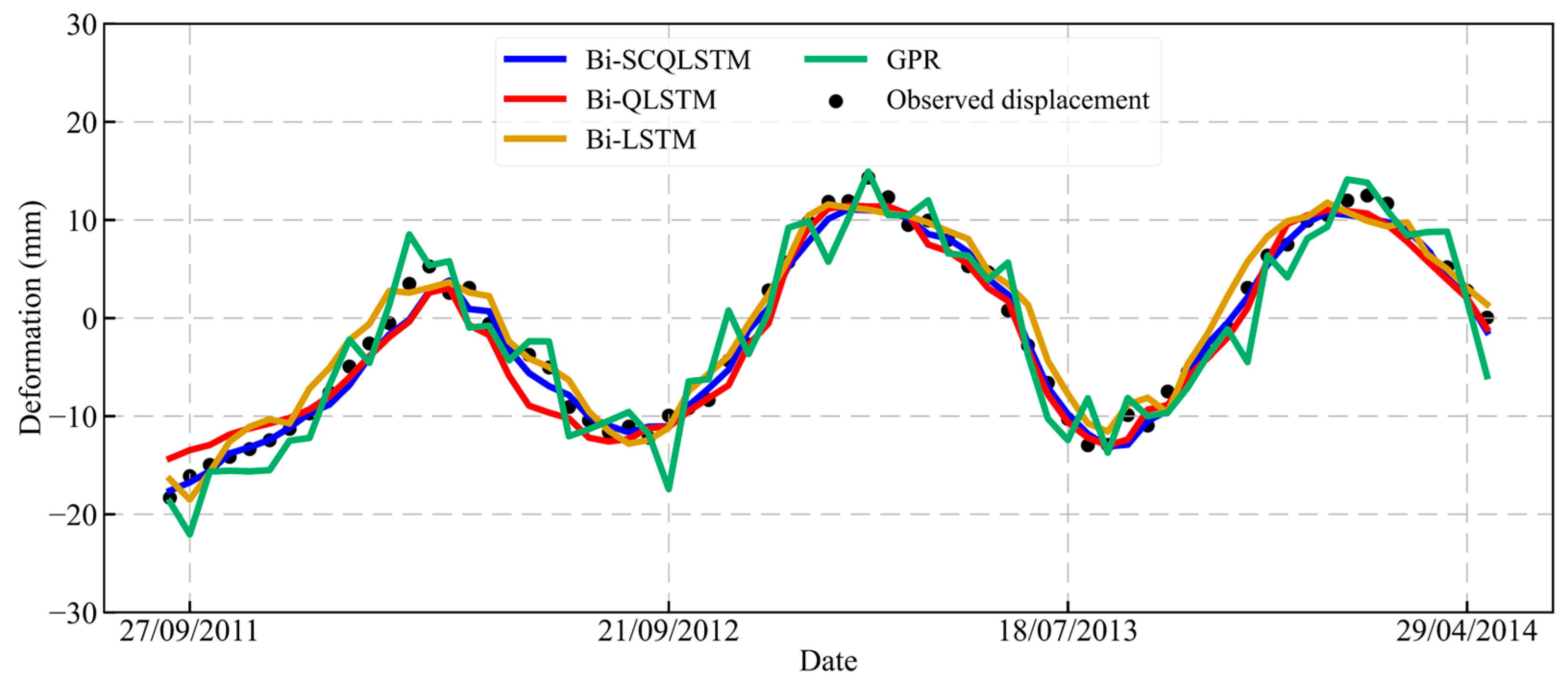
Compared to ML algorithms and unidirectional DL neural networks, the Bi-LSTM also maintains a significant advantage in interval prediction with the help of hidden layer information in different time dimensions and a larger memory threshold.
(3)
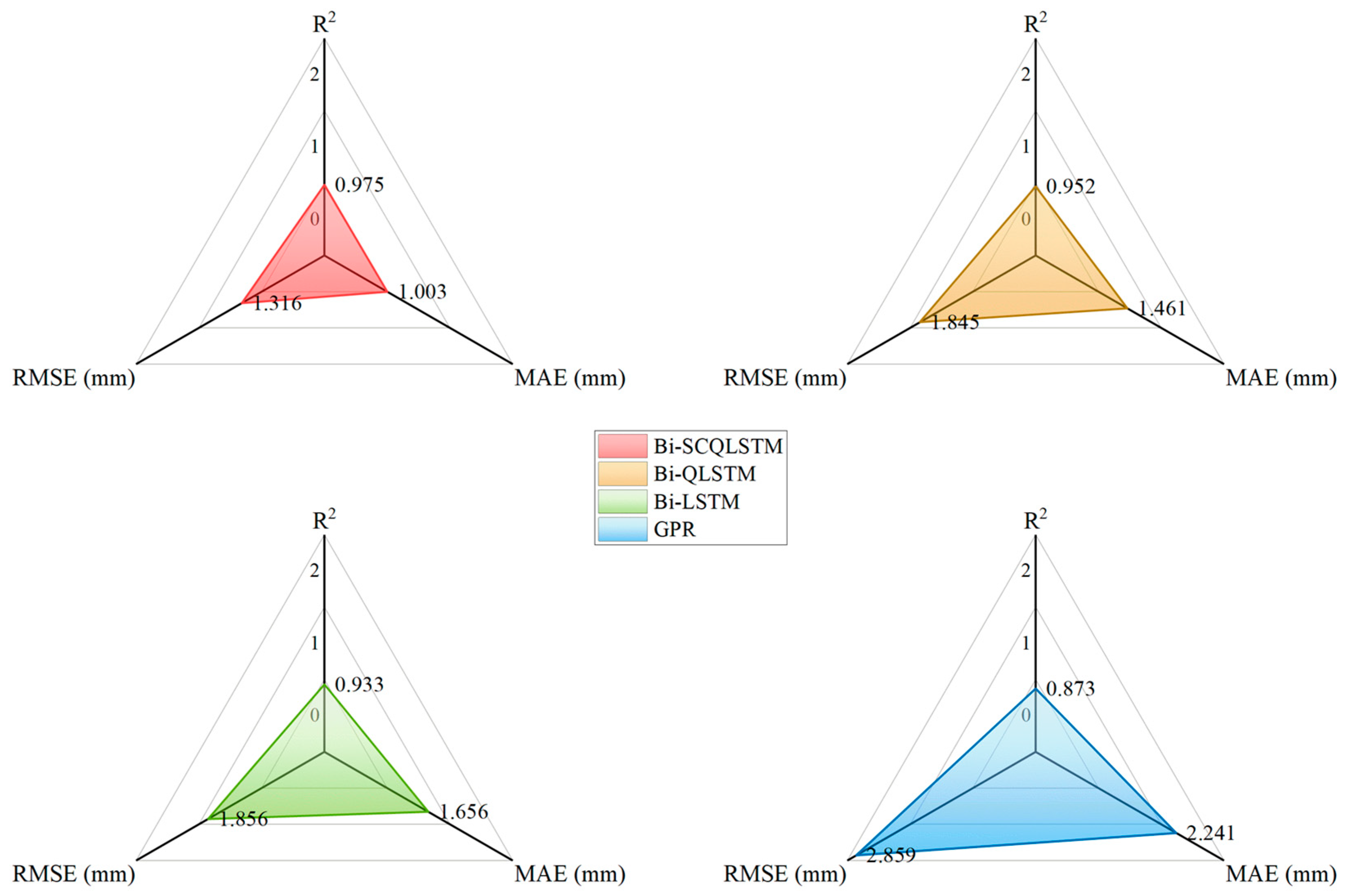
A reasonable interval prediction paradigm can reduce the prediction error due to deformation uncertainties to some extent. As a result, point prediction results transformed from PIs have higher accuracy than standard point prediction model.
Overall, the proposed Bi-SCQLSTM provides an effective scientific monitoring approach for the safe operation and maintenance of dams. By utilizing high-quality deformation PIs, the impact of uncertainty in dam deformation during specific periods can be observed. Practitioners can gain a better understanding of the potential trends in dam deformation, allowing them to develop more targeted operational strategies. These strategies can be further refined based on the degree to which uncertainty characteristics influence deformation at different times, thereby optimizing dam safety management and operational efficiency. However, it is worth acknowledging that despite its outstanding performance in dam deformation prediction, the proposed method has notable limitations. First, the model’s effectiveness needs to be thoroughly validated across a broader range of engineering cases. Second, exploring how interval prediction can be leveraged for the effective early warning of anomalous dam deformations remains a key focus of future research. Finally, the computational efficiency of the proposed model needs to be further improved.

Author Contributions

Y.S.: Contributed to the conceptualization and methodology design, conducted data analysis, and participated in manuscript drafting and revision; J.F.: Assisted in data collection and validation, provided technical support for experiments, and contributed to data interpretation; W.L. (Corresponding Author): Supervised the overall project, coordinated the research activities, contributed to the conceptualization, and revised the manuscript critically for important intellectual content.; C.L.: Responsible for conducting the experiments and preparing the original draft of the manuscript.; X.L.: Performed data curation and visualization and contributed to manuscript writing and editing; X.X.: Contributed to the formal analysis, validation, and technical review of the study. All authors have read and agreed to the published version of the manuscript.

Funding

This research was funded by the National Natural Science Foundation of China (No. 42301002 and 52109118).

Institutional Review Board Statement

Not applicable.

Informed Consent Statement

Not applicable.

Data Availability Statement

The original contributions presented in the study are included in the article, further inquiries can be directed to the corresponding author.

Acknowledgments

The author acknowledges the technical and financial support provided by the National Natural Science Foundation of China (Grant No. 42301002, and 52109118).

Conflicts of Interest

The authors declare no conflict of interest.

References

  1. Wen, Z.; Zhou, R.; Su, H. MR and stacked GRUs neural network combined model and its application for deformation prediction of concrete dam. Expert Syst. Appl. 2022, 201, 117272. [Google Scholar] [CrossRef]
  2. Ma, H.; Chi, F. Technical progress on researches for the safety of high concrete-faced rockfill dams. Engineering 2016, 2, 332–339. [Google Scholar] [CrossRef]
  3. Liu, X.; Li, Z.; Sun, L.; Khailah, E.Y.; Wang, J.; Lu, W. A critical review of statistical model of dam monitoring data. J. Build. Eng. 2023, 80, 108106. [Google Scholar] [CrossRef]
  4. Cao, W.; Wen, Z.; Su, H. Spatiotemporal clustering analysis and zonal prediction model for deformation behavior of super-high arch dams. Expert Syst. Appl. 2023, 216, 119439. [Google Scholar] [CrossRef]
  5. Cheng, L.; Zheng, D. Two online dam safety monitoring models based on the process of extracting environmental effect. Adv. Eng. Softw. 2013, 57, 48–56. [Google Scholar] [CrossRef]
  6. Ren, Q.; Li, M.; Song, L.; Liu, H. An optimized combination prediction model for concrete dam deformation considering quantitative evaluation and hysteresis correction. Adv. Eng. Inform. 2020, 46, 101154. [Google Scholar] [CrossRef]
  7. Xu, C.; Yue, D.; Deng, C. Hybrid GA/SIMPLS as alternative regression model in dam deformation analysis. Eng. Appl. Artif. Intell. 2012, 25, 468–475. [Google Scholar] [CrossRef]
  8. Li, B.; Yang, J.; Hu, D. Dam monitoring data analysis methods: A literature review. Struct. Control Health Monit. 2020, 27, e2501. [Google Scholar] [CrossRef]
  9. Su, H.; Wen, Z.; Wang, F.; Wei, B.; Hu, J. Multifractal scaling behavior analysis for existing dams. Expert Syst. Appl. 2013, 40, 4922–4933. [Google Scholar] [CrossRef]
  10. Sun, L.; Ji, Y.; Zhu, X.; Peng, T. Process knowledge-based random forest regression for model predictive control on a nonlinear production process with multiple working conditions. Adv. Eng. Inform. 2022, 52, 101561. [Google Scholar] [CrossRef]
  11. Desai, M.; Shah, M. An anatomization on breast cancer detection and diagnosis employing multi-layer perceptron neural network (MLP) and Convolutional neural network (CNN). Clin. eHealth 2021, 4, 1–11. [Google Scholar] [CrossRef]
  12. Huang, G.B.; Zhu, Q.Y.; Siew, C.K. Extreme learning machine: Theory and applications. Neurocomputing 2006, 70, 489–501. [Google Scholar] [CrossRef]
  13. Qu, X.; Yang, J.; Chang, M. A deep learning model for concrete dam deformation prediction based on RS-LSTM. J. Sens. 2019, 2019, 4581672. [Google Scholar] [CrossRef]
  14. Dai, B.; Gu, C.; Zhao, E.; Qin, X. Statistical model optimized random forest regression model for concrete dam deformation monitoring. Struct. Control Health Monit. 2018, 25, e2170. [Google Scholar] [CrossRef]
  15. Kang, F.; Liu, J.; Li, J.; Li, S. Concrete dam deformation prediction model for health monitoring based on extreme learning machine. Struct. Control Health Monit. 2017, 24, e1997. [Google Scholar] [CrossRef]
  16. Ren, Q.; Li, M.; Li, H.; Shen, Y. A novel deep learning prediction model for concrete dam displacements using interpretable mixed attention mechanism. Adv. Eng. Inform. 2021, 50, 101407. [Google Scholar] [CrossRef]
  17. Song, J.; Liu, Y.; Yang, J. Dam Safety Evaluation Method after Extreme Load Condition Based on Health Monitoring and Deep Learning. Sensors 2023, 23, 4480. [Google Scholar] [CrossRef] [PubMed]
  18. Kang, H.; Yang, S.; Huang, J.; Oh, J. Time series prediction of wastewater flow rate by bidirectional LSTM deep learning. Int. J. Control Autom. Syst. 2020, 18, 3023–3030. [Google Scholar] [CrossRef]
  19. Huang, X.; Li, Q.; Tai, Y.; Chen, Z.; Liu, J.; Shi, J.; Liu, W. Time series forecasting for hourly photovoltaic power using conditional generative adversarial network and Bi-LSTM. Energy 2022, 246, 123403. [Google Scholar] [CrossRef]
  20. Ren, Q.; Li, M.; Kong, R.; Shen, Y.; Du, S. A hybrid approach for interval prediction of concrete dam displacements under uncertain conditions. Eng. Comput. 2021, 39, 1285–1303. [Google Scholar] [CrossRef]
  21. Ren, Q.; Li, M.; Shen, Y. A new interval prediction method for displacement behavior of concrete dams based on gradient boosted quantile regression. Struct. Control Health Monit. 2022, 29, e2859. [Google Scholar] [CrossRef]
  22. Li, Y.; Bao, T.; Shu, X.; Chen, Z.; Gao, Z.; Zhang, K. A hybrid model integrating principal component analysis, fuzzy C-means, and Gaussian process regression for dam deformation prediction. Arab. J. Sci. Eng. 2021, 46, 4293–4306. [Google Scholar] [CrossRef]
  23. Hosmer, D.W.; Lemeshow, S. Confidence interval estimation of interaction. Epidemiology 1992, 3, 452–456. [Google Scholar] [CrossRef]
  24. Yang, X.; Xiang, Y.; Shen, G.; Sun, M. A Combination Model for Displacement Interval Prediction of Concrete Dams Based on Residual Estimation. Sustainability 2022, 14, 16025. [Google Scholar] [CrossRef]
  25. Jiang, J.; Zhang, W. Distribution-free prediction intervals in mixed linear models. Stat. Sin. 2002, 12, 537–553. [Google Scholar]
  26. Khosravi, A.; Nahavandi, S.; Creighton, D.; Atiya, A.F. Lower upper bound estimation method for construction of neural network-based prediction intervals. IEEE Trans. Neural Netw. 2010, 22, 337–346. [Google Scholar] [CrossRef]
  27. Jensen, V.; Bianchi, F.M.; Anfinsen, S.N. Ensemble conformalized quantile regression for probabilistic time series forecasting. IEEE Trans. Neural Netw. Learn. Syst. 2022, 35, 9014–9025. [Google Scholar] [CrossRef]
  28. Hu, J.; Luo, Q.; Tang, J.; Heng, J.; Deng, Y. Conformalized temporal convolutional quantile regression networks for wind power interval forecasting. Energy 2022, 248, 123497. [Google Scholar] [CrossRef]
  29. Yu, Y.; Si, X.; Hu, C.; Zhang, J. A review of recurrent neural networks: LSTM cells and network architectures. Neural Comput. 2019, 31, 1235–1270. [Google Scholar] [CrossRef] [PubMed]
  30. Ghimire, S.; Deo, R.C.; Casillas-Pérez, D.; Salcedo-Sanz, S.; Sharma, E.; Ali, M. Deep learning CNN-LSTM-MLP hybrid fusion model for feature optimizations and daily solar radiation prediction. Measurement 2022, 202, 111759. [Google Scholar] [CrossRef]
  31. Sherstinsky, A. Fundamentals of recurrent neural network (RNN) and long short-term memory (LSTM) network. Phys. D Nonlinear Phenom. 2020, 404, 132306. [Google Scholar] [CrossRef]
  32. Zhang, J.; Guo, X.; Zong, S.; Xu, H. Multiparameter estimation and LSTM-based prediction method for health state of single-layer reticulated shells. J. Build. Eng. 2023, 76, 107128. [Google Scholar] [CrossRef]
  33. Yan, X.; Guan, T.; Fan, K.; Sun, Q. Novel double layer BiLSTM minor soft fault detection for sensors in air-conditioning system with KPCA reducing dimensions. J. Build. Eng. 2021, 44, 102950. [Google Scholar] [CrossRef]
  34. Romano, Y.; Patterson, E.; Candes, E. Conformalized quantile regression. Adv. Neural Inf. Process. Syst. 2019, 32, 3543–3553. [Google Scholar]
  35. Lei, J.; G’sell, M.; Rinaldo, A.; Tibshirani, R.J.; Wasserman, L. Distribution-free predictive inference for regression. J. Am. Stat. Assoc. 2018, 113, 1094–1111. [Google Scholar] [CrossRef]
  36. Lin, Z.; Trivedi, S.; Sun, J. Conformal prediction with temporal quantile adjustments. Adv. Neural Inf. Process. Syst. 2022, 35, 31017–31030. [Google Scholar]
  37. Zhang, J.; Cao, X.; Xie, J.; Kou, P. An Improved Long Short-Term Memory Model for Dam Displacement Prediction. Math. Probl. Eng. 2019, 2019, 6792189. [Google Scholar] [CrossRef]
  38. Kang, F.; Li, J. Displacement model for concrete dam safety monitoring via gaussian process regression considering extreme air temperature. J. Struct. Eng. 2020, 146, 05019001. [Google Scholar] [CrossRef]
Figure 1. The uncertainties in dam deformation prediction.
Applsci 15 01960 g001
Figure 2. Internal infrastructure comparison of (a) RNN cell, (b) LSTM cell.
Applsci 15 01960 g002
Figure 3. The structure of Bi-LSTM.
Applsci 15 01960 g003
Figure 4. The framework of proposed Bi-SCQLSTM for dam deformation PI forecasting.
Applsci 15 01960 g004
Figure 5. Downstream view of the arch dam in China. (a) Side view; (b) Front view.
Applsci 15 01960 g005
Figure 6. The position of the pendulum L5.
Applsci 15 01960 g006
Figure 7. Historical monitoring deformation of L5H291R.
Applsci 15 01960 g007
Figure 8. Historical monitoring of the water level of the arch dam.
Applsci 15 01960 g008
Figure 9. Historical monitoring of the air temperature of the arch dam.
Applsci 15 01960 g009
Figure 10. 95% PIs obtained from different interval methods on L5H291R: (a) Bi-SCLSTM, (b) Bi-QLSTM, (c) CIE, (d) GPR, (e) Bi-SCQLSTM.
Applsci 15 01960 g010aApplsci 15 01960 g010b
Figure 11. The visualization results of SCQP-based models on PICP, MPIW, and CWC: (a) PICP, (b) MPIW, and (c) CWC.
Applsci 15 01960 g011
Figure 12. Point prediction results of interval prediction models.
Applsci 15 01960 g012
Figure 13. Quantitative evaluation of the point prediction performance of different models.
Applsci 15 01960 g013
Table 1. Quantitative evaluation of different interval prediction results.
Deformation Interval Prediction ModelsL5H291R
PICPMPIW (mm)CWC (mm)
Bi-SCQLSTM0.9515.8155.815
Bi-QLSTM0.9577.8537.853
Bi-SCLSTM0.8218.57739.735
CIE0.71339.735100.329
GPR0.98618.42918.429
Table 2. Computation time of different interval prediction results.
Deformation Interval Prediction ModelsComputation Time (s)
Bi-SCQLSTM32.261
Bi-QLSTM32.094
Bi-SCLSTM28.513
CIE28.024
GPR20.932
Disclaimer/Publisher’s Note: The statements, opinions and data contained in all publications are solely those of the individual author(s) and contributor(s) and not of MDPI and/or the editor(s). MDPI and/or the editor(s) disclaim responsibility for any injury to people or property resulting from any ideas, methods, instructions or products referred to in the content.

