Featured Application
This study introduces a novel hybrid method combining Genetic Programming (GP) and XGBoost to accurately predict the compression index (Cc) of clayey soils. The proposed model offers a powerful tool for geotechnical engineers to assess soil compressibility with higher precision and aids in the design and analysis of foundations, earth structures, and settlement calculations. The method’s ability to handle complex, nonlinear relationships makes it particularly valuable for projects involving diverse soil types and challenging site conditions. Its application can significantly enhance the reliability of geotechnical assessments and streamline the design process for critical infrastructure projects.
Abstract
The accurate prediction of the compression index (Cc) is crucial for understanding the settlement behavior of clayey soils, which is a key factor in geotechnical design. Traditional empirical models, while widely used, often fail to generalize across diverse soil conditions due to their reliance on simplified assumptions and regional dependencies. This study proposed a novel hybrid method combining Genetic Programming (GP) and XGBoost methods. A large database (including 385 datasets) of geotechnical properties, including the liquid limit (LL), the plasticity index (PI), the initial void ratio (e0), and the water content (w), was used. The hybrid GP-XGBoost model achieved remarkable predictive performance, with an R2 of 0.966 and 0.927 and mean squared error (MSE) values of 0.001 and 0.001 for training and testing datasets, respectively. The mean absolute error (MAE) was also exceptionally low at 0.030 for training and 0.028 for testing datasets. Comparative analysis showed that the hybrid model outperformed the standalone GP (R2 = 0.934, MSE = 0.003) and XGBoost (R2 = 0.939, MSE = 0.002) models, as well as traditional empirical methods such as Terzaghi and Peck (R2 = 0.149, MSE = 0.090). Key findings highlighted that the initial void ratio and water content are the most influential predictors of Cc, with feature importance scores of 0.55 and 0.27, respectively. The novelty of the proposed method lies in its ability to combine the interpretability of GP with the computational efficiency of XGBoost and results in a robust and adaptable predictive tool. This hybrid approach has the potential to advance geotechnical engineering practices by providing accurate and interpretable models for diverse soil profiles and complex site conditions.
1. Introduction
The compression index (Cc) is a crucial parameter in geotechnical engineering for predicting the settlement behavior of clayey soils under consolidation. Its accurate estimation is fundamental for foundation design and soil stability analysis. Conventionally, Cc is empirically estimated using correlations based on soil index properties (e.g., the liquid limit, the plasticity index) or determined directly through laboratory consolidation tests [1,2]. While these traditional methods provide useful estimations, they are often limited by regional soil characteristics and laboratory constraints [3]. Recent advancements in machine learning (ML) have enabled more accurate, adaptable predictions of geotechnical parameters like Cc [4].
Many empirical models have been developed to correlate Cc with soil properties such as the natural water content, the liquid limit, and the void ratio. Skempton [2] proposed one of the earliest models, correlating Cc with the liquid limit for normally consolidated clays.
In 1944, Skempton [2] proposed an empirical formula to estimate the Cc of remolded clay based on their liquid limit (LL):
Cc = 0.007 × (LL − 10)
This equation suggests that the compression index increases linearly with the liquid limit.
For normally consolidated clays, Terzaghi and Peck [1] recommended a similar relationship with a slightly higher coefficient:
Cc = 0.009 × (LL − 10)
These correlations provide a straightforward method to estimate the compressibility of clays using their liquid limit.
Other studies have since refined these relationships and incorporated more variables for improved accuracy [5,6]. However, empirical models are often highly dependent on soil-specific characteristics and lead to less reliable predictions across diverse soil profiles [7]. Table 1 shows the main empirical correlations for determining Cc.

Table 1.
Empirical correlations to determine Cc.
A recent study developed a novel gene expression programming (GEP) model to predict the compression index (Cc) of fine-grained soils using the liquid limit (LL), the plastic limit (PL), and the initial void ratio (e0) and provide a cost-effective and time-efficient alternative to conventional methods while demonstrating superior performance in terms of R2, the RMSE, and the MAE [12]. Another study utilized single and MLR analyses to predict the compression index (Cc) of fine-grained remolded soils using basic soil properties, such as the liquid limit (LL), the plasticity index (PI), the optimum moisture content (OMC), the maximum dry density (MDD), and the DFS. The best-proposed equations showed an R2 of 0.95 and an average variation of −13.67% to +9.62%, making it a reliable tool when combined with engineering judgment [13].
Furthermore, a study evaluated the accuracy of an artificial neural network (ANN) model for predicting the compression index (Cc) by comparing it to laboratory values and models proposed by Widodo and Singh [14]. The proposed ANN model achieved a mean target value of 0.5409 and a correlation coefficient (R2) of 0.939, and outperformed the models by Slamet Widodo (R2 = 0.929) and Amardeep Singh (R2 = 0.892). The predicted Cc values from the ANN model demonstrated a better distribution around the trend line and highlighted its superior accuracy and strong agreement with laboratory results. Also, in another study [15], artificial neural network (ANN) methodologies have been proposed as efficient alternatives to traditional 15-day consolidation tests for predicting the compression index (Cc) in fine-grained soils. Another study trained an ANN using a dataset of 560 high- and low-plasticity soil samples from Turkey, with input parameters such as the natural water content, the LL, the PL, the PI, and the initial void ratio. Using Matlab 2023a’s regression learner program, the model achieved an R2 of 0.81, demonstrating its ability to provide reliable Cc predictions with fewer experiments and significantly shorter timeframes, making it a valuable tool for geotechnical engineering.
Genetic Programming (GP) is becoming increasingly popular in geotechnical engineering because of its flexibility and ability to model non-linear relationships. It has been successfully used to predict soil properties such as shear strength, permeability, and bearing capacity [16,17,18]. Research by Pham et al. [19] and Ahmadi et al. [20] shows that GP can accurately model soil parameters, especially when traditional methods fall short. Its strength lies in its evolutionary approach where solutions adapt without needing predefined formulas. It makes this method ideal for handling complex, non-linear geotechnical data [21,22,23].
XGBoost, as a powerful gradient-boosting technique, has gained recognition for its efficiency and accuracy in analyzing large, high-dimensional datasets. It has been widely used in civil and geotechnical engineering to predict properties like soil compaction and undrained shear strength [24,25]. Studies by Pal and Deswal [26] and Ma et al. [27] demonstrated that XGBoost often outperforms traditional machine learning models due to its robust regularization features and resistance to overfitting. Additionally, its interpretability, through feature importance metrics, provides valuable insights into how soil properties influence Cc [28,29,30].
Combining GP and XGBoost into a hybrid model addresses the limitations of each standalone approach. This hybridization leverages GP’s adaptability and XGBoost’s computational power, leading to improved accuracy and reliability in predicting complex parameters like soil strength and stability under varying conditions [17,31,32]. Recent studies have shown that hybrid models significantly enhance performance and can accommodate the variability seen across different soil types and conditions, making them highly adaptable solutions for predicting Cc [33].
Comparative studies, such as those by Deng et al. [34] and Shahin et al. [35], highlight that hybrid machine learning models consistently outperform traditional methods. By combining multiple techniques, hybrid models handle non-linear relationships more effectively and reduce prediction errors for parameters like Cc [36]. Despite these advancements, challenges remain in generalizing these models across various soil profiles and conditions. Further research is needed to validate their applicability in diverse geotechnical settings [29,37]. Additionally, incorporating interpretability techniques, like SHAP (SHapley Additive exPlanations), could further clarify the relationship between soil properties and Cc, improving their acceptance in practice [38,39,40].
This paper explores the use of GP, XGBoost, and their hybrid model to predict Cc using a comprehensive geotechnical database, and demonstrates their potential in advancing soil behavior prediction.
The proposed method fills critical gaps in the prediction of the compression index (Cc) of fine-grained soils by addressing the limitations of traditional consolidation testing and empirical models. Conventional methods for determining Cc are time-consuming, requiring up to 15 days for test preparation, execution, and parameter calculation, which can significantly delay construction projects. Empirical formulas, while useful for initial estimates, often fail to generalize across diverse datasets due to their reliance on simplified assumptions and limited variables. These challenges underscore the need for advanced, efficient methodologies capable of delivering accurate and reliable Cc predictions while reducing time and resource demands.
To bridge these gaps, this study aims to develop and validate a novel hybrid machine learning model combining Genetic Programming (GP) and XGBoost. This hybrid approach uses the interpretability of GP and the computational efficiency of XGBoost to accurately predict Cc using easily measurable soil properties such as the liquid limit (LL), the plasticity index (PI), the initial void ratio (e0), and the water content (w). The research seeks to overcome the shortcomings of traditional methods by creating a model that not only delivers superior predictive accuracy but also generalizes effectively across diverse soil profiles. By validating the hybrid model against standalone GP and XGBoost models, as well as traditional empirical approaches, the study provides a robust and adaptable tool for geotechnical engineers, enabling faster, more cost-effective, and more reliable predictions of soil behavior.
2. Materials and Methods
2.1. Database
The database (including 352 sets of data) used in this study includes a detailed collection of geotechnical data focused on the properties of clay soils related to the prediction of the compression index (Cc). The key parameters in the database are the initial void ratio (e0), the liquid limit (LL), the plasticity index (PI), and the water content (w). This database was collected from Alhaji et al. [41]; Benbouras et al. [42]; McCabe et al. [43]; Mitachi and Ono [44]; Widodo and Ibrahim [45]; and Zaman et al. [46].
These parameters were carefully chosen for their critical role in the understanding and prediction of soil compressibility. The liquid limit reflects the clay mineralogy and water-holding capacity and directly impacts compressibility during consolidation. The plasticity index indicates the range of moisture content where the soil remains plastic and correlates with its deformation potential under load. The initial void ratio measures soil structure and density. This parameter plays a fundamental role in determining how much soil will compress. Studies by experts like Skempton [2], Terzaghi and Peck [1], and others have confirmed the importance of these parameters in empirical models for estimating Cc. Beyond theory, they are practical for field investigations as they can be measured using standard laboratory methods. Together, these parameters provide a great and strong foundation for integrating established soil mechanics principles with advanced predictive modeling techniques.
In this study, an 80/20 train-test split was used, selected through a random sampling process with a fixed seed to ensure reproducibility. This ratio was chosen based on common machine learning practices, balancing the need for sufficient training data with reliable testing performance. Although no formal optimization algorithm was applied, we experimented with different splits (e.g., 70/30 and 90/10) to assess their impact on model performance. The 80/20 split consistently provided stable and accurate results. Additionally, 5-fold cross-validation was employed to enhance model robustness and mitigate the effects of data splitting bias.
Table 2 shows the full database, which includes 352 observations with Cc values ranging from 0.050 to 1.64 and a mean of 0.241. Table 3 focuses on the training subset with 282 observations and shows a slightly higher mean Cc of 0.244. Table 4 highlights the testing subset of 70 observations with a slightly lower mean Cc of 0.230 and narrower parameter ranges. These metrics reflect consistent patterns across the subsets, essential for building reliable predictive models. The complete database is presented in Appendix A.
Table 2.
Statistical metrics for the complete dataset used in predicting Cc.
Table 3.
Statistical metrics for the training dataset used in predicting Cc.
Table 4.
Statistical metrics for the testing dataset used in predicting Cc.
Figure 1 shows the Pearson correlation coefficients between key variables: the liquid limit (LL), the plasticity index (PI), the initial void ratio (e0), the water content (w), and Cc. Pearson correlation measures the strength of the linear relationship between two variables, with values ranging from −1 to +1. A value of +1 means a perfect positive relationship, −1 indicates a perfect negative relationship, and 0 means no linear relationship.
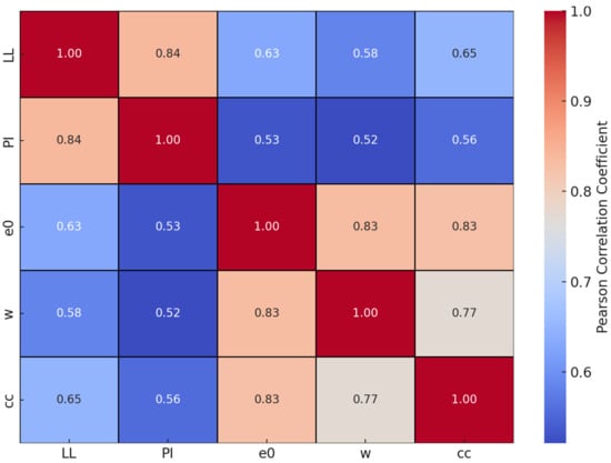
Figure 1.
Pearson correlation heatmap of variables influencing Cc.
In the heatmap, strong correlations are shown in red, while weaker ones appear in blue. The strongest connections with Cc are seen for e0 and w, with coefficients of 0.83 and 0.77, respectively. The LL and the PI also show moderate correlations at 0.65 and 0.56, which is expected due to their inherent mathematical relationship (PI = LL − PL). While no feature was removed to maintain the physical relevance of the geotechnical parameters, this dependency was acknowledged as a limitation in the study. These findings highlight that e0 and w are the most influential factors in predicting Cc.
To prepare the dataset for analysis, data cleaning steps such as outlier removal using Z-scores () and missing value imputation were conducted.
Normalization was applied to scale the data between 0 and 1, ensuring uniformity:
This ensures that all variables contribute equally to model training.
To improve the quality of the dataset and enhance the robustness of the predictive models, outlier detection and removal was conducted using the Boxplot method, a widely used statistical technique based on the interquartile range (IQR). This method helps to identify data points that deviate significantly from the central distribution, which could otherwise negatively impact model performance.
The Boxplot method identifies outliers using the following criteria:
where, Q1 = the first quartile (25th percentile), Q3 = the third quartile (75th percentile), and IQR = the interquartile range (Q3 − Q1)
Lower Bound = Q1 − 1.5 × IQR
Upper Bound = Q3 + 1.5 × IQR
Data points falling below the lower bound or above the upper bound were considered outliers. This method was applied to all continuous input features, including the liquid limit (LL), the plasticity index (PI), the initial void ratio (e0), the natural moisture content (w), and the fines content.
The outlier removal procedure involved four key steps to ensure data consistency and improve model performance. First, boxplots were generated for each feature to visualize data distribution and detect extreme values. Next, outliers were identified using the interquartile range (IQR) thresholds, which helped in pinpointing data points that deviated significantly from the norm. These identified outliers were then removed from the dataset to minimize the risk of skewed model predictions. Finally, the dataset was re-evaluated to confirm the absence of any remaining influential outliers that could bias the models. The impact of outlier removal was significant, as it enhanced model accuracy by reducing the influence of extreme values, improved generalization capability by ensuring the model was trained on data representative of typical geotechnical conditions, and stabilized the feature importance rankings, leading to more reliable interpretations of the factors affecting the compression index (Cc).
In this study, GP and XGBoost were selected based on their complementary strengths in handling complex, non-linear relationships inherent in geotechnical datasets. GP excels at generating interpretable symbolic regression models, providing insights into the mathematical relationships between soil properties and the compression index (Cc). XGBoost, on the other hand, is a robust ensemble learning algorithm known for its high predictive accuracy, scalability, and ability to handle non-linear feature interactions effectively.
2.2. Multiple Linear Regression (MLR)
Multiple linear regression models the relationship between input features and the target variable (Cc) by assuming a linear relationship. The general formula for a multivariate linear regression model is as follows:
where Cc: the compression index, Xi: the input features (e.g., e0, the LL, the PI), β0, βi: coefficients determined via least squares, and ϵ: the error term
The model’s coefficients were calculated by minimizing the residual sum of squares (RSS):
where Cc,i: the actual compression index, and : the predicted compression index.
Multiple linear regression (MLR) is often used as a baseline model to explore the simplest relationships in the data. Its performance is evaluated using metrics like the coefficient of determination (R2), the mean squared error (MSE), and the mean absolute error (MAE). R2 indicates how much of the variation in the dependent variable is explained by the independent variables, with values closer to 1 showing a better fit.
The MSE measures the average squared difference between the observed and predicted values, with lower values indicating greater accuracy. The MAE, on the other hand, calculates the average absolute difference between the observed and predicted values, providing a straightforward measure of prediction errors. The Mean Absolute Percentage Error (MAPE) measures the accuracy of a predictive model by calculating the average of the absolute percentage differences between the actual values and the predicted values. The Root Mean Square Error (RMSE) measures the square root of the average of the squared differences between the actual and predicted values. Together, these metrics offer a comprehensive understanding of the model’s accuracy and reliability.
where n is the number of observations, yi represents the actual value, ŷi represents the predicted value, and ȳ represents the mean of the actual values.
2.3. Genetic Programming (GP)
Genetic Programming (GP) is an evolutionary algorithm that generates symbolic models to predict Cc. It begins with a population of random equations and iteratively refines them using crossover, mutation, and selection. The fitness function is defined as follows:
where MSE is the mean squared error between the predicted and actual Cc. Operations such as crossover combine parts of two parent models:
foffspring = αfparent1 + (1 − α)fparent2
Mutation introduces diversity by randomly altering parts of the equation. This process continues until convergence to an optimal model or a predefined termination criterion (e.g., maximum iterations).
GP excels in capturing nonlinear relationships and produces interpretable equations for Cc. However, it is computationally expensive compared to simpler methods.
Figure 2 illustrates the basic workflow of GP, which is inspired by the principles of natural selection and evolution. The process begins with the generation of an initial random population of potential solutions, often represented as symbolic mathematical expressions or trees. Each individual in this population is evaluated, and a fitness score is assigned based on its ability to accurately model the target outcome (e.g., predicting the compression index, Cc). The selection function then identifies the most “fit” individuals, which are chosen to participate in the next generation. These selected individuals undergo genetic operations such as crossover (a recombination of parts from two parent solutions) and mutation (random alterations to introduce diversity), creating a new population with potentially improved solutions. The algorithm continues to iterate through these steps—selection, crossover, mutation, and fitness evaluation—until a specified termination condition is met, such as reaching a maximum number of generations or achieving an acceptable fitness level. Once the process concludes, the algorithm outputs the best-performing solution, representing the optimized predictive model.
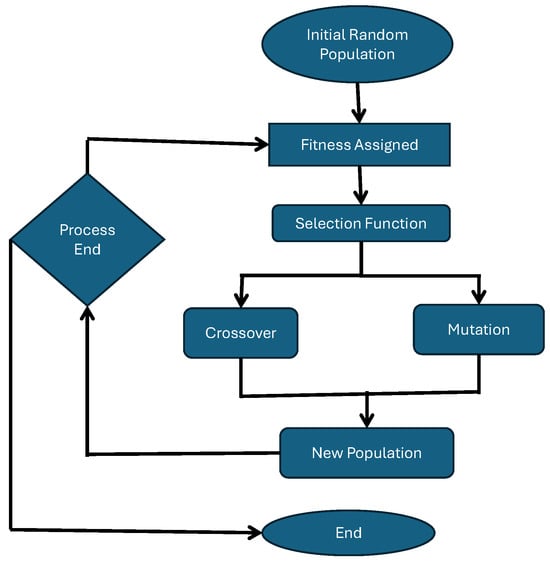
Figure 2.
Workflow of GP for model optimization.
2.4. XGBoost
XGBoost is a gradient-boosting framework that constructs a series of decision trees to minimize prediction errors. It uses a regularized objective function:
where : the loss function (e.g., squared error loss).
At each iteration, a new tree is fitted to the residuals of the previous trees:
The final prediction in XGBoost is a weighted sum of all the decision trees. XGBoost is particularly strong because it can handle missing data and incorporates regularization to prevent overfitting. Also, it uses parallel processing to optimize performance. In our study, key hyperparameters, such as the learning rate and tree depth, were carefully adjusted through cross-validation to enhance accuracy. Metrics like R2 and RMSE were used to evaluate the model’s performance.
Figure 3 illustrates the workflow of XGBoost, an advanced machine learning algorithm based on the gradient boosting framework. The process begins with a dataset that is used to train an ensemble of decision trees , , …, , each represented by its unique parameters , , …, . The first tree ) generates initial predictions, and the residuals (the errors between the predicted and actual values) are calculated. These residuals are then passed to the next tree ), which aims to correct the previous errors. This iterative process continues, with each subsequent tree learning from the residuals of the previous model. The node splitting in each tree is optimized based on an objective function, which improves predictive accuracy. Finally, the outputs from all trees are combined through an additive process and result in a high-performing predictive model. This ensemble approach enhances accuracy, reduces overfitting, and ensures efficient computation.
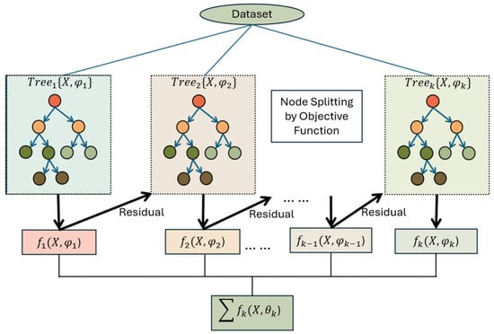
Figure 3.
Workflow of XGBoost algorithm for model development.
2.5. Hybrid (GP-XGBoost)
Combining GP and XGBoost creates a powerful hybrid methodology that integrates the interpretability of GP with the robust predictive capabilities of XGBoost. This combination is particularly valuable for solving complex problems where understanding the underlying relationships is as important as achieving high predictive accuracy. Below is a comprehensive outline of how these methods can be combined. In this research, method 2 was employed as it showed better performance in prediction.
Method 1. Sequential Hybrid Approach
In this approach, GP is used as a preprocessing step to create features or refine the input data for XGBoost, which then focuses on predictive modeling.
Step 1: Feature Engineering with GP
- 1.
- Symbolic Regression: GP is employed to explore relationships between input variables (e.g., the LL, the PI, and e0) and the target variable (Cc). The output is symbolic equations that describe the following relationships:
- 2.
- Feature Transformation: The symbolic equations are converted into new features, such as the following:
- 3.
- Feature Selection: The symbolic features are evaluated based on their importance and correlation with the target variable, and only the most relevant features are retained for the next step.
Step 2: Predictive Modeling with XGBoost
- 1.
- Dataset Augmentation: The refined features from GP are added to the original dataset, enriching the input space for XGBoost.
- 2.
- Training XGBoost: XGBoost is trained on the augmented dataset. The combination of raw and GP-derived features allows XGBoost to capture complex patterns and residual errors that are not fully explained by GP.
- 3.
- Evaluation: The performance of the model is assessed using metrics such as the MSE and R2.
By using GP’s symbolic equations, this approach improves XGBoost’s ability to generalize complex nonlinear relationships.
Method 2. Integrated Hybrid Approach
This approach iteratively combines GP and XGBoost, with feedback loops allowing both methods to influence each other.
Step 1: Initial Training with XGBoost
- 1.
- XGBoost is trained in the raw features to establish a baseline model.
- 2.
- The feature importance from XGBoost is extracted to identify which features contribute most to the predictions.
Step 2: Feedback to GP for Feature Discovery
- 1.
- GP uses the ranked features from XGBoost to focus on the most influential variables.
- 2.
- It generates symbolic relationships, such as Equations (11) and (12).
- 3.
- GP-derived features are added to the original dataset.
Step 3: Iterative Refinement
- 1.
- The new dataset, enriched by GP, is fed back into XGBoost for retraining.
- 2.
- XGBoost’s predictions and feature importances are analyzed, and further refinement of features is performed by GP.
- 3.
- This feedback loop continues until convergence or performance improvement stagnates.
Method 3. Parallel Hybrid Approach
In this approach, GP and XGBoost work independently, and their outputs are combined for the final prediction.
Step 1: Independent Training
- 1.
- GP is trained independently to create symbolic models for predicting Cc, generating outputs (CcGP).
- 2.
- XGBoost is trained independently on the same dataset to produce output (CcXGBoost).
Step 2: Weighted Combination of Outputs
- 1.
- The predictions from both models are combined using a weighted averaging approach:
- 2.
- Alternatively, a stacking ensemble can be used, where the outputs of GP and XGBoost serve as inputs to a meta-model that learns how to combine them optimally.
Step 3: Final Model Evaluation
The combined predictions are evaluated using standard performance metrics, ensuring that the complementary strengths of GP (interpretability) and XGBoost (accuracy) are fully utilized.
The hybrid GP-XGBoost approach combines the best features of two powerful methods and can offer distinct advantages. First, it improves model interpretability by using symbolic equations from GP which clearly show the relationships between input variables and the target. This is especially useful in geotechnical engineering where understanding soil behavior is key to making informed decisions. Second, the hybrid model boosts predictive accuracy by using XGBoost’s ability to handle complex, nonlinear patterns and residual errors. GP-derived features enhance the dataset and allow XGBoost to work with a richer, more meaningful input space. This often leads to better generalization and reduced overfitting. The method is also highly adaptable and makes it suitable for various datasets and applications where both precision and clarity are important.
The GP-XGBoost model is particularly effective for problems that involve complex nonlinear relationships and require both high accuracy and easy interpretation. GP’s symbolic equations help engineers understand the key factors driving these properties, while XGBoost ensures dependable predictions. Beyond geotechnics, the hybrid model is valuable in areas like environmental science where interactions between soil, water, and plants are critical. By combining symbolic reasoning with advanced machine learning, this hybrid approach bridges the gap between explainable and high-performance predictive models.
3. Results
3.1. Multiple Linear Regression (MLR) Predictions
The results from the MLR model show its limitations in predicting Cc, especially for the testing database. Figure 4 shows that the training data aligns reasonably well with the 1:1 reference line and indicates a decent fit for the known data. Many points fall outside of the ±10% boundaries and show that MLR struggles to generalize new data. This is because MLR relies on linear relationships. This linear approach is not enough to capture the complex, nonlinear interactions often seen in soil compressibility behavior.
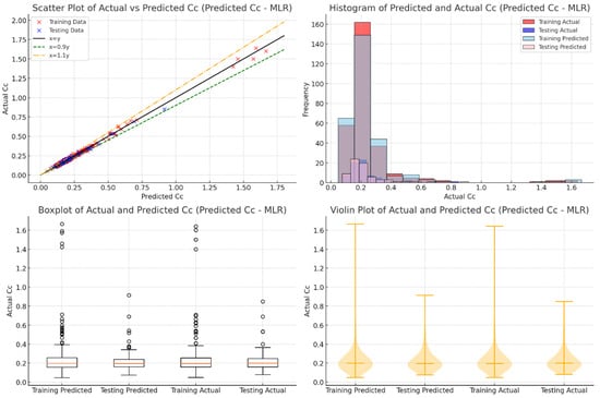
Figure 4.
Evaluation of actual vs. predicted Cc using MLR through various visualizations.
The boxplots and violin plots in Figure 4 further illustrate MLR’s shortcomings. The boxplots show wider interquartile ranges and more outliers in both the training and testing predictions compared to the actual values, and thus indicate less precision. The violin plots reveal broader and misaligned distributions for predicted values, especially in the testing dataset. This reflects MLR’s inability to handle the variability and complexity of real data. These results show the need for more advanced methods, such as machine learning models like XGBoost or GP, which are better suited to capture nonlinear relationships and improve prediction accuracy in complex geotechnical datasets.
Table 5 shows the performance of the MLR method in predicting Cc values for both training and testing databases. The model performs well and achieved an R2 of 0.879 for training and 0.843 for testing and indicated strong predictive accuracy and good generalization to new data.
Table 5.
The performance of the MLR method to predict Cc for training and testing databases.
The error metrics further support these results. The MAE values are 0.054 for training and 0.059 for testing, while the MSE values are 0.006 and 0.008, respectively. These low error rates highlight the MLR method’s ability to provide reliable predictions.
3.2. Genetic Programming (GP) Predictions
Figure 5 highlights how well the GP model predicts Cc values and shows a strong match between the predicted and actual results. In the scatter plot, most data points from both the training and testing datasets align closely with the 1:1 reference line. This approach reflects excellent accuracy. Many points also fall within the ±10% deviation bands and show that the model can generalize well with new data. However, the testing database shows slightly more scatter than the training data. This point shows that the model could be improved for more complex or extreme cases.

Figure 5.
Evaluation of actual vs. predicted Cc using GP through various visualizations.
The histogram, boxplot, and violin plot in Figure 5 provide more evidence of the GP model’s reliability. The histogram shows that the predicted values closely match the actual data distribution, especially for lower Cc values. The boxplots reveal very little difference between the median and interquartile ranges of the actual and predicted values, with only a few outliers. The violin plots show that the predicted data have a similar shape and spread to the actual values, further confirming the model’s consistency. These results show that the GP model captures nonlinear relationships well, and its symbolic regression makes it easy to interpret. This combination of accuracy and interpretability makes the GP model a powerful tool for predicting soil compressibility.
The following equation shows the GP proposed equation. Also, Table 6 represents parameters and constants:
Y = (r12 + (x1 − x2)2 × 4 × r1)2 × (x3 − r32 × x1 + (r2 + x3) × (x3 + x1) − x44 + (x22 − x32) × (2 × x1 − r3 − x4) × ((x1 − r1) × (2 × x2) − (3 × x3 + r1)))
Table 6.
Variables and parameters in GP proposed equation.
Table 7 presents the performance metrics of the GP method in predicting the Cc for the training and testing datasets. The GP method demonstrates strong predictive performance, with a high R2 value of 0.934 for the training database, indicating an excellent fit to the data. For the testing database, the R2 value is 0.827, reflecting good generalization capabilities. Additionally, the low mean absolute error (MAE) values of 0.039 and 0.040, along with mean squared error (MSE) values of 0.003 for both datasets, highlight the GP method’s ability to capture complex relationships and provide accurate predictions for both training and testing datasets.
Table 7.
The performance of the GP method to predict Cc for training and testing databases.
The GP model was optimized using an evolutionary strategy that balances accuracy and interpretability. The best configuration was obtained by tournament selection and elitism, ensuring diversity while avoiding premature convergence. Table 8 shows optimized hyperparameters for GP.
Table 8.
Optimized hyperparameters for GP.
3.3. XGBoost Predictions
Figure 6 illustrates the strong performance of the XGBoost model in predicting Cc values. Most data points for both the training and testing sets are closely aligned with the 1:1 line, showing a high correlation between the predicted and actual values. The minimal scatter of points indicates excellent accuracy and consistency in the model’s predictions. The addition of ±10% deviation lines further highlights that the majority of predictions fall within an acceptable error range, demonstrating XGBoost’s ability to capture complex and nonlinear patterns in the data. A few points outside these lines suggest areas where fine-tuning hyperparameters or adding features could enhance performance.
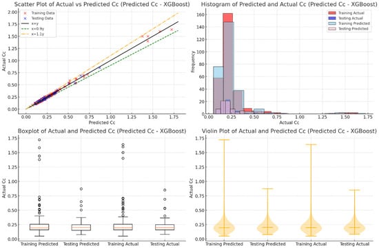
Figure 6.
Evaluation of actual vs. predicted Cc using XGBoost through various visualizations.
The histogram, boxplot, and violin plot in Figure 6 add more evidence of XGBoost’s reliability. The histogram shows a close match between the distributions of predicted and actual Cc values for both the training and testing datasets, suggesting strong generalization to unseen data. The boxplots reveal similar median values and interquartile ranges for the predicted and actual results, with only a few outliers. The violin plots provide a deeper look at data density, showing consistent shapes and patterns between actual and predicted values. These results confirm that XGBoost not only delivers accurate predictions but also maintains robust and consistent performance, making it a dependable choice for geotechnical applications.
Table 9 highlights how well the XGBoost model predicts Cc values for both training and testing datasets. The model performs great, with an R2 of 0.939 for the training set and an impressive 0.916 for the testing set. This shows that it not only makes accurate predictions but also generalizes well to new data.
Table 9.
The performance of XGBoost method to predict Cc for training and testing databases.
The error values add to this confidence. The MAE is 0.038 for the training set and 0.028 for the testing set, while the MSE is 0.002 and 0.001, respectively. These low error rates demonstrate the model’s precision and reliability. Overall, XGBoost stands out as a highly effective and consistent tool for geotechnical predictions.
To achieve the best predictive performance, Bayesian Optimization (TPE) was used for hyperparameter tuning. A 5-fold cross-validation approach was applied, and the best parameters were selected based on the lowest MSE. The optimized parameters for the XGBoost model are presented in Table 10.
Table 10.
Optimized hyperparameters for XGBoost.
3.4. Hybrid (GP-XGBoost) Predictions
Figure 7 shows the scatter plot that compares actual and predicted Cc values for the GP-XGBoost model. This figure highlights the strong predictive performance of this hybrid method. Most points from both the training and testing datasets align closely with the 1:1 reference line. This performance shows a high level of agreement between predictions and actual values. The points are tightly distributed within ±10% deviation lines and confirm the model’s accuracy and consistency. This demonstrates the hybrid model’s ability to effectively handle nonlinear relationships in the data and make it a reliable choice for predicting Cc. A few slight deviations suggest areas for potential improvement in feature representation or model assumptions.
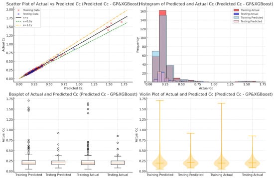
Figure 7.
Evaluation of actual vs. predicted Cc using hybrid GP-XGBoost model through various visualizations.
The histogram, boxplot, and violin plot in Figure 7 provide additional insights into the model’s performance. The histogram shows that predicted values closely follow the actual data distribution and peak around the mean Cc. The boxplot reveals minimal differences between median values and tightly grouped interquartile ranges and it further confirms the model’s accuracy. The violin plots give a more detailed view of data distribution. They show consistent density and effectively address outliers. Together, these visualizations emphasize the GP-XGBoost model’s robustness, precision, and reliability and make it a strong tool for geotechnical predictions that require high confidence.
Table 11 shows how well the Hybrid GP-XGBoost model predicts Cc values for both training and testing datasets. The model delivers excellent results, with an R2 of 0.966 for the training set and 0.927 for the testing set. The results represent high accuracy and strong generalization. The low mean absolute error (MAE) values of 0.030 for the training set and 0.028 for the testing set, along with a minimal mean squared error (MSE) of 0.001 for both datasets, demonstrate its precision in handling complex relationships.
Table 11.
The performance of the hybrid GP-XGBoost method to predict Cc for training and testing databases.
This performance highlights the model’s ability to outperform individual methods, proving its reliability and robustness. By effectively capturing the complexities of the data, the Hybrid GP-XGBoost model stands out as a highly dependable approach for accurate predictions.
The following equation shows the GP-XGBoost proposed equation. Also, Table 12 represents parameters and constants:
Y = ((R1 + R2) × X3 × R1 + (((4 × X3 − R3) × (X3 − X2 + X1 − X4))2)) + (((R1 + R2 × X4) × (R1 + R2) × (X4 × R1) × X2 × R1) − ((X3 − X4) × ((X3 − X2 + R3 − X4) − ((X2 − X3) × (2 × X3 − X1)))))
Table 12.
Variables and parameters in GP-XGBoost proposed equation.
For the GP-XGBoost hybrid model, the best approach involved iterative refinement:
Feature Selection: Only the top four most important GP-derived features were used in XGBoost.
A stacking ensemble approach was used, where a meta-model determined the optimal contribution of GP and XGBoost outputs. A grid search was performed to find the best weight combination. Table 13 shows optimized hyperparameters for GP-XGBoost.
Table 13.
Optimized hyperparameters for GP-XGBoost.
4. Discussion
4.1. Residual Analysis and Error Distribution for Model Performance Evaluation
Figure 8 compares the results of different models using several graphs. Residual plots show the differences between the actual and predicted values, which help assess accuracy and bias. Ideally, the residuals should be evenly spread around zero, indicating no bias in the model’s predictions. Models like GP and XGBoost perform well, with residuals mostly close to zero, showing good accuracy. On the other hand, scattered residuals highlighted areas where predictions were less accurate. These graphs also reveal the range of errors, with narrower distributions around zero indicating better performance, as seen in GP and XGBoost. Wider or skewed distributions suggest models with lower accuracy or potential biases.
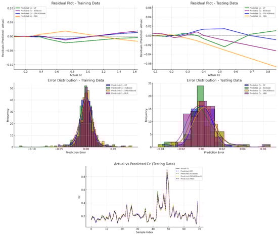
Figure 8.
Residual and error distribution analysis of Cc predictions across GP, XGBoost, GP-XGBoost, and MLR models.
The scatter matrix in Figure 8 compares actual Cc values with the predicted ones for each model. Points closer to the diagonal line indicate more accurate predictions. GP and XGBoost models show tight clustering along the diagonal direction, reflecting higher accuracy, while scattered points in other models reveal more errors. This visualization is useful for identifying how well each model generalizes to new data and whether there are any consistent issues. It offers a clear view of the models’ strengths and weaknesses, making it easier to understand their overall performance.
4.2. Feature Importance
Feature importance is a key concept in machine learning that helps explain which factors have the biggest impact on a model’s predictions. It shows how much each variable contributes to the model’s performance and helps researchers understand the relationships within the data. The method for calculating feature importance depends on the model. For example, in tree-based models like XGBoost, it can be measured by how much a feature reduces errors or how often it is used in decision splits. In GP models, importance is assessed by analyzing symbolic equations to see how strongly a feature influences the output. For hybrid models like GP-XGBoost, these methods are combined with techniques like permutation importance or SHAP values, which quantify how much each feature contributes to the predictions. These tools make it easier to rank features, interpret results, and improve the model.
The feature importance results in Figure 9 reveal how different soil properties—such as the initial void ratio (e0), the liquid limit (LL), the plasticity index (PI), and the water content (w)—affect the prediction of the compression index (Cc). The initial void ratio (e0) stands out as the most important factor, especially in the GP-XGBoost hybrid model, where it has the highest importance score of 0.55. This highlights its critical role in soil compressibility, as it reflects the soil’s structure and potential for volume change. The LL and the PI also contribute significantly, particularly in GP-XGBoost and GP models, with importance scores of 0.240 and 0.220. These properties are linked to soil composition and plasticity, making them reliable indicators of compressibility. Interestingly, water content (w) is moderately important in the hybrid model, with a score of 0.270, showing its effect on soil behavior. MLR assigns less importance to all features, especially the LL and the w, due to its limited ability to handle complex relationships. These results demonstrate how GP-XGBoost combines the strengths of both GP and XGBoost to give a detailed understanding of soil behavior through feature analysis.
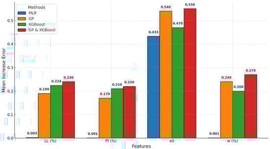
Figure 9.
Feature importance comparison for predicting Cc across MLR, GP, XGBoost, and GP-XGBoost models.
It is important to note that the dependency between the liquid limit (LL) and the plasticity index (PI) may have influenced the feature importance rankings. Since the PI is derived from the LL and the PL, this relationship introduces collinearity, potentially inflating the importance of these features in the predictive models. Although the GP-XGBoost model is robust against multicollinearity, this dependency could affect the interpretability of the results, and it is acknowledged as a limitation of this study.
Feature importance ranking aligns with fundamental geotechnical principles and reflects the critical role of soil composition and structure in compressibility behavior.
The LL and the PI are indicators of a soil’s clay mineral content and plasticity, which directly affect compressibility. Higher LL values are typically associated with fine-grained soils rich in montmorillonite or kaolinite, which have a greater capacity to absorb water and undergo volume changes under load. The PI reflects the soil’s ability to deform plastically, and a higher PI usually correlates with the greater rearrangement of particles during consolidation, resulting in higher Cc values. The strong feature importance of LL and PI in the model suggests that mineralogical composition and interparticle bonding are key mechanisms driving compressibility.
The initial void ratio is a fundamental measure of the porosity and packing density of soil particles. Soils with a high e0 have more interparticle voids that make them more susceptible to settlement when subjected to load. The model’s emphasis on e0 highlights the significance of soil structure, particularly the arrangement of particles and pore spaces, in controlling the magnitude of primary consolidation.
The natural moisture content influences the pore water pressure, effective stress, and the ease with which particles can rearrange under loading conditions. Soils with higher moisture content tend to have weaker interparticle forces and facilitate greater compression.
The feature importance analysis suggests that the compression index (Cc) is governed by a combination of the following features:
- -
- Mineralogical properties (the LL, the PI, and specific gravity) affect plasticity and particle interaction.
- -
- Structural characteristics (the initial void ratio) influence particle arrangement and porosity.
- -
- Hydrological conditions (the natural moisture content) impact pore water dynamics and effective stress.
These findings align with the classical consolidation theory, where Cc is a function of both soil composition and initial structural conditions. Machine learning models not only confirm these geotechnical principles but also provide quantitative evidence of the relative importance of each factor.
4.3. Comparison with the Literature
Figure 10 compares the Cc values predicted by different models with the actual observed values. The models include GP-XGBoost, Terzaghi and Peck [1], Azzouz et al. [8], Koppula [9], and Yoshinaka and Osada [11]. The GP-XGBoost model closely matches actual values, especially for lower Cc ranges. In contrast, the empirical models show larger deviations. Terzaghi and Peck [1] often overestimate Cc, while Azzouz et al. [8] significantly underestimates it. Koppula [9] and Yoshinaka and Osada [11] provide more consistent results but lack the precision of GP-XGBoost.
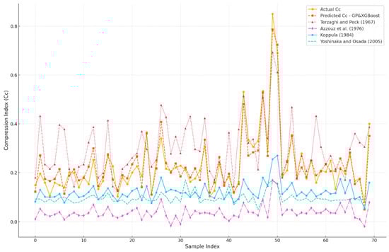
Figure 10.
Scatter matrix plot of actual and predicted Cc for testing data using different models [1,8,9,11].
These results highlight the strength of machine learning models like GP-XGBoost in capturing complex relationships in the data. They outperform empirical models, which are limited by their assumptions and simplified formulas. The graph also shows the variability in soil behavior and the difficulty that empirical methods have in generalizing across different conditions. While traditional models are useful for initial estimates, GP-XGBoost offers higher reliability and accuracy. This makes it a valuable tool for geotechnical engineering and emphasizes the importance of modern, data-driven techniques.
The results in Table 14 show that the GP-XGBoost hybrid model performs better than empirical models in predicting Cc. The GP-XGBoost model achieved a high R2 of 0.927 and a low MSE of 0.027. This shows it has strong accuracy and minimal error. In comparison, empirical models had much lower R2 values. Terzaghi and Peck [1] had the highest R2 at 0.149, while others had R2 < 0.1 values that show a poor fit or overestimation.
Table 14.
Performance comparison of GP and XGBoost with empirical models for predicting Cc.
MAE values for the empirical models were also much higher. They ranged from 0.090 for Terzaghi and Peck [1] to 0.189 for Azzouz et al. [8]. These results show that GP-XGBoost is effective at capturing complex patterns in the data. Traditional empirical models fail to represent these relationships accurately.
4.4. Limitations and Future Work
The hybrid GP-XGBoost approach is effective but faces challenges in computation and practical use. GP’s symbolic regression can create complex equations that are hard to use in real-time. XGBoost also needs significant computing power for its iterative training on enhanced datasets. This may not be feasible for small engineering firms or in developing areas. To address this, future studies can focus on simplifying GP-generated equations or applying dimensionality reduction techniques. Cloud-based or easy-to-use software can make the models more accessible.
Overfitting is another issue in machine learning. It can produce good results on training data but poor results on new data. This study used normalization and cross-validation, but more work is needed. Testing with data from different regions can help. Techniques like dropout regularization and ensemble methods can reduce overfitting. Tools like SHAP values can show how features affect predictions. This will build trust and support the wider use of the models.
One limitation of this study is the inherent dependency between some input parameters, particularly the LL and the PI. Since the PI is calculated directly from the LL and the PL, this introduces collinearity, which may affect the stability and interpretability of feature importance in the models. Although the hybrid GP-XGBoost model is capable of handling such dependencies, future research could benefit from employing dimensionality reduction techniques or regularization methods to mitigate these effects and enhance model robustness.
Building upon the findings and acknowledging the limitations of this study, several directions for future research are proposed to enhance the robustness, generalizability, and interpretability of the predictive models for the compression index (Cc):
- -
- Future studies should explore dimensionality reduction techniques, such as Principal Component Analysis (PCA), to transform correlated features into uncorrelated components. Alternatively, regularization methods like LASSO regression can be applied to reduce the influence of redundant variables.
- -
- The current dataset, while comprehensive, lacks geographical and geological diversity. Future work should incorporate larger, multi-regional datasets that cover a wider range of soil types, climatic conditions, and geotechnical properties.
- -
- To ensure the generalizability of the proposed model, future research should involve external validation using independent datasets from different projects or geographical locations.
- -
- Although the GP-XGBoost hybrid model offers high accuracy, its complex symbolic equations can hinder interpretability. Future studies could focus on developing simplified symbolic models by incorporating genetic simplification algorithms or rule-based pruning techniques to generate more concise, physically interpretable expressions that align with geotechnical principles.
- -
- While the hybrid GP-XGBoost model demonstrated strong performance, future research could explore advanced ensemble techniques such as stacking, blending, or meta-learning frameworks to further enhance predictive accuracy. Additionally, integrating deep learning models like Recurrent Neural Networks (RNNs) or Attention Mechanisms could improve the capture of complex temporal and spatial patterns in geotechnical data.
4.5. Statistical Significance Analysis and Model Comparison
To ensure the reliability of the predictive models, 30 independent runs were conducted for each model (MLR, GP, XGBoost, and GP-XGBoost) with different random seeds to account for variability in data splitting and model initialization. The performance metrics—R2, MSE, and MAE—were calculated for each run. This approach allows for a comprehensive assessment of each model’s performance. The mean and standard deviation of these metrics were computed to quantify the models’ central tendency and variability, as shown in Table 15.
Table 15.
Statistical summary of model performance (30 runs).
These results indicate that the hybrid GP-XGBoost model consistently outperformed other models with the highest mean R2 and the lowest MSE and MAE.
4.5.1. One-Way ANOVA Test
To determine if the observed differences in model performance were statistically significant, a one-way Analysis of Variance (ANOVA) test was applied. ANOVA is a strong statistical method that is used to compare the means of multiple groups (in this case, the performance metrics of different models) and assess whether at least one model performs differently from the others. The null hypothesis (H0) assumes no significant difference among the models, while the alternative hypothesis (H1) suggests that at least one model shows superior performance. The F-statistic and corresponding p-values were calculated for each performance metric (R2, MSE, and MAE). A p-value less than 0.05 indicates that the null hypothesis can be confidently rejected and confirms that significant performance differences exist between models (refer to Table 16).
Table 16.
ANOVA results.
4.5.2. Post-Hoc Tukey’s HSD Test
Following the ANOVA test, which identified significant differences among models, we conducted a Tukey’s Honestly Significant Difference (HSD) test as a post-hoc analysis. Tukey’s HSD test is designed to determine which specific model pairs exhibit statistically significant differences. This method compares all possible pairs of models and adjusts for multiple comparisons to control the family-wise error rate. The test provides p-values that indicate the likelihood that performance differences between two models occurred by chance. p-values less than 0.05 suggest a statistically significant difference between model performances. This analysis offers a detailed understanding of how each model compares against others, as summarized in Table 17.
Table 17.
Tukey’s HSD test results (p-values).
4.5.3. Model Validation Techniques
The model validation techniques employed in this study were designed to rigorously assess the predictive performance and reliability of the proposed models. Initially, the dataset was randomly split into 80% training and 20% testing subsets to evaluate model generalization, with random seeds used to ensure reproducibility across multiple runs. To further reduce the risk of overfitting and obtain robust performance metrics, a 5-fold cross-validation approach was implemented, where the dataset was divided into five subsets, using four for training and one for validation in a rotating manner. To enhance the reliability of the results, the entire modelling process was repeated 30 times with different random splits, and the mean and standard deviation of key performance metrics (R2, MSE, and MAE) were calculated to assess model stability. Finally, statistical significance tests, including ANOVA and Tukey’s HSD, were conducted to verify that performance differences between models were statistically significant, adding an extra layer of validation to this study’s findings.
5. Conclusions
This study proposed a hybrid GP-XGBoost model for predicting the compression index (Cc) of clayey soils, integrating the symbolic regression capabilities of Genetic Programming (GP) with the robust predictive power of Extreme Gradient Boosting (XGBoost). The model demonstrated superior performance compared to traditional empirical methods and standalone machine learning models, achieving an R2 of 0.927 with significantly reduced prediction errors. The feature importance analysis highlighted key geotechnical parameters—such as the liquid limit (LL), the plasticity index (PI), the initial void ratio (e0), and the natural moisture content (wn)—as critical factors influencing soil compressibility, aligning with established soil mechanics principles.
Despite the promising results, this study acknowledges several limitations, including parameter dependencies (e.g., the LL and the PI), limited dataset diversity, and potential overfitting risks. To address these challenges, future research should incorporate dimensionality reduction techniques, external validation with independent datasets, and simplified symbolic models for enhanced interpretability. Additionally, expanding the dataset to include diverse soil types and environmental conditions will improve the model’s generalizability in real-world applications.
The findings of this research offer valuable insights for geotechnical engineers involved in foundation design, settlement analysis, and infrastructure planning, providing a data-driven approach to complement traditional soil mechanics theories. By advancing predictive modeling techniques and addressing the identified limitations, future studies can further improve the accuracy, reliability, and practical applicability of machine learning models in geotechnical engineering.
Author Contributions
Conceptualization, A.B. and K.K.; methodology, A.B.; software, K.K.; validation, A.B., H.A.-N. and Y.L.; formal analysis, A.B., H.A.-N. and Y.L.; investigation, K.K.; resources, K.K.; data curation, K.K.; writing—original draft preparation, A.B.; writing—review and editing, H.A.-N. and Y.L.; visualization, K.K.; supervision, H.A.-N.; project administration, A.B. All authors have read and agreed to the published version of the manuscript.
Funding
This research received no external funding.
Institutional Review Board Statement
Not applicable.
Informed Consent Statement
Not applicable.
Data Availability Statement
The original contributions presented in this study are included in the article. Further inquiries can be directed to the corresponding authors.
Conflicts of Interest
The authors declare no conflicts of interest.
Abbreviations
The following abbreviations are used in this manuscript:
| Cc | Compression Index |
| MLR | Multiple Linear Regression |
| GP | Genetic Programming |
| XGBoost | eXtreme Gradient Boosting |
| MAE | Mean Absolute Error |
| MSE | Mean Squared Error |
| R2 | Coefficient of Determination |
| ML | Machine Learning |
| LL | Liquid Limit |
| PI | Plasticity Index |
| e0 | Void Ratio |
| w | Water Content |
Appendix A
Table A1.
Used database in this study.
Table A1.
Used database in this study.
| No. | LL (%) | PI (%) | e0 | w (%) | Cc |
|---|---|---|---|---|---|
| 1 | 56 | 36 | 0.498 | 20.2 | 0.169 |
| 2 | 30 | 10 | 0.718 | 29.7 | 0.11 |
| 3 | 35 | 15 | 0.883 | 36.6 | 0.246 |
| 4 | 29 | 7 | 0.753 | 32.1 | 0.213 |
| 5 | 40 | 22 | 0.695 | 24.4 | 0.123 |
| 6 | 39 | 19 | 0.77 | 29 | 0.279 |
| 7 | 48 | 25 | 0.724 | 25.6 | 0.163 |
| 8 | 33 | 10 | 0.632 | 22.6 | 0.116 |
| 9 | 30 | 8 | 0.546 | 20.3 | 0.149 |
| 10 | 40 | 21 | 0.585 | 23.7 | 0.22 |
| 11 | 52 | 28 | 0.731 | 29.4 | 0.22 |
| 12 | 54 | 31 | 0.755 | 29.8 | 0.149 |
| 13 | 58 | 36 | 0.867 | 34 | 0.196 |
| 14 | 50 | 29 | 0.74 | 31.2 | 0.259 |
| 15 | 49 | 28 | 0.97 | 36.5 | 0.29 |
| 16 | 36 | 17 | 0.676 | 26.5 | 0.159 |
| 17 | 47 | 29 | 0.826 | 31.4 | 0.179 |
| 18 | 38 | 17 | 0.529 | 19.4 | 0.11 |
| 19 | 45 | 22 | 0.809 | 27.1 | 0.22 |
| 20 | 46 | 25 | 0.775 | 30.3 | 0.173 |
| 21 | 47 | 26 | 0.717 | 28.9 | 0.246 |
| 22 | 29 | 11 | 0.71 | 24.7 | 0.19 |
| 23 | 47 | 24 | 0.915 | 37.5 | 0.29 |
| 24 | 29 | 8 | 0.717 | 20.5 | 0.146 |
| 25 | 34 | 12 | 0.668 | 24.1 | 0.106 |
| 26 | 36 | 17 | 0.676 | 26.5 | 0.159 |
| 27 | 35 | 13 | 0.825 | 30.8 | 0.2 |
| 28 | 31 | 12 | 0.621 | 23.9 | 0.156 |
| 29 | 43 | 20 | 0.732 | 26.9 | 0.163 |
| 30 | 30 | 8 | 0.605 | 23.9 | 0.133 |
| 31 | 54 | 31 | 0.755 | 29.8 | 0.149 |
| 32 | 25 | 5 | 0.869 | 30.8 | 0.2 |
| 33 | 53 | 28 | 0.583 | 22.4 | 0.169 |
| 34 | 52 | 28 | 0.517 | 19.5 | 0.14 |
| 35 | 45 | 22 | 0.652 | 27.1 | 0.18 |
| 36 | 52 | 28 | 0.806 | 28.9 | 0.28 |
| 37 | 25 | 5 | 1.222 | 48.7 | 0.41 |
| 38 | 34 | 12 | 0.675 | 25.2 | 0.229 |
| 39 | 33 | 10 | 0.768 | 31.4 | 0.252 |
| 40 | 36 | 14 | 0.753 | 29.7 | 0.2 |
| 41 | 53 | 29 | 0.98 | 39 | 0.26 |
| 42 | 34 | 13 | 0.734 | 25.3 | 0.2 |
| 43 | 26 | 8 | 0.824 | 28.9 | 0.199 |
| 44 | 27 | 9 | 0.63 | 20 | 0.193 |
| 45 | 39 | 19 | 0.667 | 26.4 | 0.279 |
| 46 | 33 | 13 | 0.789 | 33.6 | 0.279 |
| 47 | 35 | 16 | 0.663 | 25.2 | 0.14 |
| 48 | 27 | 8 | 0.675 | 24.1 | 0.126 |
| 49 | 31 | 11 | 0.736 | 25.9 | 0.21 |
| 50 | 35 | 14 | 0.675 | 25.3 | 0.13 |
| 51 | 47 | 26 | 0.785 | 29.8 | 0.173 |
| 52 | 27 | 5 | 0.519 | 11.1 | 0.126 |
| 53 | 40 | 18 | 0.588 | 25.2 | 0.16 |
| 54 | 54 | 30 | 0.776 | 31.2 | 0.183 |
| 55 | 29 | 8 | 0.663 | 26.7 | 0.12 |
| 56 | 29 | 7 | 0.637 | 22.7 | 0.183 |
| 57 | 44 | 24 | 0.629 | 27 | 0.166 |
| 58 | 27 | 8 | 0.661 | 25.3 | 0.156 |
| 59 | 56 | 34 | 0.612 | 22.6 | 0.15 |
| 60 | 36 | 15 | 0.697 | 25 | 0.183 |
| 61 | 31 | 11 | 0.831 | 29.8 | 0.176 |
| 62 | 43 | 22 | 0.798 | 29 | 0.209 |
| 63 | 33 | 14 | 0.69 | 24.9 | 0.13 |
| 64 | 53 | 35 | 0.642 | 23.1 | 0.169 |
| 65 | 46 | 22 | 0.801 | 28.6 | 0.153 |
| 66 | 53 | 27 | 0.97 | 39.8 | 0.252 |
| 67 | 34 | 15 | 0.761 | 23.7 | 0.189 |
| 68 | 31 | 11 | 0.723 | 25.3 | 0.169 |
| 69 | 58 | 35 | 0.807 | 27.3 | 0.229 |
| 70 | 37 | 18 | 0.802 | 27.3 | 0.179 |
| 71 | 36 | 14 | 0.777 | 27.4 | 0.229 |
| 72 | 42 | 22 | 0.658 | 21.7 | 0.22 |
| 73 | 31 | 11 | 0.769 | 27.2 | 0.176 |
| 74 | 37 | 16 | 0.776 | 31.8 | 0.166 |
| 75 | 34 | 12 | 0.824 | 28.1 | 0.269 |
| 76 | 34 | 14 | 0.573 | 22.1 | 0.123 |
| 77 | 27 | 6 | 0.643 | 22.4 | 0.189 |
| 78 | 43 | 21 | 0.643 | 22.1 | 0.203 |
| 79 | 32 | 10 | 0.644 | 27 | 0.196 |
| 80 | 35 | 13 | 0.652 | 23.2 | 0.206 |
| 81 | 39 | 20 | 0.653 | 28.5 | 0.186 |
| 82 | 26 | 8 | 0.824 | 28.9 | 0.199 |
| 83 | 30 | 8 | 0.605 | 23.9 | 0.133 |
| 84 | 29 | 9 | 0.777 | 28.4 | 0.14 |
| 85 | 43 | 20 | 0.732 | 26.9 | 0.163 |
| 86 | 39 | 17 | 0.73 | 25.8 | 0.196 |
| 87 | 29 | 11 | 0.658 | 25.1 | 0.149 |
| 88 | 37 | 16 | 0.738 | 25.1 | 0.203 |
| 89 | 31 | 14 | 0.619 | 26.4 | 0.14 |
| 90 | 30 | 15 | 0.746 | 26.2 | 0.183 |
| 91 | 60 | 30 | 0.733 | 26.3 | 0.196 |
| 92 | 30 | 10 | 0.602 | 22.6 | 0.13 |
| 93 | 31 | 7 | 0.738 | 27.5 | 0.173 |
| 94 | 30 | 10 | 0.874 | 31.1 | 0.209 |
| 95 | 33 | 12 | 0.703 | 28 | 0.103 |
| 96 | 43 | 19 | 0.828 | 29.8 | 0.186 |
| 97 | 32 | 10 | 0.718 | 25.7 | 0.166 |
| 98 | 31 | 11 | 0.635 | 23.1 | 0.146 |
| 99 | 56 | 28 | 0.909 | 36.9 | 0.27 |
| 100 | 34 | 15 | 0.739 | 27.5 | 0.146 |
| 101 | 37 | 15 | 0.761 | 29.6 | 0.173 |
| 102 | 42 | 20 | 0.716 | 26.9 | 0.216 |
| 103 | 37 | 17 | 0.723 | 26 | 0.21 |
| 104 | 44 | 22 | 0.667 | 26.7 | 0.123 |
| 105 | 26 | 6 | 0.704 | 24.8 | 0.226 |
| 106 | 24 | 4 | 0.558 | 22 | 0.103 |
| 107 | 34 | 13 | 0.745 | 24.7 | 0.18 |
| 108 | 37 | 15 | 0.873 | 27.6 | 0.329 |
| 109 | 39 | 17 | 0.993 | 41.1 | 0.259 |
| 110 | 60 | 36 | 1.008 | 49.2 | 0.249 |
| 111 | 51 | 27 | 0.854 | 34.8 | 0.249 |
| 112 | 36 | 19 | 0.678 | 27.2 | 0.153 |
| 113 | 33 | 14 | 0.677 | 27.2 | 0.17 |
| 114 | 39 | 17 | 0.837 | 31.9 | 0.2 |
| 115 | 44 | 24 | 0.965 | 37.8 | 0.229 |
| 116 | 62 | 44 | 1.014 | 38.4 | 0.326 |
| 117 | 41 | 20 | 0.909 | 35.3 | 0.226 |
| 118 | 37 | 17 | 0.721 | 28 | 0.163 |
| 119 | 37 | 17 | 0.734 | 28.3 | 0.159 |
| 120 | 39 | 19 | 0.761 | 24.5 | 0.183 |
| 121 | 38 | 17 | 0.563 | 21.8 | 0.103 |
| 122 | 33 | 16 | 0.894 | 34 | 0.329 |
| 123 | 47 | 27 | 0.736 | 29.8 | 0.25 |
| 124 | 45 | 22 | 0.537 | 11.5 | 0.13 |
| 125 | 52 | 28 | 0.615 | 17.6 | 0.21 |
| 126 | 46 | 23 | 0.611 | 18.5 | 0.173 |
| 127 | 51 | 25 | 0.586 | 19.2 | 0.186 |
| 128 | 30 | 10 | 0.782 | 32.2 | 0.159 |
| 129 | 35 | 13 | 0.841 | 35.3 | 0.256 |
| 130 | 43 | 22 | 0.964 | 31.1 | 0.365 |
| 131 | 49 | 29 | 0.805 | 32.1 | 0.233 |
| 132 | 79 | 45 | 1.587 | 57.4 | 0.628 |
| 133 | 35 | 15 | 0.507 | 23.5 | 0.11 |
| 134 | 37 | 10 | 0.928 | 40.9 | 0.31 |
| 135 | 49 | 28 | 0.797 | 32.8 | 0.309 |
| 136 | 51 | 32 | 0.829 | 32 | 0.31 |
| 137 | 38 | 17 | 0.79 | 30.5 | 0.249 |
| 138 | 42 | 20 | 0.755 | 30.3 | 0.193 |
| 139 | 41 | 22 | 0.816 | 31.4 | 0.266 |
| 140 | 39 | 19 | 0.725 | 28.5 | 0.183 |
| 141 | 63 | 34.15 | 1.2 | 47.1 | 0.34 |
| 142 | 46 | 24 | 0.847 | 33.6 | 0.296 |
| 143 | 34 | 13 | 0.675 | 22 | 0.216 |
| 144 | 57.5 | 33.2 | 0.806 | 25 | 0.216 |
| 145 | 56 | 33.4 | 0.704 | 22.8 | 0.141 |
| 146 | 58.2 | 29.4 | 0.571 | 20.8 | 0.143 |
| 147 | 57.2 | 28.5 | 0.821 | 22.6 | 0.246 |
| 148 | 51.9 | 21.7 | 0.656 | 21.8 | 0.179 |
| 149 | 45.6 | 22.6 | 0.747 | 12.4 | 0.188 |
| 150 | 40.5 | 20.9 | 0.663 | 16.7 | 0.188 |
| 151 | 40.9 | 23.2 | 0.872 | 11.2 | 0.206 |
| 152 | 50.2 | 23.5 | 0.671 | 19 | 0.194 |
| 153 | 47.6 | 25.6 | 0.612 | 17.2 | 0.158 |
| 154 | 50.4 | 26 | 0.782 | 24.3 | 0.176 |
| 155 | 48.7 | 24.1 | 0.844 | 24.9 | 0.221 |
| 156 | 40.2 | 18 | 0.644 | 17.7 | 0.15 |
| 157 | 44.6 | 15.5 | 0.714 | 18.6 | 0.198 |
| 158 | 34.8 | 14.7 | 0.52 | 21.9 | 0.135 |
| 159 | 44 | 24.3 | 0.56 | 17.7 | 0.176 |
| 160 | 49.1 | 30 | 0.511 | 16.2 | 0.123 |
| 161 | 41.1 | 22.1 | 0.78 | 13.3 | 0.228 |
| 162 | 49.8 | 18.7 | 0.968 | 33.3 | 0.241 |
| 163 | 52.3 | 11.7 | 0.786 | 37 | 0.211 |
| 164 | 42.7 | 9.2 | 0.745 | 27.6 | 0.158 |
| 165 | 61.4 | 19.8 | 0.938 | 31.2 | 0.199 |
| 166 | 50.9 | 17 | 1.06 | 29.2 | 0.236 |
| 167 | 57.8 | 32.9 | 0.669 | 22.4 | 0.163 |
| 168 | 42.9 | 8.4 | 0.797 | 31.3 | 0.176 |
| 169 | 31 | 10 | 1.232 | 46.4 | 0.465 |
| 170 | 29 | 10 | 0.77 | 27.2 | 0.183 |
| 171 | 48 | 25 | 0.756 | 29.9 | 0.163 |
| 172 | 68 | 42 | 0.884 | 38.5 | 0.322 |
| 173 | 42 | 24 | 0.657 | 28 | 0.209 |
| 174 | 40 | 17 | 0.931 | 39.3 | 0.209 |
| 175 | 32 | 8 | 0.979 | 39.4 | 0.266 |
| 176 | 27 | 6 | 0.817 | 28.9 | 0.176 |
| 177 | 57 | 35 | 1.031 | 28.9 | 0.306 |
| 178 | 26 | 8 | 0.676 | 20.1 | 0.113 |
| 179 | 46 | 25 | 0.647 | 23.8 | 0.123 |
| 180 | 33 | 12 | 0.703 | 28 | 0.103 |
| 181 | 45 | 26 | 0.808 | 34.5 | 0.319 |
| 182 | 30 | 11 | 0.681 | 25.2 | 0.163 |
| 183 | 44 | 25 | 0.816 | 34.2 | 0.239 |
| 184 | 32 | 11 | 0.703 | 28.8 | 0.206 |
| 185 | 29 | 9 | 0.643 | 25.5 | 0.126 |
| 186 | 52 | 31 | 1.132 | 45.7 | 0.379 |
| 187 | 37 | 14 | 0.928 | 35 | 0.233 |
| 188 | 34 | 14 | 0.676 | 24.6 | 0.226 |
| 189 | 64 | 31 | 1.647 | 64.1 | 0.53 |
| 190 | 33 | 15 | 0.786 | 31 | 0.193 |
| 191 | 56 | 35 | 0.569 | 25.2 | 0.146 |
| 192 | 44 | 21 | 0.476 | 14.5 | 0.126 |
| 193 | 28 | 7 | 0.598 | 22.6 | 0.173 |
| 194 | 28 | 7 | 0.619 | 22.8 | 0.153 |
| 195 | 50 | 27 | 0.771 | 33.1 | 0.176 |
| 196 | 46.5 | 18.7 | 1.243 | 10.9 | 0.317 |
| 197 | 50.5 | 14 | 0.796 | 17.8 | 0.183 |
| 198 | 48 | 24 | 0.84 | 50 | 0.3 |
| 199 | 25 | 7.5 | 0.5 | 20 | 0.2 |
| 200 | 42 | 22.6 | 0.604 | 22 | 0.136 |
| 201 | 63 | 50 | 0.817 | 30 | 0.133 |
| 202 | 45.9 | 21.1 | 0.577 | 21 | 0.152 |
| 203 | 44.1 | 22.9 | 0.706 | 29 | 0.173 |
| 204 | 61 | 32 | 0.754 | 26.5 | 0.17 |
| 205 | 39 | 19.1 | 0.537 | 25 | 0.121 |
| 206 | 26 | 10 | 0.525 | 25 | 0.117 |
| 207 | 51.9 | 28.1 | 0.612 | 23 | 0.162 |
| 208 | 22 | 5 | 0.671 | 24 | 0.121 |
| 209 | 43.8 | 19.14 | 0.703 | 29 | 0.316 |
| 210 | 36.2 | 24.15 | 0.722 | 30.3 | 0.325 |
| 211 | 38.2 | 17.25 | 0.669 | 28.4 | 0.248 |
| 212 | 67.1 | 39.95 | 1.149 | 42.4 | 0.531 |
| 213 | 41.2 | 12.08 | 0.875 | 29 | 0.279 |
| 214 | 38.5 | 14.43 | 0.76 | 29.8 | 0.26 |
| 215 | 45.9 | 27.48 | 0.895 | 30 | 0.334 |
| 216 | 47.5 | 23.18 | 0.743 | 29.1 | 0.306 |
| 217 | 44.7 | 20.92 | 0.817 | 35 | 0.307 |
| 218 | 33.7 | 22 | 0.641 | 25.2 | 0.33 |
| 219 | 48.6 | 17.66 | 0.946 | 33.9 | 0.347 |
| 220 | 66.6 | 44.29 | 1.196 | 45.9 | 0.534 |
| 221 | 106 | 67 | 2.86 | 120 | 1.5 |
| 222 | 48.7 | 20.2 | 0.886 | 13 | 0.231 |
| 223 | 80 | 30 | 1.86 | 57 | 1.5 |
| 224 | 46 | 22 | 1.1 | 38 | 0.35 |
| 225 | 50.2 | 14.1 | 0.859 | 23.2 | 0.248 |
| 226 | 46.9 | 10.5 | 0.813 | 16.6 | 0.199 |
| 227 | 46.5 | 11.5 | 0.9 | 17.9 | 0.241 |
| 228 | 47.9 | 11 | 0.966 | 22.5 | 0.287 |
| 229 | 46.5 | 9.8 | 0.94 | 19.8 | 0.253 |
| 230 | 52 | 30 | 1.2 | 44.2 | 0.511 |
| 231 | 46 | 22 | 0.96 | 35.6 | 0.289 |
| 232 | 51 | 31 | 1.2 | 44.4 | 0.535 |
| 233 | 47 | 24 | 1.26 | 47.2 | 0.465 |
| 234 | 66 | 40 | 1.22 | 45.1 | 0.382 |
| 235 | 45 | 25 | 0.95 | 34.6 | 0.368 |
| 236 | 125 | 82 | 2.9 | 108 | 1.64 |
| 237 | 70 | 31 | 1.8 | 64 | 0.7 |
| 238 | 87 | 47 | 1.7 | 73 | 0.85 |
| 239 | 76 | 38 | 1.8 | 67 | 0.66 |
| 240 | 78 | 42 | 1.8 | 68 | 0.69 |
| 241 | 62 | 31 | 1.4 | 55 | 0.54 |
| 242 | 100 | 44 | 1.4 | 53 | 0.71 |
| 243 | 25 | 8 | 0.7 | 25.4 | 0.13 |
| 244 | 63 | 34 | 1.4 | 48 | 0.59 |
| 245 | 63 | 34 | 1.4 | 48 | 0.62 |
| 246 | 116 | 69 | 2.9 | 131 | 1.4 |
| 247 | 135 | 81 | 3 | 124 | 1.6 |
| 248 | 50 | 26 | 1 | 35 | 0.2 |
| 249 | 40 | 18 | 1.045 | 40.7 | 0.259 |
| 250 | 44 | 26 | 0.761 | 32.1 | 0.199 |
| 251 | 32 | 12 | 0.665 | 21.6 | 0.166 |
| 252 | 30 | 11 | 0.752 | 26.1 | 0.183 |
| 253 | 28 | 9 | 0.73 | 19.5 | 0.113 |
| 254 | 40 | 19 | 0.715 | 19 | 0.219 |
| 255 | 34 | 15 | 0.613 | 18.4 | 0.153 |
| 256 | 55 | 28 | 1.322 | 49.6 | 0.409 |
| 257 | 58 | 35 | 1.059 | 39 | 0.385 |
| 258 | 34 | 14 | 0.871 | 31.2 | 0.176 |
| 259 | 56 | 34 | 0.983 | 36.1 | 0.306 |
| 260 | 37 | 15 | 0.88 | 33 | 0.209 |
| 261 | 62 | 36 | 1.054 | 32.7 | 0.355 |
| 262 | 62 | 36 | 0.806 | 34.4 | 0.312 |
| 263 | 40 | 21 | 0.926 | 30.9 | 0.379 |
| 264 | 55 | 30 | 0.921 | 37.4 | 0.246 |
| 265 | 41 | 22 | 0.804 | 31.4 | 0.229 |
| 266 | 39 | 20 | 0.748 | 29 | 0.233 |
| 267 | 48 | 25 | 0.724 | 25.6 | 0.163 |
| 268 | 39 | 21 | 0.647 | 25.3 | 0.259 |
| 269 | 30 | 9 | 0.702 | 25.3 | 0.189 |
| 270 | 39 | 21 | 0.647 | 25.3 | 0.259 |
| 271 | 44 | 23 | 0.815 | 35.3 | 0.183 |
| 272 | 34 | 14 | 0.676 | 24.6 | 0.225 |
| 273 | 40 | 19 | 0.8 | 29 | 0.279 |
| 274 | 34 | 12 | 0.692 | 25.8 | 0.173 |
| 275 | 32 | 11 | 0.699 | 20.4 | 0.173 |
| 276 | 33 | 10 | 0.707 | 27.8 | 0.176 |
| 277 | 24 | 4 | 0.695 | 26.3 | 0.169 |
| 278 | 29 | 8 | 0.637 | 26.5 | 0.166 |
| 279 | 38 | 19 | 0.859 | 35.4 | 0.249 |
| 280 | 39 | 17 | 0.881 | 36.2 | 0.252 |
| 281 | 33 | 12 | 0.705 | 31.9 | 0.12 |
| 282 | 40 | 18 | 0.666 | 27.6 | 0.156 |
| 283 | 36 | 15 | 0.711 | 28.9 | 0.216 |
| 284 | 43 | 20 | 0.719 | 28.1 | 0.156 |
| 285 | 34 | 14 | 0.753 | 29.8 | 0.183 |
| 286 | 58 | 35 | 0.692 | 28.3 | 0.159 |
| 287 | 57 | 34 | 0.88 | 35 | 0.256 |
| 288 | 39 | 16 | 0.828 | 23.8 | 0.159 |
| 289 | 36 | 12 | 0.502 | 21.3 | 0.11 |
| 290 | 26 | 9 | 0.551 | 20.6 | 0.159 |
| 291 | 36 | 15 | 0.567 | 18.5 | 0.106 |
| 292 | 24 | 3 | 0.368 | 10.6 | 0.09 |
| 293 | 31 | 12 | 0.778 | 26.1 | 0.189 |
| 294 | 45 | 22 | 0.661 | 19.7 | 0.149 |
| 295 | 44 | 22 | 0.75 | 28.8 | 0.209 |
| 296 | 36 | 14 | 0.844 | 33.7 | 0.203 |
| 297 | 40 | 20 | 0.755 | 28.7 | 0.249 |
| 298 | 40 | 18 | 0.757 | 28.2 | 0.169 |
| 299 | 29 | 10 | 0.75 | 30.1 | 0.223 |
| 300 | 34 | 16 | 0.738 | 27.6 | 0.189 |
| 301 | 37 | 15 | 0.784 | 30.8 | 0.199 |
| 302 | 41 | 20 | 0.699 | 21.3 | 0.14 |
| 303 | 38 | 18 | 0.684 | 26.7 | 0.179 |
| 304 | 30 | 10 | 0.943 | 54.3 | 0.282 |
| 305 | 34 | 13 | 0.778 | 28.3 | 0.133 |
| 306 | 36 | 17 | 0.759 | 28.8 | 0.206 |
| 307 | 39 | 19 | 0.644 | 24.5 | 0.176 |
| 308 | 42 | 21 | 0.568 | 22.2 | 0.153 |
| 309 | 36 | 16 | 0.831 | 31.8 | 0.206 |
| 310 | 25 | 6 | 0.834 | 29.6 | 0.229 |
| 311 | 39 | 20 | 0.868 | 33.3 | 0.252 |
| 312 | 34 | 13 | 1.161 | 42.2 | 0.219 |
| 313 | 29 | 9 | 0.786 | 26.1 | 0.209 |
| 314 | 57 | 33 | 0.697 | 22.4 | 0.143 |
| 315 | 42 | 19 | 0.534 | 22.2 | 0.136 |
| 316 | 41 | 24 | 0.605 | 16.4 | 0.173 |
| 317 | 29 | 11 | 0.495 | 19.4 | 0.123 |
| 318 | 29 | 9 | 0.691 | 25 | 0.149 |
| 319 | 29 | 11 | 0.778 | 29.7 | 0.196 |
| 320 | 39 | 20 | 0.823 | 32.1 | 0.236 |
| 321 | 40 | 22 | 0.787 | 30.2 | 0.219 |
| 322 | 38 | 19 | 0.592 | 23.6 | 0.13 |
| 323 | 32 | 12 | 0.74 | 17.7 | 0.159 |
| 324 | 36 | 17 | 1.237 | 47.6 | 0.299 |
| 325 | 43 | 22 | 1.127 | 46.6 | 0.269 |
| 326 | 50 | 26 | 0.827 | 33.5 | 0.296 |
| 327 | 37 | 16 | 0.596 | 23.5 | 0.05 |
| 328 | 36 | 15 | 0.835 | 33.7 | 0.166 |
| 329 | 39 | 21 | 0.552 | 21.6 | 0.11 |
| 330 | 50 | 27 | 0.614 | 22.2 | 0.166 |
| 331 | 43 | 24 | 0.789 | 29.8 | 0.22 |
| 332 | 34 | 13 | 0.565 | 20.5 | 0.076 |
| 333 | 35 | 15 | 0.73 | 27.7 | 0.159 |
| 334 | 42 | 23 | 0.664 | 21.6 | 0.156 |
| 335 | 44 | 24 | 0.686 | 21.9 | 0.166 |
| 336 | 47 | 22 | 0.742 | 20.5 | 0.196 |
| 337 | 55 | 27 | 0.719 | 25.3 | 0.209 |
| 338 | 46 | 25 | 0.671 | 20 | 0.176 |
| 339 | 52 | 29 | 1.882 | 70 | 0.54 |
| 340 | 81 | 50 | 0.966 | 37.8 | 0.27 |
| 341 | 27 | 6 | 0.951 | 37.1 | 0.25 |
| 342 | 44 | 23 | 0.357 | 10.2 | 0.08 |
| 343 | 46 | 23 | 0.996 | 40.1 | 0.33 |
| 344 | 37 | 21 | 0.507 | 16.6 | 0.226 |
| 345 | 53 | 31 | 1.062 | 43 | 0.4 |
| 346 | 62 | 34 | 0.937 | 37.2 | 0.345 |
| 347 | 35 | 15 | 0.745 | 27.9 | 0.153 |
| 348 | 32 | 14 | 0.824 | 24.4 | 0.276 |
| 349 | 40 | 19 | 0.923 | 37 | 0.309 |
| 350 | 47 | 24 | 0.814 | 28.2 | 0.2 |
| 351 | 49 | 25 | 0.891 | 39.6 | 0.26 |
| 352 | 41 | 18 | 0.666 | 27.1 | 0.116 |
References
- Terzaghi, K.; Peck, R.B. Soil Mechanics in Engineering Practice, 2nd ed.; John Wiley & Sons: New York, NY, USA, 1967. [Google Scholar]
- Skempton, A.W. Notes on the compressibility of clays. Q. J. Geol. Soc. 1944, 100, 119–135. [Google Scholar] [CrossRef]
- Mesri, G.; Castro, A. The Coefficient of Secondary Compression. J. Geotech. Eng. 1987, 113, 1001–1016. [Google Scholar] [CrossRef]
- Zhang, L.; Tan, Z.; Li, J. ML Applications in Predicting Soil Consolidation. Geotech. Res. 2021, 34, 1123–1132. [Google Scholar]
- Carrier, W.D. Geotechnical Properties of Soils. J. Geotech. Geoenviron. Eng. 2003, 129, 307–320. [Google Scholar]
- Bowles, J.E. Foundation Analysis and Design, 5th ed.; McGraw-Hill: New York, NY, USA, 1996. [Google Scholar]
- Mesri, G. New Trends in Soil Compressibility. Geotech. Geol. Eng. 2001, 19, 285–305. [Google Scholar]
- Azzouz, A.S.; Krizek, R.J.; Corotis, R.B. Regression Analysis of Soil Compressibility. Soils Found. 1976, 16, 19–29. [Google Scholar] [CrossRef]
- Koppula, S.D. Compression Index of Soils and Its Relationship with Soil Properties. Indian Geotech. J. 1984, 14, 327–342. [Google Scholar]
- Sridharan, A.; Prakash, K. Mechanisms Controlling the Undrained Shear Strength Behavior of Clays. Can. Geotech. J. 1999, 36, 1030–1038. [Google Scholar] [CrossRef]
- Yoshinaka, R.; Osada, M. Empirical equations for predicting soil compressibility. Soils Found. 2005, 45, 111–120. [Google Scholar]
- Mohammadzadeh, S.D.; Kazemi, S.F.; Mosavi, A.; Nasseralshariati, E.; Tah, J.H. Prediction of compression index of fine-grained soils using a gene expression programming model. Infrastructures 2019, 4, 26. [Google Scholar] [CrossRef]
- Kumar, R.; Jain, P.K.; Dwivedi, P. Prediction of compression index (Cc) of fine grained remolded soils from basic soil properties. Int. J. Appl. Eng. Res. 2016, 11, 592–598. [Google Scholar]
- Nesamatha, R.; Arumairaj, P.D. Numerical modeling for prediction of compression index from soil index properties. Electron. J. Geotech. Eng 2015, 20, 4369–4378. [Google Scholar]
- Uzer, A.U. Accurate Prediction of Compression Index of Normally Consolidated Soils Using Artificial Neural Networks. Buildings 2024, 14, 2688. [Google Scholar] [CrossRef]
- Koza, J.R. Genetic Programming: On the Programming of Computers by Means of Natural Selection; MIT Press: Cambridge, MA, USA, 1992. [Google Scholar]
- Gandomi, A.H.; Alavi, A.H. Genetic Programming and its Applications in Engineering. Comput. Struct. 2012, 89, 2513–2525. [Google Scholar]
- Baghbani, A.; Costa, S.; Lu, Y.; Soltani, A.; Abuel-Naga, H.; Samui, P. Effects of particle shape on shear modulus of sand using dynamic simple shear testing. Arab. J. Geosci. 2023, 16, 422. [Google Scholar] [CrossRef]
- Pham, T.A.; Ly, H.B.; Tran, V.Q.; Giap, L.V.; Vu, H.L.T.; Duong, H.A.T. Prediction of pile axial bearing capacity using artificial neural network and random forest. Appl. Sci. 2020, 10, 1871. [Google Scholar] [CrossRef]
- Ahmadi, H.; Behbahani, H.; Zeynali, M. Using Genetic Programming to Predict Soil Shear Strength. J. Geotech. Eng. 2014, 140, 04014032. [Google Scholar]
- Nashaat, I.; Mohammed, I.; Dessouky, M.; Said, H. Mismatch-aware Placement of Device Arrays using Genetic Optimization. In Proceedings of the 2018 15th International Conference on Synthesis, Modeling, Analysis and Simulation Methods and Applications to Circuit Design (SMACD), Prague, Czech Republic, 2–5 July 2018; pp. 177–180. [Google Scholar]
- Kiany, K.; Baghbani, A.; Abuel-Naga, H.; Baghbani, H.; Arabani, M.; Shalchian, M.M. Enhancing Ultimate Bearing Capacity Prediction of Cohesionless Soils Beneath Shallow Foundations with Grey Box and Hybrid AI Models. Algorithms 2023, 16, 456. [Google Scholar] [CrossRef]
- Nong, X.; Bai, W.; Yi, S.; Baghbani, A.; Lu, Y. Vibration mitigation performance of a novel grouting material in the tunnel environment. Constr. Build. Mater. 2024, 452, 138995. [Google Scholar] [CrossRef]
- Chen, T.; Guestrin, C. XGBoost: A Scalable Tree Boosting System. In Proceedings of the 22nd ACM SIGKDD International Conference on Knowledge Discovery and Data Mining, San Francisco, CA, USA, 13–17 August 2016; pp. 785–794. [Google Scholar]
- Tiwari, A.; Kumar, A. Modeling of Soil Properties Using XGBoost. J. Soil Sci. 2021, 26, 511–528. [Google Scholar]
- Pal, S.; Deswal, S. Prediction of Soil Compaction Characteristics Using ML Techniques. Constr. Build. Mater. 2020, 230, 117032. [Google Scholar]
- Ma, J.; Yu, Z.; Qu, Y.; Xu, J.; Cao, Y. Application of the XGBoost machine learning method in PM2.5 prediction: A case study of Shanghai. Aerosol Air Qual. Res. 2020, 20, 128–138. [Google Scholar] [CrossRef]
- Zhao, H.; Chen, X.; Jiang, L. Feature Engineering for Soil Property Prediction Using XGBoost. J. Soil Mech. 2021, 17, 234–241. [Google Scholar]
- Alavi, A.H.; Gandomi, A.H. Applications of Artificial Intelligence in Geotechnical Engineering; Springer: Berlin/Heidelberg, Germany, 2014. [Google Scholar]
- Baghbani, A.; Faradonbeh, R.S.; Lu, Y.; Soltani, A.; Kiany, K.; Baghbani, H.; Abuel-Naga, H.; Samui, P. Enhancing earth dam slope stability prediction with integrated AI and statistical models. Appl. Soft Comput. 2024, 164, 111999. [Google Scholar] [CrossRef]
- Safa, M.; Taha, M.R.; Najafi, M. Hybrid ML Approaches for Soil Behavior Prediction. Environ. Earth Sci. 2020, 79, 602. [Google Scholar]
- Kafle, B.; Baghbani, A.; Pempeit, R.; Shrestha, K. Investigating the Mechanical Behavior of Unbound Granular Material (UGM) for Road Pavement Construction Applications: A Western Victoria Case Study. Int. J. Geosynth. Ground Eng. 2024, 10, 29. [Google Scholar] [CrossRef]
- Baghbani, A.; Soltani, A.; Kiany, K.; Daghistani, F. Predicting the Strength Performance of Hydrated-Lime Activated Rice Husk Ash-Treated Soil Using Two Grey-Box Machine Learning Models. Geotechnics 2023, 3, 894–920. [Google Scholar] [CrossRef]
- Deng, X.; Li, M.; Deng, S.; Wang, L. Hybrid gene selection approach using XGBoost and multi-objective genetic algorithm for cancer classification. Med. Biol. Eng. Comput. 2022, 60, 663–681. [Google Scholar] [CrossRef]
- Shahin, M.A.; Jaksa, M.B. Machine Learning in Geotechnics: Comparative Study. J. Comput. Civ. Eng. 2019, 33, 04019022. [Google Scholar]
- Wang, X.; Tran, Q. ML Algorithms for Predicting Geotechnical Parameters. Geosci. Front. 2020, 12, 79–89. [Google Scholar]
- Li, Y.; Zhang, D. Empirical Correlations for Compression Index. Geotech. Eng. J. 2020, 32, 219–226. [Google Scholar]
- Lundberg, S.M.; Lee, S.I. A Unified Approach to Interpreting Model Predictions. Adv. Neural Inf. Process. Syst. 2017, 30, 4765–4774. [Google Scholar]
- Baghbani, A.; Abuel-Naga, H.; Shirkavand, D. Accurately Predicting Quartz Sand Thermal Conductivity Using Machine Learning and Grey-Box AI Models. Geotechnics 2023, 3, 638–660. [Google Scholar] [CrossRef]
- Soltani, A.; Azimi, M.; O’Kelly, B.C.; Baghbani, A.; Taheri, A. Statistical Reappraisal of the Wax and Mercury Methods for Shrinkage Limit Determinations of Fine-Grained Soils. Geotech. Geol. Eng. 2024, 42, 5317–5333. [Google Scholar] [CrossRef]
- Alhaji, M.M.; Alhassan, M.; Tsado, T.Y.; Mohammed, Y.A. Compression Index Prediction Models for Fine-grained Soil Deposits in Nigeria. In Proceeding of the 2nd International Engineering Conference, Minna, Nigeria; Federal University of Technology: Minna, Nigeria, 2017. [Google Scholar]
- Benbouras, M.A.; Kettab Mitiche, R.; Zedira, H.; Petrisor, A.I.; Mezouar, N.; Debiche, F. A new approach to predict the compression index using artificial intelligence methods. Mar. Georesour. Geotechnol. 2019, 37, 704–720. [Google Scholar] [CrossRef]
- McCabe, B.A.; Sheil, B.B.; Long, M.M.; Buggy, F.J.; Farrell, E.R. Empirical correlations for the compression index of Irish soft soils. Proc. Inst. Civ. Eng. Geotech. Eng. 2014, 167, 510–517. [Google Scholar] [CrossRef]
- Mitachi, T.; Ono, T. Prediction of undrained shear strength of overconsolidated clay. Tsuchi Kiso JSSMFE 1985, 33, 21–26. [Google Scholar]
- Widodo, S.; Ibrahim, A. Estimation of primary compression index (Cc) using physical properties of Pontianak soft clay. Int. J. Eng. Res. Appl. 2012, 2, 2231–2235. [Google Scholar]
- Zaman, M.W.; Hossain, M.R.; Shahin, H.; Alam, A.A. A study on correlation between consolidation properties of soil with liquid limit, in situ water content, void ratio and plasticity index. Geotech. Sustain. Infrastruct. Dev. 2016, 5, 899–902. [Google Scholar]
Disclaimer/Publisher’s Note: The statements, opinions and data contained in all publications are solely those of the individual author(s) and contributor(s) and not of MDPI and/or the editor(s). MDPI and/or the editor(s) disclaim responsibility for any injury to people or property resulting from any ideas, methods, instructions or products referred to in the content. |
© 2025 by the authors. Licensee MDPI, Basel, Switzerland. This article is an open access article distributed under the terms and conditions of the Creative Commons Attribution (CC BY) license (https://creativecommons.org/licenses/by/4.0/).