Dynamic Modeling and Analysis of a Flying–Walking Power Transmission Line Inspection Robot Landing on Power Transmission Line Using the ANCF Method

Abstract

To enhance the safety of hybrid inspection robots (HIRs) landing on power transmission lines (PTLs) with inclination and flexibility, this research derives a coupled dynamic model for a developed flying–walking power transmission line inspection robot (FPTLIR) to analyze the dynamic behavior of the FPTLIR during the landing process. The model uses the absolute nodal coordinate formulation (ANCF) for the dynamics of the PTL and the Hunt–Crossley theory for the contact model, integrating these components with the Euler–Lagrange method. A modular simulation was conducted to evaluate the effects of different landing positions and robot masses. An experimental platform was designed to evaluate the landing performance and validate the model, which confirms the method’s accuracy, with a mean relative Z-displacement error of 0.004. Simulation results indicate that Z-displacement decreases with increased landing distance, with the farthest point showing only 34.4% of the Z-displacement observed at the closest point. Conversely, roll increases, with the closest point exhibiting 3.7% of the roll at the farthest point. Both Z-displacement and roll are directly correlated with the robot’s mass; the lightest robot’s Z-displacement and roll are 9.2% and 12.8% of those of the heaviest robot, highlighting the safety advantage of lighter robots. This research enables precise analysis and prediction of the system’s responses during the landing process, providing significant insights for safe landing and design.

1. Introduction

Electricity serves as a central energy source for human civilization, and PTLs are a critical element of the electricity system [1,2]. The operational integrity of PTLs is vulnerable to various potential failures, such as strand breakage, corrosion, and wear, which can be caused by environmental conditions, human error, and manufacturing defects [3,4]. Therefore, regular inspections of PTLs are essential to maintain the long-term stability of the power system. Traditional manual inspections are inefficient, costly, and inaccurate [5], highlighting the need for robotic inspection.

Currently, the main types of PTL inspection robots include aerial robot, climbing robots, and HIRs [6]. Aerial robots use drones as platforms, equipped with onboard inspection devices, to perform inspections while airborne [7,8]. Climbing robots have two or more mechanical arms, oriented perpendicular to the PTL, with locomotion wheels mounted on these arms. These wheels interface with and move along the PTL, driven by motors [9]. HIRs integrate the functionalities of both climbing and flying inspection robots. Researchers typically use the flying function to suspend the robot on the PTL, subsequently utilizing the walking function to enable the robot to inspect along the line [10,11,12,13,14,15,16]. In summary, aerial robots operate autonomously but have limited endurance and cannot inspect along PTLs, while climbing robots have longer endurance but require human assistance. The HIR integrates the advantages of both, enabling inspections both on the PTL and in the air, thereby improving inspection efficiency.

FPTLIR is an advanced HIR variant designed with a pendulum-like structure to increase stability. However, due to the flexibility and inclination of the PTL, the FPTLIR exhibits unpredictable dynamics during landing, leading to potential failure modes, such as collisions and falls, which may also compromise the insulation clearance between PTLs.

Many previous studies have explored the HIR landing process to enhance its safety. Mirallès et al. [12] developed a vision-based control system for semi-automatic landing. Li et al. [13] implemented a vision-based autonomous landing system, integrating multi-scale powerline detection and spatiotemporal tracking for stable landings. Hamelin et al. [14] developed a discrete-time control algorithm for PTL tracking. Li et al. [15] also proposed a trajectory planning method for HIR. Lopes et al. [16] designed an over-actuated HIR with tilt rotors for stable catenary tracking without additional locomotion systems. Despite some studies enhancing the pre-landing safety of HIRs through visual localization and control [12,13,14], others pre-plan safe landing paths [15] or improve post-landing static stability through structural design [11,16]. However, the impact of HIRs’ dynamic behavior after contacting the PTL on safety remains a challenge.

To study the dynamics of the HIR landing process, the PTL cannot be assumed to be a rigid body as in previous research [11,12,13,14,15]. Instead, a flexible body model incorporating its nonlinear characteristics is required [17]. Lv et al. [18] developed a real-time interactive simulation system for wire harness assembly based on physical principles, using the mass-spring model to simulate the stretching, bending, and twisting behavior of wire harnesses. Zhang et al. [19] proposed a multi-body dynamics model based on the arbitrary Lagrangian–Eulerian method to simulate the dynamic behavior of aircraft-arresting cable systems. Xiao et al. [20] employed rigid–flexible coupling dynamic modelling and simulation methods, integrating the Lagrange equation, finite element method (FEM), and modal synthesis method to analyze the dynamic performance of an inspection robot on PTL. Deng et al. [21] proposed a method to solve the problems of shape finding of a suspension bridge with spatial cables. Fan et al. [22] introduced an efficient beam formulation using the ANCF to simulate and analyze the dynamic responses of PTL during deicing processes. Gu et al. [23] used ANCF to model the PTL and implemented sliding joint constraints along with beam–beam contact detection methods to account for the different dynamic behaviors of the PTLs and protective steel structures. Peng et al. [24] proposed an adaptive length-varying cable element method based on the ANCF, using a length-varying control model that considers contact tension and suspension height to simulate the initial equilibrium configuration of highspeed railway catenary systems.

Overall, the discrete model offers efficiency and ease of implementation but sacrifices accuracy due to its simplified representation of flexible PTLs [18,19]. FEM emphasizes stress and shape analysis for small to moderate deformations but is unsuitable for large deformations [20,21]. Conversely, ANCF provides a global approach to managing node displacements and rotations, ensuring stable and efficient handling of large deformation and rotation challenges in flexible bodies [22,23,24].

Another critical aspect of describing HIR landing dynamics is constructing a contact model between the PTL and the robot. Zheng et al. [25] utilized an artificial neural network-based contact estimator to predict the contact forces between the robot and the PTL. They calculated the penetration depth by subtracting the sum of the radii from the relative position between the travelling wheel and the PTL center, without considering the two contact surfaces. Xiao et al. [26] proposed a rigid–flexible coupling dynamic modeling of an inspection robot, and simplified the dimension of contact forces to two. Yue et al. [27] utilized a quasistatic mechanics model to optimize the performance of a two-wheel driven robot, which assumes the direction of the contact force is fixed without considering the movement of the contact surface. Westin et al. [28] constructed a towed cable-sheave system model using the ANCF, incorporating sheave geometry and vessel motion to analyze contact forces and cable detachment behavior. Most existing works ignored the number, dimensions, and dynamic variations of contact forces [25,26,27], but a few considered contact geometry, 3D contact forces, and the movement of contact bodies [28].

This study proposes a coupled model using the ANCF method to analyze the coupling effects of the FPTLIR and PTL, considering the contact forces between the PTL and the travelling wheels of the FPTLIR. The main objective is to evaluate the system’s dynamics for preventing failures and establishing a safer landing process for the FPTLIR. The main contributions of this paper are as follows:

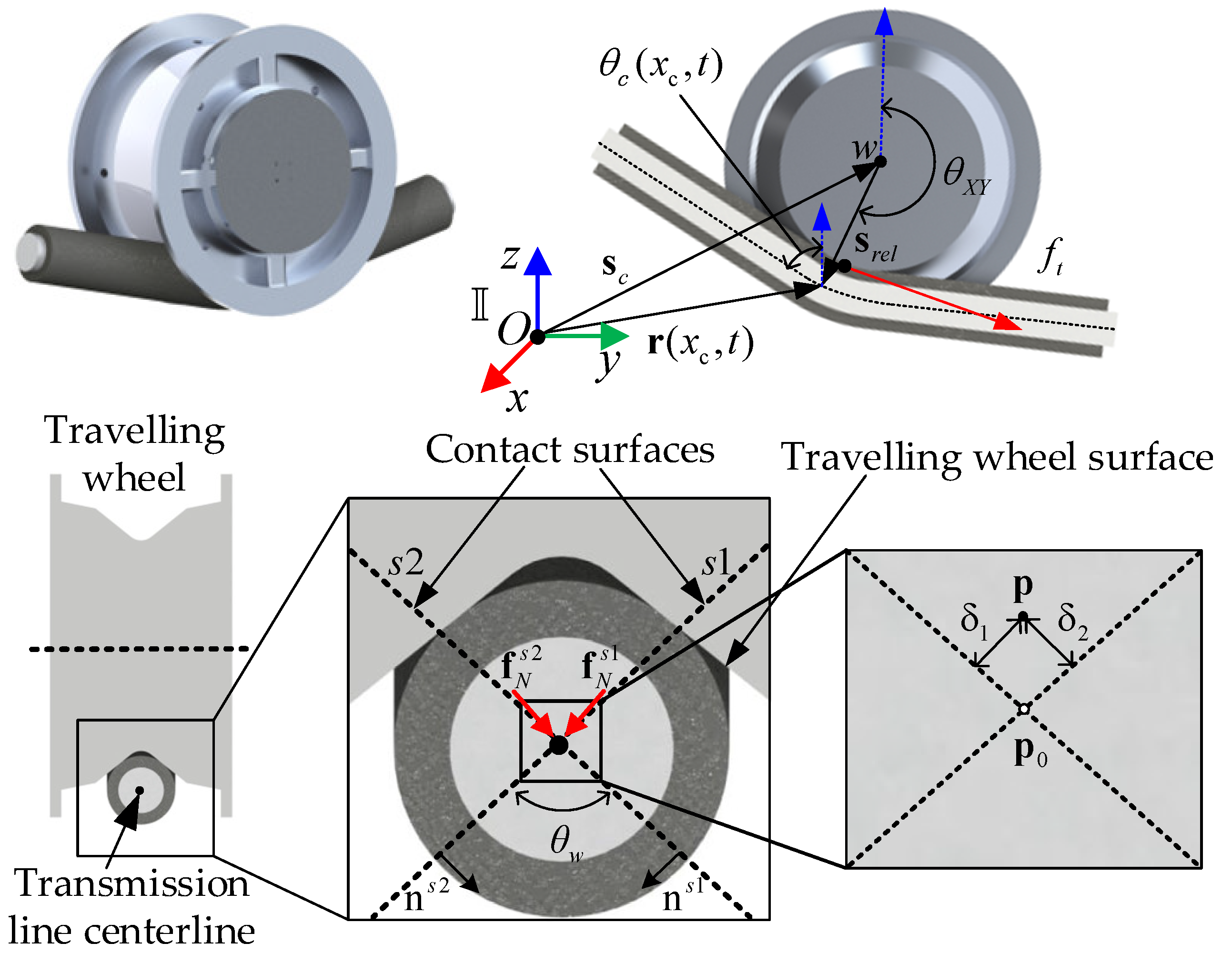
• A coupled FPTLIR/PTL dynamic model was derived to describe the FPTLIR landing process. The PTL was modeled using the ANCF method with a Euler–Bernoulli beam, neglecting shear and torsion to improve computational efficiency. A contact model based on the Hunt–Crossley theory was used to consider the deflection angle of the contact beam element and the traveling wheel groove, to ensure accuracy.
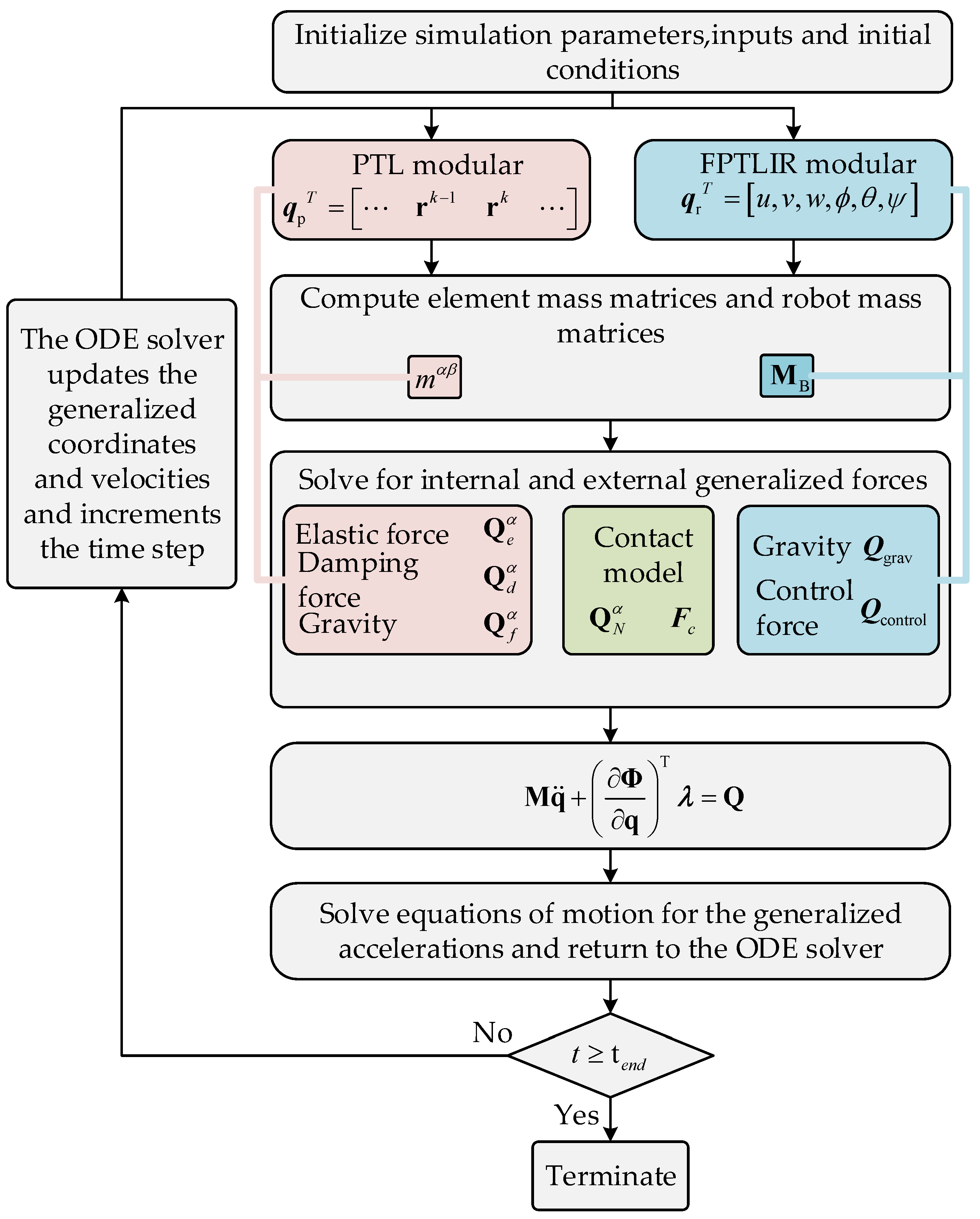
• A modular simulation model was conducted with different landing positions and robot masses to enhance the adaptability and generalization of the model using MATLAB (R2020b) software. The simulation performed parallel updates for the mass matrices of the robot and PTL to improve efficiency, and separated the dynamics calculations of the PTL and the FPTLIR to reduce complexity. The modular design of the simulation enhanced the adaptability to other HIRs.
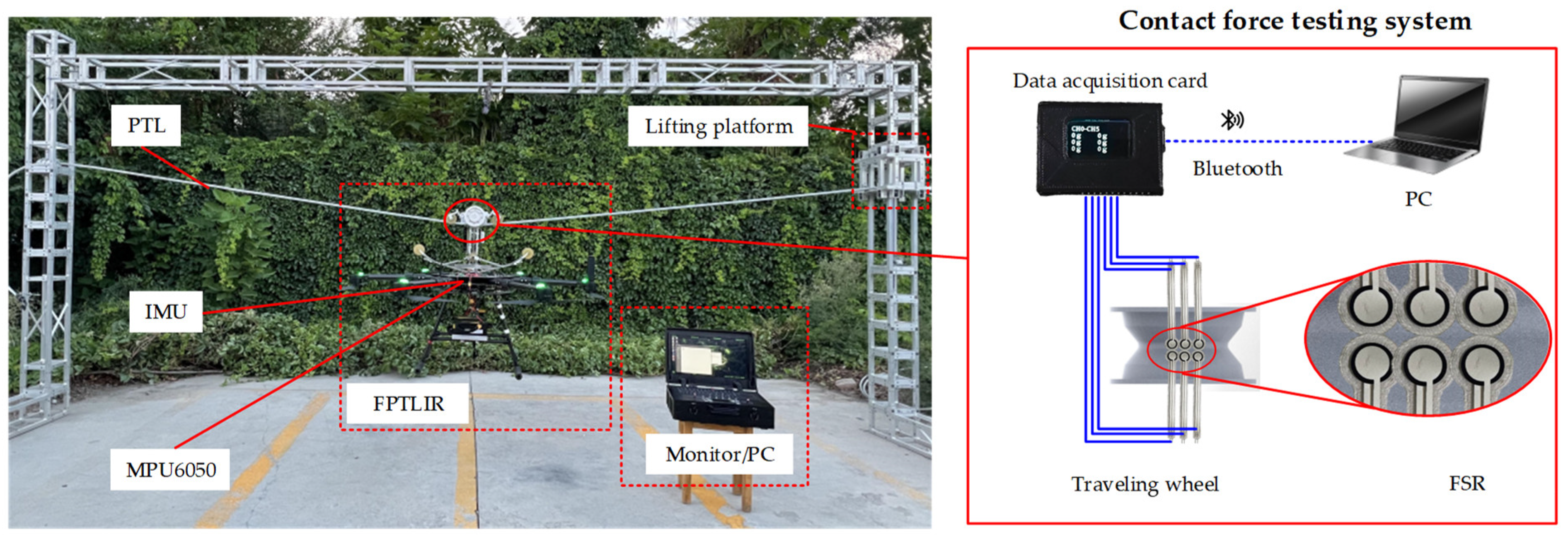
• A comprehensive test platform was established to evaluate the landing performance of the FPTLIR. Six opposing force-sensing resistors (FSRs) were employed on the platform to handle the variability in contact point locations during force measurement. The platform enabled the measurement of attitude, displacements, and contact forces, demonstrating the capability to achieve high measurement accuracy and ensuring reliable evaluation of the proposed method.

The rest of this paper is as follows: Section 2 introduces the operating environment, basic architecture, working principles, and workspace of the FPTLIR. Section 3 explains the constituent elements of the FPTLIR/PTL model. Section 4 presents the results of a simulation and experiment performed on the FPTLIR/PTL system. Section 5 discusses the simulation results in more detail, focusing on the effects of different parameters on the model and the limitations of the current study. The conclusions are summarized in Section 6.

2. Problem Description

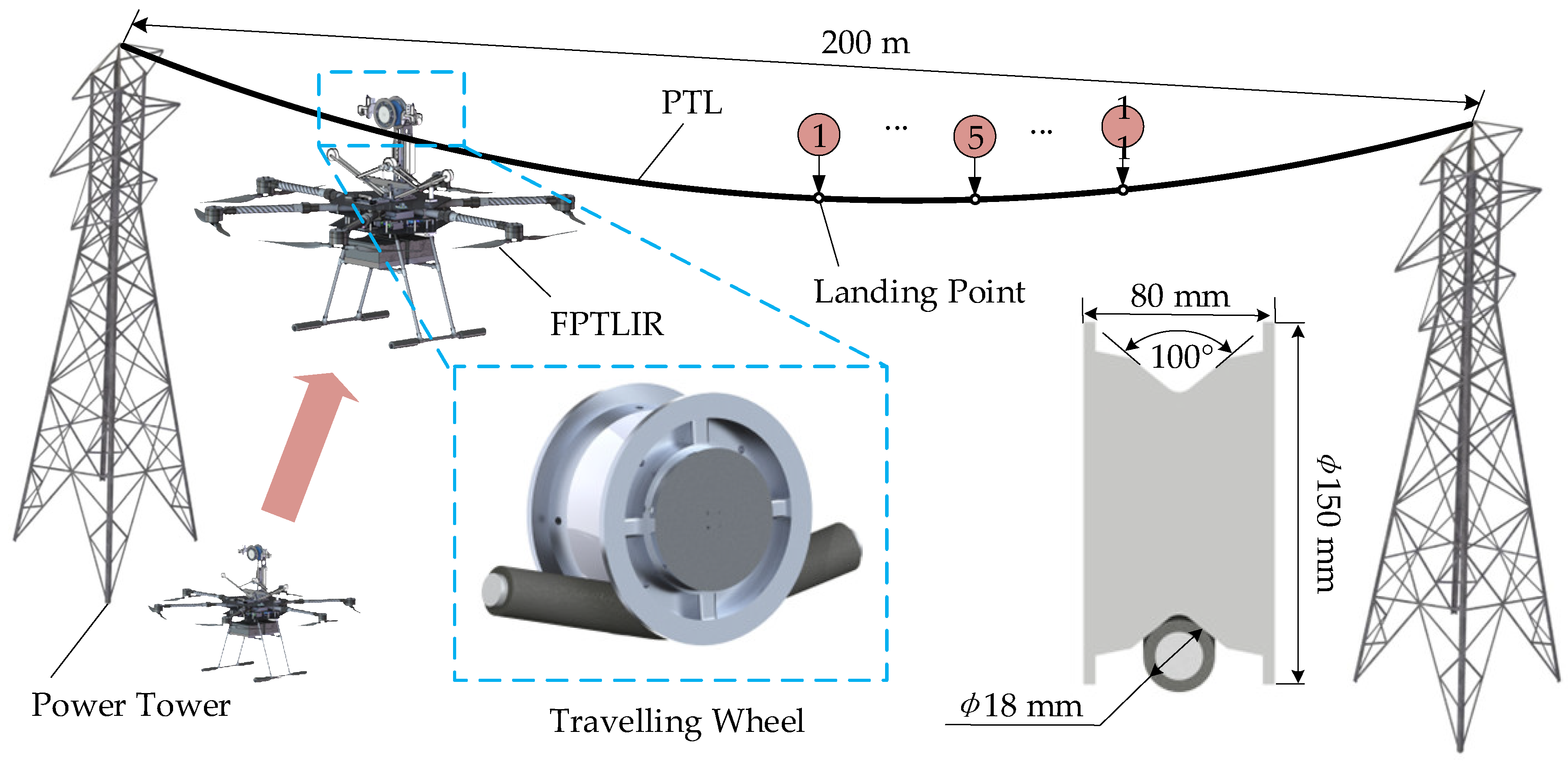
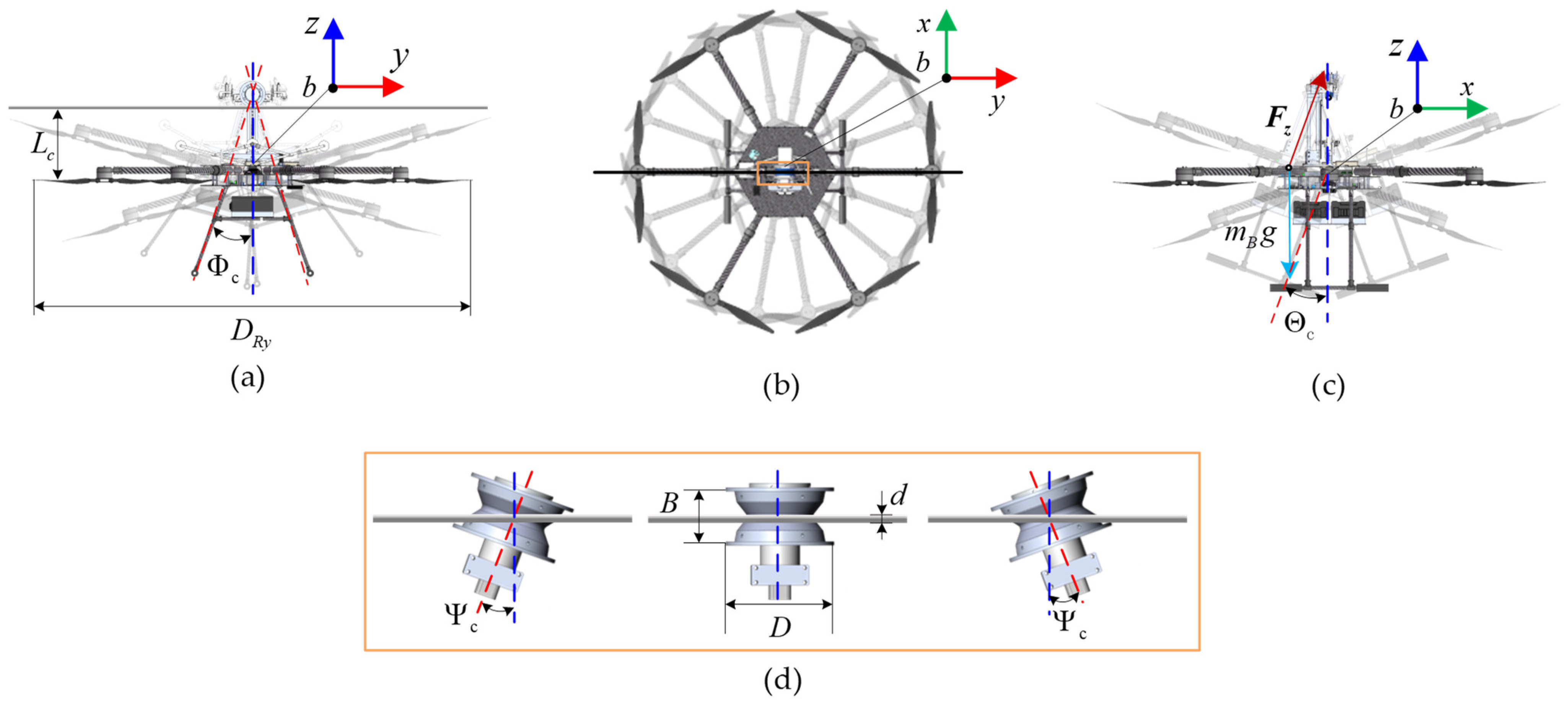
2.1. Description of FPTLIR

HIR mainly consists of a travelling mechanism and a flying mechanism. In some HIRs, the travelling mechanism is placed above the flying mechanism, whereas in others, it is located below it. The travelling mechanism may be either two-wheeled or one-wheeled. This paper focuses on a one-wheeled HIR, specifically the FPTLIR, as the object of study.

The FPTLIR mainly consists of two main components: the flying mechanism and the travelling mechanism, as shown in Figure 1. The flying mechanism is based on a hexacopter drone and includes folding arms, a control chamber, motors, and rotor blades [29]. The travelling mechanism mainly consists of rolling and pressing components. The rolling components include the travelling wheel and auxiliary guide wheels, while the pressing components include the main pressing wheel and auxiliary pressing wheels.

The FPTLIR primarily focuses its inspection along the ground wire, a kind of PTL. The inspection process can be divided into three primary phases: flight landing, walking inspection along the ground wire, and flight detachment. During the flight landing phase, the FPTLIR uses its flying mode to attach itself to the PTL. The robot can choose different points to attach, as shown in Figure 1; the red circle indicates different points, where point 1 is in the middle of the span and point 11 is closer to the power towers. It then switches to the travelling mode to perform the inspection along the PTL. Upon the completion of its multi-span inspection tasks, it returns to flying mode to detach from the PTL and descend to the ground. The groove angle of the travelling wheel is 100°, the width is 80 mm, and the diameter is 150 mm. The diameter of the PTL is 18 mm, and the length is of the span is 200 m. Some key parameters are listed in

Table 1. FPTLIR/PTL system parameters.

Parameter Type	Parameter/Unit	Value
FPTLIR parameters	Mass/kg	38
	Dimension/(mm × mm × mm)	1250 × 1250 × 1200
	Moment of inertia about the x-axis/kg	5.8
	Moment of inertia about the y-axis/kg	5.8
	Moment of inertia about the z-axis/kg	8.5
	Diameter of travelling wheel/mm	150
	Groove angle of travelling wheel/°	100
	Groove width of travelling wheel/mm	80
PTL parameters	PTL length/m	200
	Linear density kg/m	0.91
	Axial stiffness/N/m	8.12 × 107
	Bending stiffness/N·m2	6580
	Diameter/mm	18

.

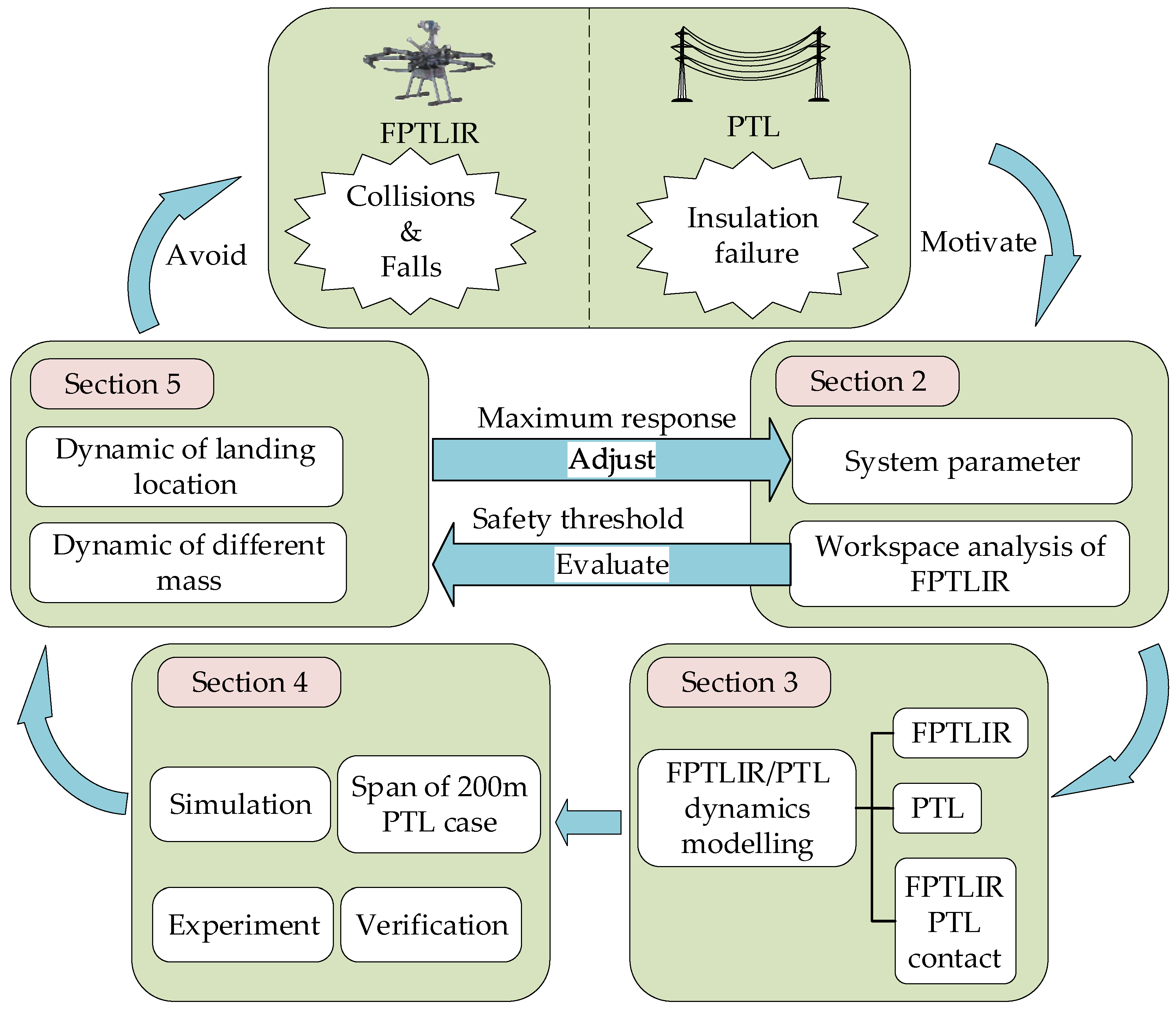
2.2. Overview of the Modeling and Analysis Framework

This framework (Figure 2) starts with failure modes, including robot collisions, falls, and insulation failures. Based on these failure modes, the workspace of the FPTLIR is analyzed by combining the system parameters of the FPTLIR and PTL. These analyses provide a safety threshold to evaluate the dynamic behavior of the FPTLIR. A dynamic model of the interaction between the FPTLIR and PTL is then established. On this basis, simulations and experimental validations are performed to ensure the accuracy and practical feasibility of the model. Finally, the dynamic behavior of the FPTLIR under different landing positions and masses is evaluated, and the maximum response is analyzed to further assess the safety of the FPTLIR during landing. This evaluation provides guidance for adjusting system parameters to prevent failure modes, thereby enhancing overall safety.

2.3. Workspace Analysis of FPTLIR

The workspace analysis of the FPTLIR focuses on evaluating its reachable range and safe zone during the landing process. During the landing process, it is crucial to monitor the robot’s attitude and displacement changes to ensure it does not collide with the PTL, maintains optimal control performance, and avoids compromising the insulation clearance of the PTL. Therefore, quantifying the robot’s workspace provides a foundation for better evaluating its dynamics during and after the landing process, ensuring safe and efficient operation.

Assuming that the local deformation of the PTL is negligible, the analysis of the roll workspace is as follows. When the PTL is horizontal, the roll workspace is as shown in Figure 3a. The width of the robot is $D_{Ry}$, and the distance between the contact point of the lower side of the travelling wheel with the PTL and the rotor plane of the robot is $L_c$. Therefore, when the PTL is horizontal, the safe range of the roll angle is $\left(-{\mathsf{\Phi }}_{\mathrm{c}},{\mathsf{\Phi }}_{\mathrm{c}} \right)$, where ${\mathsf{\Phi }}_{\mathrm{c}}$ is given by:

$${\mathsf{\Phi }}_{\mathrm{c}}=\arctan {\displaystyle \frac{2L_c}{D_{Ry}}}$$

(1)

The robot’s roll workspace varies with the PTL slope. For a 200 m span PTL, its shape and slope distribution are shown in Figure 4a,b The roll workspace at $x$ can be expressed as $\left(-{\mathsf{\Phi }}_{\mathrm{c}}+\alpha (x),{\mathsf{\Phi }}_{\mathrm{c}}+\alpha (x) \right)$, where the PTL shape is fitted by a quadratic function $z=A{x}^2+Bx+C$ and its slope is calculated by $\alpha (x)=\arctan (2Ax+B)$, $\alpha (x)\in (-5.1,5.1)$.

In the yaw motion, the flying mechanism avoids collision with the PTL, but excessive yaw may cause the travelling wheel to detach. With a travelling wheel diameter $D$, inner width $B$, and PTL diameter $d$ (Figure 3d), the safe yaw range $\left(-{\mathsf{\Psi }}_{\mathrm{c}},{\mathsf{\Psi }}_{\mathrm{c}}\right)$ is calculated by:

$$\mathsf{\Psi }c={\tan }^{-1}{\displaystyle \frac{B-d/\cos \mathsf{\Psi }c}{D}}$$

(2)

The formula simplifies to:

$$\mathsf{\Psi }c\approx {\tan }^{-1}{\displaystyle \frac{B-2d}{D}}$$

(3)

For pitch motion, there are no collision constraints as no obstacles exist in this direction. However, excessive pitch can cause significant power loss. Considering the robot’s weight and maximum rotor thrust $F_{z\max }$, the maximum pitch angle is calculated as:

$${\mathsf{\Theta }}_c={\cos }^{-1}{\displaystyle \frac{F_{z\max }}{m_{B}g}}$$

(4)

In power systems, transmission lines consist of phase conductors and ground wires. The robot and PTL1 are safe from flashover when inside the insulation zone (Figure 5). Sufficient spacing between conductors is required to prevent flashover. When the FPTLIR lands on the PTL, its displacement should comply with the following constraints in:

$$Z_c=D_{12}-D_{R\mathrm{z}}-D_E$$

(5)

where $D_{12}$ represents the distance between PTL1 and PTL2, $D_{R\mathrm{z}}$ denotes the geometric height of the FPTLIR, and $D_E$ indicates the safe clearance between PTL1 and PTL2.

By substituting the corresponding values into the derived equations and performing the necessary calculations, the workspace of the FPTLIR is determined. The results, including key parameters and their ranges, are presented in

Table 2. Workspace parameters of the FPTLIR.

Value	Formula	Range
Roll angle	$\left(-{\mathsf{\Phi }}_{\mathrm{c}}+\alpha (x),{\mathsf{\Phi }}_{\mathrm{c}}+\alpha (x) \right)$	$(-19.9,9.1)$$\mathrm{to} (-9.1,19.9)$
Pitch angle	$({\mathsf{\Theta }}_{\mathrm{c}},{\mathsf{\Theta }}_{\mathrm{c}})$	$(-63,63)$
Yaw angle	$\left(-{\mathsf{\Psi }}_{\mathrm{c}},{\mathsf{\Psi }}_{\mathrm{c}}\right)$	$(-16.34,16.34)$
Z-displacement	$\left(0,-Z_c\right)$	$(0,-1.25)$

. This quantified workspace provides a comprehensive understanding of the operational boundaries and serves as a foundation for further analysis of the robot’s dynamics and safety during the landing process.

3. FPTLIR/PTL Dynamics Modelling

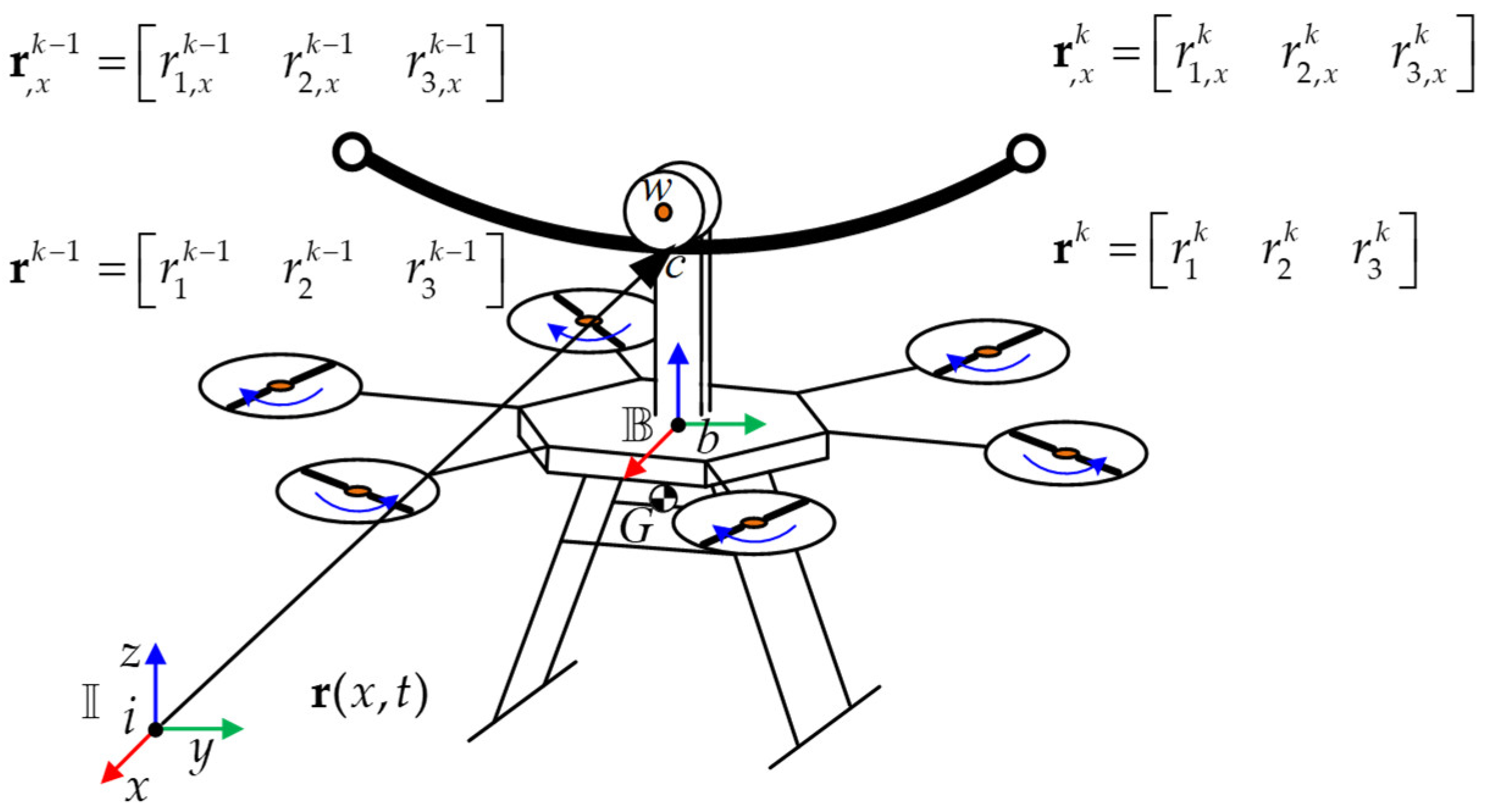
3.1. PTL Modeling

Initially, the PTL is assumed to be unaffected by gravity and concentrated forces. It is typically a multi-layer composite structure. To facilitate calculations, the unstressed PTL is simplified as an Euler–Bernoulli beam with a circular cross-section, neglecting the effects of rotational moments of inertia and shear stress [30]. Given that the initial unstressed total length of the PTL is $L$ and dividing the PTL into $N$ beam units, then the stress-free length of a single element is $l_{\mathrm{e}}=L/N$ and the arc coordinate lengths of the beam node of the unit are $x_j=j{l}_e$ $j=1,2,3,\cdots ,N$ $x_j\in \left[0,L\right]$. Point $b$ is located at the center of the FPTLIR’s rotor plane, which is the origin body reference frame $\mathbb{B}$. The $z$ axes of reference frame $\mathbb{B}$ are orthogonal to the rotor plane. The center of mass of the FPTLIR is indicated by G, and the center of the robot’s travelling wheel is denoted by $w$. The contact point is marked by $c$.

Figure 6 depicts the $k^{th}$ 12-degree element PTL. There are two node coordinates, $r^{k-1}$ and $r^k$, for a $k^{th}$ beam element. The subscript $x$ denotes the first-order derivative with respect to $x$, such as $r_x^k=\partial r^k/\partial x$ and $r_x^{k-1}=\partial r^{j+1}/\partial x$. For subsequent coupling with the FPTLIR, a 6 DOF (degrees of freedom) node is used, where $r_1$, $r_2$, and $r_3$ represent the coordinates of the element node in the X, Y, and Z directions. Within a single element, the global shape function is used to estimate the generalized coordinate vector $r$ at the arc-length coordinate $x$:

$$r(x,t)={\displaystyle \sum _{\alpha =1}^4{s}^{\alpha }}{q}_{\alpha }$$

(6)

where the global shape function is defined as follows, using the Hermite method:

$$s^1=1-3{\xi }^2+2{\xi }^3,s^2=l_{\mathrm{e}}\left(\xi -2{\xi }^2+{\xi }^3\right),s^3=3{\xi }^2-2{\xi }^3,s^4=l_{\mathrm{e}}\left({\xi }^3-{\xi }^2\right)$$

(7)

where $\xi =\left(x-x_{k-1}\right)/l_{\mathrm{e}}$.

The coordinates of a single element can be written as:

$$q_1=r^{k-1}, q_2=r_x^{k-1}, q_3=r^k, q_4=r_x^k$$

(8)

The kinetic energy the $k^{\mathrm{th}}$ element (whose expression is simplified by following Einstein’s summation convention, which eliminates the need for summation symbols) of is formulated as

$$T_k={\displaystyle \frac{1}{2}}{\displaystyle {\int }_{x_{k-1}}^{x_k}{\rho }_A}(x){\dot{r}}^{\mathrm{T}}\dot{r}\mathrm{d}x={\displaystyle \frac{1}{2}}{m}^{\alpha \beta }{\dot{q}}_{\alpha }^{\mathrm{T}}{\dot{q}}_{\beta }$$

(9)

where generalized mass can be computed via:

$$m^{\alpha \beta }={\displaystyle {\int }_{x_{k-1}}^{x_k}{\rho }_A}(x)s^{\alpha }{s}^{\beta }\mathrm{d}x$$

(10)

The linear density, axial stiffness, and bending stiffness of the cable are denoted as: ${\rho }_A$, ${\mathrm{E}}_I$, and $E_{\mathrm{A}}$. The center axis of the element [31], the axial strain of the centroid line, and the material measure of curvature are:

$$\overline{\epsilon }={\displaystyle \frac{1}{2}}\left({\mathbf{r}}_x^{\mathrm{T}}{r}_x-{\overline{r}}_x^T{\overline{r}}_x\right)$$

(11)

$$\mathsf{\kappa }={\displaystyle \frac{‖r_x\times r_{xx}‖}{{‖r_x‖}^2}}$$

(12)

where $\overline{r}$ represents the undeformed vector of the centroid line. When the element is in the initial unstressed configuration, there are $‖{\overline{r}}_x‖=1$. Based on the small deformation assumption, there is $\left|\overline{\epsilon }\right|\ll 1$, $r_x^T{r}_x\approx {\overline{r}}_x^T{\overline{r}}_x$, $\left|\kappa \right|\ll 1$; then, the estimate of curvature at this point is:

$$\kappa \approx ‖r_x\times r_{xx}‖$$

(13)

By transferring Equation (6) to Equations (11) and (13), the axial strain can be expressed as:

$$\overline{\mathsf{\epsilon }}=e^{\alpha \beta }{Q}_{\alpha \beta }$$

(14)

where:

$$Q_{\alpha \beta }={\displaystyle \frac{1}{2}}\left(q_{\alpha }\cdot q_{\beta }-{\overline{q}}_{\alpha }\cdot {\overline{q}}_{\beta }\right)$$

(15)

$$e^{\alpha \beta }=s_x^{\alpha }{s}_x^{\beta }={\displaystyle \frac{s_{\xi }^{\alpha }{s}_{\xi }^{\beta }}{l_{\mathrm{e}}^2}}$$

(16)

The curvature can be approximately expressed by:

$${\kappa }^2\approx {\chi }^{\alpha \beta \mu v}{\tilde{Q}}_{\alpha \beta }{\tilde{Q}}_{\mu v}$$

(17)

where:

$${\chi }^{\alpha \beta \mu \nu }={\displaystyle \frac{1}{l_{\mathrm{e}}^6}}\left[2\left(s_{\xi }^{\alpha }{s}_{\xi }^{\beta }{s}_{\xi \xi }^{\mu }{s}_{\xi \xi }^{\nu }+s_{\xi \xi }^{\alpha }{s}_{\xi \xi }^{\beta }{s}_{\xi }^{\mu }{s}_{\xi }^{\nu }\right)-s_{\xi }^{\alpha }{s}_{\xi \xi }^{\beta }{s}_{\xi }^{\mu }{s}_{\xi \xi }^{\nu }\right.\left.-s_{\xi \xi }^{\alpha }{s}_{\xi }^{\beta }{s}_{\xi }^{\mu }{s}_{\xi \xi }^{\nu }-s_{\xi }^{\alpha }{s}_{\xi \xi }^{\beta }{s}_{\xi \xi }^{\mu }{s}_{\xi }^{\nu }-s_{\xi \xi }^{\alpha }{s}_{\xi }^{\beta }{s}_{\xi \xi }^{\mu }{s}_{\xi }^{\nu }\right]$$

(18)

$${\tilde{Q}}_{\alpha \beta }={\displaystyle \frac{1}{2}}{q}_{\alpha }\cdot q_{\beta }$$

(19)

Based on this, the elastic energy of the $k^{\mathrm{th}}$ element is given as:

$$U_k={\displaystyle \frac{1}{2}}\left(k_{n\epsilon }^{\alpha \beta \mu v}{Q}_{\alpha \beta }{Q}_{\mu v}+k_{n\kappa }^{\alpha \beta \mu v}{\tilde{Q}}_{\alpha \beta }{\tilde{Q}}_{\mu v}\right)$$

(20)

where:

$$k_{n\epsilon }^{\alpha \beta \mu \nu }={\displaystyle {\int }_{x_{k-1}}^{x_k}{E}_A}(x)e^{\alpha \beta }{e}^{\mu \nu }\mathrm{d}x$$

(21)

$$k_{n\kappa }^{\alpha \beta \mu \nu }={\displaystyle {\int }_{x_{k-1}}^{x_k}{E}_I}(x){\chi }^{\alpha \beta \mu v}\mathrm{d}x$$

(22)

The generalized elastic restoring force vector can be computed via:

$$Q_e^{\alpha }=-{\displaystyle \frac{\partial U_k}{\partial q_{\alpha }}}=-\left(k_{n\epsilon }^{\alpha \beta \mu \nu }{Q}_{\mu \nu }+k_{n\kappa }^{\alpha \beta \mu \nu }{\tilde{Q}}_{\mu \nu }\right)q_{\beta }$$

(23)

and furthermore, its Jacobian matrix is formulated as:

$$K_e^{\alpha \beta }=-{\displaystyle \frac{\partial Q_e^{\alpha }}{\partial q_{\beta }}}=\left(k_{n\epsilon }^{\alpha \beta \mu v}{Q}_{\mu \nu }+k_{n\kappa }^{\alpha \beta \mu \nu }{\tilde{Q}}_{\mu \nu }\right)I_3+\left(k_{n\epsilon }^{\alpha \beta \mu \nu }+k_{n\kappa }^{\alpha \beta \mu v}\right)q_{\mu }{q}_v^{\mathrm{T}}$$

(24)

where $I_3$ is a 3 × 3 unit matrix. An internal viscous damping model based on the ANCF method is established for the determination of the energy dissipation of the PTL [22]:

$$Q_d^{\alpha }=-c_d\left(k_{n\epsilon }^{\alpha \beta \mu \nu }{\dot{Q}}_{\mu \nu }+k_{nk}^{\alpha \beta \mu \nu }{\dot{Q}}_{\mu \nu }\right)q_{\beta }$$

(25)

Supposing that a distributed external force, $f(x,t)$, is applied on the $k^{\mathrm{th}}$ element, the generalized external force vector is:

$$Q_f^{\alpha }={\displaystyle {\int }_{x_{k-1}}^{x_k}{s}^{\alpha }}(x)f(x,t)\mathrm{d}x$$

(26)

Self-weight as an external force $f(x,t)={\rho }_{A}g$ (where $g$ is the acceleration of gravity $g=9.8 \mathrm{m}/{\mathrm{s}}^2$), and the gravitational external force vector can be deduced as:

$$Q_f^{\alpha }={\overline{\rho }}_{\mathrm{A}}g{l}_{\mathrm{e}}{\displaystyle {\int }_0^1{s}^{\alpha }}\mathrm{d}\xi$$

(27)

where the mass matrix elements $m^{\alpha \beta }$, $k_{n\epsilon }^{\alpha \beta \mu \nu }$, $k_{n\kappa }^{\alpha \beta \mu \nu }$, and $Q_f^{\alpha }$ are time-independent constants that can be pre-calculated to reduce the amount of computation during simulation.

3.2. FPTLIR/PTL Contact Formulation

The generalized coordinates of the FPTLIR are denoted by ${{\mathit{q}}_r}^T=\left[u,v,w,\varphi ,\theta ,\psi \right]$, and the generalized velocity of the FPTLIR is represented by ${{\dot{\mathit{q}}}_r}^T=\left[\dot{u},\dot{v},\dot{w},\dot{\varphi },\dot{\theta },\dot{\psi }\right]$. The vector from point $b$ to point $i$ is denoted by $u,v,w$. In the inertial coordinate system $\mathbb{I}$, the Euler angles $\varphi ,\theta ,\psi$ represent the rotation of the body coordinate system $\mathbb{B}$ relative to $\mathbb{I}$. In particular, $\psi$ represents the yaw angle, indicating a rotation about the z-axis, $\varphi$ denotes the roll angle, signifying a rotation about the x-axis, and $\theta$ is the pitch angle, denoting a rotation about the y-axis. The rotation matrix from the body coordinate system $\mathbb{B}$ to the inertial coordinate system $\mathbb{I}$ is defined as:

$${\mathit{C}}_{\mathbb{I}}^{\mathbb{B}}=\left[\begin{array}{ccc}c\psi c\theta -s\varphi s\psi s\theta & -c\varphi s\psi & c\psi s\theta +c\theta s\varphi s\psi \\ c\theta s\psi +c\psi s\varphi s\theta & c\varphi c\psi & s\psi s\theta -c\psi c\theta s\varphi \\ -c\varphi s\theta & s\varphi & c\varphi c\theta \end{array}\right]$$

(28)

As the FTPLIR declines, the gap between the travelling wheel and the PTL diminishes until contact is established between the two. During this interaction, the PTL undergoes deformation. The Hunt–Crossley contact model is used to characterize the contact interface as a nonlinear spring-damper system. The contact force per unit length is formulated as:

$${\mathit{f}}_N=k_N{\delta }^n(1+D\dot{\delta })u_N$$

(29)

where $u_N$ is the orthogonal vector perpendicular to the contact surface of the travelling wheel, $k_N$ is the contact stiffness, $\delta$ is the relative penetration depth, $D$ is the contact damping, and $n$ is a positive integer, determined by the local geometric characteristics of the material and the contact surface; it is taken in the current analysis as $n=2.5$ to describe similar constraints [25]. The contact point between the FPTLIR and the PTL is $c$. The arc length coordinate of the corresponding central of the contact point is $x_c$, where $x_k\ge x_c\ge x_{k-1}$. The vector from the center of the travelling wheel $c$ to the contact point on the PTL’s centerline is given by:

$$s_{rel}=r(x_{\mathrm{c}},t)-s_w$$

(30)

where $r(x_{\mathrm{c}},t)$ represents the position of the PTL centerline at the contact point in the inertial coordinate system, and $s_w$ is the position of the travelling wheel center in the inertial coordinate system.

$$s_w=C_{\mathbb{I}}^{\mathbb{B}}\left({\mathit{r}}_{ib}^{\mathbb{B}}+{\mathit{r}}_{bw}^{\mathbb{B}}\right)={\mathit{r}}_{ib}^{\mathbb{I}}+C_{\mathbb{I}}^{\mathbb{B}}{\mathit{r}}_{bw}^{\mathbb{B}}$$

(31)

Then the relative penetration depth is given as:

$$\delta =R+{\displaystyle \frac{d}{2}}-\left|s_{rel}\right|$$

(32)

To accurately describe the contact between the travelling wheel and the PTL, it is necessary to analyze the cross-section at the contact point. The groove surface of the travelling wheel consists of two straight lines. The contact force is applied to the centroid line of the PTL, and the contact area is represented by a dashed line, offset from the actual contact area which is represented by solid lines (Figure 7). The contact planes are denoted by $s1$ and $s2$, intersecting at a point designated as ${\mathbf{p}}_0$. The respective normal vectors of these planes are ${\mathbf{V}}_n^{s1}$ and ${\mathbf{V}}_n^{s2}$.

$${\mathbf{V}}_n^{s1}={\left[0\hspace{0.17em}\hspace{0.17em}\hspace{0.17em}\cos \left({\mathsf{\theta }}_w/2\right)\hspace{0.17em}\hspace{0.17em}\hspace{0.17em}\sin \left({\mathsf{\theta }}_w/2\right)\right]}^T$$

(33)

$${\mathbf{V}}_n^{s2}={\left[0\hspace{0.17em}\hspace{0.17em}\hspace{0.17em}-\cos \left({\mathsf{\theta }}_w/2\right)\hspace{0.17em}\hspace{0.17em}\hspace{0.17em}\sin \left({\mathsf{\theta }}_w/2\right)\right]}^T$$

(34)

The variable ${\mathrm{\theta }}_w$ represents the groove angle of the travelling wheel. The radius of the groove bottom surface of the travelling wheel is smaller than that of the PTL. If the centroid line of the PTL is above one of the dashed lines ($\delta >0$), the normal pressure is proportional to the penetration depth. Conversely, if the centroid line of the PTL is below one of the dashed lines ($\delta <0$), the normal force is zero. Due to the depth limitations of the groove on the travelling wheel, the contact force ceases when the modulus of δ exceeds a certain value. The angle ${\theta }_{XY}$ is defined as the angle between the positive direction of $s_{rel}$ along the z-axis and the yz plane. Since the geometric dimensions of the beam element are much larger than those of the travelling wheel, the influence of the FPTLIR’s contact process on the tilt angle of the beam element can be considered to be negligible. Consequently, ${\theta }_{XY}$ can be approximated as follows:

$${\theta }_{XY}={\displaystyle \frac{3}{2}}\pi -\theta \left(x_c,t\right)$$

(35)

Here, $\theta \left(x_c,t\right)$ is the angle of the contact beam element in yz plane relative to the positive direction of the z-axis, which can be written as:

$$\theta \left(x_c,t\right)=\arccos \left({\displaystyle \frac{\frac{\partial r_2}{\partial x}}{\sqrt{{\left(\frac{\partial r_2}{\partial x}\right)}^2+{\left(\frac{\partial r_3}{\partial x}\right)}^2}}}\right)$$

(36)

The normal vector of the contact plane in the inertial frame can be expressed by:

$$u_N=C_{\mathbb{I}}^{\mathbb{B}}{R}_y{\left({\theta }_{YZ}\right)}^{-1}\mathbf{V}$$

(37)

where:

$$R_y\left({\theta }_{YZ}\right)=\left[\begin{array}{ccc}\cos {\theta }_{YZ}& 0& \sin {\theta }_{YZ}\\ 0& 1& 0\\ -\sin {\theta }_{YZ}& 0& \cos {\theta }_{YZ}\end{array}\right]$$

(38)

In the absence of external forces, the initial configuration of the PTL is determined by gravity alone, resulting in a catenary shape. As the FPTLIR descends, it forms an angle with the PTL. If this angle exceeds a critical threshold, the FPTLIR may slide downward along the PTL. Considering only the tangential $t$ interaction force between the FPTLIR and the PTL within the yz plane, the unit tangential vector at the contact point is ${\mathit{V}}_t$, which is perpendicular to the vector $s_{rel}$. The generalized contact force can be calculated as:

$$Q_N^{\alpha }=s^{\alpha }(\eta ){\mathit{F}}_c$$

(39)

Given that the minimum bending radius of the PTL is considerably larger than that of the travelling wheel, it is reasonable to assume that the contact length, represented by the variable $l_0$, remains constant over time. The contact force in the inertial coordinate system $\mathbb{I}$ is expressed as:

$${\mathit{F}}_c={\displaystyle {\mathbf{\int }}_0^{l_0}\left({\mathit{f}}_N^{s1}+{\mathit{f}}_N^{s2}+{\mathit{f}}_t\right)dx}$$

(40)

The tangential friction force is formulated as:

$${\mathit{f}}_t={\mathit{V}}_t\mu \left(\left|{\mathit{f}}_N^{s1}\right|+\left|{\mathit{f}}_N^{s2}\right|\right)$$

(41)

where:

$$\eta ={\displaystyle \frac{x_c-x_{k-1}}{l_{\mathrm{e}}}}$$

(42)

During the attachment phase of the FPTLIR’s flight, the travelling wheels are in a braking state, preventing any relative rotation between the wheels and the FPTLIR. Consequently, in the absence of relative sliding between the travelling wheels and the PTL, the arc length coordinate $x_c$ remains constant over time. Within the global coordinate system, as the FPTLIR stabilizes during its descent, the contact points remain aligned on the contact plane, ensuring no penetration or separation between the FPTLIR and the PTL. The kinematic constraints imposed by the contact can be written as:

$${{\mathit{V}}_t}^{\mathrm{T}}(r^w-r^r)=0$$

(43)

The global position vectors of the contact point on the PTL and the travelling wheel are respectively denoted by $r^w$. It is assumed that the coordinates of the contact point on the PTL and the travelling wheel are known. In this case, the kinematic constraint equation can be derived from the PTL equation, which defines the tangential and normal vectors as functions of the PTL. This is shown in Equation (38).

3.3. FPTLIR Subsystem Dynamics

The moment of inertia of the FPTLIR in the body coordinate system is calculated using the parallel axis theorem as follows:

$${\mathit{I}}_{GB}^{\mathbb{B}}={\mathit{I}}_{bB}^{\mathbb{B}}+m_{\mathrm{B}}\left[({\mathit{r}}_{bG}^{\mathbb{B}}\times {\mathit{r}}_{bG}^{\mathbb{B}}){\mathit{I}}_3-{\mathit{r}}_{bG}^{\mathbb{B}}\otimes {\mathit{r}}_{bG}^{\mathbb{B}}\right]$$

(44)

In this context, ${\mathit{r}}_{bG}^{\mathbb{B}}$ represents the displacement vector from the FPTLIR’s center of mass to its center of gravity. The symbol $\otimes$ denotes the cross product, and $I_{bB}^{\mathbb{B}}$ is a diagonal matrix containing the principal moments of inertia $I_x$, $I_{\mathrm{y}}$, and $I_{\mathrm{z}}$:

$${\mathit{I}}_{bB}^{\mathbb{B}}=\left[\begin{array}{ccc}{I}_x& 0& 0\\ 0& I_y& 0\\ 0& 0& I_z\end{array}\right]$$

(45)

The angular velocity and linear velocity in Equation (44) can be expressed in terms of the FPTLIR’s generalized velocity, as outlined in reference [32]:

$${\displaystyle \frac{d}{dt}}{\left({\mathit{r}}_{ib}^{\mathbb{B}}\right)}_{\mathbb{I}}={\mathit{J}}_{ib,D}^{\mathbb{B}}{\dot{\mathit{q}}}_r$$

(46)

$${\mathit{\omega }}_{\mathbb{I}\mathbb{B}}^{\mathbb{B}}={\mathit{J}}_{\mathbb{I}\mathbb{B},R}^{\mathbb{B}}{\dot{\mathit{q}}}_r$$

(47)

where:

$$J_{ib,D}^{\mathbb{B}}=\left[\begin{array}{cc}{C}_{\mathbb{I}}^{\mathbb{B}}& 0_{3\times 3}\end{array}\right]$$

(48)

$${\mathit{\omega }}_{\mathbb{I}\mathbb{B}}^{\mathbb{B}}=\left[\begin{array}{ccc}1& 0& -\mathrm{s}(\theta )\\ 0& \mathrm{c}(\varphi )& \mathrm{s}(\varphi )\mathrm{c}(\theta )\\ 0& -\mathrm{s}(\varphi )& \mathrm{c}(\theta )\mathrm{c}(\varphi )\end{array}\right]\left[\begin{array}{c}\dot{\varphi }\\ \dot{\theta }\\ \dot{\psi }\end{array}\right]={\mathit{C}}_{\varphi \theta }^{{\overrightarrow{\omega }}_{\mathbb{I}\mathbb{B}}^{\mathbb{B}}}\left[\begin{array}{c}\dot{\varphi }\\ \dot{\theta }\\ \dot{\psi }\end{array}\right]$$

(49)

$${\mathit{J}}_{\mathbb{I}\mathbb{B},\mathit{R}}^{\mathbb{B}}=\left[\begin{array}{cc}{0}_{3\times 3}& C_{\varphi \theta }^{{\mathit{\omega }}_{\mathbb{I}\mathbb{B}}^{\mathbb{B}}}\end{array}\right]$$

(50)

$${\displaystyle \frac{d}{dt}}{\left({\mathit{r}}_{iG}^{\mathbb{B}}\right)}_{\mathbb{I}}=\left({\mathit{J}}_{ib,D}^{\mathbb{B}}-\left[{\mathit{r}}_{bG}^{\mathbb{B}}\right]\times {\mathit{J}}_{\mathbb{I}\mathbb{B},R}^{\mathbb{B}}\right){\dot{\mathit{q}}}_r=J_{iG,D}^{\mathbb{B}}{\dot{\mathit{q}}}_r$$

(51)

$$T_B={\displaystyle \frac{1}{2}}{{\dot{\mathit{q}}}_r}^T{M}_B{\dot{\mathit{q}}}_r$$

(52)

where $M_B$ can be defined as:

$$M_B=m_B{\mathit{J}}_{iG,D}^{\mathbb{B}}{}^T\mathit{J}_{iG,D}^{\mathbb{B}}+{{\mathit{J}}_{\mathbb{B},R}^{\mathbb{B}}}^T\left({\mathit{I}}_{bB}^{\mathbb{B}}+m_B{\left[{\mathit{r}}_{bG}^{\mathbb{B}}\right]}_{\mathrm{x}}^2\right){\mathit{J}}_{\mathbb{I}\mathbb{B},R}^{\mathbb{B}}$$

(53)

The control vector of the FPTLIR is written as:

$${\mathit{F}}_{\mathbb{B}}={\left[\begin{array}{llllll}0\hfill & 0\hfill & F_z^{\mathbb{B}}\hfill & M_x^{\mathbb{B}}\hfill & M_y^{\mathbb{B}}\hfill & M_z^{\mathbb{B}}\hfill \end{array}\right]}^T$$

(54)

Therefore, the kinetic energy of the FPTLIR can be derived as:

$$T_B={\displaystyle \frac{1}{2}}\left(m_B{\displaystyle \frac{d}{dt}}{\left({\mathit{r}}_{iG}^{\mathbb{B}}\right)}_{\mathbb{I}}^T{\displaystyle \frac{d}{dt}}{\left({\mathit{r}}_{iG}^{\mathbb{B}}\right)}_{\mathbb{I}}+{\left({\mathit{\omega }}_{\mathbb{I}\mathbb{B}}^{\mathbb{B}}\right)}^T{I}_{GB}^{\mathbb{B}}{\mathit{\omega }}_{\mathbb{I}\mathbb{B}}^{\mathbb{B}}\right)$$

(55)

where velocity of the FPTLIR’s center of mass is:

$${\displaystyle \frac{d}{dt}}{\left({\mathit{r}}_{iG}^{\mathbb{B}}\right)}_{\mathbb{I}}={\displaystyle \frac{d}{dt}}{\left({\mathit{r}}_{ib}^{\mathbb{B}}\right)}_{\mathbb{I}}+{\displaystyle \frac{d}{dt}}{\left({\mathit{r}}_{bG}^{\mathbb{B}}\right)}_{\mathbb{I}}={\displaystyle \frac{d}{dt}}{\left({\mathit{r}}_{ib}^{\mathbb{B}}\right)}_{\mathbb{I}}+{\mathit{\omega }}_{\mathbb{I}\mathbb{B}}^{\mathbb{B}}\times {\mathit{r}}_{bG}^{\mathbb{B}}$$

(56)

3.4. Calculation of the Motion Equations of the System

The equations of motion for the FPTLIR can be obtained using the Lagrange equation as follows:

$${\displaystyle \frac{\mathrm{d}}{\mathrm{d}t}}\left({\displaystyle \frac{\partial T_B}{\partial {\dot{\mathit{q}}}_r}}\right)-{\displaystyle \frac{\partial T_B}{\partial {\mathit{q}}_r}}={\mathit{Q}}_{grav}+{\mathit{Q}}_{\mathrm{con} }+{\mathit{F}}_c$$

(57)

Substituting Equation (52) into Equation (57) yields:

$$M_{\mathrm{B}}{\ddot{q}}_{\mathrm{r}}={\mathit{Q}}_{\mathrm{grav}}+{\mathit{Q}}_{\mathrm{con} }+{\mathit{F}}_c$$

(58)

The gravitational force acting on the FPTLIR in the inertial coordinate system is given by ${\mathit{Q}}_{\mathrm{grav}}=m_B{\mathit{g}}^{\mathbb{I}}$, and the control force in the inertial coordinate system is:

$${\mathit{Q}}_{\mathrm{con} }={\left[\begin{array}{l}{\mathit{J}}_{ib,D}^{\mathbb{B}}\hfill \\ {\mathit{J}}_{\mathbb{I}\mathbb{B},R}^{\mathbb{B}}\hfill \end{array}\right]}^T{\left[\begin{array}{llllll}0\hfill & 0\hfill & {\mathit{F}}_{\mathrm{z}}^{\mathbb{B}}\hfill & {\mathit{M}}_x^{\mathbb{B}}\hfill & {\mathit{M}}_y^{\mathbb{B}}\hfill & {\mathit{M}}_z^{\mathbb{B}}\hfill \end{array}\right]}^T$$

(59)

This study investigates the system’s performance under the condition of no external intervention, where the control force is set to zero. The PTL is suspended at both ends by rigid insulators attached to power towers, which impose fixed constraints on the system at both ends. The generalized coordinates of the FPTLIR are constrained by the contact point with the PTL. Since the relative deformation of the insulators is negligible, it is not considered in this analysis. The kinematic constraints are incorporated into the constraint equations pertaining to the generalized coordinates of $q$. The matrix $q$ comprises the complete set of elements, $q_{\alpha }$. Therefore, the govern equations for the entire system are formulated using the Lagrange equation and a set of constraint equations, as follows:

$$M\ddot{q}+{\left({\displaystyle \frac{\partial \mathbf{\Phi }}{\partial q}}\right)}^{\mathrm{T}}\mathit{\lambda }=Q$$

(60)

$$\mathbf{\Phi }(q)=0$$

(61)

In the above equation, the matrix $M$ is constituted by the mass matrix of the PTL $m^{\alpha \beta }$ and the mass matrix of the FPTLIR $M_{\mathrm{B}}$. The coefficient matrix of the constraint equation is represented by $\mathbf{\Phi }$, while the vector of Lagrange multipliers is represented by $\mathit{\lambda }$. The generalized force, denoted by $Q$, is a function of the previously calculated forces $Q_e^{\alpha }$, $Q_f^{\alpha }$, $Q_N^{\alpha }$, ${\mathit{Q}}_{grav}$, ${\mathit{Q}}_{\mathrm{con} }$, and ${\mathit{F}}_c$.

4. Simulation and Experiment

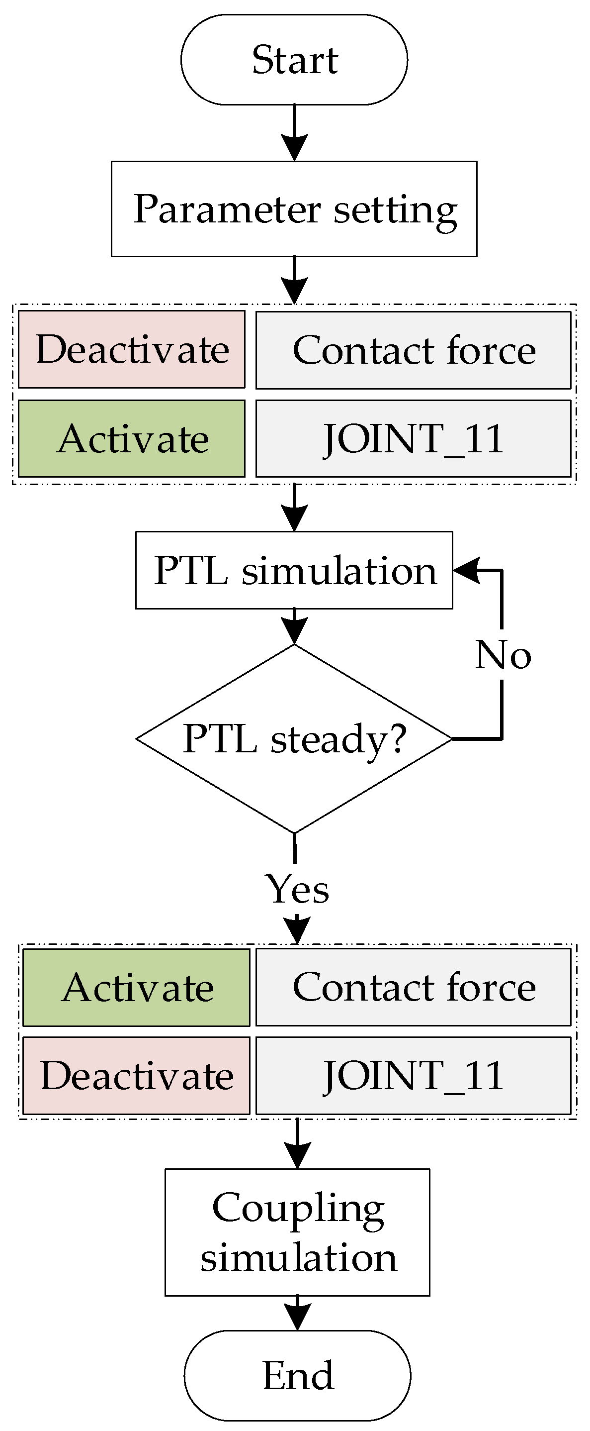
4.1. Dynamic Simulation Workflow

To achieve precise simulation of the dynamic behavior of the PTL and FPTLIR, a modular simulation was employed, dividing the simulation process into two main modules, where the red represented the PTL module, and the blue represented the FPTLIR module (Figure 8). First, during the initialization phase, global simulation parameters (e.g., total simulation time and time step size) were defined, the generalized coordinates and initial conditions for both the PTL and FPTLIR systems were set, and geometric and physical models that met actual operational requirements were constructed. Next, the mass matrices of the PTL and FPTLIR were computed in parallel. The mass matrix of the PTL remained constant, while that of the FPTLIR dynamically updated according to its varying attitudes. Following this, the internal and external generalized forces of the PTL and FPTLIR systems were computed in parallel. The internal forces of the PTL included elastic and damping forces, while the external forces consisted of gravity and contact forces. The external forces acting on the FPTLIR included contact forces and control forces, which were updated at each iterative step. The green-colored contact model dynamically updated contact forces in real time based on the arc coordinates of the PTL’s contact points and the generalized coordinates of the FPTLIR. These forces were computed in independent modules and integrated into the system’s equations of motion. Subsequently, the equations of motion module combined the mass matrix and generalized forces to form the system’s dynamic equations (Equations (60) and (61)), which were solved separately using the generalized-α method. This method optimized energy dissipation characteristics by adjusting parameters, ensuring high accuracy and numerical stability during temporal integration. Based on the generalized-α method, the generalized velocity and displacement at the current time step were calculated, the system state was updated, and the simulation time step was dynamically adjusted during periods of rapid change to enhance efficiency and accuracy. Throughout the simulation process, system response indicators (e.g., displacement and force) were continuously evaluated, and the simulation was terminated based on predefined conditions. The results were then output for further analysis.

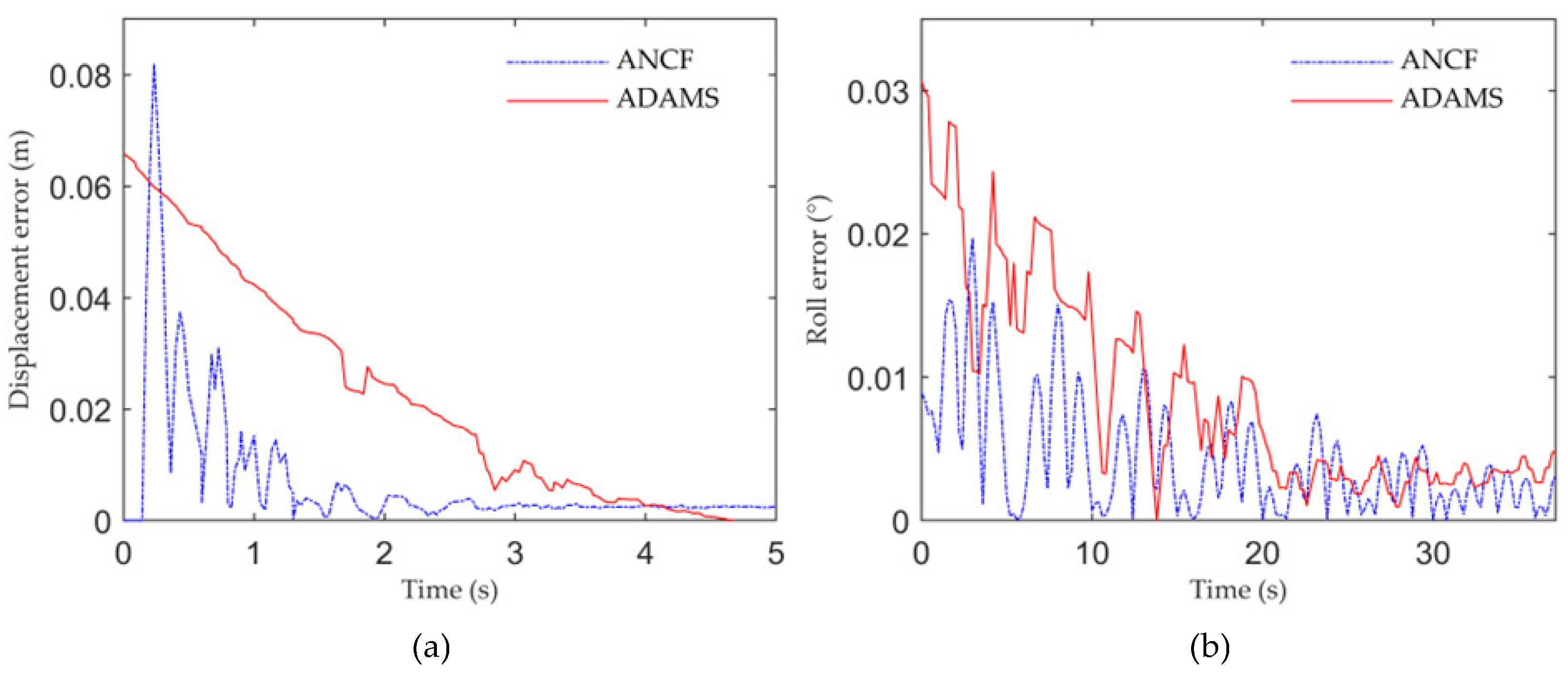
4.2. Comparison of Different Methods

The dynamic system was also modeled using the ADAMS 2020 software (Figure 9) and the results of the numerical simulation were compared. A simplified FPTLIR model was constructed within the software with two parts. The 10 m PTL was modeled using the finite element (FE) model with 20 nodes, a damping ratio of stiffness set to 0.03, mass set to 1.0, material density set to 3595 kg/m³, elastic modulus set to 79.8 GPa, and Poisson’s ratio set to 0.4. The main contact parameters were configured as follows: force exponent set to 2.5, contact damping set to $1\times {10}^4$, penetration depth set to 0.01 m, and static friction coefficient set to 0.7. JOINT_8 and JOINT_9 were fixed constraints applied to both ends of the PTL, while JOINT_10 represented the fixed constraint between the travelling wheel and the FPTLIR, ensuring that the travelling wheel remained locked during landing to prevent slippage. The contact force represented the interaction between the travelling wheel and the PTL.

The simulation workflow is shown in the Figure 10. The PTL was initially configured as a straight line without external forces. After stabilization under gravitational forces, the sag of the PTL at the specified landing point was obtained, and the FPTLIR was positioned accordingly. The simulation then proceeded as follows: first, the contact force was deactivated, and JOINT_11 was activated; after the PTL reached a steady state and was positioned below the travelling wheel, the contact force was activated, and JOINT_11 was deactivated, completing the coupled simulation.

A comparison of results between the ANCF method and FEM method in ADAMS is shown in Figure 11. In the case study, the PTL length was set to 10 m, with the robot descending from the midpoint. The simulation parameters were consistent with the experimental setup, and the errors between the simulation results of the two methods and the experimental values were analyzed. Since the baseline values of the pitch and yaw angles were relatively small, our comparison focuses on the more dynamic roll angle and the displacement in the Z direction.

As shown in Figure 11a, the Z-displacement error of the ANCF method stabilized quickly and remained below 0.02 m after 1 s, while the FEM exhibited larger fluctuations and remained below 0.02 m after 2 s. Similarly, Figure 11b indicated that the roll error of the ANCF method consistently stayed below 0.01° after 10 s, while the FEM demonstrated greater oscillations throughout the simulation. In terms of average errors, the Z-displacement average error of ANCF method was 0.005 m, compared to 0.014 m for FEM, representing a 64% error reduction. The average roll error of ANCF method was measured at 0.004°, whereas FEM exhibited 0.008°, indicating a 50% reduction in average error.

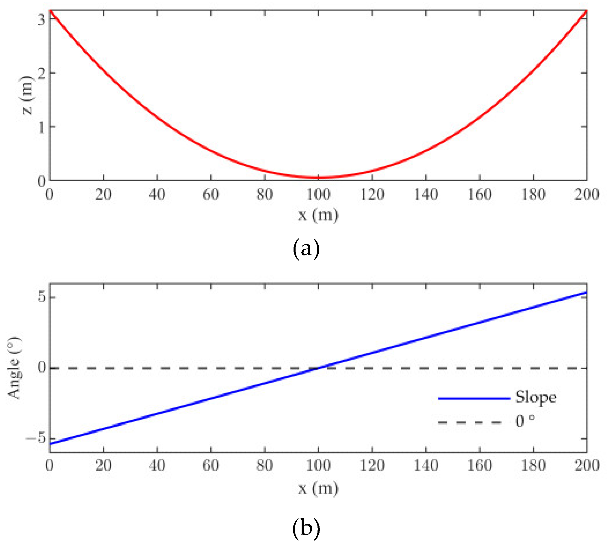
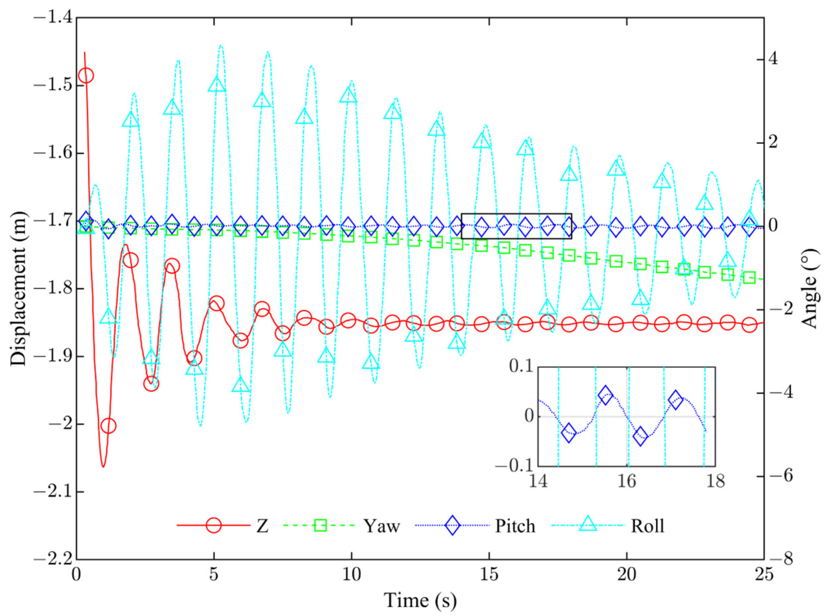
4.3. Span of 200 m PTL Case

The span of PTLs typically ranges from 100 to 200 m. To further investigate the dynamic performance of the robot on long-span PTLs, a PTL with a span of 200 m was specified. The elastic modulus was set to 79.8 GPa, the diameter to 18 mm, and the linear density to 0.91 kg/m. The bending stiffness and axial stiffness could be derived from these parameters. The initial configuration of the PTL was set without any stretching, maintaining its original length. The simulation was run for 2 s with a convergence criterion of $1\times {10}^{-3}$. A total of 20 nodes were set up for the simulation. The initial condition for the FPTLIR’s descent was set by establishing the steady state of the PTL. The FPTLIR was designed to descend from point 9 of the PTL, with the centerline of the FPTLIR’s travelling wheels aligned with the centerline of the PTL in the yz plane.

To analyze the dynamic behaviors of the system, Figure 12 shows the Z-displacement of the FPTLIR and the variations in attitude angles (yaw, pitch and roll) during and after the descent. As the displacements in the X and Y directions during the descent were negligible, they were not included in the data collection.

During the initial phase, the Z-displacement stabilized at −1.45 m, indicating the steady-state condition where the PTL was only affected by gravity, with no interaction between the FPTLIR and the PTL. Then, within the time frame of 0–0.9 s, the FPTLIR rapidly descended to reach a peak value of −3.3 m due to gravitational forces. Thereafter, the Z-displacement oscillated around −2.0 m. Following 9.8 s, upon the interaction between the PTL and the FPTLIR beginning, the Z-displacement finally stabilized at −1.8 m.

The attitude angles exhibited varying amplitudes and oscillation frequencies. The roll angle started at 0°, increased with amplified oscillations to a peak at 4.47 s, and transitioned to periodic fluctuations as the Z-displacement stabilized. This behavior can be attributed to the transformation of the system into a universal pendulum model after stabilization of the Z-displacement. Similarly, single-arm robotic structures also show an initial surge in roll angles at the start of the walking phase, followed by damped oscillations [33].

The yaw angle gradually rose from 0°, reaching −1.2° at 25 s. This change occurred slowly and without oscillation, showcasing the robust coupling between the yaw angle and the PTL. The PTL’s integration into the FPTLIR’s wheels ensured steady changes over time. The pitch angle exhibited oscillations between −0.1° and 0.1°, with minimal amplitude variations.

These differences in amplitude levels arose from varying constraints and the FPTLIR’s principal moments of inertia. The principal moment of inertia in the Z direction was the largest for the robot, and the constraints were also the strongest, resulting in minimal yaw angle fluctuations. In the X and Y directions, the moments of inertia were identical. During zero-velocity landing, the robot was mainly affected by gravity, resulting in no excitation in the Y direction. Consequently, compared to roll, the pitch fluctuation was much smaller, although its fluctuation frequency was similar to that of roll.

The roll angle initially stabilized during oscillations, with the oscillation period gradually increasing. Once stabilization occurred, variations in the FPTLIR’s attitude angles had a negligible impact on the Z-displacement.

The FPTLIR’s descent at a point 9 demonstrates the relationship between the Z-displacement, pitch angle, yaw angle, and roll angle as they change over time during the descent. Nevertheless, it should be noted that in some cases, descending at that point may not be a necessary action for the FPTLIR when operating on the PTL. Instead, the FPTLIR may descend at other points along the PTL. It was therefore essential to carry out a detailed study and comparison of the dynamic characteristics of the FPTLIR’s descent at different points along the PTL during the inspection process.

To facilitate a comparative analysis of the dynamic behavior of the system as the FPTLIR descended at different points, several descent points were established to evaluate the dynamic performance of the system. As the PTL was positioned horizontally at a constant height and its sides were symmetrical, only the descent behavior at different points along one side of the PTL was examined. In a 200-metre long PTL, simulation experiments were carried out by placing a descent point at 10-metre intervals along one side over a length of 100 m.

To enable a comparative analysis of the FPTLIR’s Z-displacement at different landing sites, the relative change in displacement was calculated by subtracting the pre-landing steady-state displacement from the post-landing dynamic displacement. Figure 13a shows that the Z-displacement of the FPTLIR reached a peak value at each landing point, followed by oscillatory behavior. As the landing point approached the tower, the peak displacement and the time to reach stability decreases. This phenomenon is due to the increased tension in the PTL as the landing point approaches the tower, which reduced the deformation caused by external disturbances and accelerated the stabilization process.

When the FPTLIR landed at different points, the variation patterns of each attitude angle remained unchanged compared to those at point 9. To clearly see the attitude change of different points, the initial 20 s of data are shown in Figure 13b–d. The frequency of the pitch angles remained relatively constant across the different contact locations and its value fluctuated within the range of −0.04° to 0.06° across the different contact points. The pitch angle had the highest frequency, followed by the roll angle. The roll angle decreased over time and increased as the FPTLIR approached the tower.

To clarify the factors contributing to the variations in the FPTLIR’s Z-displacement and attitude angles at different landing points, the landing point was set at the midpoint. The horizontal stress variations of the PTL at different points along the line were then recorded, as shown in Figure 14.

The minimum stress was located in the central region of the PTL, while the maximum stress can be observed near the tower within the static condition at time 0 s. The stress distribution generally showed a progressive escalation from the center towards the tower. The static analysis shows a rapid increase in stress from point 0 to point 3, followed by a more gradual increase, culminating in a pronounced escalation after point 10. As seen in the dynamic results, the stress at point 0 first increased to a peak, then underwent fluctuations before reaching stability at 7.1 s. At the same time, as the landing site approached the tower, the stress magnitude increased, the fluctuation amplitude decreased and the attainment of stability was accelerated. After the FPTLIR’s landing stabilization, the total stress across the PTL increased to an elevated state.

To investigate the dynamic behavior of the FPTLIR during descent over different masses, the study considered FPTLIRs ranging from 15 kg to 100 kg, as referred to in [11,34]. The mass of the FPTLIR was systematically varied from 10 kg to 100 kg, specifically set at 10 kg, 55 kg, and 100 kg for different simulation experiments. The FPTLIRs were consistently programmed to land at point 9. This analysis compared the dynamic performance of FPTLIRs with different masses during their descent. It was hypothesized that variations in mass would be due to changes in FPTLIR density, and consequently have a linear effect on the rotational dynamics of the FPTLIR.

The simulation results in Figure 15 indicate the different dynamic responses of FPTLIRs under varying conditions of mass (10 kg, 55 kg, and 100 kg). The Z-displacement variation with different FPTLIR masses is shown in Figure 15a. Specifically, a 10 kg FPTLIR had a maximum Z-displacement of −0.56 m, while an FPTLIR of 55 kg mass and a 100 kg mass had displacements of −0.87 m and −1.15 m, respectively. It is evident that heavier FPTLIRs required more time to reach a stable state. It can be observed that an increase in mass had a proportional impact on the PTL, resulting in a corresponding increase in Z-displacement. Figure 15b–d illustrate that the amplitude of post-landing attitude oscillations increased with the mass of the FPTLIR. Specifically, raising the mass from 10 kg to 100 kg led to a significant rise in the roll angle from −1.0° to −7.84°, and the yaw angle from −0.09° to −0.65°, while the pitch angle remained unaffected by the mass, consistently oscillating between −0.05° and 0.05°. The motion patterns of each angular parameter remained unchanged with varying mass; pitch exhibited oscillation, roll showed oscillatory decay, and yaw gradually increased. However, the amplitude uniformly increased as mass grew, attributed to the larger moments of inertia, which amplified the oscillation magnitude.

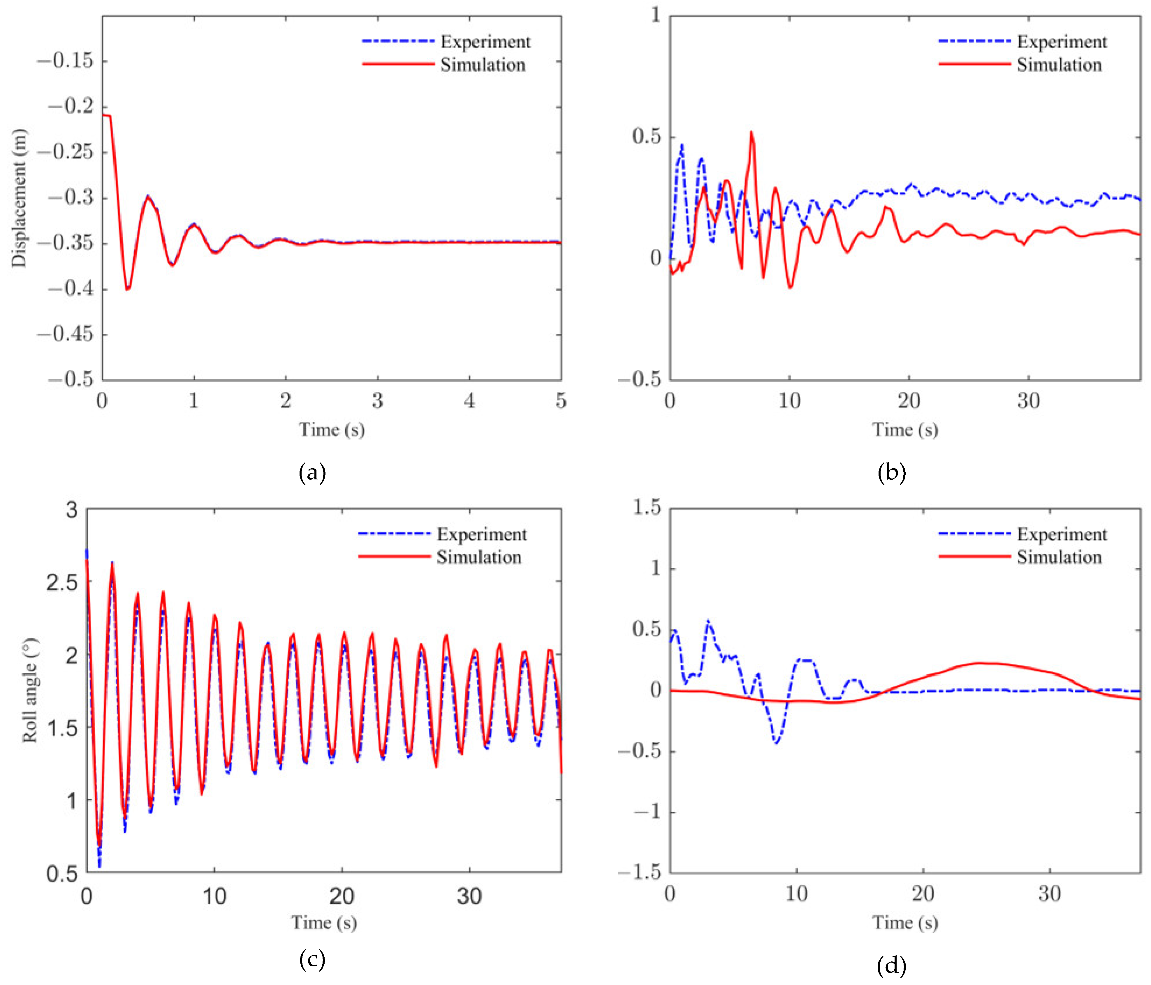
4.4. Experimental Verification of Model

An experiment was used to verify the effect of the pressing component and the simulation method on the dynamics of the FPTLIR landing. The experimental frame was built as shown in Figure 16. The following parameters were used for the experiment. (1) The type of the PTL was LGJ-95/55, and the span was 10 m. It had a diameter of 16 mm, a linear density of 707 kg/km, and an elastic modulus of 105 GPa. (2) A lifting platform was installed at the left end of the frame to adjust the slope of the PTL. (3) The 3D tilt sensor (MPU6050) was used to collect the FPTLIR’s attitude information. (4) The position of FPTLIR was measured by an IMU. (5) The FSR used was the IMS003-C10A-50, which was attached to the surface of the travelling wheel to monitor changes in contact force. It was embedded beneath the wheel surface material, with a total of six units installed to ensure that contact force could still be accurately measured even in cases of slippage at the contact points. (6) The PC was used to communicate with the STM32 and FSR data acquisition card for FSR to collect experimental data. The parameters were set in MATLAB to match those used in the experiment. The simulation was run for 40 s with a convergence criterion of $1\times {10}^{-3}$. A total of 20 nodes were set up for the simulation.

The comparison between experimental and simulation results demonstrates that the simulation model exhibits strong fitting capability to the experimental data (Figure 17). For Z-displacement, the experimental initial amplitude was ±0.1 m, while the simulation result was also ±0.1 m, and both showed a damped oscillation pattern. The pitch angle had an experimental initial amplitude of ±0.5°, while the simulation was ±0.3°, with slight fluctuations persisting after stabilization. The roll angle’s initial amplitude was ±2.5° in both the experiment and simulation, but the simulation decayed more slowly, stabilizing around 15 s with a smoother trend, whereas high-frequency vibrations persisted up to 20 s in the experiment.

For the yaw angle, the experimental results oscillated near 0° before stabilizing around that value, while the simulation stabilized near 0°. The stabilization trends were similar. Regarding contact force in Figure 18, the force value rose rapidly in the initial stage, with the experiment peaking at 400 N around 5 s, stabilizing at approximately 380 N. The simulation displayed a similar trend but with smoother results. However, experimental data showed oscillations after 5 s, likely due to changes in the contact area caused by FPTLIR attitude adjustments. The comparison of experimental and simulation data through the calculation of mean relative error (MRE) is shown in

Table 3. Comparison of MRE.

Z-Displacement	Pitch	Roll	Yaw	Contact Force
0.004	2.14	0.044	21.1	0.079

.

Overall, the simulation model effectively captures the system’s dynamic trends and aligns well with experimental results. The MRE of the Z-displacement, contact force, and roll angle is relatively small, with values of 0.004, 0.044, and 0.079, respectively.

The discrepancies, primarily in amplitude and stabilization time, are likely due to external disturbances in the experimental system or simplifications in the simulation model. The relatively larger MRE in the roll angle and yaw angle was attributed to their smaller fluctuation ranges and relatively higher susceptibility to interference. Nevertheless, the simulation model reproduces the key dynamic characteristics of the contact force, Z-displacement, and angles, demonstrating a high reliability in predicting system dynamics under ideal conditions.

5. Discussion

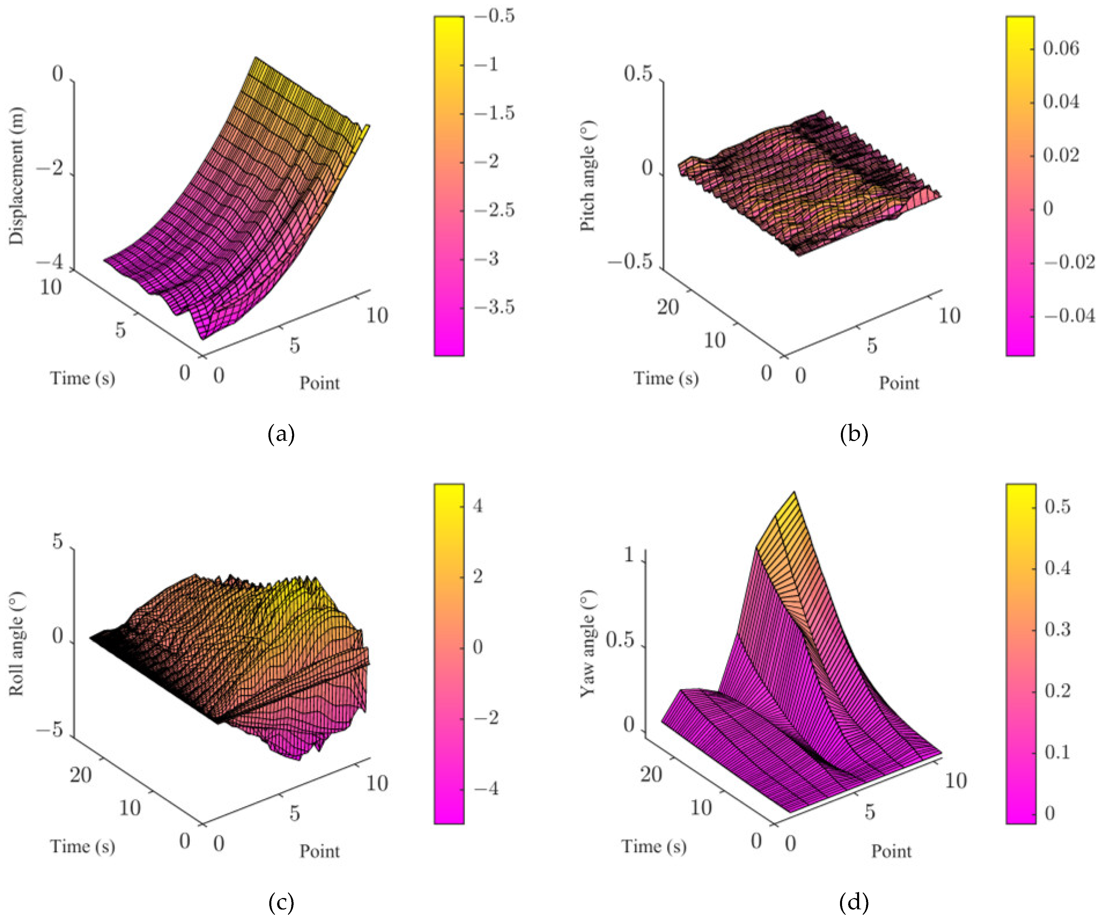
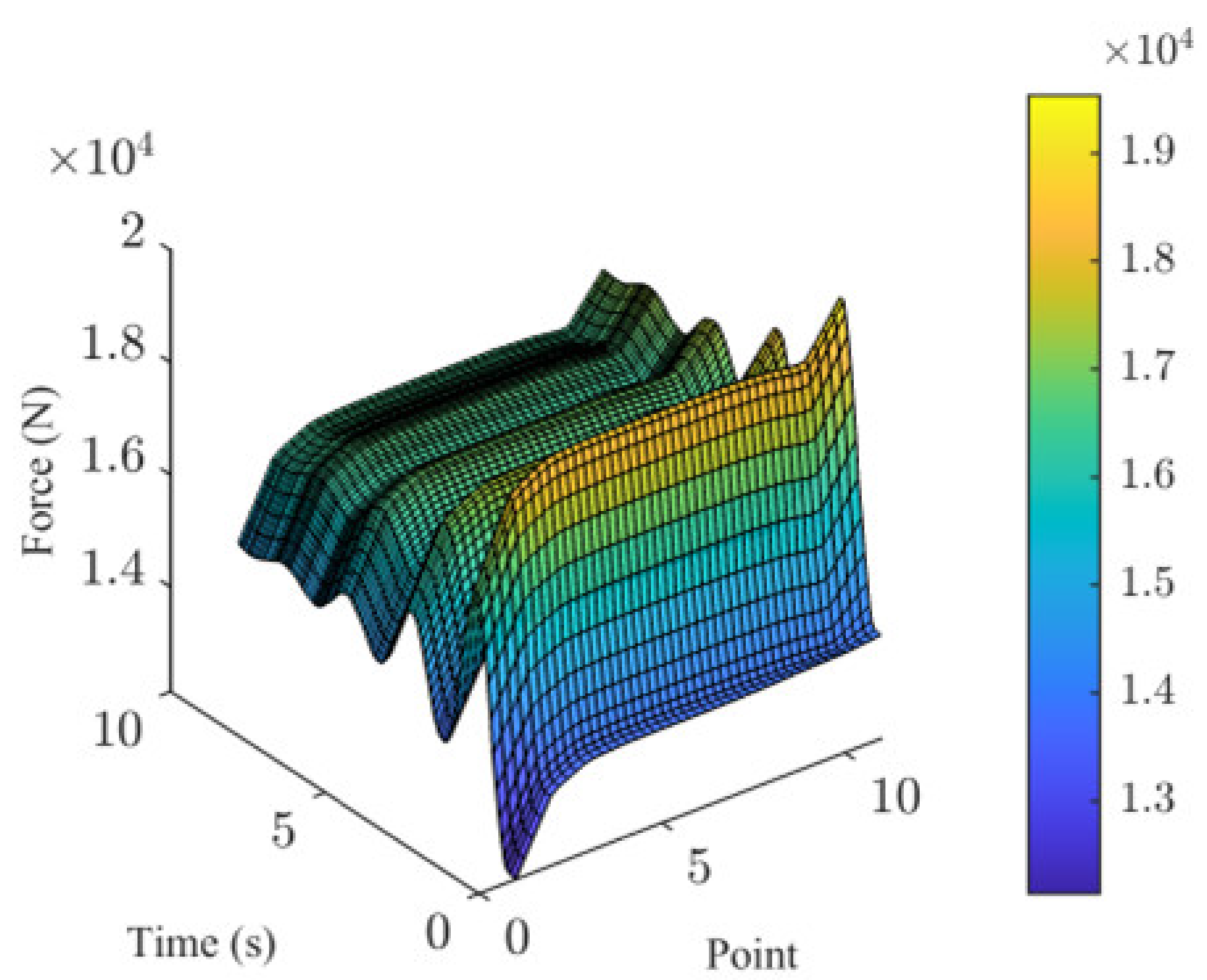
5.1. Influence of Landing Location on System Dynamics

The primary objective of the simulation experiment was to investigate the dynamic response of the FPTLIR landing points on the PTL. The simulation results were carefully analyzed to determine the initial peak values and rise times of the system’s dynamic parameters at different positions in Figure 19a. The peak Z-displacements and roll angle of the different points were all determined to be in the safe workplace.

The relative peak Z-displacement varied between −0.82 m and −0.28 m, indicating a significant influence of the landing point on this parameter. The relative peak Z-displacement showed a progressive reduction from point 1, which was far from the tower, to point 11, which was close to the tower. The peak Z-displacement at landing point 11 was found to be 34.14% of the value observed at point 1. Regarding the FPTLIR’s attitudes, the peaks showed variability in response to different landing points. Due to the smaller fluctuation amplitudes of the pitch and yaw angles compared to the roll angle, the current analysis focuses on the variation characteristics of the roll angle. Overall, the roll angle peaks increased as the FPTLIR approached the tower, ranging between 0.1° and 4.98°, with the highest peak observed at 4.98° when landing at point 9. The roll angle at landing point 9 was found to be 3.7% of the value observed at point 1.

The peak time for Z-displacement varied between 0.61 s and 2.02 s, while the roll angle’s peak time ranged from 2.43 s to 4.49 s (Figure 19b). The roll angle’s peak time consistently exceeded that of the Z-displacement, as gravity, being the sole external force, caused the FPTLIR to first reach its peak along the gravitational direction before deflecting. This trend arose from the strong coupling effect between the Z-displacement and the roll angle within the system. Despite varying landing points, the peak times remained relatively stable when the same mass was considered.

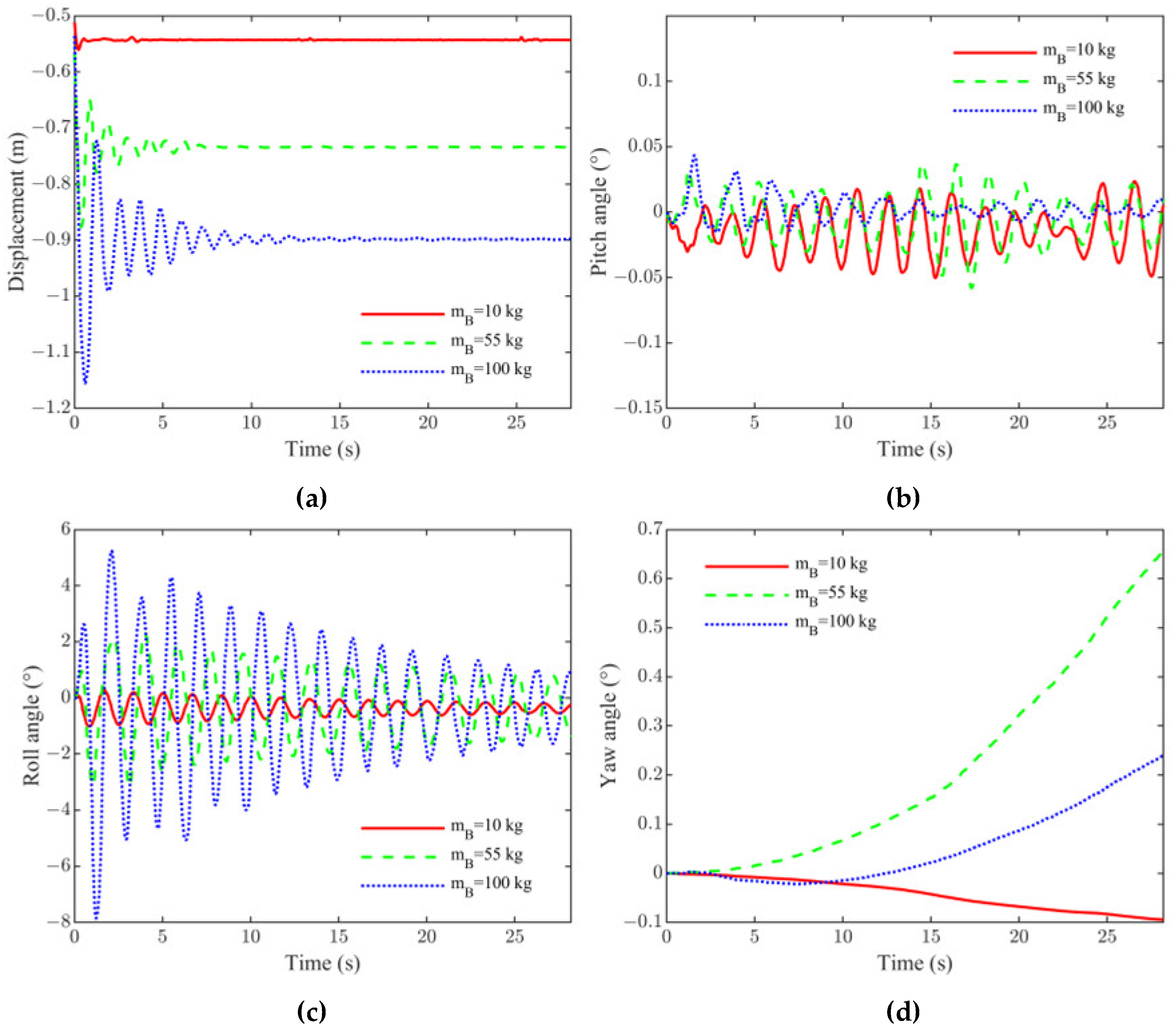
5.2. Influence of Mass of FPTLIR on System Dynamics

The aim of the simulation experiment was to study the dynamic response of FPTLIRs with different masses, ranging from 10 kg to 100 kg, when landing at the center of the PTL. The simulation results of initial peak values and rise times for FPTLIR of different masses are shown in Figure 20a. The peak Z-displacements and roll angle of different mass were also all in the safe workplace. The peak value of the Z-displacement was found to be significantly influenced by the mass of the FPTLIR. For an FPTLIR mass of 10 kg, the peak value of the relative Z-displacement was −0.06 m, while for an FPTLIR mass of 100 kg the peak value of the relative Z-displacement was −0.65 m. The peak value of the relative Z-displacement increased gradually, with the peak value for a 10 kg FPTLIR being 9.2% of a 100 kg FPTLIR. The roll angle peaks increased proportionally with the FPTLIR’s mass rising from 1.0° at 10 kg to 7.8° at 100 kg. Notably, the peak for 10 kg was only 12.8% of the peak value for 100 kg, highlighting the significant effect of increased mass on roll angle amplitude.

Figure 20b reveals that the peak time for the Z-displacement varied between 0.52 s and 0.91 s, depending on the FPTLIR’s mass, while the peak time for the roll angle ranged from 1.05 s to 1.40 s. Larger masses led to greater Z-displacement and roll angles due to higher inertia, which in turn resulted in a slower response time for the FPTLIR to reach its peak values.

5.3. Comparison Between HIRs

As shown in

Table 4. Comparison between hybrid robots.

Model	Hybrid Robot I [11]	LineDrone [12]	Hybrid Robot II [13]	FPTLIR
Hybrid layout	Bottom	Bottom	Bottom	Top
Landing	Yes	Yes	Yes	Yes
Wheel numbe	3	4	2	3
PTL model	Rigid	/	/	Flexible
Contact	Static	/	/	Dynamic

, we compared the robot’s configuration of hybrid layout (bottom indicates that the travelling mechanism is positioned below the flight mechanism), landing capability, and modeling approaches for PTL and contact forces. The advantage of the top hybrid layout is in having a more stable condition when connected to the PTL. Different from other robots, FPTLIR’s top hybrid layout maintains a stable connection to PTLs without requiring lower center of gravity positioning. We also propose a safety analysis method for the FPTLIR. Our model incorporates the flexibility of the PTL and the dynamic contact between walking wheels and the PTL, ensuring the accuracy of the dynamic landing process.

5.4. Limitations and Future Work

The limitations of the present study can be found mainly in the following two aspects:

1. In the contact force model, the contact length $l_0$ between the travelling wheel and the PTL may vary with the contact force. If the stiffness of the PTL is low, this should be considered as a variable in the model.

2. In the cable model, the more beam elements that make up the PTL, the more accurate the results, but the longer the calculation time. In this study, beam elements of equal length were used to describe the PTL. Alternatively, elements of unequal length could be used to describe the PTL, ensuring accuracy without increasing the computation time.

Although the FPTLIR/PTL dynamic model has been established, future studies should refine the model to enhance its accuracy and computational efficiency, incorporate wind disturbance effects, and investigate control strategies for FPTLIR landing positions based on its dynamic response characteristics, such as implementing roll compensation for the farthest landing points.

6. Conclusions

This study has established a coupled dynamic model of the FPTLIR and PTL. By employing the ANCF, the nonlinear large deformation and large rotation behaviors of the PTL were accurately modeled. The Hunt–Crossley contact model was adopted to simulate the dynamic interaction between the FPTLIR and the flexible PTL during landing, effectively resolving the limitations of traditional approaches that oversimplify contact force dimensions and neglect groove angle effects. Experimental and simulation results validated the accuracy of the proposed dynamic model, establishing a robust foundation for future dynamic analyses and providing theoretical insights to ensure safe FPTLIR landing in complex environments. The main conclusions are given as follows:

• A coupled FPTLIR/PTL dynamic model was derived using the ANCF method. Shear and torsion were ignored using a Euler–Bernoulli beam to improve the efficiency. The coupled effect between the FPTLIR and PTL was formulated using the Hunt–Crossley contact model, considering the deflection angle and the groove of the of the travelling wheel to ensure the accuracy.
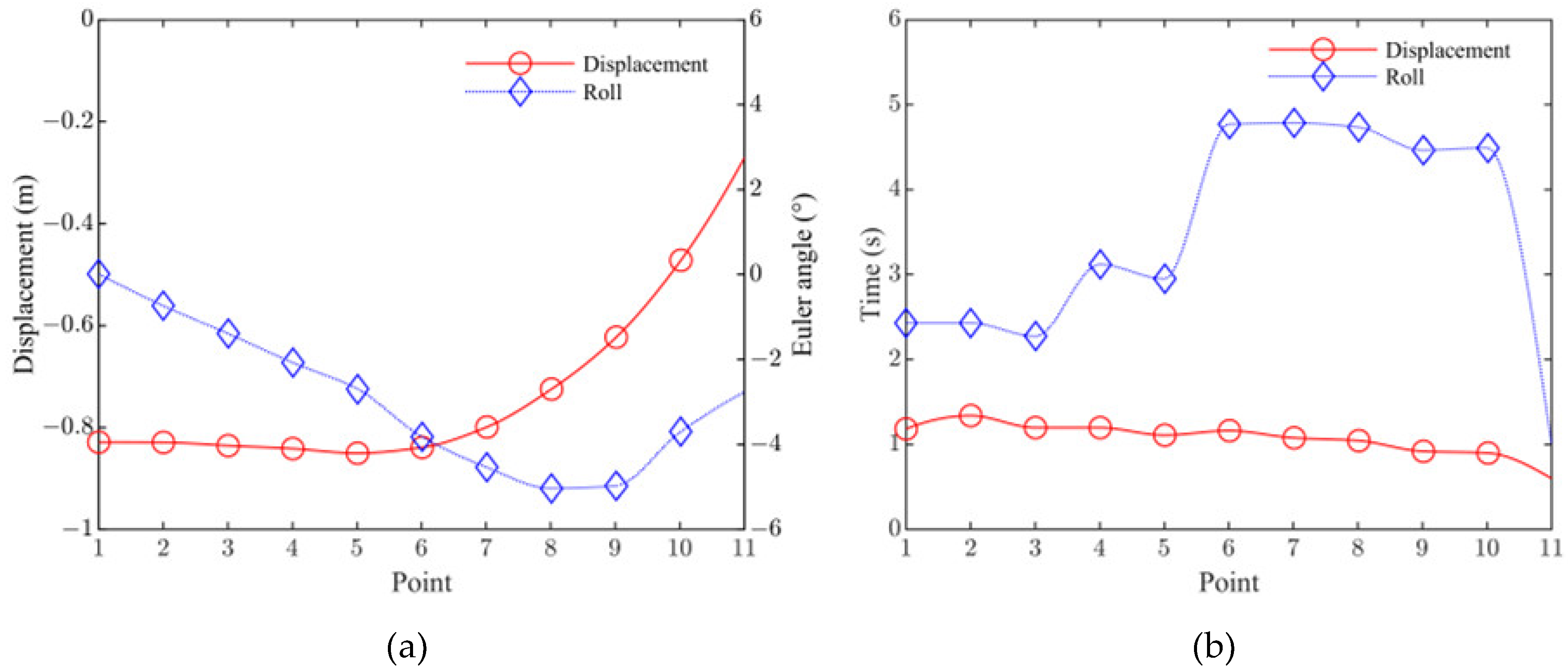
• A modular simulation of the model was performed with different landing positions and FPTLIR masses. Compared with the FEM, the ANCF demonstrated an accuracy improvement exceeding 50%. The results show that all dynamic responses remained within acceptable ranges. As the landing position approached the tower, the amplitude of the Z-displacement wave decreased, with the peak Z-displacement at the closest point being 34.4% of that at the farthest point while the roll angle amplitude increased, with the maximum exceeding the minimum by 3.7%. The appropriate landing point should be selected by weighing the collision risk against the insulation risk. Additionally, increasing the FPTLIR mass amplified the Z-displacement and attitude angle waves, with the lightest robot achieving a Z-displacement peak 9.2% and a roll angle peak 12.8% of those of the heaviest. Therefore, both the collision risk and the insulation risk exhibited a positive correlation with the robot’s mass.
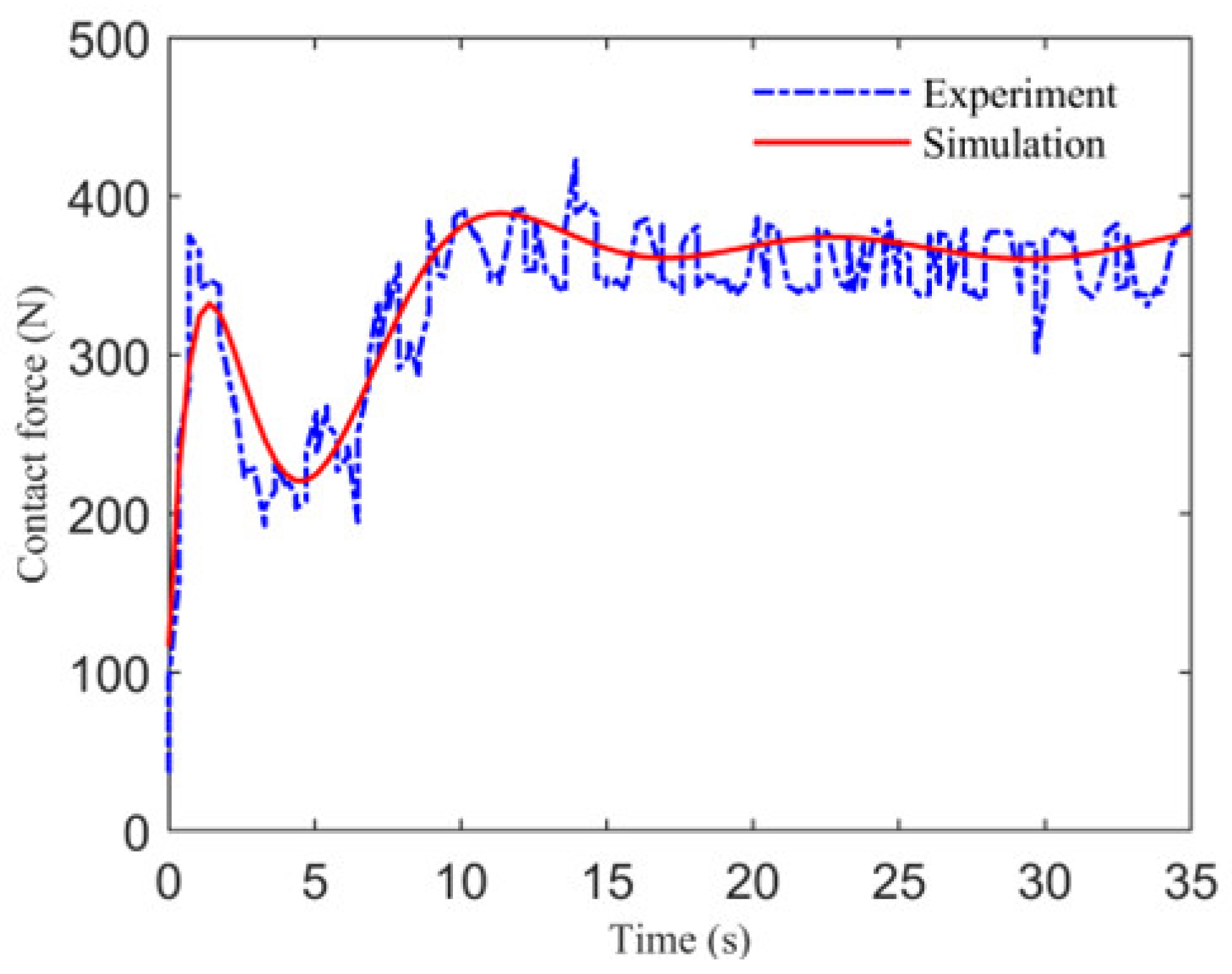
• An integrated landing test platform was constructed to observe the landing process of the FPTLIR and to validate the accuracy of the model. The time domain variations of the attitude, Z-displacements, and contact forces were measured from the test platform, with the contact forces recorded using six opposing FSRs. The results show that the relative errors for the roll angle and Z-displacement were found to be 0.004 and 0.044, respectively, validating the accuracy of the proposed method. The platform enabled accurate analysis and prediction of FPTLIR system responses during the landing process.

This study provides a methodological framework applicable not only to HIRs, but also to other robotic systems in rigid–flexible coupling environments, such as space-deployable robots, surgical robots, soft continuum robots, and cable-driven inspection robots.

References

1. Shu, Y.; Chen, W. Research and Application of UHV Power Transmission in China. High Volt. 2018, 3, 1–13. [Google Scholar] [CrossRef]
2. Yang, L.; Fan, J.; Liu, Y.; Li, E.; Peng, J.; Liang, Z. A Review on State-of-the-Art Power Line Inspection Techniques. IEEE Trans. Instrum. Meas. 2020, 69, 9350–9365. [Google Scholar] [CrossRef]
3. Ahmed, M.F.; Mohanta, J.C.; Sanyal, A. Inspection and Identification of Transmission Line Insulator Breakdown Based on Deep Learning Using Aerial Images. Electr. Power Syst. Res. 2022, 211, 108199. [Google Scholar] [CrossRef]
4. Daisy, M.; Dashti, R.; Shaker, H.R.; Javadi, S.; Hosseini Aliabadi, M. Fault Location in Power Grids Using Substation Voltage Magnitude Differences: A Comprehensive Technique for Transmission Lines, Distribution Networks, and AC/DC Microgrids. Measurement 2023, 220, 113403. [Google Scholar] [CrossRef]
5. Chen, D.; Guo, X.; Huang, P.; Li, F. Safety Distance Analysis of 500 kV Transmission Line Tower UAV Patrol Inspection. IEEE Lett. Electromagn. Compat. Pract. Appl. 2020, 2, 124–128. [Google Scholar] [CrossRef]
6. Alhassan, A.B.; Zhang, X.; Shen, H.; Xu, H. Power Transmission Line Inspection Robots: A Review, Trends and Challenges for Future Research. Int. J. Electr. Power Energy Syst. 2020, 118, 105862. [Google Scholar] [CrossRef]
7. Qiu, R.; Miao, X.; Zhuang, S.; Jiang, H.; Chen, J. Design and Implementation of an Autonomous Landing Control System of Unmanned Aerial Vehicle for Power Line Inspection. In Proceedings of the 2017 Chinese Automation Congress (CAC), Jinan, China, 20–22 October 2017; IEEE: Piscataway, NJ, USA, 2017; pp. 7428–7431. [Google Scholar]
8. Li, Z.; Zhang, Y.; Wu, H.; Suzuki, S.; Namiki, A.; Wang, W. Design and Application of a UAV Autonomous Inspection System for High-Voltage Power Transmission Lines. Remote Sens. 2023, 15, 865. [Google Scholar] [CrossRef]
9. Chen, M.; Cao, Y.; Tian, Y.; Li, E.; Liang, Z.; Tan, M. A Passive Compliance Obstacle-Crossing Robot for Power Line Inspection and Maintenance. IEEE Rob. Autom. Lett. 2023, 8, 2772–2779. [Google Scholar] [CrossRef]
10. Chang, W.; Yang, G.; Yu, J.; Liang, Z.; Cheng, L.; Zhou, C. Development of a Power Line Inspection Robot with Hybrid Operation Modes. In Proceedings of the 2017 IEEE/RSJ International Conference on Intelligent Robots and Systems (IROS), Vancouver, BC, Canada, 24–28 September 2017; IEEE: Piscataway, NJ, USA, 2017; pp. 973–978. [Google Scholar]
11. Wang, H.; Li, E.; Yang, G.; Guo, R. Design of an Inspection Robot System with Hybrid Operation Modes for Power Transmission Lines. In Proceedings of the 2019 IEEE International Conference on Mechatronics and Automation (ICMA), Tianjin, China, 4–7 August 2019; IEEE: Piscataway, NJ, USA, 2019; pp. 2571–2576. [Google Scholar]
12. Mirallès, F.; Hamelin, P.; Lambert, G.; Lavoie, S.; Pouliot, N.; Montfrond, M.; Montambault, S. LineDrone Technology: Landing an Unmanned Aerial Vehicle on a Power Line. In Proceedings of the 2018 IEEE International Conference on Robotics and Automation (ICRA), Brisbane, QLD, Australia, 21–25 May 2018; IEEE: Piscataway, NJ, USA, 2018; pp. 6545–6552. [Google Scholar]
13. Li, Z.; Tian, Y.; Yang, G.; Li, E.; Zhang, Y.; Chen, M.; Liang, Z.; Tan, M. Vision-Based Autonomous Landing of a Hybrid Robot on a Powerline. IEEE Trans. Instrum. Meas. 2023, 72, 1–11. [Google Scholar] [CrossRef]
14. Hamelin, P.; Miralles, F.; Lambert, G.; Lavoie, S.; Pouliot, N.; Montfrond, M.; Montambault, S. Discrete-Time Control of LineDrone: An Assisted Tracking and Landing UAV for Live Power Line Inspection and Maintenance. In Proceedings of the 2019 International Conference on Unmanned Aircraft Systems (ICUAS), Atlanta, GA, USA, 11–14 June 2019; IEEE: Piscataway, NJ, USA, 2019; pp. 292–298. [Google Scholar]
15. Li, Z.; Tian, Y.; Yang, G.; Zhang, Y.; Li, E.; Liang, Z.; Tan, M. Model-Based Trajectory Planning of a Hybrid Robot for Powerline Inspection. IEEE Rob. Autom. Lett. 2024, 9, 3443–3450. [Google Scholar] [CrossRef]
16. Lopes, V.M.L.; Honório, L.M.; Santos, M.F.; Pancoti, A.A.N.; Silva, M.F.; Diniz, L.F.; Mercorelli, P. Design of an Over-Actuated Hexacopter Tilt-Rotor for Landing and Coupling in Power Transmission Lines. Drones 2023, 7, 341. [Google Scholar] [CrossRef]
17. Lv, N.; Liu, J.; Xia, H.; Ma, J.; Yang, X. A Review of Techniques for Modeling Flexible Cables. Comput. -Aided Des. 2020, 122, 102826. [Google Scholar] [CrossRef]
18. Lv, N.; Liu, J.; Ding, X.; Liu, J.; Lin, H.; Ma, J. Physically Based Real-Time Interactive Assembly Simulation of Cable Harness. J. Manuf. Syst. 2017, 43, 385–399. [Google Scholar] [CrossRef]
19. Zhang, H.; Guo, J.; Liu, J.; Ren, G. An Efficient Multibody Dynamic Model of Arresting Cable Systems Based on ALE Formulation. Mech. Mach. Theory 2020, 151, 103892. [Google Scholar] [CrossRef]
20. Xiao, X.; Wu, G.; Li, S. Dynamic Coupling Simulation of a Power Transmission Line Inspection Robot with Its Flexible Moving Path When Overcoming Obstacles. In Proceedings of the 2007 IEEE International Conference on Automation Science and Engineering, Scottsdale, AZ, USA, 22–25 September 2007; IEEE: Piscataway, NJ, USA, 2007; pp. 326–331. [Google Scholar]
21. Deng, X.; Deng, Z.; Ren, X. New Algorithm of Shape-Finding of Suspension Bridge with Spatial Cables. Theor. Appl. Mech. Lett. 2023, 13, 100402. [Google Scholar] [CrossRef]
22. Fan, W.; Ren, H.; Zhu, W.; Zhu, H. Dynamic Analysis of Power Transmission Lines With Ice-Shedding Using an Efficient Absolute Nodal Coordinate Beam Formulation. J. Comput. Nonlin. Dyn. 2021, 16, 011005. [Google Scholar] [CrossRef]
23. Gu, Y.; Lan, P.; Cui, Y.; Li, K.; Yu, Z. Dynamic Interaction between the Transmission Wire and Cross-Frame. Mech. Mach. Theory 2021, 155, 104068. [Google Scholar] [CrossRef]
24. Peng, C.; Yang, C.; Xue, J.; Gong, Y.; Zhang, W. An Adaptive Variable-Length Cable Element Method for Form-Finding Analysis of Railway Catenaries in an Absolute Nodal Coordinate Formulation. Eur. J. Mech. -A/Solids 2022, 93, 104545. [Google Scholar] [CrossRef]
25. Zheng, X.; Wu, G.; Jiang, W.; Fan, F.; Zhu, J. Rigid–Flexible Coupling Dynamics with Contact Estimator for Robot/PTL System. Proc. Inst. Mech. Eng. K J. Multi-Body Dyn. 2020, 234, 635–649. [Google Scholar] [CrossRef]
26. Xiao, X.; Wu, G.; Du, E.; Li, S. Impacts of Flexible Obstructive Working Environment on Dynamic Performances of Inspection Robot for Power Transmission Line. J. Cent. South Univ. Technol. 2008, 15, 869–876. [Google Scholar] [CrossRef]
27. Yue, X.; Wang, H.; Jiang, Y. Performance Optimization of a Mobile Inspection Robot for Power Transmission Lines. Int. J. Simul. Syst. Sci. Technol. 2016, 17, 3.1–3.3. Available online: https://ijssst.info/Vol-17/No-48/paper3.pdf (accessed on 7 February 2025).
28. Westin, C.; Irani, R.A. Modeling Dynamic Cable–Sheave Contact and Detachment during Towing Operations. Mar. Struct. 2021, 77, 102960. [Google Scholar] [CrossRef]
29. Wang, Y.; Qin, X.; Jia, W.; Lei, J.; Wang, D.; Feng, T.; Zeng, Y.; Song, J. Multiobjective Energy Consumption Optimization of a Flying–Walking Power Transmission Line Inspection Robot during Flight Missions Using Improved NSGA-II. Appl. Sci. 2024, 14, 1637. [Google Scholar] [CrossRef]
30. Bauchau, O.A.; Craig, J.I. Euler-Bernoulli Beam Theory. In Structural Analysis; Bauchau, O.A., Craig, J.I., Eds.; Springer: Dordrecht, The Netherlands, 2009; pp. 173–221. ISBN 978-90-481-2516-6. [Google Scholar]
31. Gerstmayr, J.; Irschik, H. On the Correct Representation of Bending and Axial Deformation in the Absolute Nodal Coordinate Formulation with an Elastic Line Approach. J. Sound Vib. 2008, 318, 461–487. [Google Scholar] [CrossRef]
32. Atay, S.; Buckner, G.; Bryant, M. Dynamic Modeling for Bi-Modal, Rotary Wing, Rolling-Flying Vehicles. J. Dyn. Syst. Meas. Contr. 2020, 142, 111003. [Google Scholar] [CrossRef]
33. Zengin, A.T.; Erdemir, G.; Akinci, T.C.; Selcuk, F.A.; Erduran, M.N.; Seker, S.S. (PREPRINT) ROSETLineBot: One-Wheel-Drive Low-Cost Power Line Inspection Robot Design and Control. J. Electr. Syst. 2019, 15, 626–634. [Google Scholar]
34. Pouliot, N.; Montambault, S. Geometric Design of the LineScout, a Teleoperated Robot for Power Line Inspection and Maintenance. In Proceedings of the 2008 IEEE International Conference on Robotics and Automation, Pasadena, CA, USA, 19–23 May 2008; IEEE: Piscataway, NJ, USA, 2008; pp. 3970–3977. [Google Scholar]
Figure 1. Schematic diagram of the FPTLIR working in an overhead PTL environment.
Applsci 15 01863 g001
Figure 2. Analysis framework for the research.
Applsci 15 01863 g002
Figure 3. Schematic diagram of the operating zones of attitude for the FPTLIR: (a) roll workspace; (b) yaw workspace; (c) pitch workspace; (d) zoomed-in view of yaw workplace.
Applsci 15 01863 g003
Figure 4. Line shape and slope changes of a 200 m PTL: (a) PTL shape; (b) PTL slope.
Applsci 15 01863 g004
Figure 5. Schematic diagram of the operating zones in the Z direction for the FPTLIR.
Applsci 15 01863 g005
Figure 6. The FPTLIR lands on a segment of the PTL and the k t h 12-degree element.
Applsci 15 01863 g006
Figure 7. The contact cross-section between the travelling wheel and the PTL.
Applsci 15 01863 g007
Figure 8. The workflow of modular simulation.
Applsci 15 01863 g008
Figure 9. Simulation diagram of the FPTLIR in the ADAMS software.
Applsci 15 01863 g009
Figure 10. ADAMS simulation workflow.
Applsci 15 01863 g010
Figure 11. Dynamic behavior error of the FPTLIR: (a) displacement error; (b) roll error.
Applsci 15 01863 g011
Figure 12. Time history of the attitude and Z-displacement of the FPTLIR.
Applsci 15 01863 g012
Figure 13. FPTLIR Z-displacement and attitude at different landing points: (a) Z-displacement; (b) pitch angle; (c) roll angle; (d) yaw angle.
Applsci 15 01863 g013
Figure 14. Tension variation in the PTL at different locations when the FPTLIR lands at the midpoint.
Applsci 15 01863 g014
Figure 15. The Z-displacement t and attitude changes of FPTLIRs with different masses during landing at the midpoint of the PTL: (a) Z-displacement; (b) pitch angle; (c) roll angle; (d) yaw angle.
Applsci 15 01863 g015
Figure 16. Experiment of the FPTLIR walking along the PTL.
Applsci 15 01863 g016
Figure 17. Comparison of dynamic responses between experiment and simulation: (a) Z-displacement; (b) pitch angle; (c) roll angle; (d) yaw angle.
Applsci 15 01863 g017
Figure 18. Comparison of contact forces between experiment and simulation.
Applsci 15 01863 g018
Figure 19. Comparison of the peak values and rise times of FPTLIR Z-displacement and roll angle at different landing points on the PTL: (a) peak value; (b) rise time.
Applsci 15 01863 g019
Figure 20. A comparison of the peak values and rise times for FPTLIR Z-displacement and roll angle when FPTLIRs with different masses land at the midpoint of the PTL: (a) peak values; (b) rise time.
Applsci 15 01863 g020